THREE ANCIENT HALO SUBGIANTS: PRECISE PARALLAXES, COMPOSITIONS, AGES, AND IMPLICATIONS FOR GLOBULAR CLUSTERS

Abstract

The most accurate ages for the oldest stars are those obtained for nearby halo subgiants, because they depend almost entirely on just the measured parallaxes and absolute oxygen abundances. In this study, we have used the Fine Guidance Sensors on the Hubble Space Telescope to determine trigonometric parallaxes, with precisions of 2.1% or better, for the Population II subgiants HD 84937, HD 132475, and HD 140283. High quality spectra have been used to derive their surface abundances of O, Fe, Mg, Si, and Ca, which are assumed to be 0.1–0.15 dex less than their initial abundances due to the effects of diffusion. Comparisons of isochrones with the three subgiants on the $(\log{T_{\rm eff}},\,M_{V})$-diagram yielded ages of $12.08\pm 0.14$, $12.56\pm 0.46$, and $14.27\pm 0.38$ Gyr for HD 84937, HD 132475, and HD 140283, in turn, where each error bar includes only the parallax uncertainty. The total uncertainty is estimated to be $\sim\pm 0.8$ Gyr (larger in the case of the near-turnoff star HD 84937). Although the age of HD 140283 is greater than the age of the universe as inferred from the cosmic microwave background by $\sim 0.4$–0.5 Gyr, this discrepancy is at a level of $<1\,\sigma$. Nevertheless, the first Population II stars apparently formed very soon after the Big Bang. (Stellar models that neglect diffusive processes seem to be ruled out as they would predict that HD 140283 is $\sim 1.5$ Gyr older than the universe.) The field halo subgiants appear to be older than globular clusters of similar metallicities: if distances close to those implied by the RR Lyrae standard candle are assumed, M 92 and M 5 are younger than HD 140283 and HD 132475 by $\sim 1.5$ and $\sim 1.0$ Gyr, respectively.

1 Introduction

Stars with extremely low metal abundances are of particular astrophysical and cosmological interest because they probe very early times in the evolution of the universe and its galactic components. However, it is very difficult to determine their absolute ages to within $\sim 15$–20%. Nearly all of the metal-poor stars that can be age-dated reliably are found in globular clusters (GCs) or dwarf galaxies, but even when tight, well-defined color-magnitude diagrams (CMDs) are available for them, the ages that are inferred from fits of isochrones to the observed CMDs depend critically on the adopted distances and chemical abundances. For instance, a $\pm 0.10$ mag uncertainty in the assumed distance modulus translates to a change in the estimated age by $\sim\,\mathrel{\hbox{\raise 3.01385pt\hbox{$-$}\kern-7.3194pt\lower 0.43057pt\hbox{$+$}}}1$ Gyr — which is also implied by the assumption of an oxygen abundance that is altered by $\delta(\log\,N)\approx\pm 0.3$ (see, e.g., VandenBerg et al. 2012). In view of such sensitivities, it is not surprising that recent estimates of the ages of well-studied GCs like M 92 (e.g., di Cecco et al. 2010, VandenBerg et al. 2013) and 47 Tucanae (e.g., Dotter et al. 2010, Hansen et al. 2013) range over as much as 2–3 Gyr.

Ages of considerably higher accuracy are possible for field Population II stars if they are close enough that accurate and precise trigonometric parallaxes can be obtained for them and they are in the subgiant phase of evolution. Isochrones for different ages are most widely separated in the region of a CMD between the turnoff (TO) and the base of the red-giant branch (RGB); i.e., the luminosities of stars, at a fixed effective temperature (${T_{\rm eff}}$) or color, are predicted to depend most strongly on age when they are evolving along what is usually referred to as the subgiant branch (SGB). As a consequence, the ages of such stars can be determined directly from their locations relative to isochrones that have been computed for their observed chemical abundances. Although the ramifications of temperature and/or color uncertainties are not insignificant, such comparisons between theory and observations benefit from the fact that the slope of the SGB is relatively shallow on the $(\log{T_{\rm eff}},\,\log\,L)$-diagram and most CMDs. A further big advantage of studying nearby SGB stars, as opposed to their counterparts in considerably more distant systems, is that much higher resolution, higher S/N spectra may be used to determine their metal abundances. Moreover, the foreground reddenings are small and they can be determined precisely from the interstellar Na i D lines.

HD 140283, which has long been known to have [Fe/H] $\sim-2.4$ (e.g., Nissen et al. 2004, Bessell 2007, Casagrande et al. 2010), is the most famous example of a solar-neighborhood subgiant that provides a direct constraint on the ages of field stars of similar metallicity due to its auspicious location on the H-R diagram. The parallax that was initially derived for it, $\pi=17.44\pm 0.97$ mas, from measurements taken with the Hipparcos astrometric satellite (Perryman et al. 1997) yielded $M_{V}\approx 3.30\pm 0.12$, depending on the adopted apparent magnitude, reddening, and the statistical corrections that were applied (e.g., Pont et al. 1998, Carretta et al. 2000). The corresponding age of HD 140283 was determined to be $13.5\pm 1.4$ Gyr (where the error bar takes into account only the distance uncertainty) by VandenBerg et al. (2002), using isochrones based on University of Montreal stellar models that treated all of the important diffusive processes (Richard et al. 2002). At nearly the same time, the age of the universe was found to be $13.7\pm 0.2$ Gyr from the analysis by Spergel et al. (2003) of first-year Wilkinson Microwave Anisotropy Probe (WMAP) observations of the cosmic microwave background (CMB). The similarity of these results suggests that HD 140283 has the potential to provide an interesting test of stellar physics and cosmology, and to contribute to our understanding of the first epochs of star formation in the early universe, if its age can be pinned down much more precisely.

To this end, we began a program in 2003 August to improve upon the Hipparcos parallaxes of HD 140283 and the two other nearest metal-deficient subgiants, HD 84937 and HD 132475, using the Fine Guidance Sensors (FGSs) on the Hubble Space Telescope (HST). [HD 140283 and HD 132475, which differ in [Fe/H] by $\sim 1$ dex, are arguably the best candidates for such a study because they are located approximately midway between the TO and the lower RGB; see VandenBerg (2000, his Figs. 9 and 32). HD 84937 lies closer to the TO, and in fact, it has sometimes been considered to be a blue straggler; e.g., Bond & MacConnell (1971).] As reported by Bond et al. (2013), our reduction of the observations of HD 140283 that were obtained between 2003 and 2011 resulted in a value of $\pi=17.15\pm 0.14$ mas, which agrees remarkably well with the value derived by van Leeuwen (2007, $\pi=17.16\pm 0.68$ mas) in his re-analysis of the original Hipparcos data, but with a factor of 5 improvement in the precision of the result. On the assumption of $V=7.205\pm 0.02$ (Casagrande et al. 2010) and $E(B-V)=0.000\pm 0.002$ (Meléndez et al. 2010), the FGS parallax yielded an absolute magnitude $M_{V}=3.377\pm 0.027$. According to the many published spectroscopic studies that were consulted (see the Bond et al. paper for references), HD 140283 has [Fe/H] $=-2.4\pm 0.10$ and [O/H] $=-1.67\pm 0.15$: these values were adjusted by $+0.1$ and $+0.13$ dex, respectively, to compensate for the predicted effects of diffusion and turbulent mixing on its surface abundances over its lifetime (Richard et al. 2002). From up-to-date isochrones for the resultant initial metal abundances, the age of HD 140283 was found to be $14.46\pm 0.8$ Gyr, where the [O/H] and ${T_{\rm eff}}$ uncertainties contribute more to the total error bar than the distance uncertainty (which amounts to $\pm 0.31$ Gyr).

The current best estimate of the age of the universe is $13.82\pm 0.06$ Gyr, based on observations of the CMB using the Planck satellite (Ade et al. 2013), in excellent agreement with the latest WMAP derivation of $13.77\pm 0.06$ Gyr (Bennett et al. 2013). Recent simulations (e.g., Ritter et al. 2012; Safranek-Shrader, Milosavljević, & Bromm 2014) suggest that the oldest Population II stars probably formed $\sim 0.2$–0.3 Gyr after the Big Bang, depending on how quickly the gas from the first (Population III) supernovae was able to cool and condense, as well as such factors as the severity of the Pop. III feedback. Hence, the age that Bond et al. (2013) obtained for HD 140283 is about 0.8 Gyr older than its expected maximum age. Although 13.5–13.6 Gyr is only just outside the $1\,\sigma$ error bar on the age of HD 140283 (when all sources of error are considered), which is not a severe inconsistency, it is clearly worthwhile to take a second, hard look at all of the factors that play a role in the age determination, including the parallax, the adopted metal abundances, and the stellar models. In particular, we decided to carry out our own analysis of high-resolution spectra of HD 140283 (and the other subgiants in our sample) rather than rely on published (sometimes discordant) chemical abundance determinations.

The next section provides an overview of the procedures used to derive trigonometric parallaxes using the FGSs and the results that we obtained for our target stars. Our spectroscopic analyses, the stellar models that have been used, and the determination of the ages of the subgiants are fully described in sections 3, 4, and 5, respectively. The implications of our findings for the distances, ages, and [Fe/H] scales of globular clusters is the subject of § 6, which also includes some discussion concerning the RR Lyrae $M_{V}$ versus [Fe/H] relationship. The main conclusions of this study are summarized in § 7.

2 Hubble Space Telescope FGS Astrometry

2.1 Observations and Data Analysis

Our astrometric measurements were made with the FGSs onboard the HST. They are a set of three interferometers that can sequentially measure precise positions of a target star and several surrounding astrometric reference stars with one FGS (FGS1r), while the other two (FGS2 and FGS3) are locked on guide stars in order to maintain telescope pointing. Our FGS observations of each halo subgiant consisted of two HST orbits each at five epochs, taken near the biannual dates of maximum parallax factor, for a total of 10 HST orbits per target (11 for HD 140283). The observations were made as follows: HD 84937 between 2003 November and 2005 November; HD 132475 between 2003 August and 2006 February; and HD 140283 between 2003 August and 2006 March, with an additional single orbit of observation in 2011 March.

During each HST orbit, we used FGS1r in “Position” mode to measure the relative positions of the subgiant and six or seven faint neighboring background reference stars. Each reference star was observed for about 30 s, three to four times per orbit, interspersed with five or more measurements of the subgiant. The data gathered over the course of an orbit were processed and calibrated as a single “plate.” (The repeated exposures of the same stars are used to model and remove telescope pointing drift resulting from the changing thermal environment as the HST orbits the Earth.) Guide-star telemetry from the two guiding FGSs was used to remove high-frequency spacecraft pointing jitter from the FGS1r astrometric data. Because of refractive components in the FGS optical chain, color-dependent corrections to the astrometry were applied as functions of $B-V$ color for each star (see Nelan & Bond 2013, their § 3.3 for details). Finally, the FGS data were corrected for differential velocity aberration and geometric distortion (“optical field angle distortion”) to produce the astrometric measurements from each HST orbit.

Data from the ten or eleven orbits were combined using an updated version of the least-squares overlapping-plate GAUSSFIT program (Jeffreys, Fitzpatrick, & McArthur 1988), which solves for the plate constants (rotation, translation, and scale) along with the parallax and proper motion (PM) of each star. However, since the FGS measures only relative positions, the PMs and estimated parallaxes of the reference stars must be input as priors to the model in order to obtain an absolute parallax and PM of the subgiant. We estimated the input reference-star parallaxes based on ground-based photometry and spectroscopic observations (see next subsection). Their input PMs were obtained from the PPMXL (Roeser, Demleitner, & Shilbach 2010) or UCAC4 (Zacharias et al. 2013) catalogs; we chose the input catalog for each field that yielded the lower $\chi^{2}$ value, which proved to be PPMXL for the HD 84937 field and UCAC4 for the other two. These reference-star data are provided to the model as observations with errors, not as fixed values. This allows GAUSSFIT freedom to adjust the values within their stated errors to find the overall best $\chi^{2}$ solution. We assumed a 20% uncertainty in the distance of each reference star, corresponding to a $\pm 0.4$ mag uncertainty in their absolute magnitudes. (An overview of parallax measurements with the FGSs can be found in Nelan & Makidon 2002.)

The input ground-based PMs generally have large uncertainties, relative to the high precision of the HST measurements. This results in elevated residuals in all of the other quantities computed by the model. To mitigate this, we first executed the model with the ground-based measurements and errors, and then used the resulting FGS PMs and errors as input to the next iteration. We found that, while this does not appreciably change the PMs after the first iteration, the resulting $\chi^{2}$ and residuals are generally reduced by a few tens of percent.

The $V=7.2$ brightness of HD 140283 necessitated the use of the F5ND attenuator (required for targets brighter than $V=8$) on the subgiant, while the fainter reference stars were observed using the F583W spectral element. This introduces a cross-filter wedge effect that shifts the position of HD 140283 relative to the field stars in a manner similar to parallax. Fortunately, this cross-filter shift (on the order of 8 mas) is well calibrated near the two locations in the FGS1r field of view where HD 140283 was observed over the course of the program. Nonetheless, there remains a $\sim 0.2$ mas systematic uncertainty in the cross-filter calibration, which must be added in quadrature to the statistical errors computed by GAUSSFIT. This had not been included in the uncertainties reported for HD 140283 by Bond et al. (2013), but is incorporated now. For the other two targets, HD 84937 and HD 132475, the F5ND filter was not used for any of the observations.

2.2 Reference-Star Distance Estimation

We made distance estimates for the reference stars based on ground-based spectroscopy and photometry. For spectral classification, digital spectra in all three fields were obtained by us with the WIYN 3.5-m telescope and Hydra spectrograph at Kitt Peak National Observatory (KPNO) in 2004 and 2007, and by service observers on the 1.5-m SMARTS telescope and Ritchey-Chretien spectrograph at Cerro Tololo Interamerican Observatory (CTIO) in 2003 through 2005. The classifications were then determined through comparisons with a network of MK standards obtained with the same telescopes, assisted by equivalent-width measurements of lines sensitive to temperature and luminosity.

Photometry of the reference stars in the Johnson-Kron-Cousins BVI system was obtained with the SMARTS 1.3-m telescope at CTIO, using the ANDICAM CCD camera, and calibrated to the standard-star network of Landolt (1992). Each field was observed by Chilean service observers on four different photometric nights in 2003 through 2005. Additional photometry was obtained by H.E.B. with the CTIO 0.9-m telescope on one night in 2001 and with the KPNO 0.9-m telescope on two nights in 2007; and by D.H. with the KPNO 2.1-m telescope on single nights in 2003 and 2004.

Table 1 gives the designations, coordinates, photometry, and spectral types of the reference stars in columns 1 through 7. The uncertainties in the magnitudes and colors, based on the internal agreement, are typically about $\pm 0.004$ and $\pm 0.005$ mag, respectively. To estimate the reddening of the reference stars (assumed to be the same for all stars in each field, since their distances place them well beyond the dust of the Galactic disk), we compared the observed $B-V$ color of each star with the intrinsic $(B-V)_{0}$ color corresponding to its spectral type, and calculated the average $E(B-V)$ for each field. The intrinsic colors were taken from literature compilations assembled by E. Mamajek. These averages agreed very well with $E(B-V)$ values from the extinction maps of Schlafly & Finkbeiner (2011, hereafter SF11), as implemented at the NASA/IPAC website. Our adopted values of $E(B-V)$ were 0.037, 0.100, and 0.130 mag for the background fields of HD 84937, HD 132475, and HD 140283, respectively.

For the distance estimations, we used a purely empirical approach, which is based on determining the luminosity class from the spectroscopic data, and then using the dereddened photometry to estimate the absolute magnitude, $M_{V}$. For subgiants and giants, we found the absolute magnitudes by interpolation in a fiducial sequence [$M_{V}$ vs. $(V-I)_{0}$] for the old open cluster M 67 (Sandquist 2004), which we took to be representative of the faint population at high galactic latitudes ($b=+45\fdg 5,+31\fdg 9$, and $+33\fdg 6$, in turn, for HD 84937, HD 132475, and HD 140283).

For the reference stars classified as dwarfs, we followed the algorithm described in Bond et al. (2013), which in brief is based on calibrations of the visual absolute magnitude against $B-V$ and $V-I$ colors through polynomial fits to a sample of 791 single main-sequence stars with accurate BVI photometry and Hipparcos or USNO parallaxes of 40 mas or higher (provided online by I. N. Reid). This calibration includes a correction for metallicity, estimated from each star’s position in the $B-V$ vs. $V-I$ diagram. We tested our algorithm by applying it to 136 nearby stars with accurate parallaxes and a wide range of metallicities listed by Casagrande et al. (2010). We reproduced their known absolute magnitudes with an rms scatter of only 0.28 mag. At the distances of the reference stars, ranging mostly from about 500 to 1700 pc, this scatter corresponds to parallax errors of 0.08 to 0.24 mas.

The final two columns in Table 1 give the input estimated parallaxes and associated errors for the reference stars, and the final adjusted parallax that was output by the GAUSSFIT routine. In most cases, the adjustments were quite small.

2.3 Astrometric Results

Table 2 presents our final astrometric results for the three halo subgiants. Columns 2 through 4 show the Hipparcos PM components and parallaxes, and columns 5 through 7 show our FGS results. Note that we have reanalyzed the FGS data for HD 140283 that were presented by Bond et al. (2013), using the identical procedures employed for the other two targets in the present paper. Our results for this star are thus very slightly different from those published in 2013. The error bar for HD 140283 also now includes the uncertainty due to use of the neutral-density filter, as discussed above in § 2.1.

The FGS PMs agree very well with those found by Hipparcos. However, there are slight offsets in the PM zero-points for the FGS measurements compared to the absolute PMs of Hipparcos, because the FGS reference frames are based on only about half a dozen background stars chosen from the PPMXL or UCAC4 catalogs. These catalogs have errors in the absolute PMs per star of several mas yr^-1 (e.g., Zacharias et al. 2013).

Our parallaxes likewise agree extremely well with Hipparcos for two of our targets, but our statistical uncertainties are about 2.5–4 times smaller. For HD 84937, our FGS parallax measurement is smaller than that found by Hipparcos, by about 2$\sigma$ in units of the Hipparcos uncertainty. We note that offsets of a similar amount and sign between Hipparcos parallaxes and precise FGS and/or radio-interferometric parallaxes have sometimes been found by other investigators, e.g., for the Pleiades cluster (Soderblom et al. 2005; Melis et al. 2013).

3 Atmospheric Parameters and Chemical Abundances

In this section we derive atmospheric parameters and the abundances of those elements that are of particular relevance for the determination of the ages of metal-poor stars from fits of isochrones. Most important are O and Fe, but we also comment on the abundances of C and N as well as the $\alpha$-capture elements, Mg, Si, and Ca. [We include HD 19445 among the stars that are subjected to a spectroscopic analysis because it is used in § 5 to check the reliability of isochrones for [Fe/H] $\sim-2$ at $M_{V}\approx 5$ ($\sim 1$ mag below the turnoff). HD 19445 is the best available subdwarf for this purpose because of its large and well-determined parallax from Hipparcos ($\pi=24.92\pm 0.91$ mas; van Leeuwen 2007).]

The abundances were derived from equivalent widths (EWs) measured in high-resolution UVES (Dekker et al. 2000) and HARPS spectra (Mayor et al. 2003) obtained during the ESO programs that are listed in the footnote of Table 3. An exception is HD 132475 for which the EWs of the O i triplet lines were measured from ESO/CES spectra (Jonsell et al. 2005). The UVES and HARPS spectra have resolutions around $10^{5}$ and signal-to-noise (S/N) ratios ranging from 400 to 800. As the continuum in the spectra of these metal-poor stars is well defined, the high S/N makes it possible to measure equivalent widths of weak lines with very high accuracy. A comparison of EWs measured in overlapping UVES and HARPS spectral regions shows a rms dispersion of only 0.6 mÅ, suggesting that the mean EW is measured with an accuracy of $\pm 0.3$ mÅ.

Plane parallel (1D) model atmospheres interpolated to the ${T_{\rm eff}}$, $\log\,g$, and [Fe/H] values of the stars were obtained from the $\alpha$-element enhanced ([$\alpha$/Fe] $=+0.4$) MARCS grid (Gustafsson et al. 2008) and used to calculate EWs as a function of element abundance, assuming local thermodynamic equilibrium (LTE). Interpolation to an observed EW then yields the corresponding abundance. A microturbulence of 1.4 km s^-1 was adopted. This value is obtained for HD 132475 by demanding that the derived Fe abundance shows no systematic dependence on EW. For the other stars, the lines are so weak that the microturbulence parameter has no significant effect on the derived abundances.

3.1 ${T_{\rm eff}}$ and $\log\,g$

The effective temperatures given in Table 4 are based on the calibration of the infrared flux method (IRFM) by Casagrande et al. (2010) and taken from Meléndez et al. (2010), except in the case of HD 140283. For this star, we detect weak interstellar Na i D lines ($EW=23.0$ and 11.5 mÅ), which implies $E(B-V)=0.004$ according to the calibration of Alves-Brito et al. (2010). This increases the IRFM temperature of HD 140283 from ${T_{\rm eff}}=5777$ K, as reported by Meléndez et al., who assumed $E(B-V)=0.0$, to ${T_{\rm eff}}=5797$ K. The statistical errors associated with the IRFM temperatures are on the order of $\pm 60$ K according to Casagrande et al. (2010), but in addition, there could be systematic errors of the particular ${T_{\rm eff}}$-scale that is adopted. For instance, using a different implementation of the IRFM based on 2MASS photometry, González Hernández & Bonifacio (2009) derived $T_{\rm eff}$ values for HD 19445, HD 84937, and HD 140283 that are an average of 80 K cooler than those by Casagrande et al. In the case of HD 132475, they find a higher temperature (5815 K), but this is probably because they assume a reddening of $E(B-V)=0.03$ instead of the value that we favor, $E(B-V)=0.007$, which is based on the strength of interstellar Na i D lines.

As a check of the ${T_{\rm eff}}$-scale, we have compared the IRFM-based temperatures with those derived from the wings of the Balmer lines. This spectroscopic determination has the advantage of being independent of interstellar reddening. For the best studied star, HD 140283, Gehren et al. (2004) obtained ${T_{\rm eff}}=5773$ K from H$\alpha$ and H$\beta$, while Asplund et al. (2006) found ${T_{\rm eff}}=5753$ K from H$\alpha$ and Nissen et al. (2007) determined ${T_{\rm eff}}=5849$ K from H$\beta$. The average of these values, 5791 K, agrees well with our IRFM temperature of 5797 K, but as discussed by Nissen et al., there may be systematic errors in the Balmer-line temperatures related to the temperature structures of model atmospheres, non-LTE effects, and line-broadening theory. For 10 halo stars having $T_{\rm eff}$ from both H$\alpha$ and H$\beta$, the H$\beta$ temperatures are systematically higher than those from H$\alpha$ by $\Delta T_{\rm eff}=64\pm 28$ K. This suggests that the spectroscopic ${T_{\rm eff}}$-scale is uncertain by approximately $\pm 70$ K. Furthermore, for a sample of 30 metal-poor halo stars, Casagrande et al. (2010) compared their IRFM temperatures with those derived from the hydrogen lines by Bergemann (2008) and Nissen et al. (2007). As seen in their Fig. 12, there is good agreement between the two scales at $5600<{T_{\rm eff}}\ <6000$ K, whereas the IRFM temperatures tend to be higher by 50 to 100 K at ${T_{\rm eff}}>6100$ K. In summary, we conclude that there is no evidence from the presently available spectroscopic temperatures of halo stars that the Casagrande et al. (2010) IRFM scale is too low, but it may be 50–100 K too high for metal-poor halo stars in the turnoff region.

Surface gravities are derived from the standard relation

$$\log\frac{g}{g_{\odot}}=\log\frac{\cal{M}}{\cal{M}_{\odot}}+4\log\frac{T_{\rm eff}}{T_{\rm eff,\odot}}+0.4(M_{\rm bol}-M_{{\rm bol},\odot})$$ (1)

where $\cal{M}$ is the mass of the star and $M_{\rm bol}$ is the absolute bolometric magnitude (see § 5). From the errors, which are estimated to be $\pm 0.03\cal{M}_{\odot}$ in mass, $\pm 60$ K in $T_{\rm eff}$, and $\pm 0.03$ in the bolometric correction, as well as the error of $M_{\rm V}$ arising from the parallax uncertainty, we obtain $\sigma(\log g)\,=\,\pm 0.04$ dex for HD 19445 and $\sigma(\log g)\,=\,\pm 0.03$ dex for the other stars.

3.2 O and Fe abundances

The abundances of oxygen and iron were determined from the lines that are listed in Table 3. The oscillator strengths ($\log\,gf$) of the O i triplet lines are from the theoretical work by Hibbert et al. (1991), while those adopted for the Fe ii lines are from Meléndez & Barbuy (2009), who determined accurate $gf$-values based on lifetime measurements of the atomic energy levels and calculations of relative line ratios within a given multiplet. The results from individual lines clearly agree very well. In the case of oxygen, the rms scatter of $A$(O)  is on the order of $\pm 0.04$ dex and the scatter of $A$(Fe) is $\pm 0.06$ dex.

Non-LTE corrections for the oxygen triplet lines are adopted from the calculations of Fabbian et al. (2009a), who considered a model atom with 54 energy levels and adopted electron collision cross sections from Barklem (2007). Inelastic collisions with hydrogen atoms were described by the classical Drawin formula (Drawin 1968), scaled by a factor $S_{\rm H}$. The calculations were performed for both $S_{\rm H}$ = 0 and 1, which enables us to interpolate the non-LTE corrections to $S_{\rm H}$ = 0.85, i.e., the value determined by Pereira, Asplund, & Kiselman (2009) from a study of the solar centre-to-limb variation of the O i triplet lines. This leads to mean non-LTE corrections for the three O i lines ranging from $-0.11$ dex in the case of HD 19445 to $-0.19$ dex in HD 84937. By comparison, the non-LTE correction for the Sun is $-0.20$ dex.

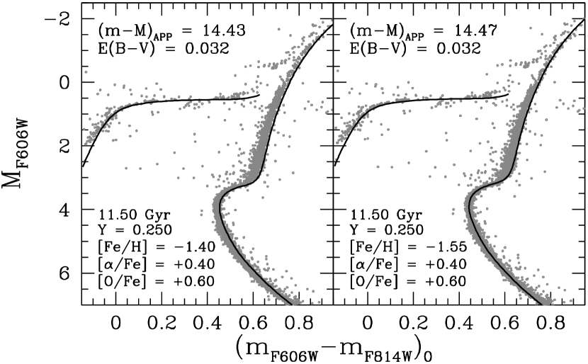
Figure 8: Similar to Fig. 6; in this case, two of many possible fits of ZAHB loci and isochrones for the indicated chemical abundances to the CMD of M 5 are shown.

The high excitation O i triplet lines are formed deep in the stellar atmospheres, where the effects of atmospheric inhomogeneities on the temperature stucture are small. According to inhomogeneous models of metal-poor halo stars, the 3D–1D, MARCS correction of oxygen abundances derived from the O i triplet is negligible (Asplund 2005, his Fig. 8).

The Fe abundance determined from Fe ii lines is practically unaffected by departures from LTE (Mashonkina et al. 2011; Lind, Bergemann, & Asplund 2012). There is, however, a small 3D–1D,MARCS correction of approximately +0.05 dex in metal-poor stars (Nissen et al. 2002, Asplund 2005).

The abundance determinations are summarized in Table 4. The statistical errors arising from uncertainties in the EWs and those of the ${T_{\rm eff}}$ and $\log\,g$ values are on the order of $\pm 0.07$ dex for $A$(O) and $\pm 0.04$ dex in the case of $A$(Fe). Systematic errors due to uncertainties in the $gf$-values, the non-LTE effects, and the 3D–1D corrections are larger: we estimate total uncertainties of $\pm 0.15$ dex for $A$(O) and $\pm 0.10$ dex for $A$(Fe). The table also lists [Fe/H] and [O/Fe] values corresponding to the solar abundances reported by Asplund et al. (2009, who give $A$(O)${}_{\odot}=8.69$ and $A$(Fe)${}_{\odot}=7.50$). As noted, [O/Fe] in HD 84937 is about 0.15 dex lower than in the other three stars, but given that the error of the differential values of [O/Fe] is $\pm 0.08$ dex (mostly due to the temperature uncertainties) this could be an accidental $2\,\sigma$ deviation. (Alternatively, the lower abundance may be due to gravitational settling, which is expected to have bigger effects on the surface abundances of turnoff stars than those on the MS or SGB; see Richard et al. 2002.)

The O and Fe abundances agree fairly well with results from recent studies. In a large survey of 825 stars in the local disk and halo, Ramírez, Allende Prieto, & Lambert (2013) derived oxygen abundances from the O i triplet lines using their own non-LTE calculations. The four stars discussed in this paper are included in their survey. The mean differences (this paper $-$ Ramírez) and rms deviations are: $\Delta\,T_{\rm eff}=30\,\pm 35$ K, $\Delta\,{\rm log}\,g=-0.02\,\pm 0.06$, $\Delta\,{\rm[Fe/H]}=-0.09\,\pm 0.05$, $\Delta\,{\rm[O/H]}=-0.05\,\pm 0.13$, and $\Delta\,{\rm[O/Fe}]=+0.04\,\pm 0.12$. The rms deviations correspond well to the estimated errors in the two studies. There seems, however, to be a significant systematic difference in the [Fe/H] values in the sense that the Ramírez et al. metallicity scale is about 0.10 dex higher than ours. On the other hand, our metal abundances agree almost exactly ($\Delta{\rm[Fe/H]}=+0.01\,\pm 0.02$) with those of Casagrande et al. (2010) and Meléndez et al. (2010), who adopted mean values of [Fe/H] from a number of recent high-resolution studies.

The oxygen abundance may also be determined from the forbidden [O i] line at 6300 Å, which is, however, very weak in spectra of metal-poor F and G dwarf stars. This line could not be detected in HD 19445 and HD 84937, but in our spectrum for HD 132475, we measured an equivalent width of $EW=1.7$ mÅ (after a small correction for the contribution of the Ni i blend (Allende Prieto, Lambert, & Asplund 2001), and in the case of HD 140283, Nissen et al. (2002) obtained $EW=0.5$ mÅ. Non-LTE corrections are negligible, but there is a significant 3D–1D correction on the order of $-0.2$ dex (see Nissen et al. 2002), because the [O i] line is formed in the upper layers of the atmosphere, where the temperature is lower in 3D models than in 1D models. Taking this into account, we derive $A$(O) = 7.60 for HD 132475 and $A$(O) = 6.95 for HD 140283. In the case of HD 132475, the oxygen abundance from the [O i] line is $\sim\!0.2$ dex lower than derived from the triplet, whereas the two O abundances happen to agree for HD 140283. As the oxygen abundances derived from the [O i] line have statistical errors on the order of $\pm 0.2$ dex due to the weakness of this line, we consider the results from the O i triplet to be more reliable.

The [O i] $\lambda\,6300$ line is of sufficient strength in metal-poor K giants to allow a precise determination of their oxygen abundances. In an extensive study of such stars, Cayrel et al. (2004) found a plateau of [O/Fe] $\simeq 0.7$ at [Fe/H] $<-2$ based on a 1D model atmosphere analyses. Applying 3D-1D corrections of $-0.1$ dex (Collet, Asplund, & Trampedach 2007) for giants, the plateau value decreases to [O/Fe] $\simeq 0.6$, in good agreement with the average ratio, [O/Fe] $=0.57$ that has been derived in this paper for the four dwarfs and subgiants.

3.3 C, N, and $\alpha$-element Abundances

The abundances of carbon and nitrogen relative to that of iron are not far from the solar ratios. From equivalent widths of C i lines near 9100 Å, we get [C/Fe] $=-0.01$ for HD 84937 and [C/Fe] $=0.08$ for HD 140283 if non-LTE corrections from Fabbian et al. (2009b) corresponding to $S_{H}=1$ are adopted. If $S_{H}=0$, these abundance ratios are decreased by 0.08 dex. In the case of HD 132475, Nissen et al. (2014) derive [C/Fe] = 0.15 from the weak C i lines at 5250 and 5380 Å. We have no data for HD 19445, but Takeda & Takada-Hidai (2013) obtained [C/Fe] $=+0.03$ from a set of infrared C i lines at 1.068–1.069 $\mu$m. Within the estimated errors, typically $\pm 0.15$ dex, all of these values are compatible with a solar C/Fe ratio. Concerning nitrogen, we note that a model-atmosphere synthesis by Israelian et al. (2004) of the NH band at 3360 Å in UVES spectra yields [N/Fe] $=0.35$ for HD 19445, $<0.0$ for HD 84937, and 0.05 for HD 140283. These values are based on 1D model atmospheres. According to Asplund (2005), large negative 3D corrections should be applied, because the NH band is formed high in the atmospheres, which decreases [N/Fe] by 0.4 to 0.5 dex. For HD 132475, we have not been able to find any determinations of the nitrogen abundance based on high-resolution spectra, but intermediate-resolution observations of the NH band yield [N/Fe] $\sim-0.5$ (Carbon et al. 1987). Hence, although the N abundances are uncertain, it is clear that none of the four stars considered here belong to the rare class of N-rich halo stars (Bessell & Norris 1982), and that nitrogen gives a negligible contribution to the total abundance of the CNO elements.

The abundances of the $\alpha$-capture elements, Mg, Si, and Ca, have been determined from one Mg i line ($\lambda 5711.1$), two Si i lines ($\lambda 6155.1$ and $\lambda 6237.3$), and eight Ca i lines in the wavelength range 6100–6440 Å. The sources of the relevant $gf$ values are Chang & Tang (1990) for Mg, Shi et al. (2009) for Si, and Smith & Raggett (1981) for Ca. Non-LTE corrections of about $+0.15$ dex for the Mg i line were adopted from Zhao & Gehren (2000), whereas the corrections for the Si and Ca lines are vanishingly small (Shi et al. 2009; Mashonkina, Korn, & Przybilla 2007). In addition, we include small 3D–1D corrections from Asplund (2005). Based on all of this, we derive the [$\alpha$/Fe] values given in Table 4 (adopting solar abundances from Asplund et al. 2009). As shown in this table, the [$\alpha$/Fe] values of HD 19445, HD 84937, and HD 132475 are close to 0.40 dex, while that for HD 140283 (0.26 dex) is lower. This may be a statistical fluctuation because the error of [$\alpha$/Fe] is on the order of $\pm 0.1$ dex. Alternatively, HD 140283 could belong to the population of ”low-$\alpha$” halo stars discovered by Nissen & Schuster (2010), although it would then be puzzling why HD 140283 does not have a lower value of [O/Fe] than the other stars. We note in this connection that the possible low [$\alpha$/Fe] has no influence on the abundance determinations: if a MARCS model with [$\alpha$/Fe] $=+0.26$ is applied instead of the canonical value of $+0.40$ dex, there is no significant change of the derived abundances.

3.4 Initial Chemical Abundances

The abundances described in the previous subsections refer to the present compositions of the stellar atmospheres. As discussed by Bond et al. (2013), the observed surface abundances should be adjusted for the effects of diffusive processes in order to yield the bulk composition of the stellar interior. (If gravitational settling is not treated, the age of HD 140283 would exceed the age of the universe as determined from Planck and WMAP observations by $\mathrel{\hbox{\raise 2.58334pt\hbox{$>$}\kern-7.3194pt\lower 2.15277pt\hbox{$\sim$}}}1.5$ Gyr.) However, it is clear from the studies by Lind et al. (2008); Nordlander et al. (2012, and references therein), and Gruyters et al. (2013) that diffusive stellar models are not able to reproduce the observed variations of the metal abundances of stars lying between the TO and the base of the giant branch in GC CMDs unless additional mixing (below envelope convection zones) is invoked to limit the efficiency of diffusion in their surface layers (also see Richard et al. 2002). In the case of NGC 6397, which has [Fe/H] $\approx-2.0$ (e.g., Carretta et al. 2009), Nordlander et al. concluded that the difference between the initial and observed metal abundances in the case of cluster subgiants with ${T_{\rm eff}}\approx 5800$ K (similar to that of HD 140283) is 0.1–0.15 dex, depending on how this extra mixing is treated. Similar, or slightly smaller, differences were obtained by Gruyters et al. in their investigation of NGC 6752 ([Fe/H] $\approx-1.55$).

Based on these findings, we decided to correct the [Fe/H] value that we determined for HD 132475 by $+0.10$ dex and those of the other three stars by $+0.15$ dex. (As mentioned in § 3.2, a larger adjustment could well be more appropriate for HD 84937.) If the same corrections are applied to the absolute abundances of all of the metals, the inferred [$m$/Fe] values remain unaffected. However, since the ages of very metal-poor subgiants, at their observed absolute magnitudes, depend primarily on their absolute oxygen abundances (see below), the adoption of increased [O/H] values by 0.1–0.15 dex does have the effect of reducing the ages derived for them by 0.3–0.5 Gyr, which is not negligible. That is, the ages of HD 132475 and HD 140283 that are derived in this study would have been higher by up to 0.5 Gyr if the aforementioned adjustments to the observed abundances had not been made.

4 Stellar Evolutionary Models

For the comparisons with observations presented below, stellar models have been computed using the version of the Victoria stellar evolution code that has been described in considerable detail by VandenBerg et al. (2012). The main differences relative to previous versions (e.g., see VandenBerg et al. 2000) are the incorporation of the latest rates for the H-burning reactions and a careful treatment of the gravitational settling of helium, along with the implementation of additional mixing below envelope convection zones (when they are present) in order to satisfy the solar and “Spite plateau” (Spite & Spite 1982) lithium abundance constraints (e.g., Richard et al. 2002). Interestingly, the net effect of these improvements on the TO luminosity versus age relations that are applicable to old Population II stars is quite small: the $\sim 10$% reduction of the TO age that occurs when diffusive processes are treated (Proffitt & VandenBerg 1991) is largely offset by a comparable increase of this quantity when recent determinations of the rate of the critical ¹⁴N$(p,\,\gamma)^{15}$O reaction (Formicola et al. 2004, Marta et al. 2008) are adopted in computations of stellar models (as first reported by Imbriani et al. 2004).

The physics improvements that have been made have much bigger consequences for the predicted temperatures of stars and the morphologies of their evolutionary tracks than for the dependence of the TO luminosity on age. However, the model effective temperature (${T_{\rm eff}}$) scale is subject to many uncertainties (including, in particular, the treatment of convection and the atmospheric boundary condition), and its accuracy can be assessed only through comparisons with empirical determinations. As shown by VandenBerg, Casagrande, & Stetson (2010, see their Fig. 10), current Victoria-Regina isochrones reproduce the locations of field halo subdwarfs that have well determined distances from Hipparcos (van Leeuwen 2007) very well if the temperatures of the latter are close to the values derived by Casagrande et al. (2010) from their calibration of the infrared-flux method (IRFM). In fact, similar success is obtained on many CMDs (also see VandenBerg et al. 2014) if color–${T_{\rm eff}}$ relations (Casagrande & VandenBerg 2014) based on the latest MARCS model atmospheres (Gustafsson et al. 2008) are used to transpose the models to the observational planes. (The same transformations are used in this study to derive bolometric corrections and colors.)

Moreover, VandenBerg et al. (2013) have shown that the same isochrones provide a close match to the shapes of GC CMDs from at least $\sim 2$ mag below the TO through to approximately the middle of the subgiant branch (SGB), independently of the assumed age and metallicity (see their Figs. 2 and 3). Indeed, this provides an argument that the errors of the predicted TO temperatures due to the neglect of metals diffusion (see footnote 7) are probably quite small. The main concern with these models is that the predicted locations of cluster RGBs appear to be somewhat too cool/red, but the primary cause of this discrepancy has not yet been identified. It is possible, for instance, that the assumption of a constant value of the mixing-length parameter, ${\alpha_{\rm MLT}}$, is at the root of this difficulty, given that calibrations of this parameter using 3D model atmospheres suggest that it should vary somewhat with ${T_{\rm eff}}$, $\log\,g$, and [Fe/H] (Trampedach & Stein 2011; Magic, Weiss, & Asplund 2014). Errors in the color transformations and the treatment of the surface boundary condition could also be contributing factors. Indeed, we suspect that it will be difficult to resolve this issue as long as the uncertainties associated with the derived temperatures and metallicities of metal-poor giants (in the field or in star clusters) remain as large as they are (typically $\sim\pm 70$ K and $\sim\pm 0.1$–0.2 dex, respectively). Worth mentioning is the fact that the aforementioned problem concerning the RGB, which has little or no impact on the ages derived in this study, is not unique to models that are generated using the Victoria code. As shown by VandenBerg et al. (2012), evolutionary tracks from the zero-age main sequence to the RGB tip (and such properties as the helium core mass at core helium ignition) are in excellent agreement with those obtained using the completely independent, very versatile MESA program (Paxton et al. 2011), when essentially the same up-to-date physics is assumed.

We note, finally, that new grids of tracks and isochrones (which will be the subject of a separate paper by D. VandenBerg et al. 2014, in preparation) are used in the following analysis. Whereas the models used by Bond et al. (2013) to derive our initial estimate of the age of HD 140283 assumed the solar mix of the metals given by Grevesse & Sauval (1998), with various enhancements to the abundances of the $\alpha$-elements (O, Ne, Mg, etc.) and then scaled to the observed [Fe/H] value, the newly computed models assume the solar metal abundances given by Asplund et al. (2009) as the base mixture. At low metallicities, the abundances of all of the $\alpha$-elements, except oxygen, are assumed to be enhanced by the fixed amount of 0.4 dex (i.e., [$m$/Fe] $=0.4$). However, because TO luminosity versus age relations are such a strong function of the oxygen abundance, which is subject to considerable uncertainties and which appears to vary to some extent from star-to-star (e.g., Fabbian et al. 2009b; Ramírez, Meléndez, & Chanamé 2012) and possibly from cluster-to-cluster, separate grids of models have been computed for [O/Fe] $=0.4,0.6,0.8$ and 1.0. Moreover, to address possible helium abundance variations, grids of evolutionary tracks have also been computed for helium mass-fraction abundances $Y=0.245$ and 0.285 (for each assumed metallicity). Fully consistent low- and high-temperature opacities for each chemical mixture have been used in the model computations.

As described by VandenBerg et al. (2014), the software developed by P. Bergbusch permits simultaneous interpolations in three chemical abundance parameters ([Fe/H], $Y$, and either [$\alpha$/Fe], if the abundances of all of the $\alpha$-elements vary together, or [O/Fe], if a constant [$m$/Fe] value is assumed for the heavier $\alpha$-elements). As a result, we have the capability to generate isochrones for very close to the preferred chemical abundances. While there will still be small differences between the assumed and actual [$m$/Fe] values for many of the metals, the effects of such differences on isochrones that are applicable to low-metallicity stars are of little consequence (see below). What is important is that we are able to treat [Fe/H], [O/Fe], and $Y$ as free parameters. (At this time, the model grids span the range in [Fe/H] from $-1.4$ to $-2.8$, though they will be extended to both lower and higher iron abundances in the coming months.)

5 The Ages of the Three Subgiants

Figure 1 compares isochrones for the indicated ages and initial chemical abundances with the observed locations of HD 84937 and HD 140283 on the $(\log{T_{\rm eff}},\,M_{V})$-diagram. The adopted $V$ magnitudes, reddenings, and the values of $M_{V}$ that correspond to the parallaxes listed in Table 2, suitably adjusted by $A_{V}=3.07\,E(B-V)$ (e.g., McCall 2004), are given in Table 5, which also lists the observed Johnson-Cousins $B-V$ and $V-I$ colors from Casagrande et al. (2010). Irrespective of whether or not the statistical Lutz-Kelker corrections (Lutz & Kelker 1973) should be applied, they are negligible for the subgiants in our sample because of the high precision of our parallax determinations ($\sigma_{\pi}/\pi\mathrel{\hbox{\raise 2.58334pt\hbox{$<$}\kern-7.74998pt\lower 2.15277pt\hbox{$\sim$}}}0.02$). For instance, using an equation provided by Hanson (1979), these corrections amount to only $-0.0023$ mag or less (in an absolute sense). Consequently, they have not been included in the tabulated absolute magnitudes.

The main reason why HD 19445 has been included in this plot is to demonstrate that isochrones satisfy the ${T_{\rm eff}}$ constraint provided by this star very well (as in the case of local subdwarfs of higher metallicity; see VandenBerg et al. 2010, 2014). For the sake of clarity, only a small segment of a 12.5 Gyr isochrone for the metallicity of HD 19445 has been plotted. Clearly, an appreciably older or younger isochrone would have served our purposes just as well given the fairly large uncertainties in the properties of HD 19445 and the small separations between isochrones of different age at $M_{V}\mathrel{\hbox{\raise 2.58334pt\hbox{$>$}\kern-7.3194pt\lower 2.15277pt\hbox{$\sim$}}}5$. Faint subdwarfs provide good tests of the predictions of stellar models and they represent one of the favored standard candles for distance determinations precisely because their properties are nearly independent of age.

HD 84937 appears to be just beginning its SGB evolution, and in fact, it is more correctly described as a TO star. At the location of HD 84937, isochrones for its observed metal abundances are more vertical than horizontal; consequently, the uncertainty of its age is due mostly to the uncertainty associated with its ${T_{\rm eff}}$ rather than that of its $M_{V}$. According to the interpolation results given in Table 6, the age of HD 84937 is 12.09 Gyr, with uncertainties of $\pm 0.14$ Gyr and $\pm 0.63$ Gyr from the vertical and horizontal error bars, respectively. The actual uncertainty will be larger than this since, in particular, the model ${T_{\rm eff}}$ scale is uncertain by at least $\sigma\,(\log{T_{\rm eff}})\sim 0.005$, which is the horizontal shift in the isochrones that is permitted by the $1\,\sigma$ error bars of HD 19445. (A further complication is the possibility that we have underestimated the effects of gravitational settling on the surface abundances of HD 84937, which would also impact the inferred age.) By comparison, the Hipparcos parallax, $\pi=13.74\pm 0.78$ mas (van Leeuwen 2007), which implies $M_{V}=3.98\pm 0.12$, would have placed this star right at the turnoff of the 12.5 Gyr isochrone for its metallicity. (Note that the tabulated masses were used to calculate the gravities which are listed in Table 4 using equation 1.)

Similar interpolations in isochrones computed for the measured abundances of HD 140283 yield an age of 14.27 Gyr, with the vertical and horizontal error bars implying age uncertainties of $\pm 0.38$ Gyr and $\pm 0.37$ Gyr, respectively (see Table 6). Because the SGB has a relatively shallow slope, the consequences of the ${T_{\rm eff}}$ uncertainty for the inferred age is much less of a concern than in the case of HD 84937, and indeed, the parallax (and hence $M_{V}$) uncertainty is the larger of these two contributors to the error budget by just a small amount. Thus, despite carrying out a new spectroscopic study of HD 140283 and using new sets of stellar models, the age of this star differs only slightly from the determination of $14.46\pm 0.31$ Gyr reported by Bond et al. (2013). This is not too surprising, however, since the values of [Fe/H] and [O/Fe] which have been derived in this investigation are quite similar to those adopted by Bond et al., and it is to be expected that the effects of small metal abundance differences in the respective isochrones will be of little consequence as long as nearly the same absolute oxygen abundance is assumed. This claim is supported by the isochrone comparisons presented in Figure 2.

In the uppermost panel of Fig. 2, the models assume the same helium and oxygen abundances ($Y=0.25$, [O/H] $=-1.70$), but different metallicities by $\delta\,$[Fe/H] $=0.2$ dex (and hence different values of [O/Fe] by the same amount). Since the [Fe/H] value represents the factor used to scale the $\log N$ abundances of all of the metals from the assumed solar mixture (with the adopted $\alpha$-element abundance enhancements taken into account) to the metallicity of interest, all of the metals other than oxygen have higher absolute abundances by 0.2 dex in the [Fe/H] $=-2.2$ isochrones than in those for [Fe/H] $=-2.4$. Despite this difference, the solid and dashed isochrones for an age of 14.0 Gyr have virtually identical TO luminosities; i.e., with a suitable horizontal shift of either of these two isochrones, they would overlay each other nearly exactly in the vicinity of the turnoff (and elsewhere, in fact). However, in this study, temperature differences are important, and the slight shift to cooler temperatures that is predicted to occur when the abundances of the metals are increased will have some consequences for the inferred age of HD 140283. Judging from the separation between the 13.5 and 14.0 Gyr isochrones that have been plotted as solid curves, a 0.2 dex error in all of the derived metal abundances (at constant [O/Fe]) would change the derived age by about 0.2 Gyr: the lower the [Fe/H] value, the higher the age. (We chose not to plot isochrones for the specific initial abundances and age that we have determined for this star, as the clarity of the figure was improved by having the model loci slightly offset from the position of HD 140283.)

The middle panel of Fig. 2 demonstrates that helium abundance uncertainties have no significant impact on the age of HD 140283 due to its fortuitous location close to the center of the SGB, where isochrones of the same age and metal abundances, but different $Y$, are virtually coincident. It is a well-known result (e.g., see Valcarce, Catelan, & Sweigart 2012; VandenBerg et al. 2012) that, at least at low metallicities, helium has only a small effect on the slope of the subgiant branch (at a fixed age), but not on the luminosity near the middle of the SGB. The fact that the helium abundance does not play a role in the ages of HD 140283 thus removes from consideration a parameter ($Y$) that is very difficult to measure in Population II stars, and which is known to vary within some GCs (e.g., NGC 2808; see Piotto et al. 2007), possibly from cluster-to-cluster, and perhaps among field halo stars as well.

In the bottom panel, the strong dependence of age on the oxygen abundance is illustrated. In this comparison, the isochrones have the same absolute abundances of all of the metals, except oxygen, which is varied by $\delta\,$[O/H] $=0.2$ dex. The case represented by the solid curves assumes [Fe/H] and [O/Fe] values which differ from those that we have derived for HD 140283 by only $+0.03$ and $+0.09$ dex, respectively. With these slight upward adjustments, the implied age of HD 140283 would decrease to 14.0 Gyr and an age of $\sim 13.5$–13.6 Gyr would be contained within the $1\,\sigma$ error bars. It is certainly well within the realm of possibility that the model temperatures are somewhat too high, which may ultimately turn out to be the main reason why our current best estimate of the age of this star is greater than the age of the universe by $\sim 0.4$ Gyr. At this point in time, we simply do not have any compelling, independent evidence that the isochrones are too hot. Regardless, HD 140283 is clearly a very old star that must have formed soon after the Big Bang.

The age of the last of the three subgiants in our sample, HD 132475, for which we have derived initial abundances corresponding to [Fe/H] $=-1.41$ and [O/Fe] $=+0.61$, is $12.56\pm 0.46$ Gyr (see Figure 3 and Table 6). This error bar takes into account only the uncertainties associated with the FGS parallax. Because the SGBs of isochrones for a fixed age have shallower slopes as the metallicity increases, the ramification of the adopted $\pm 60$ K ${T_{\rm eff}}$ uncertainty for the age of HD 132475 ($\pm 0.26$ Gyr, which is less than that due to the $M_{V}$ uncertainty by a factor of 1.8) is considerably smaller than in the case of HD 140283. These two stars apparently differ in age by $\mathrel{\hbox{\raise 2.58334pt\hbox{$>$}\kern-7.3194pt\lower 2.15277pt\hbox{$\sim$}}}1.5$ Gyr.

As discussed by Bond et al. (2013, see their Table 1), reasonable estimates of the uncertainties associated with all of the many factors that play a role in the determination of stellar ages (including, e.g., the adopted $V$ magnitudes, bolometric corrections, reddenings, and chemical abundances) would imply that the net $1\,\sigma$ error bar that should be attached to our age determinations is $\approx 0.8$ Gyr (or a little higher in the case of HD 84937). Although it seems unlikely that the physics of stellar interiors will undergo significant revisions in the coming years, since opacities (due mostly to bound-free and free-free processes involving H and He at low metallicities) and nuclear reaction rates appear to be well determined, improvements to the treatment of convection and the atmospheric boundary condition, among other things, could easily impact the model temperature scale at the level of $\delta\log{T_{\rm eff}}=\pm 0.005$–0.01. Because such variations are comparable to current uncertainties in the empirical ${T_{\rm eff}}$ scale, especially if errors in [Fe/H] are also taken into account, it will be difficult to advance our understanding of this aspect of stellar models until the observational constraints are tightened considerably.

6 Implications of the Three Subgiants for Our Understanding of GCs

In principle, HD 140283 and HD 132475 should be very good standard candles in view of their well-determined $M_{V}$ values. (HD 84937 is less useful for this purpose because it lies so close to the turnoff.) However, because they are evolved stars, the distances of objects that are derived from them will be accurate only if they share a common age and chemical composition. Nevertheless, this was believed to be the case when, e.g., VandenBerg et al. (2002, also see ) obtained $(m-M)_{V}=14.62$ for M 92 by fitting the cluster subgiants to HD 140283, on the assumption of $M_{V}=3.32\pm 0.12$ (as determined from the initial Hipparcos results by Carretta et al. 2000). (Pont et al. obtained a slightly larger apparent modulus for M 92, 14.67 mag, simply because they assumed that the reddening of HD 140283 was $E(B-V)=0.04$ mag, instead of 0.024 mag, as favored by Carretta et al.) Given the similarity of the measured [Fe/H] values of M 92 and HD 140283 and the widely held belief that the most metal deficient stars were likely to be coeval, whether found in the field or in clusters, it was not unreasonable to obtain an estimate of the distance (and age) of M 92 in this way.

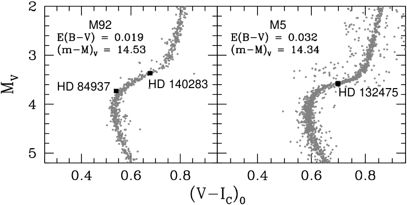
Figure 4: Fits of the M 92 and M 5 CMDs to HD 140283 and HD 132475, respectively, on the assumption that the field subgiants have the same ages and chemical abundances as their counterparts in the two globular clusters (see the text for the source of the photometric data). If reddenings from Schlafly & Finkbeiner (2011) are adopted, the derived apparent distance moduli of the two GCs have the values indicated in each panel. (HD 84937, which is more metal-rich than M 92, has been included in the left-hand panel just to illustrate where it is located relative to M 92 on the $[(V-I_{C})_{0},\,M_{V}]$ diagram. It has not been used to determine the distance modulus of M 92.)

In Figure 4, we have repeated that exercise, but using our values of $M_{V}$ for HD 140283 and HD 132475 to determine the distances to M 92 and M 5, respectively. The indicated values of $(m-M)_{V}$ correspond to the amounts that must be subtracted from the apparent magnitudes of the GC stars in order that the cluster subgiants have the same absolute magnitudes, at the same intrinsic colors, as the respective field halo subgiants. In the left-hand panel, the M 92 CMD has been fitted to the $M_{V}$ of HD 140283 that is obtained from our FGS parallax ($\pi=17.18\pm 0.26$ mas) — which actually agrees very well with the values from both the original Hipparcos catalogue ($\pi=17.44\pm 0.97$ mas, Perryman et al. 1997) and the subsequent reanalysis of the observations ($\pi=17.16\pm 0.68$ mas; van Leeuwen 2007) — together with the current best estimate of its reddening ($E(B-V)=0.004$; see § 2). This procedure yielded a value of $m-M)_{V}=14.53$ for M 92. (Note that HD 84937 played no role in this determination. It has been included in this plot just to show where this star, which is more metal rich than M 92 by $\delta$[Fe/H $\mathrel{\hbox{\raise 2.58334pt\hbox{$>$}\kern-7.3194pt\lower 2.15277pt\hbox{$\sim$}}}0.3$ dex, is located relative to the cluster turnoff.) The Johnson-Cousins photometry of HD 140283 (and HD 84937) is from Casagrande et al. (2010) while the M 92 observations were obtained from the “Photometric Standard Fields” archive made publicly available by P. B. Stetson. These data have been dereddened assuming $E(B-V)=0.019$ (from SF11) and $E(V-I)=1.3\,E(B-V)$ (e.g., Dean, Warren, & Cousins 1978).

As there is considerable support for M 92 having [Fe/H] $\approx-2.2$ (e.g., Zinn & West 1984, Carretta & Gratton 1997), its subgiants should have nearly the same $M_{V}$ as HD 140283, at the same color, provided that they have approximately the same oxygen abundance and age. (Note that the effects of diffusion on the surface chemistry of stars are largely erased by the deepening convection that occurs along the RGB; consequently, the spectroscopic abundances that are determined for GC giants will be close to their initial abundances — which are the relevant ones for our comparison. That is, cluster SGB stars that initially had [Fe/H] $\approx-2.20$ presumably have the observed surface metallicity of HD 140283 at the same evolutionary state, if diffusive processes operate at the same rates in both.) However, a value of $(m-M)_{V}$ as small as 14.53 is in conflict with most estimates. For instance, VandenBerg et al. (2013) recently derived $(m-M)_{0}=14.66$ for the true distance modulus of M 92 based on a fit of a zero-age horizontal branch (ZAHB) to the lower bound of the distribution of its HB stars. The ZAHBs presented in that study were shown to satisfy current empirical constraints on RR Lyrae luminosities (see their Fig. 10) quite well. Obviously, something is awry and, in the next subsection, we try to resolve this dilemma.

Before doing that, a few remarks are in order concerning the right-hand panel of Fig. 4. Our estimate of the initial iron abundance of HD 132475 ([Fe/H] $=-1.41$) is well within the uncertainties of many determinations of the metallicity of M 5 (e.g., Zinn & West 1984, Carretta et al. 2009). Furthermore, [O/Fe] $=0.4$–0.6 is generally found in GC stars that constitute the high oxygen end of the O–Na anticorrelation (including members of M 5; see Carretta et al. 2010, Smith et al. 2013). Since the SGB of M 5 has little vertical scatter, the total C$+$N$+$O abundance must be nearly constant, in which case, the low [O/Fe] values that are also found in most clusters arose from deep mixing along the upper RGB (e.g., Denissenkov & VandenBerg 2003) and/or the gas out of which the current stars formed had previously undergone different amounts of CNO-processing, perhaps in the AGB stars from a slightly earlier stellar generation (e.g., Gratton, Carretta, & Bragaglia 2012) or in a primordial supermassive star (Denissenkov & Hartwick 2014). In any case, M 5 appears to be chemically quite similar to HD 132475, and if the latter is used to determine the distance modulus of the former, one obtains $(m-M)_{V}=14.34$. (As in the case of M 92, Stetson’s “Photometric Standard Fields” photometry of M 5 has been plotted, the reddening is from SF11, and the source of the Johnson-Cousins $VI$ data for HD 132475 is Casagrande et al. 2010.)

Assuming the standard value of $A_{V}=3.07\,E(B-V)$, the true distance modulus of M 5 is 14.24, which agrees quite well with the value of $(m-M)_{0}=14.27$ that was obtained by VandenBerg et al. (2013) from a fit of a ZAHB to the cluster horizontal branch stars. However, the latter adopted [Fe/H] $=-1.33$ (Carretta et al. 2009) for M 5: the assumption of [Fe/H] $=-1.41$ would have resulted in a larger modulus by a few hundredths of magnitude. Still, the two independent ways of deriving the distance yield reasonably consistent results, in contrast with our findings in the case of M 92, when HD 140283 is used as a standard candle. We now turn to an investigation of this problem, though we will return to a consideration of M 5 afterwards.

6.1 The Distance and Age of M 92

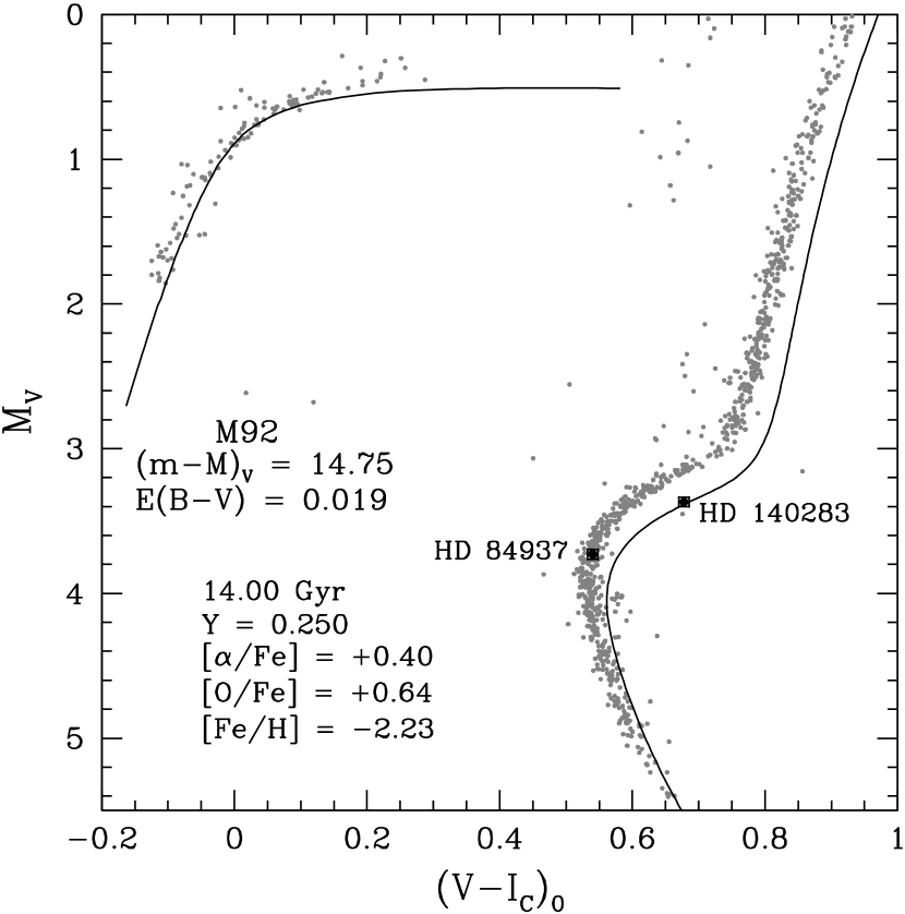
Figure 5: Similar to the left-hand panel in the previous figure; in this case, the apparent distance modulus of M 92 is based on a fit of a ZAHB to the lower bound of the distribution of cluster HB stars. If the higher value of $(m-M)_{V}$ is the more accurate determination, HD 140283 is much fainter than cluster subgiants that have the same intrinsic $V-I_{C}$ color. A 14.0 Gyr isochrone for the chemical abundances of HD 140283 has also been plotted.

Figure 5 plots the same 14.0 Gyr isochrone that appeared in Fig. 1, but on the $[(V-I)_{0},\,M_{V}]$-plane. On this CMD, the inferred age of HD 140283 is about 0.30 Gyr younger than our best estimate from the $(\log{T_{\rm eff}},\,M_{V})$-diagram, though virtually the same age that was derived in § 5 is implied by both the $B-V$ and $V-K_{S}$ colors of HD 140283 (not shown). As discussed by Casagrande & VandenBerg (2014), whose color–${T_{\rm eff}}$ relations are used throughout this investigation, uncertainties in the zero-points of the transformations at the level of 0.01–0.015 mag are easily possible (for any color index). Alternatively, it may be the observed $V-I$ color of HD 140283 that is anomalously too blue by a small amount (for whatever reason). This is a moot point. What is troubling is that the fit of a fully consistent ZAHB to the cluster counterpart in M 92 yields an apparent distance modulus, $(m-M)_{V}=14.75$, that is 0.22 mag higher than the value which is obtained by matching the cluster CMD to HD 140283 (see the previous figure). If the shorter modulus is adopted, not only would the cluster HB stars be fainter than our ZAHB models (which, as already mentioned, do a good job of satisfying empirical RR Lyrae luminosity constraints; see VandenBerg et al. 2013), but the cluster main sequence (MS) would be much fainter, at a given color, than the MS portion of the isochrone for [Fe/H] $=-2.23$ that has been plotted in Fig. 5. This is problematic because the separations between isochrones for low metallicities are predicted to be quite small at $M_{V}\mathrel{\hbox{\raise 2.58334pt\hbox{$>$}\kern-7.3194pt\lower 2.15277pt\hbox{$\sim$}}}5$ on the $V-I,\,V$ plane (see VandenBerg et al. 2010, their Fig. 11).

These difficulties are almost certainly telling us that M 92 and HD 140283 cannot have the same age — the field halo subgiant must be older — and perhaps even that they are chemically dissimilar. To examine the implications of possible age and chemical abundance differences, we have opted to fit isochrones and ZAHB loci to the $F606W,\,F814W$ photometry that was obtained by Sarajedini et al. (2007) using the ACS (Advanced Camera for Surveys) on the Hubble Space Telescope. (The same data were recently used in the determination of the ages of 55 of the GCs in their sample by VandenBerg et al. 2013.) The main reason for this choice is that a deeper and tighter CMD for M 92 can be derived from this archive than from any other publicly available source. In addition, since we intend to carry out similar fits of stellar models to the CMD of M 5, it is an important advantage of using the Sarajedini et al. observations that they represent a very homogeneous data set.

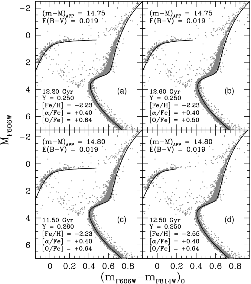
Figure 6: The age of M 92 as inferred from isochrones for the indicated chemical abundances that produce the best matches to the observed turnoff luminosity if $E(B-V)=0.019$ (from SF11) and the apparent distance moduli are based on fits of ZAHB models to the cluster HB. The models in panel (a) assume the abundances that have been derived for HD 140283, whereas those in panel (b) adopt a lower [O/Fe] value by 0.14 dex. In both of these cases, the isochrones are $\sim 0.01$–0.015 mag too red along the main sequence. No such problem is found if either a slightly higher helium abundance ($0.26$, see panel c) or a higher [Fe/H] value ($-2.55$, see panel d) is assumed. Note that the reddest ZAHB model in each panel has a mass that is identical to the turnoff mass of the best-fit isochrone: less massive ZAHB models are bluer. As discussed in the text, the redward extent of a ZAHB is a strong function of the assumed iron and oxygen abundances, especially at low [Fe/H] values.

Suppose the ZAHB-based distance is the correct one and that M 92 and HD 140283 are chemically indistinguishable. As shown in panel (a) of Figure 6, a 12.20 Gyr isochrone for the derived initial abundances of HD 140283 provides quite a good match to the MS and TO of M 92, aside from being slightly too red (by only $\approx 0.01$ mag). To make this age determination, isochrones for different ages were adjusted in the horizontal direction by whatever amount was needed in order to match the turnoff color: the one that provided the best fit to the cluster stars from $\sim 1$ mag below the TO to $\sim 0.6$ mag above it was taken to be the best estimate of the turnoff age. A thorough discussion and justification of this procedure is provided by VandenBerg et al. (2013), who obtained a higher age by about 0.5 Gyr because the models that they employed assumed slightly lower values of [Fe/H] and [O/Fe] and their ZAHB models yielded a smaller distance modulus by 0.03 mag (which, by itself, accounts for about a 0.3 Gyr age difference). If M 92 has the same [Fe/H] as HD 140283, but a somewhat lower oxygen abundance (say, [O/Fe] $=+0.50$ instead of $+0.64$), the same distance modulus is obtained, but the predicted age increases to $\approx 12.6$ Gyr (see panel b). This isochrone also follows along the red edge of the cluster CMD. To obtain an age near 13.0 Gyr, the models would need to assume [O/Fe] $\mathrel{\hbox{\raise 2.58334pt\hbox{$<$}\kern-7.74998pt\lower 2.15277pt\hbox{$\sim$}}}0.3$.

Note that the ZAHB for higher [O/Fe] extends to redder colors. In these and all similar plots presented in this paper, the mass of the reddest ZAHB model is identical to the mass at the tip of the RGB that is predicted by the isochrone which is fitted to the turnoff photometry, without taking any mass loss whatsoever into account. The intrinsic color of the reddest ZAHB star in M 92 appears to be $\approx 0.20$. At this color, the ZAHB models shown in panels (a) and (b) have masses of 0.730 and 0.748 ${\cal M_{\odot}}$, respectively, whereas the corresponding RGB tip (and TO) masses are 0.790 and 0.797 ${\cal M_{\odot}}$. Thus, relatively little mass loss appears to be necessary to explain the reddest ZAHB stars in M 92, though $>0.2{\cal M_{\odot}}$ must be lost to explain the bluest stars (assuming that mass loss is the primary cause of the dispersion in color along the HB). The decreased importance of mass loss, compared with the predictions of older models, is one of the consequences of the reduced rate of the ¹⁴N$(p,\,\gamma)^{15}$O reaction (Marta et al. 2008). As shown by Pietrinferni et al. (2010), this revision causes a ZAHB model for a fixed mass and chemical abundances to be shifted to significantly higher temperatures — an effect that is especially noticeable at low metal abundances.

The small offset between the predicted and observed MS and TO colors that are apparent in panels (a) and (b) can be eliminated if models for either a slightly higher helium abundance ($Y=0.260$ instead of 0.250) or a somewhat lower metallicity ([Fe/H] $=-2.55$ rather than $-2.23$) are overlaid onto the observed CMD (see panels c and d). To be sure, ${T_{\rm eff}}$, color, and other uncertainties are large enough that this is no more than suggestive. Still, the improved agreement leads one to wonder if VandenBerg et al. (2013) generally found it necessary to shift isochrone (but not ZAHB) colors to the blue by typically $\sim 0.02$ in their large survey of GC ages because they adopted helium abundances that were too low, or more likely, [Fe/H] values that were too high. Although $Y=0.250$ is within current uncertainties of recent determinations of the primordial abundance ($0.2485\pm 0.0016$; Komatsu et al. 2011), it is possible that a somewhat larger value is more appropriate for Population II stars — perhaps especially those found in GCs, since some processing of the gas through the AGB stars of an earlier stellar generation (see, e.g., Gratton et al. 2012) or via an initial supermassive star (Denissenkov & Hartwick 2014) is suggested by the chemical abundance variations found in them.

Insofar as the possibility that M 92 has [Fe/H] $\mathrel{\hbox{\raise 2.58334pt\hbox{$<$}\kern-7.74998pt\lower 2.15277pt\hbox{$\sim$}}}-2.5$ is concerned, we note that Roederer & Sneden (2011) have obtained [Fe/H] $=-2.70\pm 0.03$ from a spectroscopic analysis of 19 of its red giants. Similar investigations by Preston et al. (2006) and Sobeck et al. (2011) have yielded [Fe/H] $\mathrel{\hbox{\raise 2.58334pt\hbox{$<$}\kern-7.74998pt\lower 2.15277pt\hbox{$\sim$}}}-2.6$ for M 15, which has generally been found to have nearly the same iron abundance as M 92 (see, e.g., Zinn & West 1984, Carretta & Gratton 1997, Kraft & Ivans 2003). According to Roederer & Sneden (also see Sobeck et al.) the 0.3 dex larger [Fe/H] values that some of the same investigators had obtained previously for both clusters (e.g., Sneden, Pilachowshi, & Kraft 2000; Sneden et al. 2000) are due to differences in the atomic data, the adopted model atmosphere grids, and the treatment of Rayleigh scattering. Additional support for a reduced metallicity is provided in Figure 7, which compares the relative locations of the M 92 RGB and the very metal-deficient field giant HD 122563 ($\pi=4.22\pm 0.55$ mas from Hipparcos; van Leeuwen 2007) on the $[(B-V)_{0},\,M_{V}]$-diagram. HD 122563 has measured [Fe/H] values that range from $\sim-2.8$ to $\sim-2.6$ (e.g., Cayrel et al. 2004, Ramírez et al. 2010, Mashonkina et al. 2011) and it seems to have normal $\alpha$-element and oxygen abundances for its metallicity ([$\alpha$/Fe] $\approx 0.45$, Kirby & Cohen 2012; [O/Fe] $\mathrel{\hbox{\raise 2.58334pt\hbox{$>$}\kern-7.3194pt\lower 2.15277pt\hbox{$\sim$}}}0.7$ Barbuy et al. 2003); consequently, it should lie on the blue side of the cluster giant branch if M 92 has, e.g., [Fe/H] $=-2.35$ (Carretta et al. 2009).

If $V-K_{S}$ colors are plotted instead of $B-V$, the resultant comparison (not shown) looks qualitatively nearly identical. (Photometry for HD 122563 has been taken from the studies by Cayrel et al. 2004 and Creevey et al. 2012.) The main advantage of examining BV observations is that $B-V$ colors are considerably more sensitive than $V-K_{S}$ to metallicity differences at low [Fe/H] values. Whereas the 12 Gyr isochrones for [Fe/H] $=-2.8,-2.5$, and $-2.2$ that have been plotted are clearly separated from one another, they are nearly coincident on the $[(V-K_{S})_{0},\,M_{V}]$-diagram. Why HD 122563 is offset by such a large amount from M 92 giants, at the same color or at the same luminosity, is not known, but it may be that its measured parallax, which has a fairly large uncertainty, is too high. Consistency with M 92 (if the latter has [Fe/H] $\mathrel{\hbox{\raise 2.58334pt\hbox{$<$}\kern-7.74998pt\lower 2.15277pt\hbox{$\sim$}}}-2.6$) would be obtained if the correct parallax of HD 122563 were $\pi\approx 3.2$ mas, which is just within the $2\,\sigma$ error bar of the Hipparcos value.

Based on the available evidence, we are inclined to adopt [Fe/H] $=-2.5\pm 0.15$ for M 92. The error bar encompasses earlier spectroscopic determinations near $-2.4$ by, e.g., Kraft & Ivans (2003) and Carretta et al. (2009), and recent values $\mathrel{\hbox{\raise 2.58334pt\hbox{$<$}\kern-7.74998pt\lower 2.15277pt\hbox{$\sim$}}}-2.6$ that have been either derived for M 92 (Roederer & Sneden 2011) or implied by studies of M 15 (Preston et al. 2006, Sobeck et al. 2011) and HD 122563 (as discussed above). If M 92 has [Fe/H] $<-2.55$, it would need to have [O/Fe] $>0.64$ in order for our ZAHB models to provide a satisfactory match to the red end of the cluster HB. As shown in panel (d) of Fig. 6, the ZAHB model for a mass that is equal to the TO mass of the best-fit isochrone is predicted to have $(m_{F606W}-m_{F814W})_{0}=0.19$, which is just barely compatible with the cluster HB (assuming that the few HB stars with redder colors are evolved stars since they tend to be brighter than a ZAHB; see the other panels). The adoption of a lower metallicity would imply an even bluer ZAHB unless a higher absolute oxygen abundance is assumed: higher [O/H] values imply younger ages at a given TO luminosity. Our analysis suggests that M 92 is younger than 13 Gyr, and it may even be younger than 12 Gyr if its stars have a very high oxygen abundance. Pending further advances in our understanding, an age near 12.5 Gyr is our current best estimate. Thus the subgiants in M 92 appear to be different from the field subgiant, HD 140283, in having both a younger age and (probably) a lower [Fe/H] value.

Before briefly considering the RR Lyrae constraint on cluster distances, the distance and age of M 5 will be derived from fits of isochrones and ZAHBs to its CMD.

6.2 The Distance and Age of M 5

As in the case of M 92, one could produce many different fits of stellar models to the CMD of M 5 given current uncertainties in [Fe/H], [O/Fe], and $Y$, as well as those associated with the cluster distance and reddening. We have chosen to present just two of them. The left-hand panel of Figure 8 shows that a ZAHB for essentially the derived abundances of HD 132475 yields an apparent modulus of 14.43 mag, if $E(B-V)=0.032$ (from SF11), which implies a TO age of $\approx 11.5$ Gyr. The ZAHB-based true distance modulus is thus $\approx 0.10$ mag larger than that inferred from HD 132475 (see Fig. 4) — a difference that is slightly larger than the $2\,\sigma$ error bar on the $M_{V}$ of the field subgiant. Indeed, this explains why the ages that have been determined for M 5 and HD 132475 (see Fig. 3) differ by about 1 Gyr. [VandenBerg et al. (2013) also obtained an age of 11.5 Gyr for M 5 using models that assumed the solar abundances given by Grevesse & Sauval (1998) as the base mixture, with suitably enhanced $\alpha$-element abundances, and then scaled to [Fe/H] $=-1.33$ (Carretta et al. 2009). Although they found a smaller modulus by about 0.05 mag, compared with our estimate, the effects on the age of adopting slightly larger values of [Fe/H] and [O/H] in their study compensates almost exactly for this difference.]

The main difficulty with the fit to the observations in the left-hand panel is that the predicted colors for the MS and TO are too red (though by only 0.01–0.015 mag, which is well within the color uncertainties). As suggested in the previous subsection, this discrepancy may be telling us that the adopted [Fe/H] value is too high. The right-hand panel shows that the best-fit isochrone for [Fe/H] $=-1.55$ reproduces the MS and TO photometry of M 5 very well without requiring any horizontal offset. (This is obviously not a compelling argument for a reduced [Fe/H] value, but neither can one rule out this possibility given current uncertainties in metal abundance determinations.) Not unexpectedly, the same age, to within the small fitting uncertainties, is obtained because both the ZAHB and the TO luminosity at a given age become brighter as the [Fe/H] value is reduced (though not at identical rates).

However, we can make use of an additional constraint to shed some light on this issue; namely, subdwarfs in the solar neighborhood with [Fe/H] values similar to that of M 5 (and HD 132475) that also have well determined parallaxes from Hipparcos. In Figure 9, all of the subdwarfs that we have been able to identify with $M_{V}>5.0$, $\sigma_{\pi}/\pi<0.10$ (van Leeuwen 2007), and [Fe/H] values within $\pm 0.15$ dex of our determination for HD 132475 have been superimposed onto the CMD of M 5. For the latter, we have adopted $E(B-V)=0.032$ (from SF11) and two different values of the apparent distance modulus. The higher value, $(m-M)_{V}=14.44$ (left-hand panel), implies the same true distance modulus as in the left-hand panel of the previous figure when the differences in $A_{V}$ and $A_{F606W}$ (see, e.g., McCall 2004) are taken into account. The lower value, $(m-M)_{V}=14.34$ (right-hand panel) is obtained when the CMD of M 5 is fitted to HD 132475 (recall Fig. 4). The [Fe/H] values, the photometry, and the adopted reddenings of the subdwarfs have all been taken from the study by Casagrande et al. (2010), while the M 5 observations are the same as those employed in the analysis of the MARCS color–${T_{\rm eff}}$ relations by VandenBerg, Casagrande, & Stetson (2010).

It turns out that the mean [Fe/H] value of the six subdwarfs that satisfied our criteria is idential to the value that we have derived for HD 132475 (i.e., $-1.51$). (Due to diffusive effects, the initial [Fe/H] values are expected to be larger than the observed values by $\sim 0.1$ dex; recall the discussion in § 3.4.) Small blueward or redward color offsets ($<0.01$ mag) were applied to the subdwarf colors, as necessary, to compensate for the effects of differences between the observed and mean metallicities. These corrections were based on the differences in the predicted colors, at the subdwarf $M_{V}$ values, of isochrones for the observed range in [Fe/H]. Lutz-Kelker corrections have not been applied to the absolute magnitudes of the subdwarfs: they are, in any case, quite small (0.03–0.05 mag for the two brightest stars, $<0.02$ mag for the others).

Effectively, Fig. 9 is telling us that the apparent distance modulus of M 5, as derived from fits of the cluster main-sequence to the sample of subdwarf calibrators that we have considered is approximately $(m-M)_{V}=14.40$. (Although not shown, the adoption of a value as low as 14.30 or as high as 14.50 causes obvious discrepancies between the subdwarfs and the M 5 CMD.) While a common age for M 5 and HD 132475 is within the uncertainties of the subdwarf-based distance (see the right-hand panel), distance moduli based on RR Lyrae stars tend to favor values of $(m-M)_{V}\sim 14.50$ (e.g., Coppola et al. 2011). For this reason, and because the modulus based on our ZAHB models is within the uncertainties of the values derived from the subdwarf and RR Lyrae standard candles (see the next section), we consider $(m-M)_{V}=14.45$ to be our “best estimate” (rounded to the nearest 0.05 mag) of the M 5 modulus. In this case, M 5 is predicted to be $\approx 1$ Gyr younger than HD 132475.

6.3 The RR Lyrae Standard Candle

At the present time, the best empirical determination of the slope of the RR Lyrae $M_{V}$ versus [Fe/H] relation is $\Delta\,M_{V}/\Delta\,$[Fe/H] $=0.214\pm 0.047$ by Clementini et al. (2003) from their analysis of $>100$ variables in the Large Magellanic Cloud (LMC). If the true distance modulus of the LMC is 18.50, which is within the 2% uncertainty of the distance derived from eight long-period eclipsing binary members by Pietryński et al. (2013), the mean $V$ magnitude of the RR Lyraes observed by Clementini et al. ($<V_{0}>$ $=19.064\pm 0.064$ at [Fe/H] $=-1.50$) implies that their mean absolute magnitude is $M_{V}=0.564\pm 0.064$ mag at the reference metallicity. These results are plotted in Figure 10 as the open circle and the dashed line. Dotted lines have been included in this figure to illustrate the effect of adopting a steeper or shallower slope by the derived $1\,\sigma$ uncertainty of this quantity. The findings of Benedict et al. (2011), who obtained $M_{V}=0.45\pm 0.05$ from FGS parallaxes of a small sample of field RR Lyraes, and of Kollmeier et al. (2013), who derived $M_{V}=0.59\pm 0.10$ using the statistical parallax technique, are also shown.

According to M. Catelan (2014, priv. comm.), the mean apparent magnitudes of the RR Lyrae variables in M 5 and M 92 are 15.062 and 15.081, respectively. Judging from the results presented in the two previous subsections, M 5 has $(m-M)_{V}=14.45\pm 0.07$ and M 92 has $(m-M)_{V}=14.77\pm 0.07$. Moreover, [Fe/H] $=-1.40\pm 0.12$ and $-2.50\pm 0.15$ appear to be reasonable estimates of the iron abundances of M 5 and M 92, in turn, based on the available (direct and indirect) evidence. Needless to say, it is encouraging to find rather good consistency of these determinations with the empirical results obtained by Clementini et al. (2003) and Kollmeier et al. (2013), to well within their $1\,\sigma$ uncertainties, and with those reported by Benedict et al. (2011), to within $1.5\,\sigma$ (see Fig. 10). Furthermore, when ZAHB-based distance moduli are adopted, our isochrones, which have been shown to provide good fits to the local subdwarf calibrators (VandenBerg et al. 2013), are able to reproduce the observed main sequences of M 5 and M 92 to within $\sim 0.01$ mag in color (or $\sim 0.05$ mag in magnitude).

As the uncertainties associated with both the RR Lyrae and subdwarf standard candles are still rather large, it is easily possible that the distance moduli derived here are too large or too small by several hundredths of a magnitude. However, something would have to be seriously wrong with our understanding of the HB stars in M 5 and (especially) M 92 if the short distance moduli implied by HD 132475 and HD 140283, respectively, are correct. Our finding that these two field halo subgiants are significantly older than well studied GCs of similar chemical compositions seems compelling.

7 Summary

The goal of this investigation since the outset was to obtain improved ages for HD 84937, HD 132475, and HD 140283, which are the three nearest Population II subgiants with [Fe/H] $\mathrel{\hbox{\raise 2.58334pt\hbox{$<$}\kern-7.74998pt\lower 2.15277pt\hbox{$\sim$}}}-1.5$ that can be age-dated directly using trigonometric parallaxes. To this end, we have used the FGS on the Hubble Space Telescope to refine their parallaxes (§ 2), we have carried out new spectroscopic determinations of their chemical compositions (§ 3), and we have employed new sets of isochrones (§ 4) to derive our best estimates of their ages (§ 5). It turns out that these subgiants have some interesting implications for our understanding of GCs that have similar metallicities (as discussed in § 6). The main results of this study are as follows:

1. Based on 10–11 epochs of FGS observations taken between 2003 August and 2011 March, we have determined that HD 84937, HD 132475, and HD 140283 have trigonometric parallaxes $\pi=12.24\pm 0.20$, $10.18\pm 0.21$, and $17.18\pm 0.26$ mas, respectively. (By comparison, the Hipparcos parallaxes for these stars have larger uncertainties by factors of $\sim 2.5$–4; see van Leeuwen 2007.) The resultant reddening-corrected absolute magnitudes are, in turn, $M_{V}=3.730\pm 0.035$, $3.580\pm 0.045$, and $3.368\pm 0.033$.

2. From analyses of high-resolution, high S/N spectra (with non-LTE and 3D effects taken into account), we obtained [Fe/H] $=-2.08$ and [O/Fe] $=+0.44$ for HD 84937, [Fe/H] $=-1.51$ and [O/Fe] $=+0.61$ for HD 132475, and [Fe/H] $=-2.38$ and [O/Fe] $=+0.64$ for HD 140283. The measured abundances of Mg, Si, and Ca indicate that these stars have $\alpha$-element abundances similar to those typically found in extreme Population II stars ([$\alpha$/Fe] $\approx 0.4$), with the possible exception of HD 140283, for which we determined [$\alpha$/Fe] $=0.26$. The three subgiants appear to have close to solar $m$/Fe number abundance ratios of C and N.

3. Isochrones were compared with the observed locations of the subgiants on the $(\log{T_{\rm eff}},M_{V})$-diagram, resulting in ages of $12.09\pm 0.14$ Gyr for HD 84937, $12.56\pm 0.46$ Gyr for HD 132475, and $14.27\pm 0.38$ Gyr for HD 140283 — where the error bars are based solely on the parallax uncertainties. These models were generated for the observed [O/Fe] values, [$m$/Fe] $=0.4$ for the other $\alpha$-elements, and the spectroscopic determinations of [Fe/H] with an adjustment of $+0.10$ dex, in the case of HD 132475, and $+0.15$ dex in the case of the other (lower metallicity) stars, to compensate for the effects of diffusive and extra mixing processes over their lifetimes; see Nordlander et al. 2012, Gruyters et al. 2013.) The age of HD 84937 is poorly constrained because it is located just past the turnoff where isochrones are nearly vertical. The estimated 60 K $1\,\sigma$ error bar in its temperature implies $\delta$(age) $=\pm 0.63$ Gyr. In contrast, the corresponding age uncertainties for HD 132475 and HD 140283 are $\pm 0.26$ and $\pm 0.37$ Gyr, respectively. However, as discussed by Bond et al. (2013, see their Table 1), errors in the derived abundances (particularly [O/H]), the adopted $V$ magnitudes and reddenings, etc., imply $\sigma$(age) $\approx 0.8$ Gyr even for the latter two stars.

4. As first reported by Bond et al. (2013), and despite considerable additional work in the meantime, the age that we have derived for HD 140283 is slightly greater than the age of the universe as inferred from observations of the CMB by about 0.5 Gyr, and approximtely 0.7 Gyr older than the expected maximum age of Population II stars (see § 1). However, the associated $1\,\sigma$ error bars overlap. The most likely explanations for these difficulties, which would impact our results for the other subgiants as well, are (i) the absolute oxygen abundance that we have determined is too low, (ii) the adopted temperature is too low, (iii) the isochrone ${T_{\rm eff}}$ scale is too high, or some combination of these possibilities. Alternatively, it remains a remote possibility that HD 140283 truly is older than 14 Gyr, and that current estimates of the age of the universe are too low. In this regard, we note that values of the Hubble constant which have been determined in some recent investigations do not agree very well with the values deduced from CMB studies. For instance, Tammann & Reindl (2013) obtained $H_{0}=63.7\pm 2.3$ km s^-1 Mpc^-1 in their investigation of distant Type Ia supernovae, as compared with the WMAP value of $H_{0}=69.32\pm 0.80$ km s^-1 Mpc^-1 (Bennett et al. 2013). In any case, HD 140283 is a very old star that must have formed soon after the Big Bang.

5. Had we neglected the gravitational settling of helium in the stellar models that were compared with HD 140283, the age discrepancies described in the previous point would have been $>1.5$ Gyr. Thus, models that neglect this physics appear to be ruled out. Moreover, diffusive models must allow for extra mixing just below envelope convection zones in order to obtain reasonable consistency between the predicted and observed metal abundances of TO and lower RGB stars in GCs, and the chemical abundance variations along the SGB. [The difference between the observed and initial [$m$/H] value is not expected to be the same for each metal (as we have assumed) given that, e.g., some species are more affected by radiative acclerations and/or turbulent mixing than others (see Richard et al. 2002). To test diffusion physics, it is therefore important to compare the measured surface abundances of many elements with those predicted for stars in several evolutionary states. For instance, Önehag, Gustafsson, & Korn (2014) have recently found systematic differences between the observed and predicted metal abundances in stars belonging to the open cluster M 67. Even though such efforts require exceedingly careful and precise work, they should be given strong support.]

6. HD 140283 appears to be significantly ($\mathrel{\hbox{\raise 2.58334pt\hbox{$>$}\kern-7.3194pt\lower 2.15277pt\hbox{$\sim$}}}1.5$ Gyr) older than M 92 (and presumably other GCs of similar metallicities; see VandenBerg et al. 2013). If the cluster subgiants that have the same intrinsic color as HD 140283 also have the same $M_{V}$, the apparent distance modulus of M 92 would be $(m-M)_{V}\approx 14.53$. This would be completely at odds with expectations based on MS-fits to local subdwarfs or the application of the RR Lyrae standard candle (or ZAHB-based distance estimates). HD 132475 also appears to be older (by $\sim 1$ Gyr) than M 5, which is believed to have similar iron and oxygen abundances. Ages greater than $\approx 12.5$ and $\approx 11.5$ Gyr that have been derived here for M 92 and M 5, respectively, would be favored if the GCs have significantly lower oxygen abundances than those found in the two subgiants. Nonetheless, the Milky Way apparently contains field halo stars that are older than those which currently reside in its GCs.

7. Stellar evolutionary models that satisfy the subdwarf and RR Lyrae constraints to within the (still fairly large) uncertainties associated with the latter seem to provide the best fits to observed GC CMDs if the low metallicity end of the cluster [Fe/H] scale is shifted to lower values by $\sim 0.1$–0.15 dex. This possibility is supported by recent spectroscopic work on M 92 and its near [Fe/H] twin M 15, as well as the location of M 92 giants relative to that of the field giant HD 122563 ([Fe/H] $\mathrel{\hbox{\raise 2.58334pt\hbox{$<$}\kern-7.74998pt\lower 2.15277pt\hbox{$\sim$}}}-2.6$) on the $[(B-V)_{0},\,M_{V}]$-diagram.

The parallaxes reported here are likely to be supplanted later this decade by precise results from Gaia (e.g., Dopita et al. 2012). However, as we have shown, the parallax error is no longer the dominant contributor to the uncertainty in the ages of the three subgiants. In this investigation, the error bars associated with chemical abundance determinations and the empirical ${T_{\rm eff}}$ scale are comparable to or more important than distance scale uncertainties. That will continue to be the case in the coming era when accurate distances have been measured for vast numbers of stars in the extended solar neighborhood.

Figure 1: Overlay of isochrones for the indicated ages and initial chemical abundances onto the locations of HD 19445, HD 84937, and HD 140283 on the $(\log\,{T_{\rm eff}},\,M_{V})$-diagram.

Figure 2: Plot to illustrate the differences between 14.0 Gyr isochrones in which only the values of [Fe/H], $Y$, and [O/H] are varied in turn (upper, middle, and lower panels, respectively). For the cases represented as solid curves, isochrones for two ages (13.5 and 14.0 Gyr) have been plotted so that the age difference implied by the vertical separations between the two 14.0 Gyr isochrones in each panel, at the color of HD 140283, can be estimated. Ages at low metallicities are much more dependent on [O/H] than [Fe/H] or $Y$.

Figure 3: Similar to Fig. 1; in this case, the 12–13 Gyr isochrones that have been plotted are applicable to HD 132475.

Figure 7: Comparison of the HB and upper RGB of M 92, if the indicated values of $E(B-V)$ (from SF11) and $(m-M)_{V}$ (see the previous figure) are assumed, with the CMD location of the extremely metal-deficient ([Fe/H] $\mathrel{\hbox{\raise 2.58334pt\hbox{$<$}\kern-7.74998pt\lower 2.15277pt\hbox{$\sim$}}}-2.6$) field giant HD 122563. The value of $M_{V}$, and the associated error bar, that have been plotted for the latter are based on its Hipparcos parallax (van Leeuwen 2007); i.e., no Lutz-Kelker correction has been applied (see footnote 8). Also shown are 12 Gyr isochrones for [Fe/H] $=-2.8,-2.5$, and $-2.2$ (the solid curves, in the direction from left to right): each isochrone also assumes [O/Fe] $=+0.8$, though the location of the RGB does not depend on the oxygen abundance.

Figure 9: Two possible fits of the M 5 CMD to nearby subdwarfs (identified by their HD numbers) that have $M_{V}>5.0$, $\sigma_{\pi}/\pi<0.10$, and [Fe/H] values that are within $\pm 0.15$ dex of that determined for HD 132475. The vertical error bars are based solely on the parallax uncertainties (van Leeuwen 2007) while $\pm 0.01$ mag has been adopted for the horizontal error bars. The only difference between the two panels is the value of $(m-M)_{V}$ that has been assumed for M 5 (as indicated). See the text for the sources of the photometry, the metallicities, and the adopted reddenings of the subdwarfs.

Figure 10: Empirical determinations of the mean RR Lyrae luminosity and its uncertainty, at the reference [Fe/H] $=-1.50$, by Benedict et al. (2011, cross) and Clementini et al. (2003, open circle), and at [Fe/H] $=-1.59$ by Kollmeier et al. (2011, open triangle). The results by Clementini et al., whose determination of the slope of the $M_{V}$ versus [Fe/H] relation is shown as a dashed line, is tied to the true distance modulus of the LMC. For the latter, a value of 18.50 has been adopted (see Pietryński et al. 2013). The dotted lines show the impact of varying the slope by its measured uncertainty. The filled circles represent the locations of M 92 and M 5, assuming our current best estimates of their distance moduli and metallicities, and the mean apparent magnitudes of their RR Lyraes kindly provided to us by M. Catelan (2014, priv. comm.).

Table 1: Astrometric Reference Star Data

ID	RA	Dec.	$V$	$B-V$	$V-I$	Sp. Type	$\pi_{\rm est}$	$\pi_{\rm FGS}$
	(J2000)	(J2000)					(mas)	(mas)
HD 84937 Field
HD 84937-R1	09 49 12.43	+13 41 46.0	13.846	0.512	0.660	F8 V	$1.47\pm 0.29$	$1.48\pm 0.09$
HD 84937-R2	09 49 06.87	+13 41 56.6	13.706	0.621	0.721	G0 V	$1.75\pm 0.35$	$1.74\pm 0.10$
HD 84937-R3	09 48 55.11	+13 43 51.9	15.557	1.251	1.487	K7 V	$3.10\pm 0.62$	$2.70\pm 0.16$
HD 84937-R4	09 48 42.28	+13 46 26.8	11.716	1.015	1.043	K0 III	$1.12\pm 0.22$	$1.22\pm 0.07$
HD 84937-R5	09 48 33.21	+13 46 02.3	12.698	0.947	1.028	K0 IV	$0.79\pm 0.16$	$0.79\pm 0.05$
HD 84937-R6	09 48 34.24	+13 45 05.1	15.051	1.162	1.185	K1 III	$0.16\pm 0.03$	$0.16\pm 0.01$
HD 84937-R7	09 48 25.37	+13 46 57.5	14.820	0.809	0.883	K0 V	$1.70\pm 0.34$	$1.29\pm 0.06$
HD 132475 Field
HD 132475-R1	15 00 05.77	$-22$ 01 32.4	14.999	0.752	0.932	G0 V	$1.86\pm 0.37$	$1.86\pm 0.08$
HD 132475-R2	15 00 07.52	$-22$ 02 11.4	15.133	0.798	0.932	G6 V	$1.59\pm 0.32$	$1.59\pm 0.07$
HD 132475-R3	14 59 48.56	$-22$ 01 05.1	15.376	0.744	0.862	G0 V	$1.09\pm 0.21$	$1.11\pm 0.06$
HD 132475-R4	14 59 49.46	$-21$ 59 18.2	15.623	0.663	0.820	G5 V	$0.91\pm 0.18$	$0.91\pm 0.04$
HD 132475-R5	14 59 43.06	$-21$ 59 20.7	14.117	0.821	0.862	G5 V	$1.66\pm 0.33$	$1.73\pm 0.12$
HD 132475-R6	14 59 56.34	$-22$ 00 18.1	14.255	0.776	0.859	G5 V	$1.68\pm 0.34$	$1.62\pm 0.11$
HD 132475-R7	14 59 30.01	$-22$ 00 27.3	13.959	0.629	0.731	G0 V	$1.29\pm 0.26$	$1.28\pm 0.06$
HD 140283 Field
HD 140283-R1	15 43 11.66	$-10$ 55 31.7	14.254	0.761	0.864	G5 V	$1.59\pm 0.32$	$1.60\pm 0.19$
HD 140283-R2	15 54 08.74	$-10$ 54 58.3	11.949	1.041	1.133	G8 III	$1.42\pm 0.28$	$1.41\pm 0.06$
HD 140283-R3	15 42 59.53	$-10$ 55 26.3	13.174	0.812	0.887	G5 IV	$1.12\pm 0.22$	$1.15\pm 0.08$
HD 140283-R4	15 42 46.83	$-10$ 57 16.2	13.175	1.141	1.204	K0 III	$0.58\pm 0.12$	$0.56\pm 0.08$
HD 140283-R5	15 42 46.52	$-10$ 56 46.9	14.673	0.825	0.904	G5 V	$1.43\pm 0.29$	$1.41\pm 0.15$
HD 140283-VTT	15 43 08.74	$-10$ 56 58.1	16.623	1.114	1.299	K2 V	$1.50\pm 0.30$	$1.46\pm 0.11$

Table 2: Astrometric Parameters for the Halo Subgiants

Star	$\mu_{\alpha,{\rm Hipp}}$	$\mu_{\delta,{\rm Hipp}}$	$\pi_{\rm Hipp}$	$\mu_{\alpha,{\rm FGS}}$	$\mu_{\delta,{\rm FGS}}$	$\pi_{\rm FGS}$
	($\rm mas\,yr^{-1}$)	($\rm mas\,yr^{-1}$)	(mas)	($\rm mas\,yr^{-1}$)	($\rm mas\,yr^{-1}$)	(mas)
HD 84937	$+373.05\pm 0.91$	$-774.38\pm 0.33$	$13.74\pm 0.78$	$+377.85\pm 0.26$	$-772.67\pm 0.25$	$12.24\pm 0.20$
HD 132475	$-558.49\pm 0.85$	$-500.37\pm 0.68$	$10.23\pm 0.84$	$-559.50\pm 0.28$	$-503.22\pm 0.21$	$10.18\pm 0.21$
HD 140283	$-1114.93\pm 0.62$	$-304.36\pm 0.74$	$17.16\pm 0.68$	$-1111.02\pm 0.26$	$-304.76\pm 0.17$	$17.18\pm 0.26$

Table 3: Line Data, Measured Equivalent Widths, and Atmospheric LTE Abundances Derived From 1D MARCS Models

					HD 19445			HD 84937			HD 132475			HD 140283
ID	$\lambda$	$\chi_{\rm exc}$	$\log\,gf$		$EW$	$A({\rm X})$		$EW$	$A({\rm X})$		$EW$	$A({\rm X})$		$EW$	$A({\rm X})$
	(Å)	(eV)			(mÅ   )			(mÅ)			(mÅ)			(mÅ)
O i	7771.95	9.15	0.37		13.9	7.36		20.8	7.29		33.5	7.98		9.0	7.14
O i	7774.18	9.15	0.22		9.5	7.31		14.5	7.22		26.6	7.96		6.2	7.09
O i	7775.40	9.15	0.00		7.0	7.38		9.1	7.20		17.1	7.90		3.7	7.07
Fe ii	5197.58	3.23	$-$2.22					13.4	5.34		40.9	5.92		10.2	5.01
Fe ii	5234.63	3.22	$-$2.18					15.9	5.38		44.7	5.95		12.7	5.07
Fe ii	5264.81	3.33	$-$3.13					2.4	5.52		10.5	6.09		1.8	5.22
Fe ii	5284.11	2.89	$-$3.11					4.1	5.35		17.9	5.92		3.2	5.02
Fe ii	5325.56	3.22	$-$3.16					2.1	5.39		8.8	5.93		1.7	5.11
Fe ii	5414.08	3.22	$-$3.58								3.6	5.93
Fe ii	5425.26	3.20	$-$3.22					2.0	5.41		8.6	5.95		1.4	5.06
Fe ii	5534.85	3.24	$-$2.75					4.8	5.36		19.0	5.92		4.3	5.13
Fe ii	6084.11	3.20	$-$3.79								2.5	5.93
Fe ii	6149.25	3.89	$-$2.69		1.2	5.38		1.9	5.44		5.6	5.87		1.1	5.07
Fe ii	6238.39	3.89	$-$2.60		1.8	5.46		1.6	5.28		7.9	5.94
Fe ii	6247.56	3.89	$-$2.30		3.2	5.42		3.5	5.32		14.2	5.93		2.1	4.96
Fe ii	6432.68	2.89	$-$3.57		1.6	5.44		1.4	5.29		7.6	5.90		1.4	5.06
Fe ii	6456.39	3.90	$-$2.05		5.3	5.40		6.0	5.33					4.2	5.03

Table 4: Atmospheric Parameters and Observed Elemental Abundances

Star	$T_{\rm eff}$	$\log\,g$	$A({\rm O})$	$A({\rm O})$	$A({\rm Fe})$	$A({\rm Fe})$	[Fe/H]	[O/Fe]	[$\alpha$/Fe]
			(1D,LTE)	(3D,NLTE)	(1D,LTE)	(3D,NLTE)
HD 19445	6136 K	4.43	7.35	7.24	5.42	5.47	$-2.03$	0.58	0.39
HD 84937	6408	4.05	7.24	7.05	5.37	5.42	$-2.08$	0.44	0.38
HD 132475	5746	3.80	7.95	7.79	5.94	5.99	$-1.51$	0.61	0.45
HD 140283	5797	3.70	7.10	6.95	5.07	5.12	$-2.38$	0.64	0.26

Table 5: Photometry, Reddenings, and Absolute Magnitudes

Star		$V$	$B-V$	$V-I$	$E(B-V)$		$M_{V}$
HD 84937		8.306	0.396	0.547	0.005		$3.730\pm 0.035$
HD 132475		8.563	0.537	0.708	0.007		$3.580\pm 0.045$
HD 140283		7.205	0.487	0.683	0.004		$3.368\pm 0.033$

Table 6: Masses and Ages

Star	${\cal M}/{\cal M_{\odot}}$	Age	$\delta$(Age)	$\delta$(Age)
		(Gyr)	(Gyr)	(Gyr)
HD 84937	0.78	12.09	$\pm 0.14$	$\pm 0.63$
HD 132475	0.80	12.56	$\pm 0.46$	$\pm 0.26$
HD 140283	0.75	14.27	$\pm 0.38$	$\pm 0.37$

References

- Ade et al. (2013) Ade, P. A. R., Aghanim, N., Armitage-Caplan, C., et al. 2013, arXiv:1303.5076
- Allende Prieto, Lambert, & Asplund (2001) Allende Prieto, C., Lambert, D. L., & Asplund, M. 2001, ApJL, 556, L63
- Alves-Brito et al. (2010) Alves-Brito, A., Meléndez, J., Asplund, M., Ramírez, I., and Yong, D. 2010, A&A, 513, A35
- Asplund (2005) Asplund, M. 2005, ARA&A, 43, 481
- Asplund et al. (2009) Asplund, M., Grevesse, N., Sauval, A. J., & Scott, P. 2009, ARA&A, 47, 481
- Asplund et al. (2006) Asplund, M., Lambert, D. L., Nissen, P. E., Primas, F., & Smith, V. V. 2006, ApJ, 644, 229
- Barbuy et al. (2003) Barbuy, B., Meléndez, J., Spite, M., et al. 2003, ApJ, 588, 1072
- Barklem (2007) Barklem, P. S. 2007, A&A, 462, 781
- Benedict et al. (2011) Benedict, G. F., McArthur, B. E., Feast, M. W., et al. 2011, AJ, 142, 187
- Benedict et al. (2009) Benedict, G. F., McArthur, B. E., Napiwotzki, R., et al. 2009, AJ, 138, 1969
- Bennett et al. (2013) Bennett, C. L., Larson, D., Weiland, J. L., et al. 2013, ApJS, 208, 20
- Bergemann (2008) Bergemann, M. 2008, Phys. Scr., 133, 014013
- Bessell (2007) Bessell, M. S. 2007, PASP, 119, 605
- Bessell & Norris (1982) Bessell, M. S., & Norris, J. 1982, ApJL, 263, L29
- Bond & MacConnell (1971) Bond, H. E., & MacConnell, D. J. 1971, ApJ, 165, 51
- Bond et al. (2013) Bond, H. E., Nelan, E. P., VandenBerg, D. A., Schaefer, G. H., & Harmer, D. 2013, ApJL, 765, L12
- Carbon et al. (1987) Carbon, D. F., Barbuy, B., Kraft, R., Friel, E. D., & Suntzeff, N. 1987, PASP, 99, 335
- Carretta et al. (2009) Carretta, E., Bragaglia, A., Gratton, R. G., D’Orazi, V., & Lucatello, S. 2009, A&A, 508, 695
- Carretta et al. (2010) Carretta, E., Bragaglia, A., Gratton, R. G., Recio-Blanco, A., Lucatello, S., D’Orazi, V., & Cassisi, S. 2010, A&A, 516, A55
- Carretta & Gratton (1997) Carretta, E., & Gratton, R. G. 1997, A&AS, 121, 95
- Carretta et al. (2000) Carretta, E., Gratton, R. G., Clementini, G., & Fusi Pecci, F. 2000, ApJ, 533, 215
- Casagrande et al. (2010) Casagrande, L., Ramírez, I., Meléndez, J., Bessell, M., & Asplund, M. 2010, A&A, 512, A54
- Casagrande & VandenBerg (2014) Casagrande, L., & VandenBerg, D. A. 2014, MNRAS, in press
- Cayrel et al. (2004) Cayrel, R., Depagne, E., Spite, M., et al. 2004, A&A, 416, 1117
- Chang & Tang (1990) Chang, T. N., & Tang, X. 1990, JQSRT, 43, 407
- Clementini et al. (2003) Clementini, G., Gratton, R. G., Bragaglia, A., Carretta, E., Di Fabrizio, L., & Maio, M. 2003, AJ, 125, 1309
- Collet, Asplund, & Trampedach (2007) Collet, R., Asplund, M., & Trampedach, R. 2007, A&A, 469, 687
- Coppola et al. (2011) Coppola, G., Dall’Ora, M., Ripepi, V., et al. 2011, MNRAS, 416, 1056
- Creevey et al. (2012) Creevey, O. L., Thévenin, F., Boyajian, T. S., et al. 2012, A&A, 545, A17
- Dean, Warren, & Cousins (1978) Dean, J. F., Warren, P. R., & Cousins, A. W. J. 1978, MNRAS, 183, 569
- Dekker et al. (2000) Dekker, H., D’Odorico, S., Kaufer, A., Delabre, B., & Kotzlowski, H. 2000, Proc. SPIE, 4008, 434
- Denissenkov & Hartwick (2014) Denissenkov, P., & Hartwick, F. D. A. 2014, MNRASL, 437, L21
- Denissenkov & VandenBerg (2003) Denissenkov, P., & VandenBerg, D. A. 2003, ApJ, 593, 509
- di Cecco et al. (2010) di Cecco, A., Becucci, R., Bono, G., et al. 2010, PASP, 122, 991
- Dopita et al. (2012) Dopita, M. A., Marconi, M., Clementini, G., & Brocato, E. 2012, ApSS, 341, 1
- Drawin (1968) Drawin, H.-W. 1968, Z. für Physik, 211, 404
- Dotter et al. (2010) Dotter, A., Sarajedini, A., Anderson, J., et al. 2010, ApJ, 708, 698
- Fabbian et al. (2009a) Fabbian, D., Asplund, M., Barklem, P. S., Carlsson, M., & Kiselman, D. 2009a, A&A, 500, 1221
- Fabbian et al. (2009b) Fabbian, D., Nissen, P. E., Asplund, M., Pettini, M., & Akerman, C. 2009b, A&A, 500, 1143
- Formicola et al. (2004) Formicola, A., Imbriani, G., Costantini, H., et al. 2004, Phys. Let. B, 591, 61
- Gehren et al. (2004) Gehren, T., Liang, Y. C., Shi, J. R., Zhang, H. W., & Zhao, G. 2004, A&A, 413, 1045
- González Hernández & Bonifacio (2009) González Hernández, J. I., & Bonifacio, P. 2009, A&A, 497, 497
- Gratton, Carretta, & Bragaglia (2012) Gratton, R. G., Carretta, E., & Bragaglia, A. 2012, A&AR, 20, 50
- Grevesse & Sauval (1998) Grevesse, N., & Sauval, A. J. 1998, Sp. Sci. Rev., 85, 161
- Gruyters et al. (2013) Gruyters, P., Korn, A. J., Richard, O., et al. 2013, A&A, 555, A31
- Gustafsson et al. (2008) Gustafsson, B., Edvardsson, B., Eriksson, K., et al. 2008, A&A, 486, 951
- Hansen et al. (2013) Hansen, B. M. S., Kalirai, J. S., Anderson, J., et al. 2013, Nature, 500, 51
- Hanson (1979) Hanson, R. B. 1979, MNRAS, 186, 875
- Hibbert et al. (1991) Hibbert, A., Biémont, E., Godefroid, M., & Vaeck, N. 1991, J. Phys. B, 24, 3943
- Imbriani et al. (2004) Imbriani, G., Costantini, H., Formicola, A., et al. 2004, A&A, 420, 625
- Israelian et al. (2004) Israelian, G., Ecuvillon, A., Rebolo, R., et al. 2004, A&A, 421, 469
- Jeffreys, Fitzpatrick, & McArthur (1988) Jefferys, W. H., Fitzpatrick, M. J., & McArthur, B. E. 1988, Celestial Mechanics, 41, 39
- Jonsell et al. (2005) Jonsell, K., Edvardsson, B., Gustafsson, B., Magain, P., Nissen, P. E., & Asplund, M. 2005, A&A, 440, 321
- Kirby & Cohen (2012) Kirby, E. N., & Cohen, J. G. 2012, AJ, 144, 168
- Kollmeier et al. (2013) Kollmeier, J. A., Szczygiel, D. M., Burns, C. R., et al. 2013, ApJ, 775, 57
- Komatsu et al. (2011) Komatsu, E., Smith, K. M., Dunkley, J., et al. 2011, ApJS, 192, 18
- Kraft & Ivans (2003) Kraft, R. P., & Ivans, I. I. 2003, PASP, 115, 143
- Landolt (1992) Landolt, A. U. 1992, AJ, 104, 340
- Lind, Bergemann, & Asplund (2012) Lind, K., Bergemann, M., & Asplund, M. 2012, MNRAS, 427, 50
- Lind et al. (2008) Lind, K., Korn, A. J., Barklem, P. S., & Grundahl, F. 2008, A&A, 490, 777
- Lutz & Kelker (1973) Lutz, T. E., & Kelker, D. H. 1973, PASP, 85, 573
- Magic, Weiss, & Asplund (2014) Magic, Z., Weiss, A., & Asplund, M. 2014, astro-ph: 1403.1062
- Marta et al. (2008) Marta, M., Formicola, A., Gyürky, Gy., et al. 2008, Phys. Rev. C, 78, 2802
- Mashonkina et al. (2011) Mashonkina, L., Gehren, T., Shi, J.-R., Korn, A. J., & Grupp, F. 2011, A&A, 528, A87
- Mashonkina, Korn, & Przybilla (2007) Mashonkina, L., Korn, A. J., & Przybilla, N. 2007, A&A, 461, 261
- Mayor et al. (2003) Mayor, M., Pepe, F., Queloz, D., et al. 2003, The Messenger, 114, 20
- McCall (2004) McCall, M. L. 2004, AJ, 128, 2144
- Meléndez & Barbuy (2009) Meléndez, J., & Barbuy, B. 2009, A&A, 497, 611
- Meléndez et al. (2010) Meléndez, J., Casagrande, L., Ramírez, I., Asplund, M., & Schuster, W. J. 2010, A&A, 515, L3
- Melis et al. (2013) Melis, C., Reid, M. J., Mioduszewski, A. J., Stauffer, J. R., & Bower, G. C. 2013, IAU Symposium, 289, 60
- Metcalfe et al. (2010) Metcalfe, T. S., Monteiro, M. J. P. F. G., Thompson, M. J., et al. 2010, ApJ, 723, 1583
- Nelan & Bond (2013) Nelan, E. P., & Bond, H. E. 2013, ApJ, 773, L26
- Nelan & Makidon (2002) Nelan, E., & Makidon, R. 2002, FGS Data Handbook, Version 4.0 (Baltimore: STScI)
- Nissen et al. (2007) Nissen, P. E., Akerman, C., Asplund, M., et al. 2007, A&A, 469, 319
- Nissen et al. (2004) Nissen, P. E., Chen, Y. Q., Asplund, M., & Pettini, M. 2004, A&A, 415, 993
- Nissen et al. (2014) Nissen, P. E., Chen, Y. Q., Carigi, L., Schuster, W. J., & Zhao, G. 2014, arXiv: 1406.5218
- Nissen et al. (2002) Nissen, P. E., Primas, F., Asplund, M., & Lambert, E. L. 2002, A&A, 390, 235
- Nissen & Schuster (2010) Nissen, P. E., & Schuster, W. J. 2010, A&A, 511, L10
- Önehag, Gustafsson, & Korn (2014) Önehag, A., Gustafsson, B., & Korn, A. 2014, A&A, 562, A102
- Nordlander et al. (2012) Nordlander, T., Korn, A. J., Richard, O., & Lind, K. 2012, ApJ, 753, 48
- Paxton et al. (2011) Paxton, B., Bildsten, L., Dotter, A., Herwig, F., Lesaffre, P., & Timmes, F. 2011, ApJS, 192, 3
- Pereira, Asplund, & Kiselman (2009) Pereira, T. M. D., Asplund, M., & Kiselman, D. 2009, A&A, 508, 1403
- Perryman (2009) Perryman, M. 2009, Astronomical Applications of Astrometry: Ten Years of Exploitation of the Hipparcos Satellite Data (Cambridge: Cambridge Univ. Press)
- Perryman et al. (1997) Perryman, M. A. C., Lindegren, L., Kovalevsky, J., et al. 1997, A&A, 323, L49
- Pietrinferni et al. (2010) Pietrinferni, A., Cassisi, S., & Salaris, M. 2010, A&A, 522, A76
- Pietryński et al. (2013) Pietryński, G., Graczyk, D., Gieren, N., et al. 2013, Nature, 495, 76
- Piotto et al. (2007) Piotto, G., Bedin, L. R., Anderson, J., et al. 2007, ApJL, 661, L53
- Pont et al. (1998) Pont, F., Mayor, F., Turon, C., & VandenBerg, D. A. 1998, A&A, 329, 87
- Preston et al. (2006) Preston, G. W., Sneden, C., Thompson, I. B., Shectman, S. A., & Burley, G. S. 2006, AJ, 132, 85
- Proffitt & VandenBerg (1991) Proffitt, C. R., & VandenBerg, D. A. 1991, ApJS, 77, 473
- Ramírez, Allende Prieto, & Lambert (2013) Ramírez, I., Allende Prieto, C., & Lambert, D. L. 2013, 764, 78
- Ramírez et al. (2010) Ramírez, I., Collet, R., Lambert, D. L., Allende Prieto, C., & Asplund, M. 2010, ApJ, 725, L223
- Ramírez, Meléndez, & Chanamé (2012) Ramírez, I., Meléndez, J., & Chanamé, J. 2012, ApJ, 757, 164
- Richard et al. (2002) Richard, O., Michaud, G., Richer, J., Turcotte, S., Turck-Chièze, S., & VandenBerg, D. A. 2002, ApJ, 568, 979
- Ritter et al. (2012) Ritter, J. S., Safranek-Shrader, C., Gnat, O., Milosavljević, M., & Bromm, V. 2012, ApJ, 761, 56
- Roederer & Sneden (2011) Roederer, I. U., & Sneden, C. 2011, AJ, 142, 22
- Roeser, Demleitner, & Shilbach (2010) Roeser, S., Demleitner, M., & Schilbach, E. 2010, AJ, 139, 2440
- Safranek-Shrader, Milosavljević, & Bromm (2014) Safranek-Shrader, C., Milosavljević, M., & Bromm, V. 2014, MNRASL, 440, L76
- Sandquist (2004) Sandquist, E. L. 2004, MNRAS, 347, 101
- Sarajedini et al. (2007) Sarajedini, A., Bedin, L. R., Chaboyer, B., et al. 2007, AJ, 133, 1658
- Schlafly & Finkbeiner (2011) Schlafy, E. F., & Finkbeiner, D. P. 2011, ApJ, 737, 103 (SF11)
- Shi et al. (2009) Shi, J. R., Gehren, T., Mashonkina, L., & Zhao, G. 2009, A&A, 503, 533
- Smith et al. (2013) Smith, G. H., Modi, P. N., & Hamren, K. 2013, PASP, 125, 1287
- Smith & Raggett (1981) Smith, G., & Raggett, D. St. J. 1981, J. Phys. B., 14, 4015
- Sneden et al. (2000) Sneden, C., Johnson, J., Kraft, R. P., Smith, G. H., Cowan, J. J., & Bolte, M. 2000, ApJ, 536, L85
- Sneden, Pilachowshi, & Kraft (2000) Sneden, C., Pilachowski, C. A., & Kraft, R. P. 2000, AJ, 120, 1351
- Sobeck et al. (2011) Sobeck, J. A., Kraft, R. P., Sneden, C., et al. 2011, AJ, 141, 175
- Soderblom et al. (2005) Soderblom, D. R., Nelan, E., Benedict, G. F., et al. 2005, AJ, 129, 1616
- Spergel et al. (2003) Spergel, D. N., Verde, L., Peiris, H. V., et al. 2003, ApJS, 148, 175.
- Spite & Spite (1982) Spite, F., & Spite, M. 1982, A&A, 115, 357
- Takeda & Takada-Hidai (2013) Takeda, Y., & Takada-Hidai, M. 2013, PASJ, 65, 65
- Tammann & Reindl (2013) Tammann, G. A., & Reindl, B. 2013, A&A, 549, A136
- Trampedach & Stein (2011) Trampedach, R., & Stein, R. F. 2011, ApJ, 731, 78
- Valcarce, Catelan, & Sweigart (2012) Valcarce, A. A. R., Catelan, M., & Sweigart, A. V. 2012, A&A, 547, A5
- VandenBerg (2000) VandenBerg, D. A. 2000, ApJS, 129, 315
- VandenBerg et al. (2012) VandenBerg, D. A., Bergbusch, P. A., Dotter, A., et al. 2012, ApJ, 755, 15
- VandenBerg et al. (2014) VandenBerg, D. A., Bergbusch, P. A., Ferguson, J. W., & Edvardsson, B. 2014, ApJ, submitted
- VandenBerg, Casagrande, & Stetson (2010) VandenBerg, D. A., Casagrande, L., & Stetson, P. B. 2010, AJ, 140, 1020
- VandenBerg et al. (2013) VandenBerg, D. A., Brogaard, K., Leaman, R., & Casagrande, L. 2013, ApJ, 775, 134
- VandenBerg et al. (2002) VandenBerg, D. A., Richard, O., Michaud, G., & Richer, J. 2002, ApJ, 571, 487
- VandenBerg et al. (2000) VandenBerg, D. A., Swenson, F. J., Rogers, F. J., Iglesias, C. A., & Alexander, D. R. 2000, ApJ, 532, 430
- van Leeuwen (2007) van Leeuwen, F. 2007, A&A, 474, 653
- Zacharias et al. (2013) Zacharias, N., Finch, C. T., Girard, T. M., et al. 2013, AJ, 145, 44
- Zhao & Gehren (2000) Zhao, G., & Gehren, T. 2000, A&A, 362, 1077
- Zinn & West (1984) Zinn, R., & West, M. J. 1984, ApJS, 55, 45