Theory of adiabatic quantum control in the presence of cavity-photon shot noise

Christopher Chamberland
Department of Physics
McGill University, Montreal

March 2014

A thesis submitted to McGill University in partial fulfillment of the requirements of the degree of M.Sc.

© Christopher Chamberland 2014

À mes parents, à Marie-Michelle et à mon oncle Claude.

Abstract

Many areas of physics rely upon adiabatic state transfer protocols, allowing a quantum state to be moved between different physical systems for storage and retrieval or state manipulation. However, these state-transfer protocols suffer from dephasing and dissipation. In this thesis we go beyond the standard open-systems treatment of quantum dissipation allowing us to consider non-Markovian environments. We use adiabatic perturbation theory in order to give analytic descriptions for various quantum state-transfer protocols. The leading-order corrections will give rise to additional terms adding to the geometric phase preventing us from achieving a perfect fidelity. We obtain analytical descriptions for the effects of the geometric phase in non-Markovian regimes. The Markovian regime is usually treated by solving a standard Bloch-Redfield master equation, while in the non-Markovian regime, we perform a secular approximation allowing us to obtain a solution to the density matrix without solving master equations. This solution contains all the relevant phase information for our state-transfer protocol. After developing the general theoretical tools, we apply our methods to adiabatic state transfer between a four-level atom in a driven cavity. We explicitly consider dephasing effects due to unavoidable photon shot noise and give a protocol for performing a phase gate. These results will be useful to ongoing experiments in circuit quantum electrodynamics (QED) systems.

Résumé

Plusieurs domaine de la physique ce fit sur des protocoles adiabatique de transfert d’état, permettant un état quantique de se déplacer entre diffèrent système physique afin de les emmagasiner, les récupéré ou de les manipuler. Par contre, ces protocoles de transferts d’état souffrent du phénomène de déphasage et de dissipation. Dans ce mémoire, nous allons au-delà des traitements standards de système ouverts décrivant la dissipation quantique nous permettant de considérer des environnements non-Markoviens. Nous utilisons la théorie de perturbation adiabatique afin de donner une description analytique à plusieurs protocoles de transfert quantique. Les corrections d’ordres principaux donnent lieu à une phase géométrique de système ouvert, ce qui nous empêche d’atteindre une fidélité parfaite. Nous obtenons une description analytique pour les effets de phase géométrique dans des régimes non-Markovien. Les régimes Markovien sont habituellement traités en trouvant une solution à une équation de maitresse Bloch-Redfield, tandis que pour les régimes non-Markovien, nous allons performer une approximation séculaire nous permettant d’obtenir une solution exacte de la matrice de densité qui contient toute l’information de phase pertinente pour nôtre protocole de transfert d’état. Après avoir développé les outils théoriques généraux, nous allons appliquer nos méthodes à un transfert d’état adiabatique entre les états d’un atom à quatre niveau dans une cavité entraînée. Nous considérons explicitement les effets de déphasage du au bruit photonique inévitable. Ces résultats seront utiles pour des expériences en cours dans des systèmes de circuits QED.

Chapter 1 Introduction

 

Quantum state transfer arises when one would like to transfer a quantum state from one system to another with the highest possible fidelity. There are many state-transfer protocols that are of practical significance. For example, if one is interested in building a secure quantum system for private communication or for long-distance quantum communication, it is necessary to transfer information between quantum-memory atoms and photons [key-1, key-2, key-3, key-4, key-5, key-6]. In other situations, it is crucial to be able to preserve a quantum state for as long as possible in order to trade states back and fourth between an ensemble of atoms and photons [key-7, key-8, key-9, key-10, key-11, key-12, key-13]. Quantum state transfer can also lead to striking results. For instance, when applied to quantum-logic clocks, they become so precise that they are able to keep time to within 1 second every 3.7 billion years [key-14]. In reality, when one performs a state-transfer protocol, the quantum systems under consideration are never completely isolated from an exterior environment. Consequently, regardless of which state-transfer protocol is being employed, one will always be faced with the challenge of fighting decoherence.

During the early days of quantum mechanics, the adiabatic theorem was a perturbative tool that was developed to deal with slowly-varying time-dependent Hamiltonians [key-15, key-16]. The Hamiltonian $H\left(t\right)$ must vary slowly compared to internal time scales of the system quantified by a dimensionless parameter $A$. For example, the parameter $A$ for a spin-half coupled to a time-dependent magnetic field would be $Bt_{p}$ where $t_{p}$ is the total time it takes the magnetic field to complete a closed loop trajectory in 3-D space [key-29]. To leading order in adiabatic perturbation theory, the instantaneous eigenstates of the Hamiltonian acquire a geometric phase (along with its usual dynamical phase). The term “geometric phase” comes from the fact that this phase depends on the path traversed by the system in Hilbert space but not on the time to traverse the path [key-17]. Recently, it has been shown that in the framework of quantum information and quantum computation, the geometric phase is robust in the presence of some sources of decoherence [key-18, key-19, key-20, key-21]. Thus, it may be useful to take advantage of this robustness to perform a phase gate in the presence of a dissipative quantum system. On the other hand, corrections to the geometric phase in the presence of a dissipative environment will be the leading source preventing one from doing a state-transfer protocol with perfect fidelity. Given these considerations, it is of paramount importance to study geometric phases for open quantum systems. Many authors [key-22, key-23, key-24, key-25, key-26, key-27, key-28, key-29] have considered geometric phases for systems coupled to classical or quantum environments. The authors of [key-29] consider a spin-1/2 system which is both subject to a slowly-varying magnetic field and weakly coupled to a dissipative environment (which the authors choose to be quantum). The authors obtained a modification to the closed-system geometric phase due to the coupling to the environment and found that this phase is also geometrical. However, the authors’ results are limited by the fact that they consider only weak dissipation and an environment giving rise to Markovian evolution. In this thesis, we develop a general theory that gives rise to non-Markovian evolution by performing a secular approximation following the criteria of [key-30]. As was shown in [key-30], performing a secular approximation on time-dependent systems can often be problematic and must be done with care. Consequently, we will go into some detail in order to ensure that the secular approximation is done correctly. Given that our main motivation is to perform a phase gate under a quantum state-transfer protocol while minimizing dephasing effects, we will develop our theory under the framework of a Stimulated Raman Adiabatic Passage (STIRAP) applied to a tripod system (Fig. 2.2.1). A STIRAP system is an adiabatic process that is efficient at transferring population in a three-level system [key-31, key-32, key-33, key-34, key-35, key-36, key-37, key-38]. When applied to a tripod system, one now deals with four levels (instead of three) allowing the possibility to transfer population amongst the two ground state levels (the levels spacing $\left.|g_{1}\right\rangle$ and$\left.|g_{2}\right\rangle$ in Fig. 2.2.1). Our task will be twofold. First we will perform a state-transfer protocol in the presence of a dissipative environment. Secondly, we will perform a phase-gate state-transfer protocol by transferring quantum information between the four-level system the presence of a dissipative environment. The fourth level (the state $\left.|0\right\rangle$ in Fig. 2.2.1) in our tripod system will act as a spectator state meaning that no driving terms will couple it to an excited state (unlike the two other levels of the tripod system which are coupled to an excited state via time-dependent classical fields). In this case, the spectator state will not acquire a geometric phase. However, the other instantaneous eigenstates of our system will acquire an environment-induced (as well as a closed-system) geometric phase. It will thus be crucial to understand how non-Markovian environments modify the closed-system geometric phase.

In chapter 2 we give an overview of adiabatic perturbation theory and of the dynamics of the geometric phase. We will then apply adiabatic perturbation theory to describe the closed-system four-level adiabatic state-transfer protocol described above. We will also show how all the phase information is encoded in the off-diagonal components of the density matrix and how our state-transfer protocol can be described in the language of density matrices. We will conclude chapter 2 by giving an overview of cavity-photon shot noise. In chapter 3, we develop a theory allowing us to calculate dephasing effects in our state-transfer protocol for the case where the system is coupled to a quantum dissipative bath. We will do this by performing a secular approximation in a superadiabatic basis allowing us to obtain the relevant off-diagonal component of the density matrix. We will conclude chapter 3 by applying our theory to a system of independent bosonic modes coupled to our four-level system. In chapter 4, we will apply our methods to adiabatic state transfer of a four-level system in a driven cavity. We will explicitly consider dephasing effects due to unavoidable photon shot noise. Once the dephasing effects have been accounted for, we will show how it is possible to perform a phase gate by choosing specific functional forms for the phase difference between the two laser fields driving the cavity. These results will be useful to ongoing experiments in circuit QED systems.

Chapter 2 Adiabatic evolution and noise

 

2.1. Adiabatic approximation and the Berry’s phase

When dealing with physical systems where the Hamiltonian takes on an explicit time dependence, it is often very difficult to solve the Schroedinger equation exactly. One must often approach the problem using perturbative techniques to have some hope of getting analytical results. The adiabatic approximation is very useful for cases where the Hamiltonian changes slowly in time. However, at this stage, one must correctly define what we mean by changing “slowly in time”. To address this issue on analytical grounds, we can start by looking at the energy eigenvalues of the Hamiltonian. For a fixed value of time, it is always possible to obtain the energy spectrum of the Hamiltonian which depends on a set of parameters. Consequently, when we say that the Hamiltonian changes slowly in time, we mean that the set of parameters change on a time scale $T$ that is much larger than $2\pi/E_{ab}$ where $E_{ab}$ are the energy differences between two levels. To describe this mechanism mathematically, we follow closely the treatment given in [key-39]. The first step is to find the instantaneous eigenstates of the Hamiltonian. Since the eigenstates are defined for each moment in time, we can represent them as

$$\hat{H}\left(t\right)\left.|\phi_{n}\left(t\right)\right\rangle=E\left(t\right)\left.|\phi_{n}\left(t\right)\right\rangle.$$ (2.1.1)

Here, $\left.|\phi_{n}\left(t\right)\right\rangle$ correspond to the instantaneous eigenstates of the Hamiltonian and $E\left(t\right)$ are the corresponding instantaneous eigenenergies. We can write the usual Schroedinger equation as (setting $\hbar=1$)

$$i\frac{\partial}{\partial t}\left.|\psi\left(t\right)\right\rangle=\hat{H}\left(t\right)\left.|\psi\left(t\right)\right\rangle.$$ (2.1.2)

The trick is to expand the wave function satisfying the Schroedinger equation as

$$\left.|\psi\left(t\right)\right\rangle=\sum_{n}c_{n}\left(t\right)e^{i\theta_{n}\left(t\right)}\left.|\phi_{n}\left(t\right)\right\rangle,$$ (2.1.3)

where we define

$$\theta_{n}\left(t\right)\equiv-\int_{0}^{t}E_{n}\left(t^{\prime}\right)dt^{\prime}.$$ (2.1.4)

Note that in (2.1.3) the coefficients $c_{n}\left(t\right)$ are taken to be real. The phase $\theta_{n}\left(t\right)$ is referred to as the dynamical phase. Next we substitute the expansion (2.1.3) into (2.1.2) and use the property (2.1.1). After a little bit of algebra and using the orthonormality property of the instantaneous eigenstates, we find the following differential equation for the expansion coefficients

$$\dot{c}_{m}\left(t\right)=-\sum_{n}c_{n}\left(t\right)e^{i\left[\theta_{n}\left(t\right)-\theta_{m}\left(t\right)\right]}\left\langle\phi_{m}\left(t\right)|\right.\left[\partial_{t}\left.|\phi_{n}\left(t\right)\right\rangle\right].$$ (2.1.5)

Notice the inner product $\left\langle\phi_{m}\left(t\right)|\right.\left[\partial_{t}\left.|\phi_{n}\left(t\right)\right\rangle\right]$ appearing in equation (2.1.5). Since the Hamiltonian is time dependent, this quantity will not vanish in general. Thus, we must find a way to calculate it. This can be done by going back to the eigenvalue equation (2.1.1) and taking a time derivative on both sides of it. If we restrict ourselves to the case where $m\neq n$, we find that

$$\left\langle\phi_{m}\left(t\right)|\right.\dot{\hat{H}}\left(t\right)\left.|\phi_{n}\left(t\right)\right\rangle=\left[E_{n}\left(t\right)-E_{m}\left(t\right)\right]\left\langle\phi_{m}\left(t\right)|\right.\left[\partial_{t}\left.|\phi_{n}\left(t\right)\right\rangle\right].$$ (2.1.6)

We can replace (2.1.6) into (2.1.5) for the term where $m\neq n$ and this term can thus be written as

$$\dot{c}_{m}\left(t\right)=-c_{m}\left(t\right)\left\langle\phi_{m}\left(t\right)|\right.\left[\partial_{t}\left.|\phi_{m}\left(t\right)\right\rangle\right]-\sum_{n\neq m}c_{n}\left(t\right)e^{i\left[\theta_{n}\left(t\right)-\theta_{m}\left(t\right)\right]}\frac{\left\langle\phi_{m}\left(t\right)|\right.\dot{\hat{H}}\left(t\right)\left.|\phi_{n}\left(t\right)\right\rangle}{E_{n}-E_{m}}.$$ (2.1.7)

So far everything is exact. Due to the second term in (2.1.7), as the system evolves in time, the states $\left.|\phi_{n}\left(t\right)\right\rangle$ (with $n\neq m$) will mix with $\left.|\phi_{m}\left(t\right)\right\rangle$. The adiabatic approximation consists of neglecting the second term in (2.1.7). In other words, we must require that

$$\left|\frac{\left\langle\phi_{m}\left(t\right)|\right.\dot{\hat{H}}\left(t\right)\left.|\phi_{n}\left(t\right)\right\rangle}{E_{n}-E_{m}}\right|\ll\left|\left\langle\phi_{m}\left(t\right)|\right.\left[\partial_{t}\left.|\phi_{m}\left(t\right)\right\rangle\right]\right|.$$ (2.1.8)

If we identify the term on the left of (2.1.8) as $1/\tau$, where $\tau$ describes the characteristic time scale for changes in the Hamiltonian and the term on the right as $E_{m}$ (natural frequency of the state-phase factor), then we require that $\tau\gg 1/E_{m}$ [key-39]. In other words, the characteristic time scale for changes in the Hamiltonian must be much larger than the inverse natural frequency of the state-phase factor. However, we must be careful in using (2.1.8) to establish the validity of the adiabatic approximation. To see this, we consider the following argument. Consider an equation of motion of the form

$$\dot{c}_{m}(t)=\delta c_{m}^{0}(t)+\delta c_{m}^{\nu}(t),$$ (2.1.9)

with the condition

$$|\delta c_{m}^{0}(t)|\gg|\delta c_{m}^{\nu}(t)|,$$ (2.1.10)

(here the coefficients $\delta c_{m}^{0}(t)$ and $\delta c_{m}^{\nu}(t)$ are time-dependent functions analogous to the first and second term on the right hand side of (2.1.7)). We have to be very careful when we say that we can neglect the second term under the condition (2.1.10). If we integrate (2.1.9) we get

$$c_{m}(t)=c_{m}(0)+\int_{0}^{t}\delta c_{m}^{0}(t^{\prime})dt^{\prime}+\int_{0}^{t}\delta c_{m}^{\nu}(t^{\prime})dt^{\prime}.$$ (2.1.11)

After a time scale $\tilde{t}$ the second term in (2.1.11) could be of order one and thus could no longer be neglected. The important information to gather out of this argument is that we can always use (2.1.8) as a criterion for the adiabatic approximation as long as we are within a time scale which guarantees that the term

$$\int_{0}^{t}\sum_{n}c_{n}(t^{\prime})e^{i\left[\theta_{n}(t^{\prime})-\theta_{m}(t^{\prime})\right]}\frac{\left\langle\phi_{m}\left(t^{\prime}\right)|\right.\dot{\hat{H}}\left(t\right)\left.|\phi_{n}\left(t^{\prime}\right)\right\rangle}{\left[E_{n}(t^{\prime})-E_{m}(t^{\prime})\right]}dt^{\prime}\lesssim 1,$$ (2.1.12)

is below of order one. Above this time scale we can no longer use adiabatic perturbation theory with confidence. Assuming we are within a time scale such that (2.1.8) is valid, (2.1.7) will simplify to

$$c_{n}\left(t\right)\cong e^{i\gamma_{n}\left(t\right)}c_{n}\left(0\right),$$ (2.1.13)

where

$$\gamma_{n}\left(t\right)\equiv i\int_{0}^{t}\left\langle\phi_{n}\left(t^{\prime}\right)|\right.\left[\partial_{t}\left.|\phi_{n}\left(t^{\prime}\right)\right\rangle\right]dt^{\prime}.$$ (2.1.14)

The function $\gamma_{n}\left(t\right)$ is called Berry’s phase and it satisfies some nice properties. As a first note, $\gamma_{n}\left(t\right)$ is real which can be seen from the fact that differentiating the inner product of $\left.|\phi_{n}\left(t\right)\right\rangle$ with itself gives zero so that

$$\left\langle\phi_{n}\left(t\right)|\right.\left[\partial_{t}\left.|\phi_{n}\left(t\right)\right\rangle\right]=-\left(\left\langle\phi_{n}\left(t^{\prime}\right)|\right.\left[\partial_{t}\left.|\phi_{n}\left(t^{\prime}\right)\right\rangle\right]\right)^{*}.$$ (2.1.15)

The integrand of (2.1.14) is then purely imaginary. Coming back to the state (2.1.3) and using (2.1.13), we find that

$$\left.|\psi_{n}\left(t\right)\right\rangle=e^{i\gamma_{n}\left(t\right)+i\theta_{n}\left(t\right)}\left.|\phi_{n}\left(t\right)\right\rangle.$$ (2.1.16)

We can thus conclude that in the adiabatic approximation, the general solution to the Schroedinger equation is given by a linear combination of instantaneous eigenstates modulated by a dynamical plus geometric phase. As will be seen below, Berry’s phase (also known as the geometric phase) plays a crucial role for systems that are cyclic in time. Note that the derivation of the geometric phase has been for closed quantum systems. In chapter 3 we will consider quantum systems interacting with an environment. The interaction with the environment will induce corrections to the geometric phase and part of the goal of chapter 3 will be to develop methods that will allow us to calculate and interpret these corrections.

2.2. Quantum state transfer protocol

In this section we will give a quantitative description of the physical system describing how information will be transferred between two qubit states. Throughout this thesis we will often perform unitary transformations on the Hamiltonian allowing us to go into a rotating frame. For instance, this will be essential when writing our Hamiltonian in a superadiabatic basis allowing us to perform a secular approximation [key-30]. To describe the transformation of the Hamiltonian when going into a rotating frame, we start with the Schroedinger equation

$$i\frac{\partial}{\partial t}\left.|\psi\left(t\right)\right\rangle=\hat{H}\left(t\right)\left.|\psi\left(t\right)\right\rangle.$$ (2.2.1)

Next we apply a unitary transformation to the Schroedinger picture eigenstates

$$\left.|\tilde{\psi}\left(t\right)\right\rangle=\hat{U}\left(t\right)\left.|\psi\left(t\right)\right\rangle.$$ (2.2.2)

At this stage we would like to write down a Schroedinger equation for the transformed eigenstates $\left.|\tilde{\psi}\left(t\right)\right\rangle$. We can use (2.2.1) by writing $\left.|\psi\left(t\right)\right\rangle=\hat{U}\left(t\right)^{-1}\left.|\tilde{\psi}\left(t\right)\right\rangle$ (note also the time dependence in the unitary operator $\hat{U}\left(t\right)$). We then have

$$i\frac{\partial}{\partial t}\left(\hat{U}\left(t\right)^{-1}\left.|\tilde{\psi}\left(t\right)\right\rangle\right)=\hat{H}\left(t\right)\left(\hat{U}\left(t\right)^{-1}\left.|\tilde{\psi}\left(t\right)\right\rangle\right).$$ (2.2.3)

Using the fact that $\hat{U}\left(t\right)$ is time dependent (2.2.3) becomes

$$\left(\frac{\partial\hat{U}\left(t\right)^{-1}}{\partial t}\left.|\tilde{\psi}\left(t\right)\right\rangle+\hat{U}\left(t\right)^{-1}\frac{\partial}{\partial t}\left.|\tilde{\psi}\left(t\right)\right\rangle\right) =\hat{H}\left(t\right)\hat{U}\left(t\right)^{-1}\left.|\tilde{\psi}\left(t\right)\right\rangle$$

$$i\frac{\partial}{\partial t}\left.|\tilde{\psi}\left(t\right)\right\rangle =\hat{U}\left(t\right)\hat{H}\left(t\right)\hat{U}\left(t\right)^{-1}\left.|\tilde{\psi}\left(t\right)\right\rangle-i\hat{U}\left(t\right)\frac{\partial\hat{U}\left(t\right)^{-1}}{\partial t}\left.|\tilde{\psi}\left(t\right)\right\rangle$$

$$i\frac{\partial}{\partial t}\left.|\tilde{\psi}\left(t\right)\right\rangle =\left(\hat{U}\left(t\right)\hat{H}\left(t\right)\hat{U}\left(t\right)^{-1}-i\hat{U}\left(t\right)\frac{\partial\hat{U}\left(t\right)^{-1}}{\partial t}\right)\left.|\tilde{\psi}\left(t\right)\right\rangle.$$ (2.2.4)

We have written the Schroedinger equation for the states $\left.|\tilde{\psi}\left(t\right)\right\rangle$ in the rotating frame with the new Hamiltonian

$$\tilde{\hat{H}}\left(t\right)=\hat{U}\left(t\right)\hat{H}\left(t\right)\hat{U}\left(t\right)^{-1}-i\hat{U}\left(t\right)\frac{\partial\hat{U}\left(t\right)^{-1}}{\partial t}.$$ (2.2.5)

Using (2.2.5), it is now possible to define what we mean by writing the Hamiltonian in a superadiabatic basis. The key is to find the instantaneous eigenstates of the Hamiltonian in the original frame. Then we choose the unitary operator to be

$$\hat{U}\left(t\right)=\sum_{i}\left.|n_{i}\right\rangle\left\langle n_{i}\left(t\right)|\right..$$ (2.2.6)

Here $\left.|n_{i}\left(t\right)\right\rangle$ correspond to the instantaneous eigenstates of the Hamiltonian at time $t$ and $\left.|n_{i}\right\rangle$ (often referred to as reference states) are simply the instantaneous eigenstates evaluated at time $t=0$. By applying the unitary transformation (2.2.6) in (2.2.5), the transformed Hamiltonian will be given in the superadiabatic basis [key-30].

With these theoretical tools it is now possible to describe the state-transfer protocol that will be used throughout this thesis. The idea will be to consider a four-level system consisting of two ground states (which we will call $\left.|g_{1}\right\rangle$ and $\left.|g_{2}\right\rangle$), an excited state $\left.|e\right\rangle$, and a spectator state $\left.|0\right\rangle$. Initially, at time $t=0$, we will consider a qubit state written as

$$\left.|\psi\left(0\right)\right\rangle=\alpha\left.|0\right\rangle+\beta\left.|g_{1}\right\rangle.$$ (2.2.7)

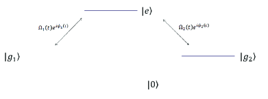
Figure 2.2.1.  State-transfer diagram

Schematic representation of the state-transfer protocol described by the Hamiltonian of Eq. (LABEL:eq:2.2.9). The two ground states $\left.|g_{1}\right\rangle$ and $\left.|g_{2}\right\rangle$ are coupled to the excited state $\left.|e\right\rangle$ via two time-dependent classical laser fields. The spectator state $\left.|0\right\rangle$ does not couple to any other state (which is why we call it a spectator state).