Robust Block Coordinate Descent
May 8, 2015

Abstract

In this paper we present a novel randomized block coordinate descent method for the minimization of a convex composite objective function. The method uses (approximate) partial second-order (curvature) information, so that the algorithm performance is more robust when applied to highly nonseparable or ill conditioned problems. We call the method Robust Coordinate Descent (RCD). At each iteration of RCD, a block of coordinates is sampled randomly, a quadratic model is formed about that block and the model is minimized approximately/inexactly to determine the search direction. An inexpensive line search is then employed to ensure a monotonic decrease in the objective function and acceptance of large step sizes. We prove global convergence of the RCD algorithm, and we also present several results on the local convergence of RCD for strongly convex functions. Finally, we present numerical results on large-scale problems to demonstrate the practical performance of the method.

1 Introduction

In this work we are interested in solving the following convex composite optimization problem

(1) $$\min_{x\in\mathbb{R}^{N}}F(x):=f(x)+\Psi(x),$$

where $f(x)$ is a smooth convex function and $\Psi(x)$ is a (possibly) nonsmooth, block separable, extended real valued convex function (this will be defined precisely in Section 2.5). Problems of the form of (1) arise in many important scientific fields, and applications include machine learning [29], regression [27] and compressed sensing [4, 3, 5]. Often the term $f(x)$ is a data fidelity term, and the term $\Psi(x)$ represents some kind of regularization.

Frequently, problems of the form of (1) are large-scale problems, i.e., the size of $N$ is of the order of a million or a billion. Large-scale problems impose restrictions on the types of methods that can be employed for the solution of (1). In particular, the methods should have low per iteration computational cost, otherwise completing even a single iteration of the method might require unreasonable time. The methods must also rely only on simple operations such as inner products or matrix vector products, and ideally, they should offer fast progress towards optimality.

First order methods, and in particular randomized coordinate descent methods, have found great success in this area because they can take advantage of the underlying problem structure (separability and block structure), and satisfy the requirements of low computational cost and low storage requirements. For example, in [20] the authors show that their randomized coordinate descent method was able to solve sparse problems with millions of variables in a reasonable amount of time.

Unfortunately, randomized coordinate descent methods have two significant drawbacks. First, due to its coordinate nature, it is efficient only on problems with high degree of separability, and performance suffers when there is a high dependency between variables. Second, as a first-order method, coordinate descent methods do not usually capture essential curvature information of the problem and have been shown to struggle on complicated sparse problems [8].

The purpose of this work is to overcome these drawbacks by equipping a randomized block coordinate descent method with approximate partial second-order information. In particular, at every iteration of RCD the direction is obtained by solving approximately a block piece-wise quadratic model, where the model includes a matrix representing approximate second order information. Then, a line search is employed in order to guarantee a monotonic decrease of the objective function.

RCD randomly selects a block of coordinates at every iteration, which is inexpensive. Although the per iteration computational cost of the method may be higher than other randomized coordinate descent methods, we show that in practise the method is more robust and the total number of iterations decreases. In particular we show that RCD is able to solve difficult problems, on which other coordinate descent method may struggle. RCD uses an inexact search direction, (the termination condition for the block piecewise quadratic subproblem is inspired by [2]), coupled with a line search to ensure a monotonic decrease in the function values, and we prove global convergence of RCD and study its local convergence properties.

1.1 Literature review

Coordinate descent methods are some of the oldest iterative methods, and they are often better known in the literature under various names such as Jacobi methods, Gauss-Seidel methods, among others. It has been observed that these methods suffer from poor practical performance, particularly on ill-conditioned problems. However, as we enter the era of big data, coordinate descent methods are coming back into favour, because of their ability to provide approximate solutions of some realistic very large/huge scale problems in a reasonable amount of time.

Currently, randomized coordinate descent methods include that of Richtàrik and Takàč [20], where the method can be applied to unconstrained convex composite optimization problems of the form (1). The algorithm is supported by theoretical convergence guarantees in the form of high probability iteration complexity results, and [20] also reports very impressive practical performance on highly separable large scale problems. The work has also been extended to the parallel case [21], to include acceleration techniques [7], and to include the use of inexact updates [26].

Other important works on randomized coordinate descent methods include methods for huge-scale problems [16], work in [13] that improves the complexity analysis of [21], coordinate descent methods for group lasso [19, 25] and general regularizers [24, 28] and coordinate descent for constrained optimization problems [14].

Unfortunately, on ill-conditioned problems, or problems that are highly nonseparable, first order methods can display very poor practical performance, and this has prompted the study of methods that employ second order information. To this end, recently there has been a flurry of research on Newton-type methods for problems of the general form (1), or a special case where $\Psi(x)=\|x\|_{1}$. For example, Karimi and Vavasis [10] have developed a proximal quasi-Newton method for $l_{1}$-regularized least squares problems, Lee, Sun and Saunders [11, 12] have proposed a family of Newton-type methods for solving problems of the form (1) and Scheinberg and Tang [23] present iteration complexity results for a proximal Newton-type method. Moreover, the authors in [2] extended standard inexact Newton-type methods to the case of minimization of a composite objective involving a smooth convex term plus an $l_{1}$-regularizer term. Finally, there exists parallel deterministic [6] and sequential active set [22] block coordinate descent methods, where the authors incorporate some block second-order information in the algorithmic process.

We believe that the works in [2, 6] can lead the way to allow general randomized coordinate descent to practically incorporate second-order information and in this paper we propose a method which combines the ideas in [2, 6, 20].

1.2 Core ideas and Major Contributions

In this section we list several of the core ideas and major contributions of this work on randomized block coordinate descent methods. The first two points briefly describe the idea of incorporating (approximate) partial second-order (curvature) information (which have been also presented in a similar way in [6]), whilst the last three are contributions of this paper.

1. Incorporation of some second order information. RCD uses a quadratic model to determine the search direction, which incorporates a user defined positive definite matrix $H^{(i)}(x_{k})$. If $H^{(i)}(x_{k})$ approximates the Hessian, then second order information is incorporated into the quadratic model, and the search direction obtained by minimizing the model is an approximate Newton-type direction. We stress that $H^{(i)}(x)$ can change at every iteration and this is an advantage over the method in [20] where the matrix is fixed at the start of the algorithm for each block of coordinates.

2. Inexact updates. To ensure that this method is computationally practical, it is imperative that the iterates are inexpensive, and RCD achieves this through the use of inexact updates. Any algorithm can be used to approximately minimize the quadratic model. Moreover, the stopping conditions for inner solve are easy to verify; they depend upon quantities that are easy/inexpensive to obtain, or may be available as a byproduct of the inner search direction solver.

3. Blocks can vary throughout iterations. If $\Psi(x)$ is completely separable into coordinates then we do not restrict ourselves to a fixed block structure; rather we allow the blocks of coordinates to change at any iteration. This is important because every element of the Hessian can be accessed (this is discussed further in Section 3.2.2).

4. Line search. The algorithm includes a line search step to ensure a monotonic decrease of the objective function as iterates progress. The line search is inexpensive to perform because, at each iteration, it depends on a single block of coordinates only. One of the major advantages of incorporating second-order information combined with line search is to allow in practice the selection of large step sizes (close to one). This is because unit step sizes can substantially improve the practical efficiency of a method. We prove that if $f$ is strongly convex, then close to the optimal solution unit step sizes are selected. In fact, for all experiments that we performed, unit step sizes were accepted by line search for the majority of the iterations.

5. Convergence theory. We provide global convergence results to show that the RCD algorithm is guaranteed to converge in the limit. We also provide local convergence theory for strongly convex functions $f$. In particular, depending on the choice of stopping condition for the inner search direction solve and the matrix $H^{(i)}(x_{k})$, we show that close to the optimal solution RCD has on expectation block quadratic or superlinear rate of convergence.

1.3 Format of the paper

The paper is organised as follows. In Section 2 we introduce the notation and definitions that are used throughout this paper, as well as giving several technical results. We also define the quadratic model that is used in the algorithm, prove the equivalence of some stationarity conditions for problem (1), and define a continuous measure of the distance of the current point from the set of solutions of (1). A thorough description of the RCD algorithm is presented in Section 3, including how the blocks are selected/sampled at each iteration, a description of the search direction and line search, several suggestions for the matrices $H^{(i)}(x_{k})$, and we also present several concrete examples.

The second half of the paper is devoted to providing convergence results and numerical experiments. In Sections 4, global convergence results are presented, which do not require $f$ to be convex. Local convergence theory for RCD is presented in Section 5. There we show that, close to optimality line search accepts unit step sizes. Moreover, if both the stopping conditions for the inner search direction solve and the matrix $H^{(i)}(x_{k})$ are chosen appropriately, then RCD has on expectation block quadratic or superlinear rate of convergence. Finally, several numerical experiments are presented in Section 6, which show that the algorithm performs very well in practice.

2 Preliminaries

In this section we introduce the notation and definitions that are used in this paper, and we also present some important technical results. Throughout the paper $\|\cdot\|\equiv\sqrt{\langle\cdot,\cdot\rangle}$ and $\|\cdot\|_{A}\equiv\sqrt{\langle\cdot,A\cdot\rangle}$, where $A$ is a positive definite matrix. Moreover, $\lambda_{\min}(\cdot)$ and $\lambda_{\max}(\cdot)$ denote the smallest and largest eigenvalue of $\cdot$, respectively.

2.1 Subgradient and subdifferential

For a function $\Phi:\mathbb{R}^{N}\to\mathbb{R}\cup\{+\infty\}$ the elements $s\in\mathbb{R}^{N}$ that satisfy

$$\Phi(y)\geq\Phi(x)+\langle s,y-x\rangle,$$

are called the subgradients of $\Phi$ at point $x$. In words, all elements defining a linear function that supports the function $\Phi$ at point $x$ are subgradients. The set of all $s$ at a point $x$ is called the subdifferential of $\Phi$ and it is denoted by $\partial\Phi(x)$.

2.2 Convexity

A function $\Phi:\mathbb{R}^{N}\to\mathbb{R}\cup\{+\infty\}$ is strongly convex with convexity parameter $\mu_{\Phi}>0$ if for all $x,y\in\mathbb{R}^{N}$, and where $s\in\partial\Phi(x)$,

$$\Phi(y)\geq\Phi(x)+\langle s,y-x\rangle+\tfrac{\mu_{\Phi}}{2}\|y-x\|^{2}.$$

If $\mu_{\Phi}=0$. then function $\Phi$ is said to be convex.

2.3 Convex conjugate and proximal mapping

For a convex function $\Phi:\mathbb{R}^{N}\to\mathbb{R}\cup\{+\infty\}$, its convex conjugate is defined as $\Phi^{*}(y)\equiv:=\sup_{u\in\mathbb{R}^{N}}\langle u,y\rangle-\Phi(u).$ The proximal mapping of a convex function $\Psi$ at $x$ is

(2) $${\rm{prox}}_{\Psi}(x):=\arg\min_{y\in\mathbb{R}^{N}}\Psi(y)+\frac{1}{2}\|y-x\|^{2},$$

and the proximal mapping of its convex conjugate $\Psi^{*}$ is

(3) $${\rm{prox}}_{\Psi^{*}}(x):=\arg\min_{y\in\mathbb{R}^{N}}\Psi^{*}(y)+\frac{1}{2}\|y-x\|^{2}.$$

The following relation holds between the two proximal mappings.

Lemma 1 (Chapter 1, ($1.4$) in [1]).

Let $\Psi$ be a convex function and let $\Psi^{*}$ denote its convex conjugate. Then, $x={\rm{prox}}_{\Psi}(x)+{\rm{prox}}_{\Psi^{*}}(x)$ for all $x$.

From Chapter $1$ of [1], we also see that ${\rm{prox}}_{\Psi}(\cdot)$ and ${\rm{prox}}_{\Psi^{*}}(\cdot)$ are nonexpansive

(4) $$\|{\rm{prox}}_{\Psi}(y)-{\rm{prox}}_{\Psi}(x)\|\leq\|y-x\|,\quad\mbox{and}\quad\|{\rm{prox}}_{\Psi^{*}}(y)-{\rm{prox}}_{\Psi^{*}}(x)\|\leq\|y-x\|.$$

Finally, from Chapter $1$ of [1] we have

(5) $${\rm{prox}}_{\Psi^{*}}(x)\in\partial\Psi({\rm{prox}}_{\Psi}(x)).$$

2.4 Block decomposition of $\mathbb{R}^{N}$

Let $U\in\mathbb{R}^{N\times N}$ be a column permutation of the $N\times N$ identity matrix and further let $U=[U_{1},U_{2},\dots,U_{n}]$ be a decomposition of $U$ into $n$ submatrices, where $U_{i}$ is $N\times N_{i}$ and $\sum_{i=1}^{n}N_{i}=N$. It is clear that any vector $x\in\mathbb{R}^{N}$ can be written uniquely as $x=\sum_{i=1}^{n}U_{i}x^{(i)},$ where $x^{(i)}\in\mathbb{R}^{N_{i}}$ and block $i$ denotes a subset of $\{1,2,\dots,N\}$. Moreover, these vectors are given by

(6) $$x^{(i)}:=U_{i}^{T}x.$$

2.5 Block decomposition of $\Psi$

The function $\Psi:\mathbb{R}^{N}\to\mathbb{R}\cup\{+\infty\}$ is assumed to be block separable. That is, we assume that $\Psi(x)$ can be decomposed as:

(7) $$\Psi(x)=\sum_{i=1}^{n}\Psi_{i}(x^{(i)}),$$

where the functions $\Psi_{i}:\mathbb{R}^{N_{i}}\to\mathbb{R}\cup\{+\infty\}$ are convex.

Notice that if $n=N$, $\Psi(x)$ is said to be separable (into coordinates), whereas if $n<N$, then $\Psi(x)$ is said to be block separable (separable into blocks of coordinates).

The following relationship will be used repeatedly in this work:

(8) $$\Psi(x+U_{i}t^{(i)})-\Psi(x) = \Big{(}\sum_{j\neq i}\Psi_{j}(x^{(j)})+\Psi_{i}(x^{(i)}+t^{(i)})\Big{)}-\Big{(}\sum_{j\neq i}\Psi_{j}(x^{(j)})+\Psi_{i}(x^{(i)})\Big{)}$$

$$= \Psi_{i}(x^{(i)}+t^{(i)})-\Psi_{i}(x^{(i)}).$$

2.6 Block Lipschitz continuity of $f$

Throughout the paper we assume that the gradient of $f$ is block Lipschitz, uniformly in $x$. This means that, for all $x\in\mathbb{R}^{N}$, $i\subseteq\{1,2,\dots,n\}$ and $t^{(i)}\in\mathbb{R}^{N_{i}}$ we have

(9) $$\|\nabla_{i}f(x+U_{i}t^{(i)})-\nabla_{i}f(x)\|\leq L_{i}\|t^{(i)}\|,$$

where $\nabla_{i}f(x)\overset{\eqref{U_i}}{=}U_{i}^{T}\nabla f(x)$. An important consequence of (9) is the following standard inequality [15, p.57]:

(10) $$f(x+U_{i}t^{(i)})\leq f(x)+\langle\nabla_{i}f(x),t^{(i)}\rangle+\tfrac{L_{i}}{2}\|t^{(i)}\|^{2}.$$

2.7 Piecewise Quadratic Model

For fixed $x\in\mathbb{R}^{N}$, we define a piecewise quadratic approximation of $F$ around the point $(x+t)\,\in\mathbb{R}^{N}$ as follows:

(11) $$F(x+t)\approx Q(x;t):=f(x)+\sum_{i=1}^{n}Q_{i}(x,t^{(i)}),$$

where

(12) $$Q_{i}(x,t^{(i)}):=\langle\nabla_{i}f(x),t^{(i)}\rangle+\frac{1}{2}\|t^{(i)}\|_{H^{(i)}(x)}^{2}+\Psi_{i}(x^{(i)}+t^{(i)}),$$

and $H^{(i)}(x)\in\mathbb{R}^{N_{i}\times N_{i}}$ is any positive definite matrix, which possibly depends on $x$. Notice that $Q(x;0)=F(x)$ and that $Q_{i}(x,t^{(i)})$ is the quadratic model for block $i$.

2.8 Stationarity conditions

The following theorem gives the equivalence of some stationarity conditions of problem (1).

Theorem 2.

The following are equivalent first order optimality conditions of problem (1).

1. $\nabla f(x)+s=0$ and $s\in\partial\Psi(x)$,

2. $-\nabla f(x)\in\partial\Psi(x)$,

3. $\nabla f(x)+\frac{1}{\beta}{\rm{prox}}_{(\beta\Psi)^{*}}\left(x-\beta\nabla f(x)\right)=0$,

4. $x={\rm{prox}}_{\beta\Psi}\left(x-\beta\nabla f(x)\right)$,

where $\beta$ is any positive constant.

Proof.

It is easy to see that $(i)$ are first-order optimality conditions of problem (1), which can be obtained by using the definition of subgradient. It is trivial to show that $(i)\Longleftrightarrow(ii)$. By Lemma 1, we have that $(iii)\Longleftrightarrow(iv)$. We now show that $(iii)\Longleftrightarrow(ii)$. We rewrite $(ii)$ as

$$0\in\beta\nabla f(x)+y-x+\beta\partial\Psi(x)\quad\mbox{and}\quad y=x,$$

which is satisfied if and only if $(iv)$ holds, hence, if and only if $(iii)$ holds. ∎

Let us define the continuous function

(13) $$g(x;t):=\nabla f(x)+H(x)t+\frac{1}{\beta}{\rm{prox}}_{(\beta\Psi)^{*}}\big{(}x+t-\beta(\nabla f(x)+H(x)t)\big{)},$$

where $\beta$ is a positive constant, which is used in the local convergence analysis (Section 5). By Theorem 2, the points that satisfy $g(x;0)=\nabla f(x)+\frac{1}{\beta}{\rm{prox}}_{(\beta\Psi)^{*}}\left(x-\beta\nabla f(x)\right)=0$ are stationary points for problem (1). Hence, $g(x;0)$ is a continuous measure of the distance from the set of stationary points of problem (1).

Furthermore, let us define

$$g_{i}(x;t^{(i)}) := \nabla_{i}f(x)+H^{(i)}(x)t^{(i)}$$

$$+\frac{1}{\beta}{\rm{prox}}_{(\beta\Psi)^{*}_{i}}\big{(}x^{(i)}+t^{(i)}-\beta(\nabla_{i}f(x)+H^{(i)}(x)t^{(i)})\big{)},$$

which will be used as a continuous measure for the distance from stationarity of the block piecewise quadratic function $Q_{i}(x_{k};t^{(i)})$.

3 The Algorithm

In this section we present the Robust Coordinate Descent (RCD) algorithm for solving problems of the form (1). There are three key steps in the algorithm: (step $4$) the coordinates are sampled randomly; (step $5$) the quadratic model (12) is solved approximately until the stopping conditions (16) are satisfied to give a search direction; (step $6$) a line search is performed to find a step size that ensures a sufficient reduction in the objective value. Once these key steps have been performed, the current point $x_{k}$ is updated to give a new point $x_{k+1}$, and the process is repeated.

The following assumption is used in RCD. The reason this assumption is used will be made clear in Section 3.1.

Assumption 3.

The block decomposition of $\mathbb{R}^{N}$ used within RCD, and the associated probability distribution, adhere to the block structure of $\Psi(x)$.

We now present pseudocode for the algorithm, while a thorough description of each of the key steps in the algorithm will follow in the rest of this section.

1:  Input Choose $x_{0}\in\mathbb{R}^{N}$, $\theta\in(0,1/2)$ and $\beta>0$.

2:  Initialize a decomposition of $\mathbb{R}^{N}$ and a probability distribution following Assumption 3

3:  for $k=1,2,\cdots$ do

4:     Sample a block of coordinates $i$ with probability $p_{i}>0$.

5:     If $g_{i}(x_{k};0)=0$ then go to Step $3$; else approximately solve

(15) $$t_{k}^{(i)}:=\operatorname*{arg\,min}_{t^{(i)}}Q_{i}(x_{k};t^{(i)}),$$

until the stopping conditions

(16) $$Q(x_{k};U_{i}t^{(i)}_{k})<Q(x_{k};0)\quad\mbox{and}\quad\|g_{i}(x_{k};t^{(i)}_{k})\|\leq\eta_{k}^{i}\|g_{i}(x_{k};0)\|,$$

are satisfied, (where $\eta_{k}^{i}\in[0,1)$).

6:     Perform a backtracking line search along the direction $t_{k}^{(i)}$ starting from $\alpha=1$. That is, find $\alpha\in(0,1]$ such that

(17) $$F(x_{k})-F(x_{k}+\alpha U_{i}t_{k}^{(i)})\geq\theta\left(\ell(x_{k};0)-\ell(x_{k};\alpha U_{i}t_{k}^{(i)})\right),$$

where

(18) $$\ell(x_{k};t):=f(x_{k})+\langle\nabla f(x_{k}),t\rangle+\Psi(x_{k}+t).$$

7:     Update $x_{k+1}=x_{k}+\alpha U_{i}t_{k}^{(i)}$

8:  end for

Algorithm 1 Robust Coordinate Descent (RCD)

3.1 Block structure and selection of coordinates (Steps $\boldsymbol{2}$ & $\boldsymbol{4}$)

One of the crucial ideas of this algorithm is that the block of coordinates to be updated at each iteration is chosen randomly. This allows the coordinates to be selected very quickly. In this section we explain in detail, how the blocks are selected/sampled at each iteration. We also give examples of how coordinates can be randomly sampled such that Assumption 3 is satisfied.

3.1.1 $\Psi$ is block separable with $n<N$

When $\Psi$ has a fixed block structure (i.e., $n<N$), the block decomposition of $\mathbb{R}^{N}$ (via the matrix $U=[U_{1},\dots,U_{n}]$) described in Section 2.4 is fixed at the start of the algorithm to coincide with the block structure of $\Psi$, and does not change as iterations progress. There are several ways to initialize a sampling scheme to use in RCD that follow Assumption 3.

1. Fix the $n$ blocks of coordinates according to the decomposition of $\mathbb{R}^{N}$ defined by $U$, and in the algorithm, select each block of coordinates with some probability $p_{i}$. (e.g., uniform probabilities $p_{i}=1/n>0$ for all $i=1,\dots,n$).

2. Perform (single) coordinate descent, where at each iteration of RCD, the coordinate $i$ is selected with some probability $p_{i}$ (e.g., uniform probabilities $p_{i}=1/N$ for all $i$).

3. Perform block coordinate descent, where each block of coordinates has cardinality $N_{\min}:=\min\{N_{1},\dots,N_{n}\}$. The restriction is that, at any iteration $k$, the sampled coordinates forming block $i$, must all belong to the same block of $N_{j}$ coordinates defined by submatrix $U_{j}$. (i.e., Assumption 3 is satisfied because the decomposition of $U$ is obeyed.) Recall that $\Psi$ is separable into $n$ blocks. Let the total number of subblocks be $l(>n)$, where we assume that each coordinate $1,\dots,N$ appears in at least one of the $l$ blocks. Then each subblock is selected with probability $p_{i}$.

3.1.2 $\Psi$ is separable with $n=N$

When $\Psi$ is separable into coordinates, we have complete control over the indices that are updated at each iteration.

Let $\tau$ denote the block size (number of coordinates that are updated at any iteration $k$), where $1\leq\tau\leq N$. Note that there are ${}^{N}C_{\tau}$ subsets of $\tau$ coordinates that can be made from the set $\{1,\dots,N\}$. At any iteration $k$ of RCD, a subset of coordinates $i_{k}$ with $|i_{k}|=\tau$ is sampled with some probability $p_{i}$ (e.g., uniform probabilities $p_{i}=1/^{N}C_{\tau}>0$ for all $i$). Note that in practice, one never explicitly forms the ${}^{N}C_{\tau}$ different blocks in order to randomly pick one with some probability $p_{i}$. Instead, $\tau$ coordinates are sampled randomly without replacement.

3.2 The search direction and Hessian approximation (Step $\boldsymbol{5}$)

In this section we describe how RCD determines the search direction. In particular, RCD forms a quadratic model for block $i$, and minimizes the model approximately until the stopping conditions (16) are satisfied, giving an ‘inexact’ search direction.

We also describe the importance of the choice of matrix $H$, which is an approximate second order information term. From now on, we will often use the shorthand $H_{k}^{(i)}\equiv H^{(i)}(x_{k})$.

3.2.1 The search direction

At each iteration the update/search direction is found as follows. The subproblem (15), (where $Q_{i}(x_{k};t^{(i)})$ is defined in (12)) is approximately solved, and the search direction $t_{k}^{(i)}$ is accepted when the stopping conditions (16) are satisfied, for some $\eta_{k}^{i}\in[0,1)$. Notice that

(19) $$Q(x;U_{i}t^{(i)})-Q(x;0) \overset{\eqref{Def_Q}}{=} \langle\nabla_{i}f(x),t^{(i)}\rangle+\frac{1}{2}\|t^{(i)}\|_{H^{(i)}}^{2}+\Psi(x+U_{i}t^{(i)})-\Psi(x)$$

$$\overset{\eqref{Eq_PsivsPsii}}{=} \langle\nabla_{i}f(x),t^{(i)}\rangle+\frac{1}{2}\|t^{(i)}\|_{H^{(i)}}^{2}+\Psi_{i}(x^{(i)}+t^{(i)})-\Psi_{i}(x^{(i)}).$$

Hence, from (19), the stopping conditions (16) depend on block $i$ only, and are therefore inexpensive to verify, meaning that they are implementable.

Remark 4.

• At some iteration $k$, it is possible that $g_{i}(x_{k};0)=0$. In this case, it is easy to verify that the optimal solution of subproblem (15) is $t^{(i)}_{k}=0$. Therefore, before calculating $t^{(i)}_{k}$ we check a-priori if condition $g_{i}(x_{k};0)=0$ is satisfied.

• Notice that, unless at optimality (i.e., $g(x_{k};0)=0$), there will always be blocks $i$ such that $g_{i}(x_{k};0)\neq 0$, which implies that $t^{(i)}_{k}\neq 0$. Hence, RCD will not stagnate.

• Following similar arguments as those made in [2, p.4], we prove this in Lemma 8 that both conditions are required to ensure that $t_{k}^{(i)}$ is a descent direction.

3.2.2 The Hessian approximation

Arguably, them most important feature of this method is that the quadratic model (12) incorporates second order information in the form of a positive definite matrix $H_{k}^{(i)}$. This is key because, depending upon the choice of $H_{k}^{(i)}$, it makes the method robust. Moreover, at each iteration, the user has complete freedom over the choice of $H_{k}^{(i)}\succ 0$.

We now provide a few suggestions for the choice of $H_{k}^{(i)}$. (This list is not intended to be exhaustive.) Notice that in each case there is a trade off between a matrix that is inexpensive to work with, and one that is a more accurate representation of the true block Hessian.

1. Clearly, the simplest option is to set $H_{k}^{(i)}=I$ for all $i$ and $k$. In this case no second order information is employed by the method.

2. A second option is to let $H_{k}^{(i)}=\text{diag}(\nabla_{i}^{2}f(x_{k}))$. In this case $H_{k}^{(i)}$ and it’s inverse are inexpensive to work with. Moreover, if $f$ is quadratic, then $\nabla^{2}f(x_{k})$ is constant for all $k$, so $H=\text{diag}(\nabla^{2}f(x))$ can be computed and stored at the start of the algorithm and elements can be accessed throughout the algorithm as necessary. This is very effective if $\text{diag}(\nabla^{2}f(x))$ is a good approximation to $\nabla^{2}f(x)$.

3. A third option is to let $H_{k}^{(i)}=\nabla_{i}^{2}f(x_{k})$ (i.e., $H_{k}^{(i)}$ is a principal minor of the Hessian). In this case, $H_{k}^{(i)}$ provides the most accurate second order information, but it is (potentially) more computationally expensive to work with. In practice the matrix $\nabla_{i}^{2}f(x_{k})$ is used in a matrix-free way and is not explicitly stored. For example, there may be an analytic formula for performing matrix-vector products with $\nabla_{i}^{2}f(x_{k})$, or techniques from automatic differentiation could be employed, see [18, Section $7$].

4. Another option is to use a quasi-Newton type approach where $H_{k}^{(i)}$ is an approximation to $\nabla_{i}^{2}f(x_{k})$ based on the limited-memory BFGS update scheme, see [18, Section $8$]. This approach might be more suitable in cases that the problem is not very ill-conditioned and additionally performing matrix-vector products with $\nabla_{i}^{2}f(x_{k})$ is expensive.

Remark 5.

If any of the matrices above are not positive definite, then they can be altered to make them so. For example, if $H_{k}^{(i)}$ is diagonal, any zero that appears on the diagonal can be replaced with a positive number. Moreover, if $\nabla_{i}^{2}f(x_{k})$ is not positive definite, a multiple of the identity can be added to it.

An advantage of the RCD algorithm (if Option 3 is used for $H_{k}^{(i)}$) is that all elements of the Hessian can be accessed. This is because the blocks of coordinates can change at every iteration, and so too can matrix $H_{k}^{(i)}$. This makes RCD extremely flexible and is particularly advantageous when there are large off diagonal elements in the Hessian.

3.3 The line search (Step $\boldsymbol{6}$)

The stopping conditions (16) ensure that $t_{k}^{(i)}$ is a descent direction, but if the full step $x_{k}+U_{i}t_{k}^{(i)}$ is taken, a reduction in the function value (1) is not guaranteed. To this end, we include a line search step in our algorithm in order to guarantee monotonic decrease of function $F$. Essentially, the line search guarantees the sufficient decrease of $F$ at every iteration, where sufficient decrease is measured by the loss function (18).

In particular, for fixed $\theta\in(0,1/2)$, we require that for some $\alpha\in(0,1]$, (17) is satisfied. (In Lemma 8 we prove that there exists a subinterval $(0,\tilde{\alpha}]$ of $(0,1]$ in which (17) is satisfied.) Notice that

(20) $$\ell(x;U_{i}t^{(i)})-\ell(x;0) \overset{\eqref{Def_lossfunctionli}}{=} \langle\nabla_{i}f(x),t^{(i)}\rangle+\Psi(x+U_{i}t^{(i)})-\Psi(x)$$

$$\overset{\eqref{Eq_PsivsPsii}}{=} \langle\nabla_{i}f(x),t^{(i)}\rangle+\Psi_{i}(x^{(i)}+t^{(i)})-\Psi_{i}(x^{(i)}),$$

which shows that the calculation of the right hand side of (17) only depends upon block $i$, so it is inexpensive. Moreover, the line search condition (Step 5) involves the difference between function values $F(x_{k})-F(x_{k}+\alpha U_{i}t_{k}^{(i)})$. Fortunately, while function values can be expensive to compute, the difference in the objective value between iterates need not be (this is discussed in more detail in Section 3.4).

3.4 Examples

In this section we provide several examples to demonstrate the practicality of the algorithm. These examples demonstrate that the difference of function values $F(x_{k})-F(x_{k}+\alpha U_{i}t_{k}^{(i)})$ required by the line search conditions (17), can be easy/inexpensive to implement and verify.

3.4.1 Quadratic loss plus regularization example

Suppose that $f(x)=\tfrac{1}{2}\|Ax-b\|^{2}$ and $\Psi(x)\neq 0,$ where $A\in\mathbb{R}^{m\times N}$, $b\in\mathbb{R}^{m}$ and $x\in\mathbb{R}^{N}$. Then

$$F(x_{k})-F(x_{k}+\alpha U_{i}t_{k}^{(i)}) \overset{\eqref{Eq_PsivsPsii}}{=} f(x_{k})+\Psi_{i}(x^{(i)})$$

$$-f(x_{k}+\alpha U_{i}t_{k}^{(i)})-\Psi_{i}(x_{k}^{(i)}+\alpha t_{k}^{(i)})$$

$$= \Psi_{i}(x^{(i)})-\alpha\langle\nabla_{i}f(x),t_{k}^{(i)}\rangle-\frac{\alpha^{2}}{2}\|A_{i}t_{k}^{(i)}\|_{2}^{2}$$

$$-\Psi_{i}(x_{k}^{(i)}+\alpha t_{k}^{(i)}).$$

Notice that calculation of $F(x_{k})-F(x_{k}+\alpha U_{i}t_{k}^{(i)})$ as a function of $\alpha$ only depends on block $i$, hence, it is inexpensive. Moreover, in some cases some of the quantities in (3.4.1) are already needed in the computation of the search direction $t$, so regarding the line search step, they essentially come “for free”.

3.4.2 Logistic regression example

Suppose that

$$f(x)\equiv\sum_{j=1}^{m}\log(1+e^{-b_{j}a_{j}^{T}x})\quad\mbox{and}\quad\Psi(x)\neq 0,$$

where $a_{j}^{T}$ is the $j$th row of a matrix $A\in\mathbb{R}^{m\times n}$ and $b_{j}$ is the $j$th component of vector $b\in\mathbb{R}^{m}$. As before, we need to evaluate (3.4.1). Let us split calculation of $F(x_{k})-F(x_{k}+\alpha U_{i}t_{k}^{(i)})$ in parts. The first part $\Psi_{i}(x^{(i)})-\Psi_{i}(x_{k}^{(i)}+\alpha t_{k}^{(i)})$ is inexpensive, since it depends only on block $i$. The second part $f(x_{k})-f(x_{k}+\alpha U_{i}t_{k}^{(i)})$ is more expensive because is depends upon the logarithm. In this case, one can calculate $f(x_{0})$ once at the beginning of the algorithm and then update $f(x_{k}+\alpha U_{i}t_{k}^{(i)})$ $\forall k\geq 1$ less expensively. In particular, let us assume that the following terms:

(22) $$e^{-b_{j}a_{j}^{T}x_{0}}\quad\forall j\quad\mbox{and}\quad f(x_{0})=\sum_{j=1}^{m}\log(1+e^{-b_{j}a_{j}^{T}x_{0}}),$$

are calculated once and stored in memory. Then, at iteration $1$, the calculation of $f(x_{0}+\alpha U_{i}t^{(i)}_{0})=\sum_{j=1}^{m}\log(1+e^{-b_{j}a_{j}^{T}x_{0}}e^{-\alpha b_{j}a_{j}^{T}(U_{i}t^{(i)}_{0})})$ is required for different values of $\alpha$ by the backtracking line search algorithm. The most demanding task in calculating $f(x_{0}+\alpha U_{i}t^{(i)}_{0})$ is the calculation of the products $b_{j}a_{j}^{T}(U_{i}t^{(i)}_{0})$ $\forall j$ once, which is inexpensive since $\forall j$ this operation depends only on block $i$. Having $b_{j}a_{j}^{T}(U_{i}t^{(i)}_{0})$ $\forall j$ and (22) calculation of $f(x_{0})-f(x_{0}+\alpha U_{i}t^{(i)}_{0})$ for different values of $\alpha$ is inexpensive. At the end of the process, $f(x_{1})$ and $e^{-b_{j}a_{j}^{T}x_{1}}$ $\forall j$ will be given for free, and the same process can be followed for the calculation of $f(x_{1})-f(x_{1}+\alpha U_{i}t^{(i)}_{1})$ etc.

4 Global convergence theory without convexity of $f$

In this section we provide global convergence theory for the RCD algorithm. Note that we do not assume that $f$ is convex. Throughout this section we denote $H^{(i)}_{k}\equiv H^{(i)}(x_{k})$. The following assumptions are made about $H_{k}^{(i)}$ and $f$.

Assumption 6.

There exist constants $0<\lambda_{i}\leq\Lambda_{i}$, such that the sequence $\{H_{k}^{(i)}\}_{k\geq 0}$ satisfies

(23) $$0<\lambda_{i}\leq\lambda_{\min}(H_{k}^{(i)})\quad\text{and}\quad\lambda_{\max}(H_{k}^{(i)})\leq\Lambda_{i},\quad\text{for all }i\text{ and }k.$$

Assumption 7.

The function $f$ is smooth, bounded below, and satisfies (9) for all $i$.

Assumption 6 explains that the Hessian approximation $H_{k}^{(i)}$ must be positive definite for all blocks $i$ at all iterations $k$. Assumption 7 explains that $f$ must be block Lipschitz for all blocks $i$ and all iterations $k$.

Before proving global convergence of RCD, we present several technical results. The following lemma shows that if $t^{(i)}_{k}$ is nonzero, then $F$ is decreased.

Lemma 8.

Let Assumptions 6 and 7 hold. Let $\theta\in(0,1/2)$ and let $x_{k}$ and $i$ be generated by RCD. Then Step 6 of RCD will accept a step-size $\alpha$ that satisfies

(24) $$\alpha\geq\tilde{\alpha}\qquad\text{where}\qquad\tilde{\alpha}:=(1-\theta)\frac{\lambda_{i}}{2L_{i}}.$$

Furthermore,

(25) $$F(x_{k})-F(x_{k}+\alpha U_{i}t^{(i)}_{k})>\theta(1-\theta)\frac{\lambda_{i}^{2}}{4L_{i}}\|t^{(i)}_{k}\|^{2}.$$

Proof.

The proof closely follows that of [2, Theorem $3.1$]. From (16),

(26) $$0>Q(x_{k};U_{i}t_{k}^{(i)})-Q(x_{k};0)=\ell(x_{k};U_{i}t_{k}^{(i)})-\ell(x_{k};0)+\frac{1}{2}\|t_{k}^{(i)}\|_{H_{k}^{(i)}}^{2}.$$

Rearranging gives

(27) $$\ell(x_{k};0)-\ell(x_{k};U_{i}t_{k}^{(i)})>\frac{1}{2}\|t_{k}^{(i)}\|_{H_{k}^{(i)}}^{2}\overset{\eqref{Assumption_lambdai}}{\geq}\frac{1}{2}\lambda_{i}\|t_{k}^{(i)}\|^{2}.$$

By Assumption 7, for $\alpha\in(0,1)$, we have

$$F(x_{k}+\alpha U_{i}t_{k}^{(i)})\leq f(x_{k})+\alpha\langle\nabla_{i}f(x),t_{k}^{(i)}\rangle+\frac{L_{i}}{2}\alpha^{2}\|t_{k}^{(i)}\|^{2}+\Psi(x_{k}+\alpha U_{i}t_{k}^{(i)}).$$

Adding $\Psi(x_{k})$ to both sides of the above and rearranging gives

(28) $$F(x_{k})-F(x_{k}+\alpha U_{i}t_{k}^{(i)}) \geq -\alpha\langle\nabla_{i}f(x_{k}),t_{k}^{(i)}\rangle-\frac{L_{i}}{2}\alpha^{2}\|t_{k}^{(i)}\|^{2}$$

$$-\Psi(x_{k}+\alpha U_{i}t_{k}^{(i)})+\Psi(x_{k})$$

$$\overset{\eqref{Eq_differenceloss}}{=} \ell(x_{k};0)-\ell(x_{k};\alpha U_{i}t_{k}^{(i)})-\frac{L_{i}}{2}\alpha^{2}\|t_{k}^{(i)}\|^{2}.$$

By convexity of $\Psi(x)$ we have that

(29) $$\ell(x_{k};0)-\ell(x_{k};\alpha U_{i}t_{k}^{(i)})\geq\alpha(\ell(x_{k};0)-\ell(x_{k};U_{i}t_{k}^{(i)})).$$

Then

$$F(x_{k})-F(x_{k}+\alpha U_{i}t_{k}^{(i)}) - \theta(\ell(x_{k};0)-\ell(x_{k};\alpha U_{i}t_{k}^{(i)}))$$

$$\overset{\eqref{in:3}}{\geq} (1-\theta)\big{(}\ell(x_{k};0)-\ell(x_{k};\alpha U_{i}t^{(i)})\big{)}-\frac{L_{i}}{2}\alpha^{2}\|t_{k}^{(i)}\|^{2}$$

$$\overset{\eqref{Eq_ell_convexity}}{\geq} \alpha(1-\theta)\big{(}\ell(x_{k};0)-\ell_{i}(x_{k};U_{i}t_{k}^{(i)})\big{)}-\frac{L_{i}}{2}\alpha^{2}\|t_{k}^{(i)}\|^{2}$$

$$\stackrel{{\scriptstyle\eqref{in:1}}}{{>}} \frac{1}{2}\big{(}\alpha(1-\theta)\lambda_{i}\|t_{k}^{(i)}\|^{2}-L_{i}\alpha^{2}\|t_{k}^{(i)}\|^{2}\big{)}$$

$$= \frac{\alpha}{2}\big{(}(1-\theta)\lambda_{i}-L_{i}\alpha\big{)}\|t_{k}^{(i)}\|^{2}.$$

From the previous observe that if $\alpha$ satisfies $0\leq\alpha\leq(1-\theta)\frac{\lambda_{i}}{L_{i}}$, then $\alpha$ also satisfies the backtracking line search step of RCD. Suppose that any $\alpha$ that is rejected by the line search is halved for the next line search trial. Then, it is guaranteed that the $\alpha$ that is accepted satisfies (24).

Since the line search condition (17) is guaranteed to be satisfied for some step size $\alpha$, from (17) and convexity of $\ell$ we obtain $F(x_{k})-F(x_{k}+\alpha U_{i}t_{k}^{(i)})\geq\theta\alpha(\ell(x_{k};0)-\ell(x_{k};U_{i}t_{k}^{(i)}))$. Using (27) and (24) in the last inequality we obtain (25). ∎

The following lemma bounds the norm of the direction $t_{k}^{(i)}$ in terms of $g_{i}(x_{k},0)$.

Lemma 9.

Let Assumptions 6 and 7 hold. For $\beta>0$, and $x_{k}$ and $i$ generated by RCD, we have

(30) $$\|t_{k}^{(i)}\|\geq\gamma_{i}\|g_{i}(x_{k};0)\|,\quad\mbox{where}\quad\gamma_{i}:=\frac{1-\eta_{k}^{i}}{\frac{1}{\beta}+2\Lambda_{i}},$$

where $\eta_{k}^{i}$ is defined in (16). Moreover,

(31) $$F(x_{k})-F(x_{k}+{\alpha}U_{i}t_{k}^{(i)})>\theta(1-\theta)\frac{\lambda_{i}^{2}}{4L_{i}}\gamma_{i}^{2}\|g_{i}(x_{k};0)\|^{2}.$$

Proof.

This proof closely follows that of [2, Theorem $3.1$]. Using the reverse triangular inequality and the fact that ${\rm{prox}}_{\Psi^{*}_{i}}(\cdot)$ is nonexpansive, we have that

$$(1-\eta_{k}^{i})\|g_{i}(x_{k};0)\| \stackrel{{\scriptstyle\eqref{Def_stoppingconditions}}}{{\leq}} \|g_{i}(x_{k};0)\|-\|g_{i}(x_{k};t^{(i)}_{k})\|$$

$$\leq \|g_{i}(x_{k};t_{k}^{(i)})-g_{i}(x_{k};0)\|$$

$$\stackrel{{\scriptstyle\eqref{defeq:2}}}{{=}} \|H_{k}^{(i)}t_{k}^{(i)}+\tfrac{1}{\beta}{\rm{prox}}_{(\beta\Psi)^{*}_{i}}\big{(}x_{k}^{(i)}+t_{k}^{(i)}-\beta(\nabla_{i}f(x_{k})+H_{k}^{(i)}t_{k}^{(i)})\big{)}$$

$$-\tfrac{1}{\beta}{\rm{prox}}_{(\beta\Psi)^{*}_{i}}\big{(}x_{k}^{(i)}-\beta\nabla_{i}f(x_{k})\big{)}\|$$

$$\overset{\eqref{Eq_proxnonexpansive}}{\leq} \|H_{k}^{(i)}t_{k}^{(i)}\|+\tfrac{1}{\beta}\|(I-\beta H_{k}^{(i)})t_{k}^{(i)}\|$$

$$\leq (\tfrac{1}{\beta}+2\|H_{k}^{(i)}\|)\|t_{k}^{(i)}\|$$

$$\leq (\tfrac{1}{\beta}+2\Lambda_{i})\|t_{k}^{(i)}\|.$$

Rearranging gives (30), and combining (25) and (30) gives (31).

∎

We now have all the tools to prove global convergence of RCD.

Theorem 10.

Let Assumptions 6 and 7 hold. Then the following hold for RCD:

$$\lim_{k\to\infty}t^{(i)}_{k}=0\quad\forall i\quad\mbox{and}\quad\lim_{k\to\infty}g(x_{k};0)=0.$$

with probability one.

Proof.

By Lemma 8, for $t^{(i)}_{k}\neq 0$ we have that $F(x_{k})>F(x_{k}+{\alpha}U_{i}t^{(i)}_{k})$. Since $F$ is bounded from below and every block $(i)$ has positive probability to be selected, then for $k\to\infty$ the following holds with probability one:

(32) $$\lim_{k\to\infty}F(x_{k})-F(x_{k}+{\alpha}U_{i}t^{(i)}_{k})=0.$$

Using (25) in combination with (32) we get that for $k\to\infty$ with probability one $\|t_{k}^{(i)}\|\to 0$, which proves the first part. Using (30) and $\|t_{k}^{(i)}\|\to 0$ for $k\to\infty$ with probability one we also get that $\|g_{i}(x_{k};0)\|\to 0$ with probability one for $k\to\infty$ Since $g_{i}(x_{k};0)$ is a block of $g(x_{k};0)$, i.e., $g_{i}(x_{k};0)\overset{\eqref{U_i}}{=}U_{i}^{T}g(x_{k};0)$ and since every block $g_{i}(x_{k};0)$ tends to zero as $k\to\infty$ with probability one, then we have that $g(x_{k};0)\to 0$ with probability one. ∎

5 Local convergence theory

In this section we present local convergence theory for RCD. First we discuss some common assumptions that are needed. Throughout the section we set $H_{k}^{(i)}=\nabla_{i}^{2}f(x_{k})$ $\forall i$, where $\nabla_{i}^{2}f(x)$ denotes the principal minor of the Hessian $\nabla^{2}f(x)$ with row (equivalently column) indices in the subset $i$.

Assumption 11.

Function $f$ is strongly convex with strong convexity parameter $\mu_{f}>0$.

By continuity of $f$ we have that $\nabla^{2}f(x)$ is symmetric, and by strong convexity of $f$ we have that $\mu_{f}I\preceq\nabla^{2}f(x)$.

The next theorem explains that, if the Hessian $H\equiv\nabla^{2}f(x)$ is positive definite, then every principal submatrix of it is also positive definite.

Theorem 12 (Theorem 4.3.15 in [9]).

Let $A\in\mathbb{R}^{N\times N}$ be a Hermitian matrix, let $r$ be an integer with $1\leq r\leq N$, and let $A_{r}$ denote any $r\times r$ principal submatrix of $A$ (obtained by deleting $N-r$ rows and the corresponding columns from $A$). For each integer $k$ such that $1\leq k\leq r$ we have $\lambda_{k}(A)\leq\lambda_{k}(A_{r})\leq\lambda_{k+N-r}(A),$ where $\lambda_{k}(\cdot)$ denotes the $k$th eigenvalue of matrix $\cdot$, and the eigenvalues are ordered $\lambda_{1}\leq\dots,\lambda_{N}$.

Corollary 13.

If $f$ is strongly convex with strong convexity parameter $\mu_{f}>0$, then

(33) $$\mu_{f}I\preceq\nabla_{i}^{2}f(x)\qquad\text{for all }i\subseteq\{1,\dots,N\}.$$

Assumption 14.

We assume that the blocks of the Hessian of $f$ are Lipschitz continuous. This means that for all $x\in\mathbb{R}^{N}$, $i\subseteq\{1,2,\dots,n\}$ and $t^{(i)}\in\mathbb{R}^{N_{i}}$ we have

(34) $$\|\nabla_{i}^{2}f(x+U_{i}t^{(i)})-\nabla_{i}^{2}f(x)\|\leq M_{i}\|t^{(i)}\|.$$

The following theorem is used to show that the backtracking line search accepts units step sizes close to optimality for any block $i$. Similarly to [2], in order to prove the previous statement we have to impose sufficient decrease of the quadratic model (15) at every iteration. This means that the inexactness conditions in (16) are replaced by

(35) $$\xi(\ell(x_{k};0)-\ell(x_{k};U_{i}t^{(i)}_{k})) \leq Q(x_{k};0)-Q(x_{k};U_{i}t^{(i)}_{k}),$$

$$\text{and}\;\;\|g_{i}(x_{k};t^{(i)}_{k})\| \leq \eta_{k}^{i}\|g_{i}(x_{k};0)\|,$$

where $\xi\in(\theta,1/2)$ and $\eta_{k}^{i}\in[0,1)$.

Notice that, substituting the equality in (26) into (35), gives

(36) $$\frac{1}{2}\|t^{(i)}_{k}\|_{H^{(i)}_{k}}^{2}\leq(1-\xi)\big{(}\ell(x_{k};0)-\ell(x_{k};U_{i}t^{(i)}_{k})\big{)}.$$

Theorem 15.

Let Assumptions 11 and 14 hold. Let $x_{k}$ and $i$ be generated by RCD. Moreover, let subproblem (15) of RCD be solved inexactly until the inexactness conditions (35) are satisfied. If $\|t^{(i)}_{k}\|\leq 3{\lambda_{i}}(\xi-{\theta})/{M_{i}}$, where $\theta\in(0,1/2)$, $\xi\in(\theta,1/2)$ and $\lambda_{i}\equiv\lambda_{\min}(H_{k}^{(i)})\geq\mu_{f}>0$ $\forall i$ (by Assumption 11), then the backtracking line search step in RCD accepts step sizes $\alpha=1$.

Proof.

The proof closely follows that of [12, Lemma $3.3$]. Using Lipschitz continuity of $H_{k}^{(i)}$ we have that

$$f(x_{k}+U_{i}t^{(i)}_{k})\leq f(x_{k})+\langle\nabla_{i}f(x_{k}),t^{(i)}_{k}\rangle+\tfrac{1}{2}\|t_{k}^{(i)}\|_{H_{k}^{(i)}}^{2}+\tfrac{M_{i}}{6}\|t^{(i)}_{k}\|^{3}.$$

Adding $\Psi(x_{k}+U_{i}t^{(i)}_{k})$ to both sides gives

(37) $$F(x_{k}+U_{i}t^{(i)}_{k}) \leq f(x_{k})+\langle\nabla_{i}f(x_{k}),t^{(i)}_{k}\rangle+\tfrac{1}{2}\|t_{k}^{(i)}\|_{H_{k}^{(i)}}^{2}+\tfrac{M_{i}}{6}\|t^{(i)}_{k}\|^{3}+\Psi(x_{k}+U_{i}t^{(i)}_{k})$$

$$= F(x_{k})+\langle\nabla_{i}f(x_{k}),t^{(i)}_{k}\rangle+\tfrac{1}{2}\|t_{k}^{(i)}\|_{H_{k}^{(i)}}^{2}+\tfrac{M_{i}}{6}\|t^{(i)}_{k}\|^{3}$$

$$+\Psi(x_{k}+U_{i}t^{(i)}_{k})-\Psi(x_{k})$$

$$= F(x_{k})-(\ell(x_{k};0)-\ell(x_{k};U_{i}t^{(i)}_{k}))+\tfrac{1}{2}\|t_{k}^{(i)}\|_{H_{k}^{(i)}}^{2}+\tfrac{M_{i}}{6}\|t^{(i)}_{k}\|^{3}$$

$$\overset{\eqref{eq:103}}{\leq} F(x_{k})-\xi(\ell(x_{k};0)-\ell(x_{k};U_{i}t^{(i)}_{k}))+\tfrac{M_{i}}{6}\|t^{(i)}_{k}\|^{3}.$$

Clearly, $\lambda_{i}\equiv\lambda_{\min}(H_{k}^{(i)})\leq\|t_{k}^{(i)}\|_{H_{k}^{(i)}}^{2}/\|t_{k}^{(i)}\|^{2}$. Using this with (36) in (37) we get

$$F(x_{k}+U_{i}t^{(i)}_{k}) \leq F(x_{k})-\xi(\ell(x_{k};0)-\ell(x_{k};U_{i}t^{(i)}_{k}))$$

$$+\tfrac{M_{i}}{3\lambda_{i}}\|t^{(i)}_{k}\|(\ell(x_{k};0)-\ell(x_{k};U_{i}t^{(i)}_{k}))$$

$$= F(x_{k})-(\xi-\tfrac{M_{i}}{3\lambda_{i}}\|t^{(i)}_{k}\|)(\ell(x_{k};0)-\ell(x_{k};U_{i}t^{(i)}_{k})).$$

If $\|t^{(i)}_{k}\|\leq 3{\lambda_{i}}(\xi-{\theta})/{M_{i}}$, $\theta\in(0,\frac{1}{2})$ and $\xi\in(\theta,1/2)$ then $F(x_{k})-F(x_{k}+U_{i}t^{(i)}_{k})\geq\theta(\ell(x_{k};0)-\ell(x_{k};U_{i}t^{(i)}_{k})),$ which implies that RCD accepts a step $\alpha=1$. ∎

Corollary 16.

By Theorem 10, $\|t^{(i)}_{k}\|\to 0$ $\forall i$ as $k\to\infty$. Thus, there will be a region close to the optimal solution $x_{*}$ such that $\|t^{(i)}_{k}\|\leq 3{\lambda_{i}}(\xi-\theta)/{M_{i}}$ for all $i$ and for all $k$. Hence, by Theorem 15, in this region, the backtracking line search step in RCD accepts unit step sizes for any $i$.

The following assumption is mild since it is guaranteed to be satisfied by Corollary 16.

Assumption 17.

Iteration $x_{k}$ is close to the optimal solution $x_{*}$ of (1) such that unit step sizes are accepted by the backtracking line search algorithm of RCD.

The next lemma is a technical result that will be used in Theorem 19.

Lemma 18.

Let Assumptions 7 and 11 hold. Let $L_{\max}=\max_{i}\{L_{1},\dots,L_{n}\}$. Let $\beta<1/L_{\max}$ in (2.8). Then $g_{i}(x;t^{(i)})$ inherits strong monotonicity of $\nabla_{i}f(x)$ $\forall i$:

$$(u-v)^{T}(g_{i}(x;u)-g_{i}(x;v))\geq\frac{\mu_{f}}{2}\|u-v\|^{2}\quad\forall u,v\in\mathbb{R}^{N_{i}}.$$

Proof.

The proof is the same as [12, Lemma $3.9$], but restricted to the $i$th block, so is omitted. ∎

In the following theorem we demonstrate that RCD has on expectation block quadratic or superlinear local rate of convergence.

Theorem 19.

Let Assumptions 7, 11, 14 and 17 hold. Let $x_{k+1}=x_{k}+t_{k}^{(i)}$, $\eta_{k}^{i}=\min\{1/2,\|g_{i}(x_{k};0)\|\},$ and $\beta<1/L_{\max}$ in (2.8). Then, $\|g_{i}(x_{k};0)\|$ has a quadratic rate of convergence in expectation:

$$\lim_{k\to\infty}\mathbf{E}\left[\frac{\|g_{i}(x_{k+1};0)\|}{\|g_{i}(x_{k};0)\|^{2}}\;|\;x_{k}\right]=\mbox{c},$$

where $c$ is a positive constant. If $\eta_{k}^{i}\to 0$ for $k\to\infty$, then $\|g_{i}(x_{k};0)\|$ has a superlinear rate of convergence in expectation:

$$\lim_{k\to\infty}\mathbf{E}\left[\frac{\|g_{i}(x_{k+1};0)\|}{\|g_{i}(x_{k};0)\|}\;|\;x_{k}\right]=0.$$

Proof.

For a given $x_{k}$ we define

(38) $$x(\delta):=x_{k}+\delta U_{i}t^{(i)}_{k},\quad\text{and}\quad x(\sigma):=x_{k}+\sigma U_{i}t^{(i)}_{k}.$$

Using the Fundamental Theorem of Calculus (F.T.o.C.), we have

(39) $$g_{i}(x(\delta);0) = \nabla_{i}f(x_{k})+\delta\nabla_{i}^{2}f(x_{k})t^{(i)}_{k}+\int_{0}^{\delta}\int_{0}^{u}\nabla_{i}^{3}f(x(\sigma))[t^{(i)}_{k},t^{(i)}_{k}]d\sigma du$$

$$+\frac{1}{\beta}{\rm{prox}}_{(\beta\Psi)^{*}_{i}}(x^{(i)}(\delta)-\beta\nabla_{i}f(x(\delta))).$$

Also, from the definition of a derivative we have

(40) $$\int_{0}^{\delta}\int_{0}^{u}\|\nabla_{i}^{3}f( x(\sigma) )[t^{(i)}_{k},t^{(i)}_{k}]\|d\sigma du$$

$$= \int_{0}^{\delta}\int_{0}^{u}\lim_{\sigma\to 0}\|\frac{1}{\sigma}(t^{(i)}_{k})^{T}(\nabla_{i}^{2}f(x(\sigma))-\nabla_{i}^{2}f(x_{k}))\|d\sigma du$$

$$\leq \|t^{(i)}_{k}\|\int_{0}^{\delta}\int_{0}^{u}\lim_{\sigma\to 0}\|\frac{1}{\sigma}(\nabla_{i}^{2}f(x(\sigma))-\nabla_{i}^{2}f(x_{k}))\|d\sigma du$$

$$\overset{\eqref{Def_LipschitzHessian}}{\leq} M_{i}\|t^{(i)}_{k}\|^{2}\int_{0}^{\delta}\int_{0}^{u}1\;d\sigma du=\frac{\delta^{2}}{2}M_{i}\|t^{(i)}_{k}\|^{2}.$$

Now, adding and subtracting $\tfrac{1}{\beta}{\rm{prox}}_{(\beta\Psi)^{*}_{i}}(x_{k}^{(i)}+t^{(i)}_{k}-\beta(\nabla_{i}f(x_{k})+H_{k}^{(i)}t^{(i)}_{k}))$ from (39), followed by taking norms, applying the triangle inequality, and using (40), gives

(41) $$\|g_{i}(x(\delta);0)\| \leq \|\nabla_{i}f(x_{k})+\delta\nabla_{i}^{2}f(x_{k})t^{(i)}_{k}$$

$$+\frac{1}{\beta}{\rm{prox}}_{(\beta\Psi)^{*}_{i}}(x_{k}^{(i)}+t^{(i)}_{k}-\beta(\nabla_{i}f(x_{k})+H_{k}^{(i)}t^{(i)}_{k}))\|$$

$$+\frac{1}{\beta}\|{\rm{prox}}_{(\beta\Psi)^{*}_{i}}(x^{(i)}(\delta)-\beta\nabla_{i}f(x(\delta)))$$

$$-{\rm{prox}}_{(\beta\Psi)^{*}_{i}}(x_{k}^{(i)}+t^{(i)}_{k}-\beta(\nabla_{i}f(x_{k})+H_{k}^{(i)}t^{(i)}_{k}))\|+\frac{\delta^{2}}{2}M_{i}\|t^{(i)}_{k}\|^{2}.$$

By Assumption 17, RCD accepts unit step sizes. Hence, setting $\delta=1$ in (41) gives

$$\|g_{i}(x_{k+1};0)\| \leq \|g_{i}(x_{k};t^{(i)}_{k})\|+\frac{1}{2}M_{i}\|t^{(i)}_{k}\|^{2}$$

$$+\frac{1}{\beta}\|{\rm{prox}}_{(\beta\Psi)^{*}_{i}}(x_{k+1}^{(i)}-\beta\nabla_{i}f(x_{k+1}))$$

$$-{\rm{prox}}_{(\beta\Psi)^{*}_{i}}(x_{k+1}^{(i)}-\beta(\nabla_{i}f(x_{k})+H_{k}^{(i)}t^{(i)}_{k}))\|$$

$$\leq \|g_{i}(x_{k};t^{(i)}_{k})\|+\|\nabla_{i}f(x_{k})+H_{k}^{(i)}t^{(i)}_{k}-\nabla_{i}f(x_{k+1})\|+\frac{1}{2}M_{i}\|t^{(i)}_{k}\|^{2}.$$

Using the same trick as before with the F.T.o.C. we have the bound
$\|\nabla_{i}f(x_{k})+H_{k}^{(i)}t^{(i)}_{k}-\nabla_{i}f(x_{k+1})\|\leq\frac{1}{2}M_{i}\|t^{(i)}_{k}\|^{2},$ so that

(42) $$\|g_{i}(x_{k+1};0)\| \leq \|g_{i}(x_{k};t^{(i)}_{k})\|+M_{i}\|t^{(i)}_{k}\|^{2}$$

$$\overset{\eqref{Def_stoppingconditions_suff}}{\leq} \eta_{k}^{i}\|g_{i}(x_{k};0)\|+M_{i}\|t^{(i)}_{k}\|^{2}.$$

Setting $u=t^{(i)}_{k}$ and $v=0$ in Lemma 18 gives $(g_{i}(x_{k};t^{(i)}_{k})-g_{i}(x_{k};0))^{T}t^{(i)}_{k}\geq\frac{\mu_{f}}{2}\|t^{(i)}_{k}\|^{2}$. Then, using Cauchy-Schwarz we have

$$\|g_{i}(x_{k};t^{(i)}_{k})-g_{i}(x_{k};0)\|\geq\frac{\mu_{f}}{2}\|t^{(i)}_{k}\|.$$

By the triangular inequality and stopping conditions (16) we have

(43) $$(1+\eta^{i}_{k})\|g_{i}(x_{k};0)\|\geq\frac{\mu_{f}}{2}\|t^{(i)}_{k}\|.$$

Replacing (43) in (42) we have

(44) $$\|g_{i}(x_{k+1};0)\|\leq\eta_{k}^{i}\|g_{i}(x_{k};0)\|+\frac{4M_{i}(1+\eta^{i}_{k})^{2}}{\mu_{f}^{2}}\|g_{i}(x_{k};0)\|^{2}.$$

Moreover, by setting $\eta_{k}^{i}=\min\{1/2,\|g_{i}(x_{k};0)\|\}$ we obtain

(45) $$\|g_{i}(x_{k+1};0)\|\leq\left(1+\frac{9M_{i}}{\mu_{f}^{2}}\right)\|g_{i}(x_{k};0)\|^{2}.$$

Rearranging and taking expectation gives

(46) $$\lim_{k\to\infty}\mathbf{E}\left[\frac{\|g_{i}(x_{k+1};0)\|}{\|g_{i}(x_{k};0)\|^{2}}\;|\;x_{k}\right]\leq\lim_{k\to\infty}\mathbf{E}\left[1+\frac{9M_{i}}{\mu_{F}^{2}}\;|\;x_{k}\right].$$

The right hand side of (46) is constant for all $i$, which implies quadratic convergence of $\|g_{i}(x_{k};0)\|$ in expectation.

Moreover, if $\eta_{k}^{i}\to 0$ as $k\to\infty$, then from (44), Theorem 10 and Lemma 9,

$$\lim_{k\to\infty}\mathbf{E}\left[\frac{\|g_{i}(x_{k+1};0)\|}{\|g_{i}(x_{k};0)\|}\;|\;x_{k}\right]=0,$$

which implies superlinear convergence of $\|g_{i}(x_{k};0)\|$ in expectation. ∎

6 Numerical Experiments

In this section we examine the performance of two versions of RCD and two versions of a Uniform Coordinate Descent method (UCDC) [20] on two common optimization problems. The first problem is an $\ell_{1}$-regularized least squares problem of the form (1) with

(47) $$f(x)=\tfrac{1}{2}\|Ax-b\|^{2}\quad\mbox{and}\quad\Psi(x)=c\|x\|_{1},$$

where $c>0$, $x\in\mathbb{R}^{N}$, $A\in\mathbb{R}^{m\times N}$ and $b\in\mathbb{R}^{m}$. The second problem is an $\ell_{1}$-regularized logistic regression problems of the form (1) with

(48) $$f(x)=\sum_{j=1}^{m}\log(1+e^{-b_{j}x^{T}a_{j}})\quad\mbox{and}\quad\Psi(x)=c\|x\|_{1},$$

where $c>0$, $a_{j}\in\mathbb{R}^{N}$ $\forall j=1,2,\ldots,m$ are the training samples and $b_{j}\in\{-1,+1\}$ are the corresponding labels.

For (47) a synthetic sparse large scale experiment is performed and for (48) we compare the methods on two real world large scale problems from machine learning. Notice that for both (47) and (48), $\Psi(x)=c\|x\|_{1}$, which is fully separable into coordinates. This means that, for RCD, we have complete control over the block decomposition, and the indices making up each block can change at every iteration.

All algorithms are coded in MATLAB, and for fairness, MATLAB is limited to a single computational thread for each test run. All experiments are performed on a Dell PowerEdge R920 running Redhat Enterprise Linux with four Intel Xeon E7-4830 v2 2.2GHz, 20M Cache, 7.2 GT/s QPI, Turbo (4x10Cores).

6.1 Implementations of RCD and UCDC

In this section we discuss some details of the implementations of methods RCD and UCDC.

6.1.1 RCD

For the RCD method, we fix the size of blocks $\tau>1$ (to be given in the numerical experiments subsections), and at every iteration of RCD, $\tau$ coordinates are sampled uniformly at random without replacement.

We implement two versions of RCD, which we denote by RCD v.1 and RCD v.2. The two versions only differ in how matrix $H_{k}^{(i)}$ is chosen. In particular, for RCD v.1 we set $H_{k}^{(i)}:=\text{diag}(\nabla_{i}^{2}f(x_{k}))$ for all $i$ and $k$. In this case subproblem (15) is separable and it has a closed form solution

$$t^{(i)}_{k}=\mathcal{S}(x^{(i)}_{k}-(H_{k}^{(i)})^{-1}\nabla_{i}f(x^{(i)}_{k}),c\,\text{diag}((H_{k}^{(i)})^{-1})),$$

where

(49) $$\mathcal{S}(u,v)=\mbox{sign}(u)\max(|u|-v,0)$$

is the well-known soft-thresholding operator which is applied component wise when $u$ and $v$ are vectors. Notice that since the subproblem is solved exactly there is no need to verify the stopping conditions (16).

For RCD v.2, we set

(50) $$H_{k}^{(i)}:=\nabla_{i}^{2}f(x_{k})+\rho I_{N_{i}},\text{ for all }i\text{ and }k,$$

where $\rho>0$ guarantees that $H_{k}^{(i)}$ is positive definite for all $i,k$. Hence, the subproblem (15) is well defined. The larger $\rho$ is the smaller the condition number of matrix $H_{k}$ becomes, hence, the faster subproblem (15) will be solved by an iterative solver. However, we do not want $\rho$ to dominate matrix $H_{k}$ because the essential second order information from $\nabla^{2}f(x_{k})$ will be lost.

In this setting of matrix $H_{k}^{(i)}$ we solve subproblems (15) iteratively using an Orthant Wise Limited-memory Quasi-Newton (OWL) method, which can be downloaded from http://www.di.ens.fr/~mschmidt/Software/L1General.html. We chose OWL because it has been shown in [2] to result in a robust and efficient deterministic version of RCD, i.e. $\tau=N$ (one block of size $N$). Note that we never explicitly form matrix $H_{k}^{(i)}$, we only perform matrix-vector products with it in a matrix-free manner.

6.1.2 UCDC

We also implement two versions of a uniform coordinate descent method as it is described in Algorithm $2$ in [20]. For both versions the size $\tau$ of the blocks and the decomposition of $\mathbb{R}^{N}$ into $\lceil N/\tau\rceil$ blocks are fixed a-priori and all blocks are selected by UCDC with uniform probability. We compare two versions of UCDC, denoted by UCDC v.1 and UCDC v.2 respectively. For UCDC v.1 we set $\tau=1$ and for UCDC v.2 we set $\tau>1$ (the exact $\tau$ is given later).

One of the key ingredients of UCDC are the block Lipschitz constants, which are explicitly required in the algorithm. For single coordinate blocks, the Lipschitz constants can be computed with relative ease. However, for blocks of size greater than 1, the block Lipschitz constants can be far more expensive to compute. (For example, for problem (47), the block Lipschitz constants correspond to the maximum eigenvalue of $A_{i}^{T}A_{i}$, where $A_{i}:=AU_{i}$.) For this reason, we do not compute the actual block Lipschitz constants, rather, we use an overapproximation.

To this end, let $L_{j}>0$ $\forall j=1,2,\cdots,N$ denote the coordinate Lipschitz constants of function $f$. Then the direction $t^{(i)}$ at every iteration is obtained by solving exactly subproblem (15) with

(51) $$H_{k}^{(i)}:=\Big{(}\sum_{j\in i}L_{j}\Big{)}I_{\tau},$$

using operator (49). Notice that for problem (47), (51) is equivalent to $H_{k}^{(i)}=\text{trace}(A_{i}^{T}A_{i})I_{\tau}$, where $\text{trace}(A_{i}^{T}A_{i})$ is an overapproximation of the maximum eigenvalue of $A_{i}^{T}A_{i}$.

Moreover, notice that Algorithm $2$ in [20] is a special case of RCD where the subproblem (15) is solved exactly and line search is unnecessary. This is because, by setting $H_{k}^{(i)}$ as in (51), then subproblem (15) is an over estimator of function $F$ along block coordinate direction $t^{(i)}$ (for details we refer the reader to [20]).

6.2 Termination Criteria and Parameter Tuning

The only termination criteria that RCD and UCDC should have are maximum number of iterations or maximum running time. This is because using subgradients as a measure of distance from optimality or any other operation of similar cost are considered as expensive tasks for large scale problems. In our experiments RCD and UCDC are terminated when their running time exceeds the maximum allowed running time. Furthermore, for RCD we set parameter $\eta^{(i)}_{k}$ in (16) equal to $0.9$ $\forall i,k$ and $\rho=10^{-6}$ in (50). The maximum number of backtracking line search iterations is set to 10 and $\theta=10^{-3}$. For UCDC the coordinate Lipschitz constants $L_{j}$ $\forall j$ are calculated once at the beginning of the algorithm and this task is included in the overall running time. Finally, all methods are initialized with the zero solution.

6.3 $\ell_{1}$-Regularized Least Squares

In this subsection we present the performance of RCD and UCDC on the $\ell_{1}$-regularized least squares problem (47). For this problem the data $A$ and $b$ were synthetically constructed using a generator proposed in [17, Section $6$], and we set $c=1$. The advantage of this generator is that it produces data $A$ and $b$ with a known minimizer $x_{*}$. We slightly modified the generator so that we could control the density of $A$.

The dimensions of the problem are $N=2^{21}$ and $m=N/4$ and the generated matrix $A$ is full rank (with at least one non zero component per column) and a density of $\approx 10^{-4}mN$. The optimal solution is set to have $\lceil 0.01N\rceil$ non zero components with values uniformly at random in the interval $[-1,1]$. For UCDC, the coordinate Lipschitz constants are $L_{j}:=\|A_{j}\|_{2}^{2}\quad j=1,2,\cdots,N,$ and for RCD v.1, RCD v.2 and UCDC v.2, we set $\tau=\lceil 0.01N\rceil$.

The result of this experiment is shown in Figure 1.

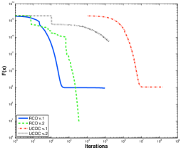
(a) Objective function $F(x)$ against iterations

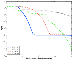
(b) Objective function $F(x)$ against time

Fig. 1: Performance of all four methods RCD v.1 and v.2 and UCDC v.1 and v.2 on a sparse large scale $\ell_{1}$-regularized least squares problem. For practical purposes, for UCDC v.1 results are printed every ten thousand iterations. Calculation of $F(x)$ is not included in running time of the methods. Fig.1a shows how the objective function $F(x)$ decreases as a function of the number of iterations. Fig.1b shows how the objective function $F(x)$ decreases as a function of wall-clock time measured in seconds.

In this figure notice that all methods were terminated after $10^{4}$ seconds. For practical purposes, for UCDC v.1 results are shown every $10^{4}$ iterations. For all other methods results are shown after the first iteration takes place and then at every iteration. Observe in sub Figure 1a that block methods RCD v.1, RCD v.2 and UCDC v.2 performed fewer iterations compared to the single coordinate UCDC v.1. This is due to much larger per iteration computational complexity of the former methods compared to the latter. RCD v.2 despite its larger per iteration computational complexity among all methods it was the only one that solved the problem to higher accuracy within the required maximum time. Moreover, observe in sub Figure 1b that for purely practical purposes it might be better to have a combination of methods RCD v.1 and v.2. The former could be used at the beginning of the process while the latter could be used at later stages in order to guarantee robustness and speed closer to the optimal solution. Finally, it is important to mention that on this problem for both RCD versions unit step sizes $\alpha$ were accepted by the backtracking line search for a major part of the process. Hence, backtracking line search was inexpensive.

6.4 $\ell_{1}$-Regularized Logistic Regression

In this section we present the performance of RCD and UCDC on the $\ell_{1}$-regularized logistic regression problems (48).

Such problems are important in machine learning and are used for training a linear classifier $x\in\mathbb{R}^{N}$ that separates input data into two distinct clusters, for example, see [29] for further details.

We present the performance of the methods on two sparse large scale data sets. Problem details are given in Table 1, where $A\in\mathbb{R}^{m\times N}$ is a matrix whose rows are training samples.

Table 1: Properties of two $\ell_{1}$-regularized logistic regression problems. The second and third columns show the number of training samples and features, respectively. The fourth column shows the sparsity of matrix $A$.

Problem	$\boldsymbol{m}$	$\boldsymbol{N}$	$\mathbf{nnz(A)/(mN)}$
webspam	$350,000$	$16,609,143$	$2.24e$-$4$
kdd2010 (algebra)	$8,407,752$	$20,216,830$	$1.79e$-$6$

The data sets can be downloaded from the collection of LSVM problems in http://www.csie.ntu.edu.tw/~cjlin/libsvmtools/datasets/. For both experiments we set $c=10$, which resulted in more than $99\%$ classification accuracy of the used data sets.

By [20, Table 10], the coordinate Lipschitz constants for UCDC are

$$L_{j}:=\frac{1}{4}\sum_{q=1}^{m}(A_{qj}y_{q})^{2}\quad\forall j=1,2,\cdots,N,$$

where $A_{qj}$ is the component of matrix $A$ at $qth$ row and $jth$ column. For block versions RCD v.1, RCD v.2 and UCDC v.2, we set $\tau=\lceil 0.001N\rceil$.

The result of this experiment is shown in Figure 2.

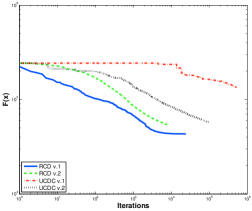
(a) webspam, $F(x)$ against iterations

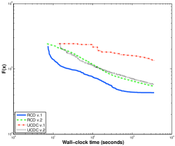
(b) webspam, $F(x)$ against time

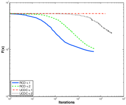
(c) kdda, $F(x)$ against iterations

(d) kdda, $F(x)$ against time

Fig. 2: Performance of all four methods RCD v.1 and v.2 and UCDC v.1 and v.2 on two large scale $\ell_{1}$-regularized logistic regression problems. The first and second rows of figures show the results for problems webspam and kdda, respectively. Calculation of $F(x)$ is not included in running time of the methods.

In this experiment all methods were terminated after one hour of running time. Notice that RCD versions were more efficient than both UCDC versions, with RCD v.1 being the fastest among all. An interesting observation in Figures 2a and 2c is that RCD versions had similar per iteration computational complexity since they performed similar number of iterations within the maximum allowed running time. However, for RCD v.1, it seems that diagonal information from the second order derivatives of $f$ was enough to decrease faster the objective function for all iterations compared to RCD v.2. Finally, in this experiment we observed that both RCD versions accepted unit step sizes for a major part of the process.

7 Conclusion

We presented a robust randomized block coordinate descent method for composite function problems (1), which we name Robust Coordinate Descent (RCD), that can properly handle second-order (curvature) information. The proposed method can vary from first- to second-order; depending on how large the block updates are set, how accurate second-order information are used and how inexactly the arising subproblems are solved. Although the per iteration computational complexity might be higher for RCD, we present synthetic and real world large scale examples where the number of iterations substantially decreases, as well as the overall time.

From the theoretical point of view, we prove global convergence of RCD and under standard assumptions we show that RCD exhibits on expectation block quadratic or superlinear rate of convergence.

References

- [1] P. Alart, O. Maisonneuve, and R. T. Rockafellar. Nonsmooth Mechanics and Analysis: Theoretical and Numerical Advances. Springer US, 2006.
- [2] R. H. Byrd, J. Nocedal, and F. Oztoprak. An inexact successive quadratic approximation method for convex l-1 regularized optimization. Technical report, Northwestern University, September 2013. arXiv:1309.3529v1 [math.OC].
- [3] E. Candès. Compressive sampling. In International Congress of Mathematics, volume 3, pages 1433–1452, Madrid, Spain, 2006.
- [4] E. J. Candés, J. Romberg, and T. Tao. Robust uncertainty principles: Exact signal reconstruction from highly incomplete frequency information. IEEE Trans. Inf. Theory, 52(2):489–509, 2006.
- [5] D. Donoho. Compressed sensing. IEEE Trans. on Information Theory, 52(4):1289–1306, April 2006.
- [6] F. Facchinei, S. Sagratella, and G. Scutari. Parallel algorithms for big data optimization. Technical report, March 2014. arXiv:1402.5521v3 [cs.DC].
- [7] O. Fercoq and P. Richtárik. Accelerated, parallel and proximal coordinate descent. Technical report, University of Edinburgh, December 2013. arXiv:1312.5799v2 [math.OC].
- [8] K. Fountoulakis and J. Gondzio. A second-order method for strongly convex -regularization problems. Technical report, University of Edinburgh, April 2014. arXiv:1306.5386v4 [math.OC].
- [9] R. A. Horn and C. R. Johnson. Matrix Analysis. Cambridge University Press, 1985.
- [10] S. Karimi and S. Vavasis. IMRO: a proximal quasi-Newton method for solving -regularized least square problem. Technical report, University of Waterloo, January 2014. arXiv:1401.4220v1 [math.OC].
- [11] J. D. Lee, Y. Sun, and M. A. Saunders. Proximal Newton-type methods for convex optimization. Advances in Neural Information Processing Systems, pages 836–844, 2012.
- [12] J. D. Lee, Y. Sun, and M. A. Saunders. Proximal Newton-type methods for minimizing composite functions. Technical report, Stanford University, December 2013.
- [13] Z. Lu and L. Xiao. On the complexity analysis of randomized block-coordinate descent methods. Technical report, Simon Fraser University, May 2013. arXiv:1305.4723v1 [math.OC].
- [14] I. Necoara and A. Patrascu. A random coordinate descent algorithm for optimization problems with composite objective function and linear coupled constraints. Computational Optimization and Applications, 57(2):307–337, 2014.
- [15] Yu. Nesterov. Introductory Lectures on Convex Optimization: A Basic Course. Applied Optimization. Kluwer Academic Publishers, 2004.
- [16] Yu. Nesterov. Efficiency of coordinate descent methods on huge-scale optimization problems. SIAM Journal on Optimization, 22(2):341–362, 2012.
- [17] Yu. Nesterov. Gradient methods for minimizing composite functions. Mathematical Programming, 140(1):125–161, 2013.
- [18] J. Nocedal and S. J. Wright. Numerical Optimization. Springer Series in Operations Research. Springer-Verlag, New York, 1999.
- [19] Z. Qin, K. Scheinberg, and D. Goldfarb. Efficient block-coordinate descent algorithms for the group lasso. Mathematical Programming Computation, 5(2):143–169, 2013.
- [20] P. Richtárik and M. Takáč. Iteration complexity of randomized block-coordinate descent methods for minimizing a composite function. Mathematical Programming, 2012.
- [21] P. Richtárik and M. Takáč. Parallel coordinate descent methods for big data optimization. Technical report, University of Edinburgh, December 2013. arXiv:1212.0873v2 [math.OC].
- [22] M. De Santis, S. Lucidi, and F. Rinaldi. A fast active set block coordinate descent algorithm for -regularized least squares. Technical report, March 2014. arXiv:1403.1738v2 [math.OC].
- [23] K. Scheinberg and X. Tang. Practical inexact proximal quasi-Newton method with global complexity analysis. Technical report, Lehigh University, November 2013. arXiv:1311.6547v3 [cs.LG].
- [24] S. Shalev-Schwartz and T. Zhang. Stochastic dual coordinate ascent methods for regularized loss minimization. Journal of Machine Learning Research, 14:567–599, 2013.
- [25] N. Simon and R. Tibshirani. Standardization and the group lasso penalty. Statistica Sinica, 22(3):983, 2012.
- [26] R. Tappenden, P. Richtárik, and J. Gondzio. Inexact coordinate descent: Complexity and preconditioning. Technical report, University of Edinburgh, April 2013. arXiv:1304.5530v1 [math.OC].
- [27] R. Tibshirani. Regression shrinkage and selection via the lasso. Journal of the Roy. Statist. Soc., 58(1):267–288, 1996.
- [28] S. J. Wright. Accelerated block-coordinate relaxation for regularized optimization. SIAM Journal of Optimization, 22(1):159–186, 2012.
- [29] G. X. Yuan, C. H. Ho, and C. J. Lin. Recent advances of large-scale linear classification. Proceedings of the IEEE, 100(9):2584–2603, 2012.