Analysis of Sunyaev-Zel’dovich Effect Mass-Observable Relations using South Pole Telescope Observations of an X-ray Selected Sample of Low Mass Galaxy Clusters and Groups

Abstract

We use microwave observations from the South Pole Telescope (SPT) to examine the Sunyaev-Zel’dovich effect (SZE) signatures of a sample of 46 X-ray selected groups and clusters drawn from $\sim 6~{}\text{deg}^{2}$ of the XMM-Newton Blanco Cosmology Survey (XMM-BCS). These systems extend to redshift $z=1.02$ and probe the SZE signal to the lowest X-ray luminosities ($\geq$10⁴² erg s^-1) yet; these sample characteristics make this analysis complementary to previous studies. We develop an analysis tool, using X-ray luminosity as a mass proxy, to extract selection-bias corrected constraints on the SZE significance- and $Y_{\text{500}}$-mass relations. The former is in good agreement with an extrapolation of the relation obtained from high mass clusters. However, the latter, at low masses, while in good agreement with the extrapolation from the high mass SPT clusters, is in tension at 2.8 $\sigma$ with the Planck constraints, indicating the low mass systems exhibit lower SZE signatures in the SPT data. We also present an analysis of potential sources of contamination. For the radio galaxy point source population, we find 18 of our systems have 843 MHz Sydney University Molonglo Sky Survey (SUMSS) sources within 2 arcmin of the X-ray centre, and three of these are also detected at significance $>$4 by SPT. Of these three, two are associated with the group brightest cluster galaxies (BCGs), and the third is likely an unassociated quasar candidate. We examine the impact of these point sources on our SZE scaling relation analyses and find no evidence of biases. We also examine the impact of dusty galaxies using constraints from the 220 GHz data. The stacked sample provides 2.8 $\sigma$ significant evidence of dusty galaxy flux, which would correspond to an average underestimate of the SPT $Y_{\text{500}}$ signal that is $(17\pm 9)$ per cent in this sample of low mass systems. Finally, we explore the impact of future data from SPTpol and XMM-XXL, showing that it will lead to a factor of four to five tighter constraints on these SZE mass-observable relations.

1 Introduction

The Sunyaev-Zel’dovich effect (Sunyaev & Zel’dovich, 1970, 1972, SZE), is a spectral distortion of the cosmic microwave background (CMB) arising from interactions between CMB photons and hot, ionised gas. Surveys of galaxy clusters using the SZE have opened a new window on the Universe by providing samples of hundreds of massive galaxy clusters with well-understood selection over a broad redshift range. Both space- and ground-based instruments, including the Planck satellite (Tauber et al., 2010), the South Pole Telescope (SPT; Carlstrom et al., 2011), and the Atacama Cosmology Telescope (ACT; Fowler et al., 2007), have released catalogs of their SZE selected clusters. The cluster samples have provided new cosmological constraints Reichardt et al. (2013); Hasselfield et al. (2013); Planck Collaboration (2013a) and have enabled important evolution studies of cluster galaxies and the intracluster medium over a broad range of redshift (e.g., Zenteno et al., 2011; Semler et al., 2012; McDonald et al., 2013).

Understanding the relationship between the SZE observable and cluster mass is important for both cosmological applications and astrophysical studies. Among observables, the integrated Comptonization from the SZE has been shown by numerical simulations Motl et al. (2005); Nagai et al. (2007) to be a good mass proxy with low intrinsic scatter. Cluster mass estimates derived from X-ray observations of SZE selected clusters have largely confirmed this expectation Andersson et al. (2011); Planck Collaboration (2011a). A related quantity, the SPT signal-to-noise $\xi$, is linked to the underlying virial mass of the cluster by a power law with log-normal scatter at the $\sim 20$ per cent level (Benson et al., 2013, hereafter B13).

Probing the SZE signature of low mass clusters and groups is also important, although it is much more challenging with the current generation of experiments. These low mass clusters and groups are far more numerous and are presumably important environments for the transformation of galaxies from the field to the cluster. Studies of their baryonic content show that low mass clusters and groups are not simply scaled-down versions of the more massive clusters (e.g., Mohr et al., 1999; Sun et al., 2009; Laganá et al., 2013). This breaking of self-similarity in moving from the cluster to the group mass scale is likely due to processes such as star formation and active galactic nucleus (AGN) feedback.

The Planck team has recently studied this low mass population by stacking the Planck maps around samples of X-ray selected clusters in the nearby universe (Planck Collaboration, 2011b, hereafter P11). They show that the SZE signal is consistent with the self-similar scaling relation based on the X-ray luminosity over a mass range spanning 1.4 orders of magnitude.

Here we pursue a study of the SZE signatures of low mass clusters extending over a broad range of redshift. We use the South Pole Telescope Sunyaev-Zel’dovich survey (SPT-SZ) data with the XMM-BCS over $6~{}\text{deg}^{2}$ from which a sample of 46 X-ray groups and clusters have been selected (Šuhada et al., 2012, hereafter S12). The SPT-SZ data enable us to extract cluster SZE signal with high angular resolution and low instrument noise, making the most of this small sample.

The paper is organised as follows. In sec:xbcs-data-description, we describe the data used from the XMM-BCS and the extraction of the SZE signature from the SPT-SZ maps. In sec:xbcs-method, we introduce the calibration method for the mass-observable scaling relation, and we apply it to the cluster sample in sec:xbcs-result. We also discuss possible systematic effects and present a discussion of the point source population associated with our sample. We conclude in sec:xbcs-conclusions with a prediction of the improvement based on future surveys.

The cosmological model parameters adopted in this paper are the same as the ones used for the X-ray measurement from the XMM-BCS project (S12): $(\Omega_{\mathrm{M}},\Omega_{\Lambda},H_{0})=(0.3,0.7,70~{}\text{km s}^{-1}\text{Mpc}^{-1})$. The amplitude of the matter power spectrum, which is needed to estimate bias corrections in the analysis, is fixed to $\sigma_{8}=0.8$.

2 Data Description and Observables

In this analysis, we adopt an X-ray selected sample of clusters, described in sec:xbcs-xmmbcs, together with published $L_{\text{X}}$-mass scaling relations to examine the corresponding SPT-SZ significance- and $Y_{\text{500}}$-mass relations. The SPT-SZ observable $\xi$ is measured by a matched filter approach, which we discuss in sec:xbcs-spt and sec:xbcs-spt-xi. The estimation of $Y_{\text{500}}$ is described in sec:xbcs-yintegrated.

2.1 X-ray Catalog

The XMM-BCS project consists of an X-ray survey mapping $14~{}\text{deg}^{2}$ area of the southern hemisphere sky that overlaps the griz bands Blanco Cosmology Survey (Desai et al., 2012, BCS) and the mm-wavelength SPT-SZ survey Carlstrom et al. (2011). S12 analyse the initial $6~{}\text{deg}^{2}$ core area, construct a catalog of 46 galaxy clusters and present a simple selection function. Here we present a brief summary of the characteristics of that sample. The cluster physical parameters from Table 2 (S12) are repeated in tab:xbcs-cat with the same IDs.

The initial cluster sample was selected via a source detection pipeline in the 0.5–2 keV band. The spatial extent of the clusters leads to the need to have more counts to reach a certain detection threshold than are needed for point sources. S12 modelled the extended source sensitivity as an offset from the point source limit; the cluster sample is approximately a flux-limited sample with $f_{\text{min}}=1\times 10^{-14}\text{erg s}^{-1}\text{cm}^{-2}$.

The X-ray luminosity $L_{\text{X}}$ was measured in the detection band (0.5 - 2.0 keV) within a radius of $R_{\text{500c}}$, which is iteratively determined using mass estimates from the $L_{\text{X}}$-mass relation and is defined such that the interior density is 500 times the critical density of the Universe at the corresponding redshift. This luminosity was converted to a bolometric luminosity and to a 0.1 - 2.4 keV band luminosity using the characteristic temperature for a cluster with this 0.5 - 2.0 keV luminosity and redshift (see equation 3 in S12). The core radius, $R_{\text{c}}$, of the beta model is calculated using (see equation 1 in S12):

$$R_{\text{c}}=0.07\times R_{500}\Big{(}\frac{T}{\text{1~{}keV}}\Big{)}^{0.63},$$ (1)

where $T$ is X-ray temperature determined through the $L_{\text{X}}-T$ relation. The redshifts of the sample are primarily photometric redshifts extracted using the Blanco Cosmology Survey (BCS) optical imaging data. The optical data and their processing and calibration are described in detail elsewhere Desai et al. (2012). The photometric redshift estimator has been demonstrated on clusters with spectroscopic redshifts and on simulations Song et al. (2012a) and has been used for redshift estimation within the SPT-SZ collaboration Song et al. (2012b). The typical photometric redshift uncertainty in this XMM-BCS sample is $\langle\Delta z/(1+z)\rangle=0.023$, which is determined using a subsample of 12 clusters ($z<0.4$) with spectroscopic redshifts. This value is consistent with the uncertainty $\langle\Delta z/(1+z)\rangle=0.017$ we obtained on the more massive main sample SPT-SZ clusters.

The X-ray luminosities and photometric redshifts of the sample are shown in fig:xbcs-lxza in black squares and the approximate flux limit of the sample is shown as a red curve. For comparison, we also include a high mass SPT-SZ cluster sample (blue triangles) with published X-ray properties Andersson et al. (2011).

In the analysis that follows we use the X-ray luminosity as the primary mass estimator for each cluster. We adopt the $L_{\text{X}}$-mass scaling relation used in S12, which is based on the hydrostatic mass measurements in an ensemble of 31 nearby clusters observed with XMM-Newton (REXCESS, Pratt et al., 2009):

$$L_{\text{X}}=L_{0}\Big{(}\frac{M_{\text{500c}}}{2\times 10^{14}\mathrm{M_{\odot}}}\Big{)}^{\alpha_{\text{LM}}}E(z)^{7/3},$$ (2)

where $H(z)=H_{0}E(z)$. The intrinsic scatter in $L_{\text{X}}$ at fixed mass is modelled as lognormal distributions with widths $\sigma_{L_{\text{X}}}$, and the observational scatter is given in S12.

This scaling relation includes corrections for Malmquist and Eddington biases. Both biases are affected by the intrinsic scatter and the skewness of the underlying sample distribution. In general, the bias on the true mass is $\Delta\ln M\ \propto\ \gamma\sigma_{\ln M}^{2}$, where $\mathrm{d}n(M)/\mathrm{d}\ln M\propto M^{\gamma}$ is the slope of the mass distribution and $\sigma_{\ln M}$ is the scatter in mass at fixed observable (for more discussion, we refer the reader to Stanek et al., 2006; Vikhlinin et al., 2009; Mortonson et al., 2011). Typically $\gamma$ is negative, and the result is that mass inferred from an observable must be corrected to a lower value than that suggested by naive application of the scaling relation.

The scaling relation parameters for different X-ray bands are listed in tab:xbcs-lxm. We find the choice of luminosity bands has negligible impact on the parameter estimation given the current constraint precision. In addition, we investigate using the $L_{\text{X}}$-mass scaling relations from Chandra observations (Vikhlinin et al., 2009; Mantz et al., 2010a). These studies draw upon higher mass cluster samples than the REXCESS sample, and therefore we adopt the Pratt et al. (2009) relation for our primary analysis. We discuss the impact of changing the $L_{\text{X}}$-mass scaling relation in sec:xbcs-xim.

Table 1: $L_{\text{X}}$-mass relations with different luminosity bands (eq:xbcs-lm).

Type	$L_{0}[10^{44}\text{erg\ s}^{-1}]$	$\alpha_{\text{LM}}$	$\sigma_{\ln L_{\text{X}}}$
0.5–2.0 keV	$0.48\pm 0.04$	$1.83\pm 0.14$	$0.412\pm 0.071$
0.1–2.4 keV	$0.78\pm 0.07$	$1.83\pm 0.14$	$0.414\pm 0.071$
Bolometric	$1.38\pm 0.12$	$2.08\pm 0.13$	$0.383\pm 0.061$

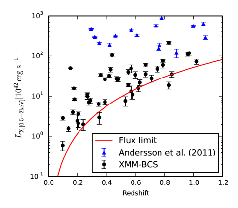
Figure 1: The luminosity-redshift distribution of the XMM-BCS clusters from S12 (black dots) and the SPT-SZ clusters from Andersson et al. (2011, blue triangles). The X-ray sample is selected with a flux cut that varies somewhat across the field. The red line is the corresponding luminosity sensitivity determined by the median flux limit in the 0.5 - 2.0 keV band. The SPT-SZ sample is more massive and approximately mass limited.

2.2 SPT Observations

The SPT (Carlstrom et al., 2011) is a 10-metre diameter, millimetre-wavelength, wide field telescope that was deployed in 2007 and has been used since then to make arcminute-resolution observations of the CMB over large areas of the sky. The high angular resolution is crucial to detecting the SZE signal from high-redshift clusters. The SPT-SZ survey (e.g., Story et al., 2013), completed in 2011, covers a 2500 deg² region of contiguous sky area in three bands – centred at 95, 150, and 220 GHz – at a typical noise level of $<18\mu$K per one-arcminute pixel in the 150 GHz band.

The details of the SPT-SZ observation strategy, data processing and mapmaking are documented in Schaffer et al. (2011); we briefly summarise them here. The SPT-SZ survey data were taken primarily in a raster pattern with azimuth scans at discrete elevation steps. A high-pass filter was applied to the time-ordered data to remove low-frequency atmospheric and instrumental noise. The beams, or angular response functions, were measured using observations of planets and bright AGNs in the field. The main lobe of the beam for a field observation is well-approximated as a Gaussian with a full-width half maximum (FWHM) of 1.6, 1.2, and 1.0 arcmin at 95, 150, and 220 GHz, respectively. The final temperature map was calibrated by the Galactic H II regions RCW38 and MAT5a (c.f. Vanderlinde et al., 2010). The SPT-SZ maps used in this work are from a 100 deg² field centred at $(\alpha,\delta)$ = $(23^{\circ}\ 30^{\prime},-55^{\circ})$ and consist of observations from the 2008 and 2010 SPT-SZ observing seasons. The characteristic depths are 37, 12 and $35~{}\mu\text{K-arcmin}$ at 95, 150 and 220 GHz, respectively.

2.3 SPT-SZ Cluster Significance

The process of determining the SPT-SZ significance for our X-ray sample is very similar to the process of finding clusters in SPT-SZ maps, but there are certain key differences, which we highlight below. Clusters of galaxies are extracted from SPT-SZ maps through their distinct angular scale- and frequency-dependent imprint on the CMB. We adopt the multi-frequency matched filter approach Melin et al. (2006) to extract the cluster signal. The matched filter is designed to maximise the given signal profile while suppressing all noise sources. A detailed description appears elsewhere (Vanderlinde et al., 2010; Williamson et al., 2011). Here we provide a summary. The SZE introduces a spectral distortion of the CMB at given frequency $\nu$ as:

$$\Delta T_{\text{CMB}}(\bm{\theta},\nu)=y(\bm{\theta})g(\nu)T_{\text{CMB}},$$ (3)

where $g(\nu)$ is the frequency dependency and the Compton-y parameter $y(\bm{\theta})$ is the SZE signature at direction $\bm{\theta}$, which is linearly related to the integrated pressure along the line-of-sight. To model the SZE signal $y(\bm{\theta})$, two common templates are adopted: the circular $\beta$ model Cavaliere & Fusco-Femiano (1976) and the Arnaud profile Arnaud et al. (2010). The cluster profiles are convolved with the SPT beams to get the expected signal profiles. The map noise assumed in constructing the filter includes the measured instrumental and atmospheric noise and sources of astrophysical noise, including the primary CMB. Point sources are identified in a similar manner within each band independently, using only the instrument beams as the source profile Vieira et al. (2010).

Once SPT-SZ maps have been convolved with the multi-frequency matched filter, clusters are extracted with a simple peak-finding algorithm, with the primary observable $\xi$ defined as the maximum signal-to-noise of a given peak across a range of filter scales. The SPT-SZ significance $\xi$ is a biased estimator that links to the underlying $\zeta$ as $\langle\xi\rangle=\sqrt{\zeta^{2}+3}$, because it is the maximum value identified through a search in sky position and filter angular scale (Vanderlinde et al., 2010). The observational scatter of $\xi$ around $\zeta$ is a unit-width Gaussian distribution corresponding to the underlying RMS noise of the SPT-SZ filtered maps.

In this work, we use the 90 GHz and 150 GHz maps and employ the method described above to define an SPT-SZ significance for each X-ray selected cluster, but with two important differences: 1) We measure the SPT-SZ significance at the X-ray location, and 2) we use a cluster profile shape informed from the X-ray data. We define this SPT-SZ significance as $\xi_{\text{X}}$, which is related to the unbiased SPT-SZ significance $\zeta$ as:

$$\zeta=\langle\xi_{\text{X}}\rangle,$$ (4)

where the angle brackets denote the average over many realizations of the experiment. The observational scatter of $\xi_{\text{X}}$ around $\zeta$ is also a unit-width Gaussian distribution. Therefore $\xi_{\text{X}}$ is an unbiased estimator of $\zeta$, under the assumption that the true X-ray position and profile are identical to the true SZE position and profile – a reasonable assumption – given that both the X-ray and the SZE signatures are reflecting the intracluster medium properties of the clusters. Note, however, that in the midst of a major merger the different density weighting of the X-ray and SZE signatures can lead to offsets (Molnar et al., 2012).

We model the relationship between $\zeta$ and the cluster mass through

$$\zeta=A_{\text{SZ}}^{\text{SPT}}\Big{(}\frac{M_{\text{500c}}}{4.3\times 10^{14}\mathrm{M_{\odot}}}\Big{)}^{B_{\text{SZ}}}\Big{[}\frac{E(z)}{E(0.6)}\Big{]}^{C_{\text{SZ}}},$$ (5)

where the intrinsic scatter on $\zeta$ is described by a log-normal distribution of width $D_{\text{SZ}}$ (B13; Reichardt et al., 2013). We use $A_{\text{SZ}}^{\text{SPT}}$ to denote the amplitude of the original SPT-SZ scaling relation. The differences in the depths of the SPT-SZ fields results in a re-scaling of the SPT-SZ cluster significance in spatially filtered maps. For the field we study here, the relation requires a factor of 1.38 larger normalisation compared to the value in Reichardt et al. (2013).

For the massive SPT-SZ clusters (with $\xi>4.5$), the $\zeta$-mass relation is best parametrized as shown in tab:xbcs-constraint with $C_{\text{SZ}}=0.83\pm 0.30$ and $D_{\text{SZ}}=0.21\pm 0.09$ (B13). In our analysis, we examine the characteristics of the lower mass clusters within the SPT-SZ survey. To avoid a degeneracy between the scaling relation amplitude and slope, we shift the pivot mass to $1.5\times 10^{14}~{}\mathrm{M_{\odot}}$, near the median mass of our sample and term the associated amplitude $A_{\text{SZ}}$. At this pivot mass, with the normalisation factor mentioned previously, the equivalent amplitude parameter for the main SPT-SZ sample corresponds to $A_{\text{SZ}}=1.50$. In tab:xbcs-constraint we also note the priors we adopt in our analysis of the low mass sample. For our primary analysis we adopt flat priors on the amplitude and slope parameters and fix the redshift evolution and scatter at the values obtained by B13.

2.4 Integrated $Y_{\text{500}}$

To facilitate the comparison of our sample with cluster physical properties reported in the literature, we also convert the $\xi_{\text{X}}$ to $Y_{\text{500}}$, which is the integration of the Compton-y parameter within a spherical volume with radius $R_{\text{500c}}$. The central $y_{0}$ is linearly linked to $\xi_{\text{X}}$ in the matched filter approach (Melin et al., 2006), with the corresponding Arnaud profile or $\beta$ profile as the cluster template. The characteristic radii ($R_{\text{500c}}$ and $R_{\text{c}}$) are based on the X-ray measurements (S12), because the SZE observations are too noisy to constrain the profile accurately.

The projected circular $\beta$ profile for the filter is:

$$y^{\mathrm{(\beta)}}_{\text{cyl}}(r)\propto(1-r^{2}/R_{\text{c}}^{2})^{-(3\beta-1)/2},$$ (6)

where $\beta$ is fixed to 1, consistent with higher signal to noise cluster studies (Plagge et al., 2010). And the spherical $Y_{\text{500}}$ within the $R_{\text{500c}}$ is

$$Y_{\text{500}}^{\mathrm{(\beta)}}=y_{0}\times\pi R_{\text{c}}^{2}\ln(1+R_{\text{500c}}^{2}/R_{\text{c}}^{2})\times f(R_{\text{500c}}/R_{\text{c}}),$$ (7)

where $f(x)$ corrects the cylindrical result to the spherical value for the $\beta$ profile as:

$$f(x)=2\frac{\ln(x+\sqrt{1+x^{2}})-x/\sqrt{1+x^{2}}}{\ln(1+x^{2})}.$$ (8)

The $Y_{\text{500}}^{\text{(A)}}$ for the Arnaud profile is calculated similarly except that the projected profile is calculated numerically within $5R_{\text{500c}}$ along the line-of-sight direction:

$$y^{\text{(A)}}_{\text{cyl}}(r)\propto\int_{-5R_{\text{500c}}}^{5R_{\text{500c}}}P\Big{(}\frac{\sqrt{r^{2}+z^{2}}}{R_{\text{500c}}}\Big{)}\mathrm{d}z,$$ (9)

where the pressure profile has the form

$$P(x)\propto(c_{\text{500}}x)^{-\gamma_{\text{A}}}[1+(c_{\text{500}}x)^{\alpha_{\text{A}}}]^{(\gamma_{\text{A}}-\beta_{\text{A}})/\alpha_{\text{A}}},$$ (10)

with $[c_{\text{500}},\gamma_{\text{A}},\alpha_{\text{A}},\beta_{\text{A}}]=[1.177,0.3081,1.0510,5.4905]$ Arnaud et al. (2010). The integration up to $5R_{\text{500c}}$ includes more than 99 per cent of the total pressure contribution. The spherical $Y_{\text{500}}$ for the Arnaud profile is:

$$Y_{\text{500}}^{\text{(A)}}=2\pi y_{0}\int_{0}^{R_{\text{500c}}}y^{\text{(A)}}_{\text{cyl}}(r)r\mathrm{d}r/1.203,$$ (11)

where the numerical factor 1.203 is the ratio between cylindrical integration and spherical integration for the adopted Arnaud profile parameters.

Measurements of $Y_{\text{500}}$ are sensitive to the assumed profile. The Arnaud profile depends only on $R_{\text{500c}}$, while the $\beta$ profile depends on both $R_{\text{500c}}$ and $R_{\text{c}}$ and therefore $Y_{\text{500}}$ is sensitive to the ratio $R_{\text{c}}/R_{\text{500c}}$. We find that with $R_{\text{c}}/R_{\text{500c}}=0.2$ the $\beta$ and Arnaud profiles provide $Y_{\text{500}}$ measurements in good agreement; this ratio is consistent with the previous SZE profile study using high mass clusters (Plagge et al., 2010). Interestingly, the X-ray data indicate a characteristic ratio of $0.11\pm 0.03$ for our sample, and a shift in the $R_{\text{c}}/R_{\text{500c}}$ ratio from 0.2 to 0.1 leads to a $\sim$40 per cent decrease in $Y_{\text{500}}$. Given that the Planck analysis to which we compare is carried out using the Arnaud profile, we adopt that profile for the analysis in Section 4.4 below.

The $Y_{\text{500}}$-mass scaling relation has been modelled using a representative local X-ray cluster sample Arnaud et al. (2010) and further studied in the SZE (Andersson et al., 2011, P11) as

$$Y_{\text{500}}=A_{\text{Y}}\Big{(}\frac{M_{500}}{1.5\times 10^{14}M_{\odot}}\Big{)}^{B_{\text{Y}}}E(z)^{2/3}\Big{[}\frac{D_{\text{A}}(z)}{500\text{Mpc}}\Big{]}^{-2},$$ (12)

where $D_{\text{A}}(z)$ is the angular-diameter distance and the intrinsic scatter on $Y_{\text{500}}$ is described by a log-normal distribution of width $\sigma_{\mathrm{\ln Y}}=0.21$. The observational scatter of $Y_{\text{500}}$ is propagated from the scatter of $\xi_{\text{X}}$. In sec:xbcs-result, we fit this relation to the observations.

3 Method

In this section, we describe the method we developed to fit the SZE-mass scaling relations of the low mass cluster population selected through the XMM-BCS and observed by the SPT. In principle, we could use our cluster sample observed in X-ray and SZE to simultaneously constrain the cosmology and the scaling relations, in the so-called self-calibration approach Majumdar & Mohr (2004). However, self-calibration requires a large sample. Without this, we take advantage of strong, existing cosmology constraints (e.g., Planck Collaboration, 2013b; Bocquet et al., 2014) and knowledge of the $L_{\text{X}}$-mass scaling relation (e.g. Pratt et al., 2009). We focus only on the SZE-mass scaling relations, exploring the SZE characteristics of low mass galaxy clusters and groups. In sec:xbcs-lik we present the method and in sec:xbcs-submocks we validate it using mock catalogs.

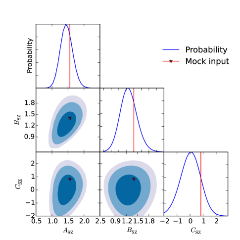
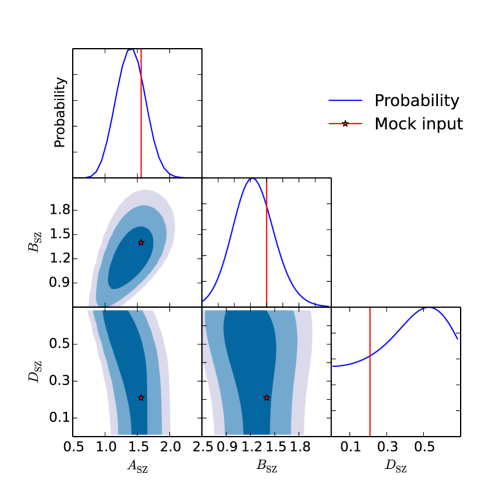
Figure 2: Constraints on the $\zeta$-mass relation from an analysis of the mock catalog. The left panel constrains $A_{\text{SZ}}$, $B_{\text{SZ}}$, and $C_{\text{SZ}}$ with fixed $D_{\text{SZ}}$. And the right panel shows the result by fixing $C_{\text{SZ}}$ instead of $D_{\text{SZ}}$. The red lines and stars denote the input values of the scaling relation parameters of the mock catalog. Histograms in each case show the recovered projected likelihood distribution for each parameter. Joint constraints for different pairs of parameters are shown in blue with different shades indicating the 1, 2, and 3$\,\sigma$ levels.

3.1 Description of the Method

The selection biases on scaling relations include the Malmquist bias and the Eddington bias, which are manifestations of scatter and population variations associated with the selection observable. Several methods have previously been developed (e.g., Vikhlinin et al. 2009; Mantz et al. 2010b; Allen et al. 2011; B13; Bocquet et al. 2014) to account for the sampling biases when fitting scaling relation and cosmological parameters simultaneously. In this analysis, we use a likelihood function that can be derived from the one presented in B13. For a detailed discussion we refer the reader to Appendix A; here we present an overview of the key elements of this likelihood function.

The likelihood function $\mathcal{L}(\bm{r}_{\text{SZ}})$ we use to constrain the SZE-mass relations is the product of the individual conditional probabilities to observe each cluster with SZE observable $Y_{i}$ (e.g., SPT-SZ significance $\xi_{\text{X}}$ or $Y_{\text{500}}$), given the cluster has been observed to have an X-ray observable $L_{i}$ and redshift $z_{i}$:

$$\mathcal{L}(\bm{r}_{\text{SZ}})=\Pi_{i}\ P(Y_{i}|L_{i},z_{i},\bm{c},\bm{r}_{\text{X}},\bm{r}_{\text{SZ}},\Theta_{\text{X}}),$$ (13)

where $i$ runs over the cluster sample, $\bm{r}_{\text{SZ}}$ contains the parameters describing the SZE mass-observable scaling relation that we wish to study, $\bm{c}$ contains the cosmological parameters, $\bm{r}_{\text{X}}$ contains the parameters describing the X-ray mass-observable scaling relation, and the survey selection in X-ray is encoded within $\Theta_{\text{X}}$. Note that the redshifts are assumed to be accurate such that the X-ray luminosity ($L_{\text{X}}$) is used instead of the true survey selection observable, which is the X-ray flux.

As noted above, given the size of our dataset we adopt fixed cosmology $\bm{c}$ and X-ray scaling relation parameters $\bm{r}_{\text{X}}$ to focus on the SZE-mass scaling relation. In sec:xbcs-result we examine the sensitivity of our results to the current uncertainties in cosmology and the X-ray scaling relation and find them to be unimportant for our analysis. Within this context, the conditional probability density function for cluster $i$ can be written as the ratio of the expected number of clusters $\mathrm{d}N$ with observables $Y_{i}$, $L_{i}$ and $z_{i}$ within infinitesimal volumes $\mathrm{d}Y$, $\mathrm{d}L$ and $\mathrm{d}z$:

$$P(Y_{i}|L_{i},z_{i},\bm{r}_{\text{SZ}},\Theta_{\text{X}})=\frac{\mathrm{d}N(Y_{i},L_{i},z_{i}|\bm{r}_{\text{SZ}},\Theta_{\text{X}})}{\mathrm{d}N(L_{i},z_{i}|\Theta_{\text{X}})},$$ (14)

where we have dropped the cosmology $\bm{c}$ and X-ray scaling relation parameters $\bm{r}_{\text{X}}$ because they are held constant. Typically, the survey selection $\Theta_{\text{X}}$ is a complex function of the redshift and X-ray flux, but in the above expression it is simply the probability that a cluster with X-ray luminosity $L_{i}$ and redshift $z_{i}$ is observed (i.e. $\mathrm{d}N\left(Y_{i},L_{i},z_{i}|\bm{r}_{\text{SZ}},\Theta_{\text{X}}\right)=\Theta_{\text{X}}(L_{i},z_{i})\mathrm{d}N(Y_{i},L_{i},z_{i}|\bm{r}_{\text{SZ}})$); in eq:xbcs-single-like this same factor appears in both the numerator and denominator, and therefore it cancels out. Thus, studying the SZE properties of an X-ray selected sample does not require detailed modelling of the selection. If the selection were based on both $L$ and $Y$, then there would be no cancellation, because the selection probability in the numerator would be just $\Theta(L_{i},Y_{i},z_{i})$ while in the denominator it would have to be marginalised over the unobserved $Y$ as $\int\Theta(Y,L_{i},z_{i})\mathrm{d}Y$ (see eq:xbcs-selection-yl).

With knowledge of the cosmologically dependent mass function $n(M,z)\equiv\mathrm{d}N(M,z|\bm{c})/\mathrm{d}M\mathrm{d}z$ Tinker et al. (2008), the ratio of the expected number of clusters can be written as:

$$P(Y_{i}|L_{i},z_{i},\bm{r}_{\text{SZ}})=\frac{\int\mathrm{d}MP(Y_{i},L_{i}|M,z_{i},\bm{r}_{\text{SZ}})\,n(M,z_{i})}{\int\mathrm{d}MP(L_{i}|M,z_{i})\,n(M,z_{i})}.$$ (15)

We emphasise that there is a residual dependence on the X-ray selection in our analysis in the sense that we can only study the SZE properties of the clusters that have sufficient X-ray luminosity to have made it into the sample. This effectively limits the mass range over which we can use the X-ray selected sample to study the SZE properties of the clusters.

To constrain the scaling relation in the presence of both observational uncertainties and intrinsic scatter, we further expand the conditional probability density functions in Equation (15):

$$P(Y_{i},L_{i}|M,z_{i},\bm{r}_{\text{SZ}})=\iint \mathrm{d}Y_{\mathrm{t}}\mathrm{d}L_{\mathrm{t}}\ P(Y_{i},L_{i}|Y_{\mathrm{t}},L_{\mathrm{t}})$$

$$\times P(Y_{\mathrm{t}},L_{\mathrm{t}}|M,z_{i},\bm{r}_{\text{SZ}}),$$ (16)

$$P(L_{i}|M,z_{i})=\int \mathrm{d}L_{\mathrm{t}}\ P(L|L_{\mathrm{t}})P(L_{\mathrm{t}}|M,z_{i}),$$ (17)

where, as above, $Y_{i}$ and $L_{i}$ are the observed values, and $Y_{\mathrm{t}}$ and $L_{\mathrm{t}}$ are the true underlying observables related to mass through scaling relations that have intrinsic scatter. The first factor in each integral represents the measurement error, and the second factor describes the relationship between the pristine observables and the halo mass. Improved data quality affects the first factor, but cluster physics dictates the form of the second. These second factors are fully described by the power law mass-observable relations in Equations (2), (5), and (12) together with the adopted log-normal scatter.

We use this likelihood function under the assumption that there is no correlated scatter in the observables; in sec:xbcs-submocks we use mock samples that include correlated scatter to examine the impact on our results.

3.2 Validation with Mock Cluster Catalogs

We use mock samples of clusters to validate our likelihood and fitting approach and to explore our ability to constrain different parameters. Specifically, we generate ten larger mock surveys of 60 $\text{deg}^{2}$, with a similar flux limit of $1\times 10^{-14}\text{erg s}^{-1}\text{cm}^{2}$ and $z>0.2$. Each mock catalog contains $\sim 400$ clusters, or approximately eight times as many as in the observed sample. The $\xi_{\text{X}}$ of the sample spans $-2.2\leq\xi_{\text{X}}\leq 7.8$ with a median value of $1.4$. We include both the intrinsic scatter and observational uncertainties for both the $L_{\text{X}}$ and the $\xi_{\text{X}}$ in the mock catalog. The intrinsic scatter is lognormal distributed with values given as $\sigma_{\ln L_{\text{X}}}$ ($D_{\text{SZ}}$). The observational uncertainties in $L_{\text{X}}$ and $\xi_{\text{X}}$ are modelled as normal distributions. The standard deviation used for $L_{\text{X}}$ is proportional to $\sqrt{L_{\text{X}}}$ to mimic the Poisson distribution of photon counts, while the standard deviation for $\xi_{\text{X}}$ is 1.

Here we focus on recovering the four SPT-SZ $\zeta$-mass relation parameters from the mock catalog; the fiducial values for these parameters are the B13 best-fitting values. We scan through the parameter space using a fixed grid. The following results contain 41 bins in each parameter direction. Given the limited constraining power, we validate the parameters using two different sets of priors. In the first set we adopt flat priors on $A_{\text{SZ}}$, $B_{\text{SZ}}$, and $C_{\text{SZ}}$ with fixed $D_{\text{SZ}}$. In the second set we adopt flat positive priors on $A_{\text{SZ}}$, $B_{\text{SZ}}$, and $D_{\text{SZ}}$ with fixed $C_{\text{SZ}}$. All other relevant parameters are fixed, including the $L_{\text{X}}$-mass scaling and the cosmological model.

Our tests show good performance of the method. Using ten mock samples that are each ten times larger than our observed sample, and fitting for 3 parameters in each mock, we recover the parameters to within the marginalised $1\,\sigma$ statistical uncertainty 70 per cent of the time and to within $2\,\sigma$ for the rest. fig:xbcs-mock-test illustrates our $\zeta$-mass parameter constraints from one mock sample. Note that the constraints on $C_{\text{SZ}}$ and $D_{\text{SZ}}$ are both weak and exhibit no significant degeneracy with the other two SPT-SZ scaling parameters. We take this as motivation to fix $C_{\text{SZ}}$ and $D_{\text{SZ}}$ and focus on the amplitude $A_{\text{SZ}}$ and slope $B_{\text{SZ}}$ in the analysis of the observed sample. We have repeated this testing in the case of the $Y_{\text{500}}$-mass relation, and we see no difference in behavior.

We also investigate the sensitivity of our method when a correlation between intrinsic scatter in the X-ray and $\xi_{\text{X}}$ is included. Cluster observables can be correlated through an analysis approach. For example, if one uses the $L_{\text{X}}$ as a virial mass estimate, then when $L_{\text{X}}$ scatters up by 40 per cent, it leads to a 5 per cent increase in radius, and 8 per cent increase in $Y_{\text{500}}$ if the underlying SZE brightness distribution is described by the Arnaud et al. (2010) profile. In comparison, the intrinsic scatter of $Y_{\text{500}}$ about mass is about 20 per cent, which in this example would still dominate over the correlated component of the scatter. Correlated scatter in different observable-mass relations can also reflect underlying physical properties of the cluster that impact the two observables in a similar manner.

We find that even with a correlation coefficient $\rho=0.5$ between the intrinsic scatter of the two observables, the change in constraints extracted using a no correlation assumption is small. Thus, our approximation does not lead to significant bias in the analysis of this sample. This result is also consistent with the fact that by extending Equations (16) and (17) to include multi-dimensional log-normal scatter distributions, we find the constraint on correlated scatter in the mock catalog to be very weak. We therefore do not include the possibility of correlated scatter when studying the real sample.

4 Results

In this section, we present the observed relationship between the SZE significance $\xi_{\text{X}}$ at the position of the X-ray selected cluster and the predicted value given the measured X-ray luminosity of the system. Thereafter, we test – and rule out – the null hypothesis that the SZE signal at the locations of the X-ray selected clusters is consistent with noise. We then present constraints on the SPT-SZ $\zeta$-mass and $Y_{\text{500}}$-mass relations. We end with a discussion of possible systematics and a presentation of the point source population for this X-ray selected group and cluster sample.

4.1 SPT Significance Extraction

We extract the $\xi_{\text{X}}$ from the SPT-SZ multi-frequency-filtered map at the location of each XMM-BCS selected cluster as described in sec:xbcs-data-description. In the primary analysis, we adopt three matched-filtered maps from the SPT-SZ data, one each for $\beta$-model profiles with $R_{\text{c}}=$ 0.25, 0.5, and 0.75 arcmin, and we extract the value of $\xi_{\text{X}}$ for each cluster from the map that most closely matches the X-ray-derived $R_{\text{c}}$ value for that cluster. The $\xi_{\text{X}}$ is extracted at the X-ray-derived cluster position. The measured $\xi_{\text{X}}$ values are presented in tab:xbcs-cat. We have also tried extracting SPT-SZ significance by making a matched-filtered map for every cluster, using a filter with the exact X-ray-derived value of $R_{\text{c}}$, and the change in the results is negligible.

We have also investigated the dependence of $\xi_{\text{X}}$ on the assumed cluster profile. We repeated the analysis described above using the Arnaud profile and a $\beta$ profile with $\beta=2/3$. The resulting changes in the extracted values of $\xi_{\text{X}}$ are less than 3 per cent of the measurement uncertainty on the individual $\xi_{\text{X}}$ values. A similar lack of sensitivity to the assumed cluster profile is seen in the $\xi>5$ SPT-SZ derived cluster samples.

The cluster with the strongest detection in the SPT-SZ maps is illustrated in fig:xbcs-clu044, which contains a pseudo-colour optical image with SPT-SZ signal-to-noise contours in white. The SPT-SZ significance, $\xi$, of this cluster is 6.23 corresponding to maximum signal-to-noise in the filtered map (SPT-CLJ2316-5453, Bleem et al. in prep.), whereas the $\xi_{\text{X}}$ is 4.58 at the X-ray position with $R_{\text{c}}$ of 0.367 arcmin. This reduction in signal to noise is expected because there is noise in the SZE map, and the SPT-SZ cluster is selected to lie at the peak $\xi$.

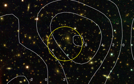
Figure 3: BCS optical pseudo-colour image of cluster 044 in gri bands. The yellow circle (1.5 arcmin diameter) centred at the X-ray peak indicates the rough size of the SPT beam (1.2 arcmin FWHM in 150 GHz and 1.6 arcmin in 95 GHz). The SPT-SZ filtered map is overlaid with white contours, which are marked with the significance levels. The offset between the X-ray centre and the SZE peak is $0.75$ arcmin, and the BCG for this system lies near those two centres.

Table 2: SPT-SZ $\xi_{\text{X}}$ of XMM-BCS sample.

ID	$L_{\mathrm{X,500,bol}}$ $[10^{42}~{}\text{erg/s}]$	$\Delta L_{\mathrm{X,500,bol}}$ $[10^{42}~{}\text{erg/s}]$	Redshift	Redshift uncertainty	$R_{\text{c}}$ $[\text{arcmin}]$	$\xi_{\text{X}}$	SPT point source separation [arcmin] and SN	SUMSS point source separation [arcmin]
011	$345.2$	$51.6$	$0.97$	$0.10$	0.185	0.99	-	-
018	$66.3$	$6.5$	$0.39$	$0.04$	0.239	1.90	-	0.92
032	$684.0$	$56.8$	$0.83$	$0.07$	0.272	3.04	-	1.70, 2.30, 3.97
033	$209.0$	$17.6$	$0.79$	$0.05$	0.189	2.34	-	-
034	$16.0$	$2.5$	$0.28$	$0.02$	0.197	-0.38	-	-
035	$91.0$	$14.3$	$0.67$	$0.05$	0.164	2.78	-	0.10, 1.56
038	$16.3$	$2.5$	$0.39$	$0.05$	0.147	-0.20	-	1.85
039	$19.4$	$1.2$	$0.18$	$0.04$	0.315	-0.34	-	2.91
044	$310.5$	$20.5$	$0.44$	$0.02$	0.367	4.58	3.87 4.84	0.22
069	$124.9$	$21.5$	$0.75$	$0.07$	0.165	1.38	3.40 6.34	3.42
070	$137.9$	$2.8$	$0.152$	$0.001$	0.726	1.80	-	-
081	$93.1$	$15.4$	$0.85$	$0.12$	0.133	-1.56	-	-
082	$53.6$	$9.2$	$0.63$	$0.05$	0.144	0.55	-	-
088	$122.1$	$16.7$	$0.43$	$0.04$	0.271	-0.10	-	2.96
090	$25.4$	$5.8$	$0.58$	$0.02$	0.120	0.30	-	-
094	$26.3$	$2.9$	$0.269$	$0.001$	0.243	2.20	-	1.48
109	$196.9$	$28.8$	$1.02$	$0.09$	0.145	1.09	-	0.19
110	$68.8$	$9.3$	$0.47$	$0.06$	0.205	-1.07	-	0.10
126	$82.0$	$6.1$	$0.42$	$0.02$	0.240	0.03	-	1.22
127	$8.4$	$1.0$	$0.207$	$0.001$	0.207	1.28	-	-
132	$319.3$	$35.7$	$0.96$	$0.17$	0.182	1.74	-	-
136	$86.8$	$7.3$	$0.36$	$0.02$	0.282	-3.58	1.11 5.84	1.00
139	$8.7$	$1.2$	$0.169$	$0.001$	0.252	-0.17	-	0.44
150	$37.7$	$1.8$	$0.176$	$0.001$	0.403	-3.34	0.13 4.23	0.05, 2.29
152	$3.4$	$0.6$	$0.139$	$0.001$	0.219	-0.45	-	-
156	$166.0$	$11.7$	$0.67$	$0.06$	0.202	3.01	-	-
158	$104.2$	$15.6$	$0.55$	$0.03$	0.205	1.94	-	-
210	$45.0$	$9.0$	$0.83$	$0.09$	0.105	0.18	-	-
227	$14.5$	$1.8$	$0.346$	$0.001$	0.157	-1.03	-	0.06
245	$38.1$	$7.1$	$0.62$	$0.03$	0.130	0.24	-	1.38
275	$17.8$	$2.7$	$0.29$	$0.03$	0.198	-0.46	-	2.12
287	$31.1$	$11.0$	$0.57$	$0.04$	0.131	-0.02	-	-
288	$89.0$	$17.4$	$0.60$	$0.04$	0.180	-0.25	-	0.62
357	$66.3$	$8.3$	$0.48$	$0.06$	0.198	-0.97	-	-
386	$17.7$	$4.8$	$0.53$	$0.05$	0.115	0.83	0.417 4.53∗	-
430	$4.5$	$0.9$	$0.206$	$0.001$	0.167	-0.67	-	-
444	$69.1$	$13.8$	$0.71$	$0.05$	0.141	-0.13	-	-
457	$1.1$	$0.3$	$0.100$	$0.001$	0.201	-1.24	-	-
476	$6.2$	$0.7$	$0.101$	$0.001$	0.365	-0.12	-	1.03
502	$47.2$	$4.2$	$0.55$	$0.05$	0.156	-0.30	-	-
511	$23.4$	$3.7$	$0.269$	$0.001$	0.233	0.11	-	0.15, 2.37
527	$160.8$	$26.2$	$0.79$	$0.06$	0.172	0.83	-	3.96
528	$6.4$	$2.1$	$0.35$	$0.02$	0.117	0.57	-	-
538	$5.1$	$2.1$	$0.20$	$0.02$	0.179	0.30	-	-
543	$134.5$	$29.6$	$0.57$	$0.03$	0.217	1.10	-	-
547	$4.1$	$1.3$	$0.241$	$0.001$	0.140	-6.45	0.20 6.75	0.12, 2.89

^∗Detected in 220 GHz.

4.2 Testing the Null Hypothesis

To gain a sense of the strength of the SZE detection of the ensemble of XMM-BCS clusters, we test the measured significance around SZE null positions. A single null catalog consists of the same number of clusters as the XMM-BCS sample where the X-ray luminosities and redshifts are maintained, but the SPT-SZ significances $\xi_{\text{X}}$ are measured at random positions. We then carry out a likelihood analysis of three null catalogs. When fixing the slope $B_{\text{SZ}}$ of the scaling relation, we find that the normalisation factor $A_{\text{SZ}}$ is constrained to be $<0.56$ at 99 per cent confidence level for all three null samples we tested. Because this constraint on the amplitude is small compared to the expected normalisation for the XMM-BCS sample, we have essentially shown that there should be sufficient signal to noise to detect the SZE signature of the cluster ensemble.

4.3 SPT $\zeta$-mass Relation

We explore the SZE signature of low mass clusters by constraining the $A_{\text{SZ}}$ and $B_{\text{SZ}}$ parameters with the approach described and tested above. The X-ray luminosity-mass scaling relation, eq:xbcs-lm, is directly adopted with the additional observational uncertainties of each cluster that are listed in tab:xbcs-cat (bolometric luminosities presented in S12).

We present results for four different subsets of our sample: 1) the full sample without removal of any cluster; 2) the sample excluding any cluster with a point source detected at $>$4 $\sigma$ in any SPT observing band within a 4 arcmin radius of the X-ray cluster (see tab:xbcs-cat), hereafter SPT-NPS sample; 3) the SPT-NPS clusters with redshift larger than 0.3, hereafter SPT-NPS($z>0.3$), which is the best match to the selection of the SPT-SZ high mass sample in B13 and 4) the sample without any Sydney University Molonglo Sky Survey (SUMSS, Bock et al., 1999; Mauch et al., 2003) point sources in 4 arcmin radius. We discuss further the astrophysical nature and impact of point sources in sec:xbcs-PScontamination.

In fig:xbcs-corrbias, we illustrate the $\zeta$-mass relation obtained by plotting the observed $\xi_{\text{X}}$ versus the expected $\langle\zeta(L_{\text{X}},z)\rangle$, estimated using eq:xbcs-fullexp. Here we use the best fit scaling relation from the SPT-NPS (black points only). Note that the typical bias correction on the mass is about 10 percent at the high mass end.

We explore the likelihood as a function of $A_{\text{SZ}}$ and $B_{\text{SZ}}$ and show the parameter constraints for the three samples in tab:xbcs-params, and we show the likelihood distribution of the SPT-NPS sample in fig:xbcs-AszBsz. We also show marginalised single parameter probability distributions, which we use to calculate the 68 per cent confidence region for each parameter. This confidence region along with the modal value is reported in tab:xbcs-params. For comparison, the constraints from the B13 analysis are shown in red.

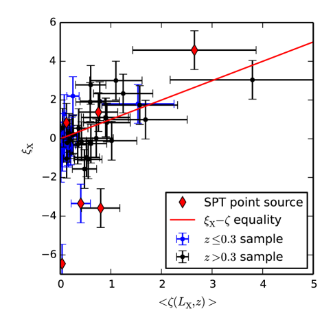
Figure 4: The measured significance $\xi_{\text{X}}$ versus the expected SPT-SZ $\langle\zeta(L_{\text{X}},z)\rangle$, where the best-fitting relation from the SPT-NPS sample and sampling bias corrections are applied. Overplotted is the line of equality. Clusters close to SPT point sources are marked with red diamonds.

Table 3: Constraints on the SZE $\zeta$-mass relation parameters.

	$A_{\text{SZ}}$	$B_{\text{SZ}}$
SPT High Mass (B13)	$1.50\pm 0.34$	$1.40\pm 0.16$
Prior	$[0.1-5]$	$[0.1-6]$
Full sample	$1.38^{+0.46}_{-0.36}$	$2.80^{+0.66}_{-0.63}$
SPT-NPS	$1.37^{+0.48}_{-0.38}$	$2.14^{+0.86}_{-0.66}$
SPT-NPS ($z>0.3$)	$1.37^{+0.60}_{-0.46}$	$2.31^{+1.31}_{-0.86}$
SPT-No-SUMSS	$1.42^{+0.58}_{-0.43}$	$2.14^{+0.91}_{-0.71}$

All three low mass subsamples show similar normalisation to the extrapolated high mass SPT-SZ sample, but there is a preference for larger slopes. The SPT-NPS sample is the best for comparison to the SPT-SZ high mass sample used in B13; this is because the SPT point sources have been removed to mimic the SPT cluster catalog selection and because there is no measurable difference between the SPT-NPS samples with or without the redshift cut.

The fact that we find consistent results with or without a low-redshift cut may at first be surprising, given that analyses of the high-mass SPT-SZ cut all clusters below z=0.3. In the SPT-SZ high mass sample, the low redshift clusters are cut because the angular scales of these clusters begin to overlap the scales where there is significant CMB primary anisotropy, making extraction with the matched filter approach using two frequencies difficult. However the XMM-BCS clusters are low mass systems with corresponding $R_{\text{c}}$ less than 1 arcmin even at low redshift. So we are able to recover the same scaling relation with or without the low redshift clusters.

The fully marginalised posterior probability distributions for $B_{\text{SZ}}$ can be used to quantify consistency between the two datasets. We do this for any pair of the distributions $P_{i}\left(\theta\right)$ by first calculating the probability density distribution of the difference $\Delta\theta$:

$$P(\Delta\theta)=\int\mathrm{d}\theta P_{1}(\theta)P_{2}(\theta-\Delta\theta).$$ (18)

We then calculate the likelihood $p$ that the origin ($\Delta\theta=0$) lies within this distribution as

$$p=\int_{S}\mathrm{d}\Delta\theta\ P(\Delta\theta)$$ (19)

where $S$ is the space where $P(\Delta\theta)<P(\Delta\theta=0)$. We then convert this $p$ value to an equivalent $N$-$\sigma$ significance within a normal distribution.

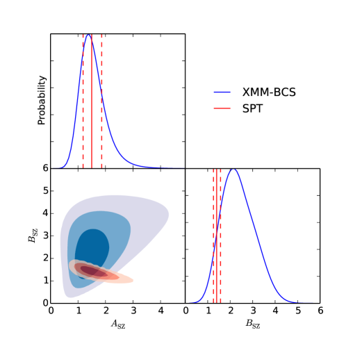
Figure 5: Constraints on the SPT-SZ $\zeta$-mass relation parameters $A_{\text{SZ}}$ and $B_{\text{SZ}}$ for the non-point source sample (SPT-NPS). The different shading indicates 1, 2, and 3$\sigma$ confidence regions. The constraints from the SPT-SZ high mass clusters (B13) are shown in red with 68 per cent confidence regions marked with dashed lines. The amplitudes for low and high mass clusters are compatible, but the slope is higher for low mass systems by about 1.4$\,\sigma$.

Overall, there is no strong statistical evidence that the low mass clusters behave differently than expected by simply extrapolating the high mass scaling relation to low mass; the slope parameter $B_{\text{SZ}}$ of the SPT-SZ high mass and SPT-NPS samples differs by only $1.4\,\sigma$ (tab:xbcs-constraint). The full sample has a $2.6\,\sigma$ higher $B_{\text{SZ}}$ than the SPT-SZ high mass sample (Benson et al., 2013). This steeper slope is presumably due to the contaminating effects of the SPT point sources. We find three outliers below the $L_{\text{X}}\text{-}\xi_{\text{X}}$ distribution (fig:xbcs-corrbias) that are all contaminated by SPT point sources. We list the separation between the cluster centres and the nearest SPT point source in tab:xbcs-cat.

It is clear from fig:xbcs-corrbias and from the results for the full sample that including X-ray-selected clusters that are associated with point sources that are independently detected in SPT-SZ data can bias the derived SZE-mass relation. In these cases, the affected clusters can be removed from the sample, and this particular bias can be easily avoided. Point sources that are not detected in the SPT-SZ data but which could be significantly affecting the measured SZE signal – particularly in low-mass clusters and groups – do remain a potential issue. We discuss this and the effect of point sources on our results more generally in sec:xbcs-PScontamination.

In addition to the X-ray bolometric luminosities, we test the luminosities based on two other bands (0.5–2.0 keV and 0.1–2.4 keV) as predictors of the cluster mass. After applying the appropriate $L_{\text{X}}$-mass relations listed in tab:xbcs-lxm we find that the changes to the parameter estimates are small. The largest change is on the slope of the SPT-SZ $\zeta$-mass relation, but the difference is less than $0.2\,\sigma$. Thus, the choice of X-ray luminosity band is not important to our analysis.

Our results show some dependence on the assumed $L_{\text{X}}$-mass scaling relation. Adopting the Vikhlinin et al. (2009) scaling relation has no significant impact on our results. However, with the Mantz et al. (2010a) $L_{\text{X}}$-mass relation, the slope decreases to $B_{\text{SZ}}\sim 1.57$ from 2.14, which makes the SPT-NPS sample almost a perfect match to the high mass SPT-SZ scaling relation. This shift is not surprising, because the Mantz et al. (2010a) $L_{\text{X}}$-mass relation has a very different slope from Pratt et al. (2009) (1.63 vs. 2.08, respectively). This causes clusters with a $L_{\text{X}}<1\times 10^{44}~{}\mathrm{erg\ s}^{-1}$to have significantly lower estimated masses when assuming the Mantz et al. (2010a) relation (20 per cent on average and $\sim 40$ per cent at the low mass end). We expect the Pratt et al. (2009) relation to be more appropriate for our analysis, because the Mantz et al. (2010a) relation was calibrated from higher mass clusters, using only clusters with $L_{\text{X}}>2.5\times 10^{44}~{}\mathrm{erg\ s}^{-1}$, above the majority of XMM-BCS clusters. Also we note the change of $\xi_{\text{X}}$ caused by the updated $R_{\text{500c}}(L_{\text{X}})$ is negligible, which has been shown also in Saliwanchik et al. (2013).

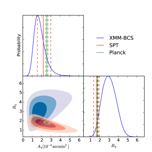
Figure 6: Constraints on the $Y_{\text{500}}$-mass relation parameters $A_{\text{Y}}$ and $B_{\text{Y}}$ for the non-point source sample (SPT-NPS). The SPT-NPS constraints are shown in blue and different shades show the 1, 2, and 3 $\sigma$ levels. The red is for the SPT-SZ result (Andersson et al., 2011), and the green is the best fit from the Planck analysis (P11). Marginalised constraints for each parameter are shown in blue with best fit and $1\,\sigma$ confidence regions marked by solid and dashed lines, respectively.

4.4 SZE $Y_{\text{500}}$-mass Relation

We measure the $Y_{\text{500}}$-mass relation, using the SPT-NPS sample. A similar fitting approach is used to account for the selection bias and with the same shifted pivot mass in eq:xbcs-ym of $1.5\times 10^{14}~{}\mathrm{M_{\odot}}$. The best fit parameters and uncertainties are presented in tab:xbcs-yszm along with the results from Andersson et al. (2011) and P11, which are adjusted to use our lower pivot mass. The $Y_{\text{500}}$ is based on the Arnaud profile and the $L_{\text{X}}$ is based on the X-ray luminosity measured within the 0.1–2.4 keV band, which facilitates the comparison with the P11 result. The impact from different profiles is discussed later in this section.

fig:xbcs-ym shows the joint parameter and fully marginalised constraints for $A_{\text{Y}}$ and $B_{\text{Y}}$. The shaded regions denote the 1, 2, and 3 $\sigma$ confidence regions as in fig:xbcs-AszBsz with blue for the SPT-NPS, red for the SPT-SZ sample Andersson et al. (2011), and green for the Planck sample (P11). This figure shows that the low mass SPT-NPS sample has rather weak constraints that are shifted with respect to the high mass SPT-SZ sample and the Planck sample.

We estimate the significance of the difference using the method described in sec:xbcs-xim. We quantify the consistency between any pair of the two-parameter distributions $P_{i}\left(\bm{\theta}\right)$ by calculating a $p$ value in a manner similar to that in eq:xbcs-1dp2exceed with the null hypothesis $\Delta\bm{\theta}=0$. Using this approach, we calculate that the SPT-NPS sample is roughly consistent with the high mass SPT-SZ sample (a $1.4\,\sigma$ difference) but is in tension with the Planck result (a $2.8\,\sigma$ difference).

Also shown in fig:xbcs-ym are the fully marginalised single parameter constraints. These distributions indicate that the normalisation differs by $0.8\sigma$ ($1.6\,\sigma$), and the slope parameter differs by $1.7\,\sigma$ ($1.7\,\sigma$) for the SPT-SZ (Planck) sample. Alternatively, we fix $B_{\text{Y}}=1.67$ ($1.78$) to limit the impact of the large uncertainty on the slope on the constraint of the normalisation. In this case, we find $A_{\text{Y}}=1.33^{+0.34}_{-0.31}$ ($1.37^{+0.36}_{-0.32}$) and the discrepancy on $A_{\text{Y}}$ is $1.5\,\sigma$ ($3.1\,\sigma$) for the SPT-SZ (Planck) sample. As in the $\zeta$-mass relation, there is no strong statistical evidence that the SPT-SZ clusters at low mass behave differently than those at high mass. Tighter constraints on the high mass SPT-SZ scaling relation will be helpful to understand the tension.

The tension with the Planck sample is intriguing; here we discuss several possible issues that could contribute. One difference is in the mass ranges probed in the two studies. In P11, the Planck team studies the relation between X-ray and SZE properties of 1600 clusters from the Meta-Catalogue of X-ray detected Clusters of galaxies (MCXC, Piffaretti et al., 2011) that span two decades in luminosity ($10^{43}~{}\mathrm{erg\ s^{-1}}\lesssim L_{500,[0.1\ -\ 2.4~{}\mathrm{keV}]}E(z)^{-7/3}\lesssim 2\times 10^{45}~{}\mathrm{erg\ s^{-1}}$). In contrast, our sample spans the range $10^{42}\mathrm{erg\ s^{-1}}\lesssim L_{500,[0.1\ -\ 2.4~{}\mathrm{keV}]}E(z)^{-7/3}\lesssim 10^{44}~{}\mathrm{erg\ s^{-1}}$ extending into the galaxy group regime. Thus, it is interesting to probe for any mass trends in the discrepancy. In fig:xbcs-cmpplanck, we show our measurements along with the Planck relation with fixed slope and redshift evolution as listed in Table 4 in P11 (solid black line). At the luminous (massive) end, our sample matches well with the Planck result (cyan points are taken from Figure 4 in P11). Beyond the Planck sample at the faint end, we find the preference for lower $Y_{\text{500}}$ relative to the Planck relation.

In the Planck analysis, an $L_{\text{X}}$-mass relation without Malmquist bias correction is used (Pratt et al., 2009). They argue that based on the similarity between the REXCESS and MCXC samples, there is no bias correction needed. In our analysis, we use the Malmquist bias-corrected relation and our likelihood corrects for selection bias. Using the non-corrected relation (Pratt et al., 2009) has very little impact. Interestingly, if we adopt the Mantz et al. (2010a) relation, the tension between our result and the Planck result disappears mainly due to the lower masses predicted by the relation as discussed in sec:xbcs-xim. However, given that the Planck analysis adopted the Pratt et al. (2009) relation, it is with this same relation that the most meaningful comparisons can be made.

Table 4: Constraints on the $Y_{\text{500}}$-mass relation.

Parameter	$A_{\text{Y}}[10^{-4}\mathrm{arcmin^{2}]}$	$B_{\text{Y}}$
SPT-NPS	$1.59^{+0.63}_{-0.48}$	$2.94^{+0.77}_{-0.74}$
SPT-No-SUMSS	$1.72^{+1.01}_{-0.66}$	$3.29^{+0.84}_{-0.96}$
SPT	$2.19\pm 0.63$	$1.67\pm 0.29$
Planck	$2.57\pm 0.11$	$1.78\pm 0.05$

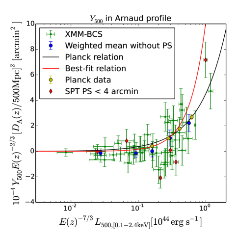
Figure 7: Comparison with the Planck $Y_{\text{500}}-L_{\text{X}}$ relation. The green dots are XMM-BCS clusters with $1\,\sigma$ uncertainty on $\xi_{\text{X}}$ and measured uncertainties on $L_{\text{X}}$ converted from the 0.5–2 keV band. Blue points are inverse variance weighted means of ensembles of the XMM-BCS sample. The black line is the Planck SZE relation from table 4 in P11 with the last four binned data points from figure 4 (P11) in cyan. The red line is the best-fit relation from the SPT sample. The correction of selection bias leads to a higher-than-measured $Y_{\text{500}}$ at high mass (luminous) end as the mass function is steep.) Consistent with our parameter constraints in fig:xbcs-ym, our measurements prefer a lower value than the Planck relation. Clusters close to SPT point sources are marked with red diamonds.

Second, the Planck relation is dominated by the high mass clusters, and their measurements at the low luminosity end (marked by cyan points in fig:xbcs-cmpplanck) also tend to fall below their best fit relation. The lowest luminosity Planck point has a $Y_{\text{500}}$ that is 68 per cent (2 $\sigma$ offset) of the value of the best fit model at the same X-ray luminosity. Interestingly, the best fit normalisation of the SPT-NPS sample is 53 per cent of the Planck model normalisation. In this sense, the tension between the two low mass samples is less than the tension between our sample and the best-fitting Planck relation.

Third, we note the redshift dependence of $Y_{\text{500}}$-mass relation could lead to a different normalisation because the SPT-XBCS sample is on average at higher redshift than the Planck sample. In P11, they show a weak redshift evolution of $Y_{\text{500}}$, where the index of $E(z)$ term is $-0.007\pm 0.518$. When they fit with the redshift evolution fixed to the self-similar expectation ($2/3$), it changes the $Y_{\text{500}}$ normalisation by $-5$ per cent ($0.451/0.476$), because $E(z)$ is larger than 1 for $z>0$. In comparison, if we assume an index of 0 for $E(z)$ it will increase our $Y_{\text{500}}$ normalisation by 19 per cent compared to the $E(z)^{2/3}$ case (XMM-BCS sample has a mean redshift of $0.48$). In this sense, there is some systematic uncertainty in the tension between the two samples that depends on the true redshift evolution of the $Y_{\text{500}}$-mass relation. If the samples evolve self-similarly, then the Planck normalisation should be reduced by 5 per cent.

Finally, the comparison to Planck is complicated because of differences between the SPT and Planck instruments and datasets and also differences between the analyses. Our analysis of SPT-SZ data calculates the SZE signal exclusively at frequencies below the SZE null (95 GHz and 150 GHz), where the SZE signal is negative, while Planck also includes information from frequencies above the 220 GHz SZE null, where the signal is positive. Thus, contamination from sources like radio galaxies with steeply falling spectra, which primarily affect the lowest-frequency bands in both instruments, would tend to bias both the Planck and SPT-SZ relations in the same way. But there are other possible sources of contamination such as dusty star-forming galaxies that are much brighter at higher frequencies. A population of star-forming galaxies associated with clusters could artificially increase the Planck measured $Y_{\text{500}}$, but could only negatively bias the SPT-SZ measurements. In their paper, the Planck team shows that at the low mass end (stellar mass smaller than $10^{11.25}\mathrm{M_{\odot}}$), the $Y_{\text{500}}$ estimated by six high frequency bands directly is higher than the $Y_{\text{500}}$ estimated when using a thermal dust model and the $Y_{\text{500}}$ estimated just using the three low frequencies (100, 143, 217 GHz) (Planck Collaboration ., 2013c). However, at higher masses where we are seeing the discrepany between the SPT and Planck signals there is no clear evidence for a dust related systematic in the cross-checks carried out by the Planck team. We present 2.8$\sigma$ significant evidence for dusty galaxy flux in our cluster ensemble in sec:xbcs-PScontamination below. If present, this flux is likely contributing to some degree to the discrepancy we find between the SPT and Planck SZE signatures on these mass scales.

In summary, there are several potential contributing factors to the 2.8$\sigma$ tension between the two results. None of them provide a convincing explanation for the offset on their own, but there are indications that differential sensitivity to dusty galaxy flux in SPT and Planck could be playing a role. What is needed next is a larger sample with higher quality data to probe this tension and – if the tension persists – to provide insights into the underlying causes of the discrepancy.

4.5 Potential Systematics

In the likelihood approach, we fix the cosmological parameters and assume no redshift uncertainty to improve the efficiency of the calculation. We test both of these assumptions and find that neither significantly impacts the analysis. Specifically, the mass function used for correcting the sampling bias is adopted from a fixed cosmology $(\Omega_{\mathrm{M}},\Omega_{\Lambda},H_{0})=(0.3,0.7,70~{}\text{km s}^{-1}\text{Mpc}^{-1})$. When we alter these to the recent WMAP results for $\Lambda$CDM Komatsu et al. (2011), we find a negligible impact.

We test the importance of possible photometric redshift biases by shifting the redshifts of all clusters up (or down) by $1\,\sigma$. We update $L_{\text{X}}$ appropriately for the new redshifts, and we find a small ($0.5\,\sigma$) shift in the normalisation and no change to the slope. Therefore, redshift biases at this level would not significantly bias the analysis.

4.6 Point Source Population

As already noted (see Section 4.3), there is a tendency for the systems with the most negative $\xi_{\text{X}}$ to be those with nearby SPT point sources (see fig:xbcs-corrbias). In this section, we explore this association in more detail, testing whether it is biasing our constraints on the SZE mass–observable relations. For the purposes of our analysis, an object is identified as an SPT point source if it appears as a 4$\,\sigma$ detection in a single frequency point-source filtered SPT-SZ map in any of the three bands (95, 150, or 220 GHz). An area within a 4 arcmin radius around each point source is defined, and all X-ray selected clusters within that region are flagged. There are six clusters flagged in our sample, and these are denoted with red diamonds in the figures presented above. Given the number densities of the SPT point sources (6 deg^-2 in this field) and the X-ray selected clusters together with the association radius, we estimate a 36 per cent chance that these point sources are random associations with the clusters.

If we consider a smaller 2 arcmin association radius between the X-ray centre and the SPT point source location, we still find four associations: three of which correspond to the most negative $\xi_{\text{X}}$ in fig:xbcs-corrbias, and the fourth is detected only at 220 GHz by SPT (and therefore is likely a dusty galaxy). With the smaller association radius the probability of a random association drops to 7 per cent, providing $\sim 2\,\sigma$ evidence that these point sources are physically associated with the X-ray selected groups.

To further study the point source issue, we cross-match our cluster sample with radio sources detected at 843 MHz by the SUMSS. The survey covers the whole sky at $\delta\leq-30^{\circ}$ with $|b|>10^{\circ}$ down to limiting source brightness of 6 mJy beam^-1. For the cross-matching, we utilise the latest version 2.1 of the catalog and a similar matching radius of 2 arcmin. This threshold is much larger than the SUMSS positional uncertainty, which has a median value of $\sim 2.3$ arcsec.

Within 2 arcmin of the X-ray centres, we find a total of 19 SUMSS point sources matching 18 clusters from our sample. In comparison, given the number density of SUMSS sources ($31.6$ deg^-2, Mauch et al., 2003), the number density of our clusters, and our association radius, we would expect to find $\sim 5$ clusters randomly overlapping with point sources in the $6~{}\text{deg}^{2}$ survey; there is a $3\times 10^{-4}$ per cent chance of explaining the associations as random superpositions. Thus, our small sample provides clear evidence of physical associations between low frequency radio point sources and X-ray selected groups and clusters; this is consistent with previous findings Best et al. (2005); Lin & Mohr (2007) that low frequency radio sources are associated with cluster galaxies in both optically and X-ray selected cluster samples. As expected, given the tendency for radio galaxies to have steeply falling spectra as a function of frequency, only a small fraction (3 out of 19) of these low frequency radio galaxies are detectable at SPT frequencies.

We use the BCS data (Desai et al., 2012) to examine the optical counterparts of the six SPT point sources that lie within 4 arcmin of our X-ray selected group and cluster sample. We do this by first associating the SPT point sources with a SUMSS source, which in general is only possible for the radio galaxies and not the dusty galaxies (Vieira et al., 2010). For our sample, three of the SPT point sources within 4 arcmin of the X-ray selected groups and clusters have SUMSS counterparts. All three of these have strongly negative $\xi_{\text{X}}$ (see fig:xbcs-corrbias). For two of the three point sources, the optical counterpart is the group BCG. In the third case the SPT point source corresponds to a quasar candidate (MRC 2319-550; Wright & Otrupcek, 1990) and does not appear to be a cluster member. The three remaining SPT point sources do not have SUMSS counterparts and are likely dusty galaxies; the SZE signatures $\xi_{\text{X}}$ of those systems are not obviously impacted. Thus we confirm that in two of our 46 low mass systems there are associated radio galaxies bright enough to be detected at SPT frequencies.

Based on the prediction from Lin et al. (2009), we would have expected that radio sources completely fill in the $Y_{\mathrm{SZ}}$ signal (100 per cent contamination) at a redshift of 0.1 (or a redshift of 0.6) in approximately 2.5 (or 0.5) percent of clusters with similar mass ($M_{200}=10^{14}\mathrm{M_{\odot}}$). For our 46 cluster sample, we would have expected this to happen for 1.15 (or 0.23) clusters, consistent with the two clusters we find associated with radio galaxies detected as point sources by SPT-SZ. We also expect a 20 per cent level $Y_{\text{SZ}}$ contamination on 9 (2) per cent of the sample. This predicted contamination is significantly smaller than our current uncertainties on the $Y_{\mathrm{SZ}}$ normalisation, and therefore cannot be tested in this analysis.

We repeat the SZE-mass relation analysis while excluding the half of the clusters with SUMSS point source associations. We find that the results are qualitatively similar using either the SPT-NPS or SPT-No-SUMSS sample (see Tables 3 and 4), although the uncertainties increase; this is consistent with the expectation that the level of the effect is too small to be measured with our sample. As already shown in Tables 3 and 4, our analysis shows no statistically significant difference in the SZE-mass relations when excluding or including the systems with nearby SPT point sources.

As pointed out in sec:xbcs-yszm, the dusty star-forming galaxies would have a net negative biasing impact on the SPT-SZ measurement. We examine the contamination from the dusty galaxies, which are not bright enough to be directly detectable in the 150 GHz and 95 GHz bands. To do this we measure the specific intensities at 220 GHz in a single frequency adaptive filter that uses cluster profiles at the locations of our X-ray selected cluster sample. In the SPT-NPS sample, the evidence for dusty galaxies is significant at the 2.8 $\sigma$ level. We then convert the 220 GHz intensities to temperature fluctuations at 150 GHz and 95 GHz by assuming the intensity follows $I\propto\nu^{3.6}$ for dusty sources Shirokoff et al. (2011). These are then converted to the corresponding values of $Y_{\text{500}}$. Dividing then by the expected $Y_{\text{500}}$ for a cluster of this redshift and X-ray luminosity, we then estimate the inverse variance weighted mean contamination to be $32\pm 18$ per cent and $7\pm 4$ per cent at 150 GHz and 95 GHz, respectively. Together, this contamination would lead the SPT-SZ observed $Y_{\text{500}}$ signature to be biased low by $\sim(17\pm 9)$ per cent. This fractional contamination depends on the mass and redshift of the cluster together with the typical star formation activity. In particular, as a function of mass the SZE signature grows as $Y_{\text{500}}\propto M^{5/3}$, whereas the blue or star forming component of the galaxy population falls (e.g. Weinmann et al., 2006); thus, contamination would fall with mass. As one pushes to even higher redshift than this sample (i.e. $z>1$) where star formation is more prevalent, the contamination would be expected to increase.

This level of contamination is consistent with a recent study of $\sim 550$ galaxy clusters selected via optical red-sequence techniques. Using Herschel and SPT mm-wave data to jointly fit an SZE+dust spectral model, Bleem (2013) finds the contamination at 150 GHz to be $40\pm 30$ per cent for low-richness optical groups ($M_{\textrm{200}}\sim 1\times 10^{14}\mathrm{M_{\odot}}$). The fractional contamination declines as a function of optical richness and is measured to be $5\pm 5$ per cent for the richest 3 per cent of clusters in the sample sample ($M_{\textrm{200}}\sim 3\text{--}6\times 10^{14}\mathrm{M_{\odot}}$). A larger sample size combined with deeper mm-wave data will improve our ability to estimate the contamination from dusty galaxies in clusters and groups.

In summary, this small sample of 46 X-ray selected groups and low mass clusters provides high significance evidence of having physically associated low frequency SUMSS radio galaxies. For the SPT point source sample within 2 arcmin, there is less than $2\,\sigma$ statistical evidence of physical association, but two of the sources have optical counterparts that are in the groups. Although we would expect physically associated high frequency radio galaxies to bias the SZE mass-observable relation, our analysis provides no evidence of this impact. We use the 220 GHz SPT-SZ data in this sample to estimate that the $Y_{\text{500}}$ measured by the SPT is biased $\sim 17\pm 9$ per cent low. A larger sample from a broader survey (through XMM-XXL or eROSITA, for example) or a deeper SZE survey would both help to improve our understanding of the impact of point sources.

5 Conclusions

Using data from the SPT-SZ survey, we have explored the SZE signatures of low mass clusters and groups selected from a uniform XMM-Newton X-ray survey. The cluster and group sample from the XMM-BCS has a well understood selection, and previously published calibrations of the $L_{\text{X}}$-mass relation allow us to estimate the masses of each of these systems. Although these systems have masses that are too low for them to have been individually detected within the SPT-SZ survey, we are able to use the ensemble to constrain the underlying relationship between the halo mass and the SZE signature for low mass systems.

Our method corrects for the Eddington bias and shows that there is no Malmquist like bias effect on the SZE mass-observable relation within this X-ray selected sample. We test our likelihood using a large mock sample, and we show with the current sample size we can at most extract constraints from two scaling relation parameters: the power law amplitude $A_{\text{SZ}}$ and slope $B_{\text{SZ}}$ (see Equations 5 and 12).

We separate the sample of 46 groups and clusters into three subsamples: (1) the full sample, (2) the point source-free sample, for which we exclude systems with point sources detected at significance $>$4 at either 95, 150, or 220 GHz in the SPT-SZ data within 4 arcmin radius of the X-ray centre, and (3) the point source-free sample, with clusters at $z<0.3$ excluded. We find that, due to the point source contamination in three of the lowest $\xi_{\text{X}}$ groups, the full sample exhibits a steep slope ($B_{\text{SZ}}=2.80^{+0.66}_{-0.63}$) that is in tension at 2.6$\,\sigma$ with the high mass SPT sample ($B_{\text{SZ}}=1.40\pm 0.16$). The point source free subsample has a slope ($B_{\text{SZ}}=2.14^{+0.86}_{-0.66}$) that is in rough agreement with the slope of the high mass SPT sample ($1.4\sigma$ difference). We find no evidence that the low redshift clusters deviate from the scaling relation of the point source free sample.

We also measure the $Y_{\text{500}}$-mass relation for our sample and compare it to the results from the SPT-SZ high mass clusters and the Planck sample. Our low mass sample exhibits a preference for lower normalisation and steeper slope than the other two samples, but the uncertainties are large (see fig:xbcs-ym and tab:xbcs-yszm). Within the SPT samples, there is no statistically significant evidence for differences in the scaling relation as one moves from high to low masses. On the other hand, the Planck sample exhibits a 2.8 $\sigma$ significant tension with our sample. As shown in fig:xbcs-cmpplanck, the lowest X-ray luminosity portion of our sample has lower $Y_{\text{500}}$ than expected from the Planck relation. We discuss a range of possible explanations for this tension (Section 4.4), in particular contamination from dusty sources. Given the significance level of the tension the appropriate next step is to enlarge the sample to better quantify the differences in the SZE signatures of low and high mass clusters and the possible differences between Planck and SPT.

We examine radio point source contamination. Cross-matching our X-ray selected groups and clusters with the SUMSS catalog, we find that 18 of 46 members have associated 843 MHz SUMSS point sources within 2 arcmin. This represents highly significant evidence of physical association between our sample and low frequency point sources. At higher frequencies, we find four systems with associated SPT detected point sources; three of these also have SUMSS counterparts. Two of these three point sources have optical counterparts that lie within the X-ray group, and the third is a quasar candidate that is likely unassociated with the group. Having two out of 46 groups or clusters with physically associated bright, high frequency point sources is consistent with the expectations from Lin et al. (2009). The predicted contamination from undetected radio point sources (Lin & Mohr, 2007; Lin et al., 2009) in the remainder of the sample is significantly smaller than our measurement uncertainty on the $Y_{\text{500}}$ normalisation, and so we cannot test these predictions here.

We also examine the impact of undetected dusty galaxies. Using the SPT-SZ 220 GHz band, we find 2.8$\,\sigma$ significant evidence of a flux excess due to dusty galaxies. Extrapolating to lower frequencies, we estimate that the measured $Y_{\text{500}}$ signature is biased low by $\sim(17\pm 9)$ per cent in this ensemble of low mass clusters and groups. Given the different frequency coverage of Planck and SPT, it is not clear that the Planck bias due to dusty galaxy flux would be the same. If flux from dusty galaxies would induce a smaller negative bias or even a positive bias in Planck $Y_{\text{500}}$ measurements, then that would reduce the tension between the Planck $Y_{\text{500}}$–mass relation and ours.

We point out that these contamination levels are for this X-ray selected low mass sample with a median mass of $10^{14}\mathrm{M_{\odot}}$, which is significantly below the typical mass of SPT selected clusters. Given the increasing rarity of blue and star forming galaxies as one moves from groups to high mass clusters (e.g Weinmann et al., 2006), any contamination in the SPT selected sample would be much lower.

Finally, the receiver on the SPT was upgraded in 2012. The SPTpol camera provides sensitivity to CMB polarization and, more importantly for SZE work, increased sensitivity to CMB temperature fluctuations. The final SPTpol maps are expected to cover 500 square degrees of sky to noise levels of $\sim 5$ and $\sim 9\mathrm{\mu K-arcmin}$ at 150 and 95 GHz (Austermann et al., 2012). Meanwhile, the XXL survey Pierre et al. (2011) has increased the survey area that has a characteristic 10 ks XMM-Newton exposure from $6~{}\text{deg}^{2}$ to $25~{}\text{deg}^{2}$. This should enable an interesting new insight into possible differences in the SZE signatures of low and high mass clusters. We make a forecast with a mock catalog that consists of 144 clusters within redshift range 0.2–1.2 and a bolometric flux limit of $1\times 10^{-14}~{}\text{erg s}^{-1}\text{cm}^{-2}$. Analysing this sample with the appropriate SPTpol increase in depth indicates that with the future sample we can tighten the fractional error on $A_{\text{SZ}}$ to 6 per cent compared to our current result of 30 per cent. On $B_{\text{SZ}}$ the uncertainty shrinks from 34 to 8 per cent. These improvements should enable a more revealing comparison of the SZE signatures of low and high mass clusters and perhaps also enable a detailed study of potential contamination of the SZE signal by associated radio or dusty galaxies.

Appendix A Likelihood function

We start from the full likelihood function based on B13 to constrain both the cosmological model and the scaling relations as (note that the observables are different from the ones used in B13):

$$\ln\ \mathcal{L}(\bm{c},\bm{r}_{\text{SZ}},\bm{r}_{\text{X}},\Theta) =\sum_{i}\ln\frac{\mathrm{d}N(Y_{i},f_{i},z_{i}|\bm{c},\bm{r}_{\text{SZ}},\bm{r}_{\text{X}},\Theta)}{\mathrm{d}Y\mathrm{d}f\mathrm{d}z}$$

$$-\iiint\frac{\mathrm{d}N(Y,f,z|\bm{c},\bm{r}_{\text{SZ}},\bm{r}_{\text{X}},\Theta)}{\mathrm{d}Y\mathrm{d}f\mathrm{d}z}\mathrm{d}Y\mathrm{d}f\mathrm{d}z,$$ (20)

where $i$ runs over the cluster sample, $Y_{i}$ is the SZE signal (i.e. $\xi_{\text{X}}$ or $Y_{\text{500}}$), $f_{i}$ is the X-ray flux, and $z_{i}$ is the redshift. $\bm{r}_{\text{SZ}}$ represents the SZE scaling relation, $\bm{r}_{\text{X}}$ represents the X-ray scaling relation, and $\Theta$ describes the sample selection. $\mathrm{d}N(Y_{i},f_{i},z_{i}|\bm{c},\bm{r}_{\text{SZ}},\bm{r}_{\text{X}},\Theta)$ is the expected number of clusters within a three-dimensional cell $\mathrm{d}Y\mathrm{d}f\mathrm{d}z$, and the second term is the integral of the differential cluster number density over all $Y$, $f$ and $z$.

Given the limited sample size, we focus on the SZE-mass scaling relation, keeping the cosmological $\bm{c}$ and the X-ray scaling relation $\bm{r}_{\text{X}}$ fixed. In addition, we assume the redshift measurements have insignificant uncertainties. Within this context, the X-ray flux is equivalent to the X-ray luminosity $L$.

The differential number density of clusters can be expressed as:

$$\frac{\mathrm{d}N(Y,L,z|\bm{c},\bm{r}_{\text{SZ}},\bm{r}_{\text{X}},\Theta)}{\mathrm{d}Y\mathrm{d}L\mathrm{d}z}$$

$$\ \ \ \ \ =P(Y|L,z,\bm{c},\bm{r}_{\text{SZ}},\bm{r}_{\text{X}},\Theta)\,\frac{\mathrm{d}N(L,z|\bm{c},\bm{r}_{\text{SZ}},\bm{r}_{\text{X}},\Theta)}{\mathrm{d}L\mathrm{d}z},$$ (21)

where the first factor is the conditional probability of $Y$ given observables $L$ and $z$ with other model parameters, and we are using the relation $\mathrm{d}N/\mathrm{d}Y=P(Y)N$. The second factor is the differential number density of clusters as a function of $L$ and $z$.

The full likelihood can be split into three parts:

$$\ln\mathcal{L}(\bm{c},\bm{r}_{\text{SZ}},\bm{r}_{\text{X}},\Theta)= \sum_{i}\ln P(Y_{i}|L_{i},z_{i},\bm{c},\bm{r}_{\text{SZ}},\bm{r}_{\text{X}},\Theta)$$

$$+ \sum_{i}\ln\frac{\mathrm{d}N(L_{i},z_{i}|\bm{c},\bm{r}_{\text{SZ}},\bm{r}_{\text{X}},\Theta)}{\mathrm{d}L\mathrm{d}z}$$

$$- \iiint\frac{\mathrm{d}N(Y,L,z|\bm{c},\bm{r}_{\text{SZ}},\bm{r}_{\text{X}},\Theta)}{\mathrm{d}Y\mathrm{d}L\mathrm{d}z}\mathrm{d}Y\mathrm{d}L\mathrm{d}z.$$ (22)

If the sample selection is based on the X-ray only, then we have:

$$\mathrm{d}N\left(L_{i},z_{i}|\bm{c},\bm{r}_{\text{SZ}},\bm{r}_{\text{X}},\Theta_{\text{X}}\right)=\Theta_{\text{X}}(L_{i},z_{i})\mathrm{d}N(L_{i},z_{i}|\bm{c},\bm{r}_{\text{X}}),$$ (23)

where $\Theta_{\text{X}}$ is simply the probability that a cluster with X-ray luminosity $L_{i}$ and redshift $z_{i}$ is observed. In addition,

$$\int P(Y|L,z,\bm{c},\bm{r}_{\text{SZ}},\bm{r}_{\text{X}},\Theta_{\text{X}})\mathrm{d}Y=1,$$ (24)

which simply means that, because there is only X-ray selection $\Theta_{\text{X}}$, any cluster that makes it into the sample due to its X-ray properties will always have a corresponding value $Y$. Using this condition together with eq:xbcs-conditional-yl allows us to write the third term in eq:full-likelihood-3 as:

$$\iiint\frac{\mathrm{d}N(Y,L,z|\bm{c},\bm{r}_{\text{SZ}},\bm{r}_{\text{X}},\Theta_{\text{X}})}{\mathrm{d}Y\mathrm{d}L\mathrm{d}z}\mathrm{d}Y\mathrm{d}L\mathrm{d}z$$

$$=\iint\frac{\mathrm{d}N(L,z|\bm{c},\bm{r}_{\text{X}},\Theta_{\text{X}})}{\mathrm{d}L\mathrm{d}z}\mathrm{d}L\mathrm{d}z.$$ (25)

Note that by adopting Equations (23) and (A), the last two terms in eq:full-likelihood-3 have no remaining dependence on $Y$ and depend only on cosmology $\bm{c}$, the X-ray-mass scaling relation $\bm{r}_{\text{X}}$ and the X-ray sensitive selection $\Theta_{\text{X}}$. Thus, within the context of a fixed cosmology and X-ray scaling relation these two terms are constant and do not contribute to constraining the SZE scaling relation $\bm{r}_{\text{SZ}}$. Thus, for the final likelihood that we use in this analysis, we obtain

$$\ln\mathcal{L}(\bm{r}_{\text{SZ}})=\sum_{i}\ln P(Y_{i}|L_{i},z_{i},\bm{c},\bm{r}_{\text{X}},\bm{r}_{\text{SZ}},\Theta_{\text{X}}).$$ (26)

The derivation of the likelihood is correct even in the presence of correlated scatter between $L$ and $Y$.

However if the selection were based on both $L$ and $Y$, then eq:xbcs-final-likelihood would no longer be equivalent to the full likelihood. For instance eq:xbcs-selection-x would need to be extended as:

$$\mathrm{d}N\left(L_{i},z_{i}|\bm{c},\bm{r}_{\text{SZ}},\bm{r}_{\text{X}},\Theta\right)=\int\mathrm{d}Y\Theta(Y,L_{i},z_{i})\mathrm{d}N(Y,L_{i},z_{i}|\bm{c},\bm{r}_{\text{X}},\bm{r}_{\text{SZ}}).$$ (27)

And therefore detailed modelling of the selection would be required to calculate the likelihood and constrain the scaling relation parameters.

References

- Allen et al. (2011) Allen S. W., Evrard A. E., Mantz A. B., 2011, ARAA, 49, 409
- Andersson et al. (2011) Andersson K. et al., 2011, ApJ, 738, 48
- Andersson et al. (2011) Andersson K. et al., 2011, ApJ, 738, 48
- Arnaud et al. (2010) Arnaud M., Pratt G. W., Piffaretti R., Böhringer H., Croston J. H., Pointecouteau E., 2010, A&A, 517, A92
- Austermann et al. (2012) Austermann J. E. et al., 2012, in SPIE Conf. Ser. Vol. 8452, Society of Photo-Optical Instrumentation Engineers (SPIE) Conference Series, p. 84521E
- Benson et al. (2013) Benson B. A. et al., 2013, ApJ, 763, 147
- Best et al. (2005) Best P. N., Kauffmann G., Heckman T. M., Brinchmann J., Charlot S., Ivezić Ž., White S. D. M., 2005, MNRAS, 362, 25
- Bleem (2013) Bleem L. E., 2013, PhD thesis, The University of Chicago
- Bock et al. (1999) Bock D. C.-J., Large M. I., Sadler E. M., 1999, AJ, 117, 1578
- Bocquet et al. (2014) Bocquet S. et al., 2014, preprint, (arXiv:1407.2942)
- Carlstrom et al. (2011) Carlstrom J. E. et al., 2011, PASP, 123, 568
- Cavaliere & Fusco-Femiano (1976) Cavaliere A., Fusco-Femiano R., 1976, A&A, 49, 137
- Desai et al. (2012) Desai S. et al., 2012, ApJ, 757, 83
- Fowler et al. (2007) Fowler J. W. et al., 2007, Applied Optics, 46, 3444
- Hasselfield et al. (2013) Hasselfield M. et al., 2013, JCAP, 7, 8
- Komatsu et al. (2011) Komatsu E. et al., 2011, ApJS, 192, 18
- Laganá et al. (2013) Laganá T. F., Martinet N., Durret F., Lima Neto G. B., Maughan B., Zhang Y.-Y., 2013, A&A, 555, A66
- Lin et al. (2009) Lin Y., Partridge B., Pober J. C., Bouchefry K. E., Burke S., Klein J. N., Coish J. W., Huffenberger K. M., 2009, ApJ, 694, 992
- Lin & Mohr (2007) Lin Y.-T., Mohr J. J., 2007, ApJS, 170, 71
- Majumdar & Mohr (2004) Majumdar S., Mohr J. J., 2004, ApJ, 613, 41
- Mantz et al. (2010a) Mantz A., Allen S. W., Ebeling H., Rapetti D., Drlica-Wagner A., 2010a, MNRAS, 406, 1773
- Mantz et al. (2010b) Mantz A., Allen S. W., Rapetti D., Ebeling H., 2010b, MNRAS, 406, 1759
- Mauch et al. (2003) Mauch T., Murphy T., Buttery H. J., Curran J., Hunstead R. W., Piestrzynski B., Robertson J. G., Sadler E. M., 2003, MNRAS, 342, 1117
- McDonald et al. (2013) McDonald M. et al., 2013, ApJ, 774, 23
- Melin et al. (2006) Melin J.-B., Bartlett J. G., Delabrouille J., 2006, A&A, 459, 341
- Mohr et al. (1999) Mohr J. J., Mathiesen B., Evrard A. E., 1999, ApJ, 517, 627
- Molnar et al. (2012) Molnar S. M., Hearn N. C., Stadel J. G., 2012, ApJ, 748, 45
- Mortonson et al. (2011) Mortonson M. J., Hu W., Huterer D., 2011, Phys. Rev. D, 83, 023015
- Motl et al. (2005) Motl P. M., Hallman E. J., Burns J. O., Norman M. L., 2005, ApJ, 623, L63
- Nagai et al. (2007) Nagai D., Kravtsov A. V., Vikhlinin A., 2007, ApJ, 668, 1
- Pierre et al. (2011) Pierre M., Pacaud F., Juin J. B., Melin J. B., Valageas P., Clerc N., Corasaniti P. S., 2011, MNRAS, 414, 1732
- Piffaretti et al. (2011) Piffaretti R., Arnaud M., Pratt G. W., Pointecouteau E., Melin J.-B., 2011, A&A, 534, A109
- Plagge et al. (2010) Plagge T. et al., 2010, ApJ, 716, 1118
- Planck Collaboration (2011a) Planck Collaboration et al., 2011a, A&A, 536, A11
- Planck Collaboration (2011b) Planck Collaboration, 2011b, A&A, 536, A10
- Planck Collaboration (2013a) Planck Collaboration et al., 2013a, preprint, (arXiv:1303.5080)
- Planck Collaboration (2013b) Planck Collaboration et al., 2013b, preprint, (arXiv:1303.5076)
- Planck Collaboration . (2013c) Planck Collaboration et al., 2013c, A&A, 557, A52
- Pratt et al. (2009) Pratt G. W., Croston J. H., Arnaud M., Böhringer H., 2009, A&A, 498, 361
- Reichardt et al. (2013) Reichardt C. L. et al., 2013, ApJ, 763, 127
- Saliwanchik et al. (2013) Saliwanchik B. R. et al., 2013, preprint, (arXiv:1312.3015)
- Schaffer et al. (2011) Schaffer K. K. et al., 2011, ApJ, 743, 90
- Semler et al. (2012) Semler D. R. et al., 2012, ApJ, 761, 183
- Shirokoff et al. (2011) Shirokoff E. et al., 2011, ApJ, 736, 61
- Song et al. (2012a) Song J., Mohr J. J., Barkhouse W. A., Warren M. S., Rude C., 2012a, ApJ, 747, 58
- Song et al. (2012b) Song J. et al., 2012b, ApJ, 761, 22
- Stanek et al. (2006) Stanek R., Evrard A. E., Böhringer H., Schuecker P., Nord B., 2006, ApJ, 648, 956
- Story et al. (2013) Story K. T. et al., 2013, ApJ, 779, 86
- Sun et al. (2009) Sun M., Voit G. M., Donahue M., Jones C., Forman W., Vikhlinin A., 2009, ApJ, 693, 1142
- Sunyaev & Zel’dovich (1970) Sunyaev R. A., Zel’dovich Y. B., 1970, Comments on Astrophysics and Space Physics, 2, 66
- Sunyaev & Zel’dovich (1972) Sunyaev R. A., Zel’dovich Y. B., 1972, Comments on Astrophysics and Space Physics, 4, 173
- Tauber et al. (2010) Tauber J. A. et al., 2010, A&A, 520, A1
- Tinker et al. (2008) Tinker J., Kravtsov A. V., Klypin A., Abazajian K., Warren M., Yepes G., Gottlöber S., Holz D. E., 2008, ApJ, 688, 709
- Šuhada et al. (2012) Šuhada R. et al., 2012, A&A, 537, A39
- Vanderlinde et al. (2010) Vanderlinde K. et al., 2010, ApJ, 722, 1180
- Vieira et al. (2010) Vieira J. D. et al., 2010, ApJ, 719, 763
- Vikhlinin et al. (2009) Vikhlinin A. et al., 2009, ApJ, 692, 1033
- Weinmann et al. (2006) Weinmann S. M., van den Bosch F. C., Yang X., Mo H. J., 2006, MNRAS, 366, 2
- Williamson et al. (2011) Williamson R. et al., 2011, ApJ, 738, 139
- Wright & Otrupcek (1990) Parkes Catalogue, 1990, Australia Telescope National Facility, Wright & Otrupcek, (Eds)
- Zenteno et al. (2011) Zenteno A. et al., 2011, ApJ, 734, 3