Multiple positive solutions of parabolic systems with nonlinear, nonlocal initial conditions

Abstract.

In this paper we study the existence, localization and multiplicity of positive solutions for parabolic systems with nonlocal initial conditions. In order to do this, we extend an abstract theory that was recently developed by the authors jointly with Radu Precup, related to the existence of fixed points of nonlinear operators satisfying some upper and lower bounds. Our main tool is the Granas fixed point index theory. We also provide a non-existence result and some examples to illustrate our theory.

1. Introduction

In this paper we deal with the existence, non-existence and localization of positive solutions of the following system of parabolic equations subject to nonlinear, nonlocal initial conditions

(1.1) $$\begin{cases}u_{t}-\Delta u=f(t,x,u,v),&(t,x)\in(0,{t_{\text{max}}})\times\Omega,\\ v_{t}-\Delta v=g(t,x,u,v),&(t,x)\in(0,{t_{\text{max}}})\times\Omega,\\ u(t,x)=v(t,x)=0,&(t,x)\in(0,{t_{\text{max}}})\times\partial\Omega,\\ u(0,\cdot)=\alpha(u,v),\\ v(0,\cdot)=\beta(u,v),\end{cases}$$

where $\Omega\subset\mathbb{R}^{m}$ is a bounded Dirichlet regular domain (i.e. for all $\varphi\in C(\partial\Omega)$ there exists $u\in C(\overline{\Omega})$ such that $u|\partial\Omega=\varphi$ and $\Delta u=0$ in a distributional sense, see [1, Definition 6.1.1]), $f,g\colon(0,{t_{\text{max}}})\times\Omega\times\mathbb{R}_{+}\times\mathbb{R}_{+}\to\mathbb{R}_{+}$ are continuous functions and

(1.2) $$\alpha(u,v)=G_{1}\left(\int_{0}^{{t_{\text{max}}}}g_{1}(u(t),v(t))d\mu_{1}(t)\right),\quad\beta(u,v)=G_{2}\left(\int_{0}^{{t_{\text{max}}}}g_{2}(u(t),v(t))d\mu_{2}(t)\right),$$

where $g_{1},g_{2}\colon\mathbb{R}_{+}^{2}\to\mathbb{R}_{+}$, $G_{1},G_{2}\colon\mathbb{R}_{+}\to\mathbb{R}_{+}$ are continuous with $g_{i}(0,0)=G_{i}(0)=0$ for $i\in\{1,2\}$ and $\mu_{1},\mu_{2}$ are finite (positive) Borel measures on $[0,{t_{\text{max}}}]$ such that

$$\mu_{1}(\{0\})=\mu_{2}(\{0\})=0.$$

Note that the initial conditions (1.2) cover a variety of cases, a particular example being

(1.3) $$\alpha(u,v)(x)=\int_{0}^{{t_{\text{max}}}}u(t,x)dt,\quad\beta(u,v)(x)=\int_{0}^{{t_{\text{max}}}}v(t,x)dt.$$

Note that the system (1.1) can be applied to describe physical phenomena in which it is possible to measure the sums of amounts of substances according to formulae of the type (1.3) or

(1.4) $$\alpha(u,v)=\sum_{s=1}^{k}\alpha_{s}u(t_{s}),\quad\beta(u,v)=\sum_{s=1}^{r}\beta_{s}v(t^{\prime}_{s}),$$

where $0<t_{1}<\ldots<t_{k}$, $0<t^{\prime}_{1}<\ldots<t^{\prime}_{r}$ and $\alpha_{s},\beta_{s}>0$. For example, the system (1.1) with the nonlocal initial conditions (1.4) can be used to model a reaction-diffusion process of a little amount of gases in a transparent tube, in a more appropriate way than with the usual initial-value condition; for more insight on the physical interpretation of this system see the paper by Byszewski [3]. We mention that a physical motivation for the integral form of the initial condition is presented in [4, 5, 23]. Moreover, the system (1.1) can be used to describe the periodic solutions in the case $\alpha(u,v)=u(T)$, $\beta(u,v)=v(T)$, where $T>0$ and $f$ and $g$ are $T$-periodic. Furthermore, a number of applications of nonlocal problems for evolution equations are illustrated in Section 10.2 of [22].

Initial nonlocal conditions have been investigated in a variety of settings, for example in the case of multi-point [10], integral [9, 13, 23, 24, 26, 27] and nonlinear conditions [2, 6, 7, 8], see also the recent review [28].

In a recent paper [19] the authors investigated the existence, localization and multiplicity of positive solutions of systems of $(p,q)$-Laplacian equations subject to Dirichlet boundary conditions. The main tool in [19] is the development of a general abstract framework for the existence of fixed points of nonlinear operators acting on cones that satisfy an inequality of Harnack-type. Within this setting, the authors of [19] used the Granas fixed point index (see for example [12, 16]) and, in order to compute the index, they used some estimates from above, using the norm, and from below, utilizing a seminorm. Here we extend the theoretical results of [19] to a more general setting; this generalization is apparently simple but fruitful and is motivated by the application to the parabolic system (1.1). In particular, we replace the use of the seminorm with the use of a more general positively homogeneous functional and, moreover, we relax the assumptions on the cone. The Remarks 2.5, 3.6, and 3.17 illustrate in details the differences between the two theoretical approaches and their applicability. We point out that our new approach is quite general and covers, as a special case, the system (1.1).

The problem of one parabolic equation with nonlocal, linear initial condition was stated and discussed in [25]. By modifying the theoretical setting as described above, we overcome the difficulties arisen in [25], obtaining the results predicted by [25].

In contrast with the paper [19], where the space $L^{\infty}$ with an integral seminorm was used, here, in order to seek mild solutions of our problem, we use the classical space of continuous functions, with a very natural positively homogeneous functional, namely the minimum on a suitable subset. A similar idea has been used with success in the context of ordinary differential equations and integral equations, see for example [12, 17, 21]. In our case, a key role for our multiplicity results is played by a weak Harnack-type inequality, see Remark 3.9.

In the case of the system (1.1) we obtain existence, localization, multiplicity and non-existence of positive mild solutions.

We illustrate in two examples the applicability of our results and we show that the constants that occur in our theory can be computed.

2. Abstract existence theorems

In this Section we generalize the abstract results of Section 2 of [19]. Although these results are motivated by the solvability of the parabolic system (1.1), we present them in a greater generality, as we believe that they are of independent interest, since they can be applied in other contexts, whenever an abstract Harnack-type inequality is available.

For $i=1,2$, let $(E_{i},|\cdot|_{i})$ be a Banach space and let $\left\lfloor\cdot\right\rfloor_{i}$ be a given positively homogeneous continuous functional on $E_{i}$. In what follows, we omit the subscript in $\left\lfloor\cdot\right\rfloor_{i}$, when confusion is unlikely.

Let also $G_{i}\subset E_{i}$ be closed convex wedges, which is understood to mean that

$$\lambda u+\mu v\in G_{i}\text{ for all }u,v\in G_{i}\text{ and }\lambda,\mu\geq 0.$$

Moreover, let $K_{i}\subset G_{i}$ be closed convex cones, which means that $K_{i}$ are closed convex wedges such that $K_{i}\cap(-K_{i})=\{0\}$. The wedges induce the natural semiorders $\preceq$ on $E_{i}$ in the following way:

$$u\preceq v\ \text{if and only if}\ v-u\in G_{i},\,u,v\in E_{i}.$$

By a semiorder we mean that the relation $\preceq$ is reflexive and transitive, but not necessarily antisymmetric.

We assume that the functionals $\left\lfloor\cdot\right\rfloor_{i}$ are monotone on $K_{i}$ with respect to the semiorder $\preceq$, that is for $i\in\{1,2\}$ we have

(2.1) $$\text{if }u\preceq v\text{ then }\left\lfloor u\right\rfloor\leq\left\lfloor v\right\rfloor\text{ for }u,v\in K_{i}.$$

In particular we have $\left\lfloor u\right\rfloor\geq 0$ for $u\in K_{i}$.

We assume that there exist some elements $\psi_{i}\in K_{i}$ such that $|\psi_{i}|=1$ and for $i\in\{1,2\}$

(2.2) $$u\preceq|u|\psi_{i}\text{ for all }u\in K_{i}.$$

Note that (2.1) and (2.2) yield

(2.3) $$\left\lfloor u\right\rfloor_{i}\leq\left\lfloor\psi\right\rfloor|u|\text{ for all }u\in K_{i}.$$

In particular, we have $\left\lfloor\psi_{i}\right\rfloor>0$ if $\left\lfloor\cdot\right\rfloor$ is nonzero.

In what follows by the compactness of a continuous operator we mean the relative compactness of its range. By the complete continuity of a continuous operator we mean the relative compactness of the image of every bounded set of the domain.

We seek the fixed points of a completely continuous operator

$$N:=(N_{1},N_{2})\colon K_{1}\times K_{2}\to K_{1}\times K_{2},$$

that is $(u,v)\in K_{1}\times K_{2}$ such that $N(u,v)=(u,v)$.

We shall discuss not only the existence, but also the localization and multiplicity of the solutions of the nonlinear equation $N(u,v)=(u,v)$. In order to do this, we utilize the Granas fixed point index, $\mathrm{ind}_{C}(f,U)$, which roughly speaking, is the algebraic count of the fixed points of $f$ in the set $U$. The formal definition of the index involves the Leray-Schauder degree and retractions, for more information on the index and its applications we refer the reader to [12, 16].

The next Proposition describes some of the useful properties of the index, for details see Theorem 6.2, Chapter 12 of [16].

Proposition 2.1.

Let $C$ be a closed convex subset of a Banach space, $U\subset C$ be open in $C$ and $f\colon\overline{U}\rightarrow C$ be a compact map with no fixed points on the boundary $\partial U$ of $U.$ Then the fixed point index has the following properties:

(i) (Existence) If $\mathrm{ind}_{C}(f,U)\neq 0$ then $\mathrm{fix}(f)\neq\emptyset$, where $\mathrm{fix}f=\mbox{$\left\{x\in\bar{U}:\;f(x)=x\right\}$}$.

(ii) (Additivity) If $\mathrm{fix}f\subset U_{1}\cup U_{2}\subset U$ with $U_{1},U_{2}$ open in $C$ and disjoint, then

$$\mathrm{ind}_{C}(f,U)=\mathrm{ind}_{C}(f,U_{1})+\mathrm{ind}_{C}(f,U_{2}).$$

(iii) (Homotopy invariance) If $h\colon\overline{U}\times[0,1]\rightarrow C$ is a compact homotopy such that $h(u,t)\neq u$ for $u\in\partial U$ and $t\in[0,1]$ then

$$\mathrm{ind}_{C}(h(\cdot,0),U)=\mathrm{ind}_{C}(h(\cdot,1),U).$$

(iv) (Normalization) If $f$ is a constant map, with $f(u)=u_{0}$ for every $u\in\overline{U},$ then

$$\mathrm{ind}_{C}(f,U)=\begin{cases}1,\quad\text{if}\ u_{0}\in U\\ 0,\quad\text{if}\ u_{0}\notin\overline{U}.\end{cases}$$

In particular, $\mathrm{ind}_{C}(f,C)=1$ for every compact function $f:C\rightarrow C,$ since $f$ is homotopic to any $u_{0}\in C,\$by the convexity of $C$ (take $h\left(u,t\right)=tf\left(u\right)+\left(1-t\right)u_{0}$).

2.1. Fixed point results

We begin with two theorems on the existence and localization of one solution of the operator equation $N(u,v)=(u,v)$. Set $K=K_{1}\times K_{2}$ and

$$C=C(R_{1},R_{2}):=\left\{\left(u,v\right)\in K_{1}\times K_{2}:\left|u\right|\leq R_{1},\ \left|v\right|\leq R_{2}\right\},$$

for some fixed numbers $R_{1},R_{2}$.

The first Theorem is a generalization of Theorem 2.17 of [19].

Theorem 2.2.

Assume that there exist numbers $r_{i},R_{i}$, $i=1,2$ with $0<r_{i}<\left\lfloor\psi_{i}\right\rfloor R_{i}$ such that

(2.4) $$\inf\limits_{\begin{subarray}{c}(u,v)\in C\\ \left\lfloor u\right\rfloor=r_{1},\left\lfloor v\right\rfloor\leq r_{2}\end{subarray}}\left\lfloor N_{1}(u,v)\right\rfloor>r_{1},\ \ \inf\limits_{\begin{subarray}{c}(u,v)\in C\\ \left\lfloor u\right\rfloor\leq r_{1},\left\lfloor v\right\rfloor=r_{2}\end{subarray}}\left\lfloor N_{2}(u,v)\right\rfloor>r_{2},$$

and

(2.5) $$\sup\limits_{(u,v)\in C}|N_{i}(u,v)|\leq R_{i}\ \ \ \ (i=1,2).$$

Then $N$ has at least one fixed point $(u,v)\in K_{1}\times K_{2}$ such that $|u|\leq R_{1}$, $|v|\leq R_{2}$ and either $\left\lfloor u\right\rfloor>r_{1}$ or $\left\lfloor v\right\rfloor>r_{2}$.

Proof.

The assumption (2.5) implies that $N(C)\subset C$. Therefore, by Proposition 2.1, we obtain $\mathrm{ind}_{C}(N,C)=1$. Let

$$U:=\left\{\left(u,v\right)\in C:\left\lfloor u\right\rfloor<r_{1},\ \left\lfloor v\right\rfloor<r_{2}\right\}.$$

This is an open set, whose boundary $\partial U$ with respect to $C$ is equal to $\partial U=A_{1}\cup A_{2},$ where

$$A_{1} = \left\{\left(u,v\right)\in C:\left\lfloor u\right\rfloor=r_{1},\ \left\lfloor v\right\rfloor\leq r_{2}\right\},\$$

$$A_{2} = \left\{\left(u,v\right)\in C:\left\lfloor u\right\rfloor\leq r_{1},\ \left\lfloor v\right\rfloor=r_{2}\right\}.$$

Observe that (2.4) implies that there are no fixed points of $N$ on $\partial U$. Therefore, the indices $\mathrm{ind}_{C}(N,U)$ and $\mathrm{ind}_{C}(N,C\setminus\overline{U})$ are well defined and their sum, by the additivity property of the index, is equal to one. Therefore, it suffices to prove that $\mathrm{ind}_{C}(N,U)=0.$ Take $h=(R_{1}\psi_{1},R_{2}\psi_{2})\in C$ and consider the homotopy $H:C\times\left[0,1\right]\rightarrow C$,

$$H\left(u,v,t\right):=th+(1-t)N(u,v).$$

We claim that $H$ is fixed point free on $\partial U$. Since

(2.6) $$\left\lfloor R_{i}\psi_{i}\right\rfloor = R_{i}\left\lfloor\psi_{i}\right\rfloor>r_{i},\quad i=1,2.$$

we have $\left(u,v\right)\neq h=H\left(u,v,1\right)$ for all $\left(u,v\right)\in\partial U.$ It remains to show that $H\left(u,v,t\right)\neq\left(u,v\right)$ for $\left(u,v\right)\in\partial U$ and $t\in\left(0,1\right).$ Assume the contrary. Then there exists $(u,v)\in A_{1}\cup A_{2}$ and $t\in(0,1)$ such that

(2.7) $$(u,v)=th+(1-t)N(u,v).$$

Suppose that $(u,v)\in A_{1}.$ Then,

$$N_{1}(u,v)\preceq|N_{1}(u,v)|\psi_{1}\preceq R_{1}\psi_{1}$$

and exploiting the first coordinate of the equation (2.7), we obtain

(2.8) $$u=N_{1}(u,v)+t(R_{1}\psi_{1}-N_{1}(u,v))\succeq N_{1}(u,v).$$

Using the monotonicity of $\left\lfloor\cdot\right\rfloor$ and (2.4) we obtain $r_{1}=\left\lfloor u\right\rfloor\geq\left\lfloor N_{1}(u,v)\right\rfloor>r_{1}$, which is impossible. Similarly, we derive a contradiction if $\left(u,v\right)\in A_{2}.$

By the homotopy invariance of the index we obtain $\mathrm{ind}_{C}(N,U)=\mathrm{ind}_{C}(h,U).$ From (2.6) we have $h\not\in\overline{U}$, hence $\mathrm{ind}_{C}(N,U)=\mathrm{ind}_{C}(h,U)=0,$ as we wished. ∎

Remark 2.3.

From the proof we can deduce that if we change the assumption (2.4) into

(2.9) $$\inf\limits_{\begin{subarray}{c}(u,v)\in C\\ \left\lfloor u\right\rfloor=r_{1},\left\lfloor v\right\rfloor\leq r_{2}\end{subarray}}\left\lfloor N_{1}(u,v)\right\rfloor\geq r_{1},\ \ \inf\limits_{\begin{subarray}{c}(u,v)\in C\\ \left\lfloor u\right\rfloor\leq r_{1},\left\lfloor v\right\rfloor=r_{2}\end{subarray}}\left\lfloor N_{2}(u,v)\right\rfloor\geq r_{2},$$

then we obtain at least one fixed point $(u,v)\in C$ with slightly weaker localization: $\left\lfloor u\right\rfloor\geq r_{1}$ or $\left\lfloor v\right\rfloor\geq r_{2}$. The assumption (2.9) permits the existence of fixed points of $N$ on $\partial U$. The assumption (2.4) is more convenient when dealing with multiplicity results.

Remark 2.4.

We observe that, using the relation (2.3), a lower bound for the solution in terms of the functional $\left\lfloor\cdot\right\rfloor$ provides a lower bound for the norm of the solution, namely

$$\left\lfloor u\right\rfloor>r_{1}\implies|u|>\left\lfloor\psi_{1}\right\rfloor^{-1}r_{1},\quad\left\lfloor v\right\rfloor>r_{2}\implies|v|>\left\lfloor\psi_{2}\right\rfloor^{-1}r_{2}.$$

Remark 2.5.

The main differences between Theorem 2.2 and Theorem 2.17 of [19] consist in:

• The possibility of considering a positively homogeneous functional $\left\lfloor\cdot\right\rfloor$ instead of a seminorm.

• The assumption on the cone; in Theorem 2.17 of [19] it is needed the existence of $\psi$ such that $u\leq|u|\psi_{i}$ for all $u\in E_{i}$, where $\leq$ is the order induced by the cone $K_{i}$, $i=1,2$. Here, instead, we can consider a semiorder.

Under the point of view of the applicability of our novel approach to parabolic problems, this is highlighted in the Remarks 3.6 and 3.17.

The second Theorem is in the spirit of Theorem 2.9 and Remark 2.16 of [19].

Theorem 2.6.

Assume that there exist numbers $r_{i},R_{i}$, $i=1,2$ with $0<r_{i}<\left\lfloor\psi_{i}\right\rfloor R_{i}$ such that

(2.10) $$\inf\limits_{\begin{subarray}{c}(u,v)\in C\\ \left\lfloor u\right\rfloor=r_{1},\left\lfloor v\right\rfloor\geq r_{2}\end{subarray}}\left\lfloor N_{1}(u,v)\right\rfloor>r_{1},\ \ \inf\limits_{\begin{subarray}{c}(u,v)\in C\\ \left\lfloor u\right\rfloor\geq r_{1},\left\lfloor v\right\rfloor=r_{2}\end{subarray}}\left\lfloor N_{2}(u,v)\right\rfloor>r_{2},$$

and

(2.11) $$\sup\limits_{(u,v)\in C}|N_{i}(u,v)|\leq R_{i}\ \ \ \ (i=1,2).$$

Then $N$ has at least one fixed point $(u,v)\in K_{1}\times K_{2}$ such that $|u|\leq R_{1},$ $|v|\leq R_{2}$ and $\left\lfloor u\right\rfloor>r_{1}$, $\left\lfloor v\right\rfloor>r_{2}.$

Proof.

The proof is similar to the proof of Theorem 2.4 and [19, Theorem 2.9] and we only sketch it. As before, the assumption (2.11) implies that $N(C)\subset C.$ Thus, $\mathrm{ind}_{C}(N,C)=1.$ In order to finish the proof, it is sufficient to show that $\mathrm{ind}_{C}(N,V)=0,$ where

$$V:=\left\{\left(u,v\right)\in C:\left\lfloor u\right\rfloor<r_{1}\ \text{or\ }\left\lfloor v\right\rfloor<r_{2}\right\}.$$

We have $\partial V=B_{1}\cup B_{2},$ where

$$B_{1} = \left\{\left(u,v\right)\in C:\left\lfloor u\right\rfloor=r_{1},\ \left\lfloor v\right\rfloor\geq r_{2}\right\},$$

$$B_{2} = \left\{\left(u,v\right)\in C:\left\lfloor u\right\rfloor\geq r_{1},\ \left\lfloor v\right\rfloor=r_{2}\right\}.$$

By (2.10) we obtain $N$ has no fixed points on $\partial V$. Consider the same homotopy as in the proof of Theorem 2.2, that is

$$H\left(u,v,t\right)=th+(1-t)N(u,v),\ \text{ where }\ h=(R_{1}\psi_{1},R_{2}\psi_{2}).$$

As before we can prove that $H$ is fixed point free on $\partial V$. Therefore $\mathrm{ind}_{C}(N,V)=\mathrm{ind}_{C}(h,V)=0$, since, like in the previous proof, $h\notin\overline{V}.$ ∎

The result, in the spirit of Lemma 4 of [20], allows different types of growth of the operators and is a modification of Theorem 2.4 of [19].

Theorem 2.7.

Assume that there exist numbers $r_{i},R_{i}$ with $0<r_{i}<\left\lfloor\psi_{i}\right\rfloor R_{i}$ such that

(2.12) $$\sup\limits_{(u,v)\in C}|N_{i}(u,v)|\leq R_{i}\quad(i=1,2),$$

and

(2.13) $$\inf_{(u,v)\in A}\left\lfloor N_{1}(u,v)\right\rfloor\geq r_{1}\ {\text{ or }}\ \inf_{(u,v)\in A}\left\lfloor N_{2}(u,v)\right\rfloor\geq r_{2},$$

where $A$ is a subset of the set

$$U=\mbox{$\left\{(u,v)\in C:\;\left\lfloor u\right\rfloor<r_{1},\ \left\lfloor v\right\rfloor<r_{2}\right\}$}\subsetneq C.$$

Then $N$ has at least one fixed point $(u,v)\in K_{1}\times K_{2}$ such that $|u|\leq R_{1},$ $|v|\leq R_{2}$ and $(u,v)\not\in A.$

Proof.

Since $N$ is a completely continuous mapping in the bounded closed convex set $C,$ by Schauder’s fixed point theorem, it possesses a fixed point $(u,v)\in C.$ We now show that the fixed point is not in $A.$ Suppose on the contrary that $(u,v)=N(u,v)$ and $(u,v)\in A.$ Suppose that the first inequality from (2.13) is satisfied. Then

$$r_{1}>\left\lfloor u\right\rfloor=\left\lfloor N_{1}(u,v)\right\rfloor\geq r_{1},$$

which is impossible. Similarly we arrive at a contradiction, if the second inequality from (2.13) is satisfied. ∎

2.2. Multiplicity results

We present now some multiplicity results that are analogues of the results of Subsection 2.3 of [19].

Theorem 2.8.

Assume that there exist numbers $\rho_{i},r_{i},R_{i}$ with

(2.14) $$0<\left\lfloor\psi_{i}\right\rfloor\rho_{i}<r_{i}<\left\lfloor\psi_{i}\right\rfloor R_{i}\ \ \ (i=1,2),$$

such that

(2.15) $$\inf\limits_{\begin{subarray}{c}(u,v)\in C\\ \left\lfloor u\right\rfloor=r_{1},\left\lfloor v\right\rfloor\geq r_{2}\end{subarray}}\left\lfloor N_{1}(u,v)\right\rfloor>r_{1},\ \ \inf\limits_{\begin{subarray}{c}(u,v)\in C\\ \left\lfloor u\right\rfloor\geq r_{1},\left\lfloor v\right\rfloor=r_{2}\end{subarray}}\left\lfloor N_{2}(u,v)\right\rfloor>r_{2},$$

(2.16) $$\sup\limits_{(u,v)\in C}|N_{i}(u,v)|\leq R_{i}\ \ (i=1,2),$$

and

(2.17) $$N(u,v)\neq\lambda(u,v),\ \text{ for }\lambda\geq 1\text{ and }(\left|u\right|=\rho_{1},\ \left|v\right|\leq\rho_{2}\text{ or }\left|u\right|\leq\rho_{1},\ \left|v\right|=\rho_{2}).$$

Then $N$ has at least three fixed points $(u_{i},v_{i})\in C$ $(i=1,2,3)$ with

$$|u_{1}| <\rho_{1},\ |v_{1}|<\rho_{2}\ (\text{possibly zero solution});$$

$$\left\lfloor u_{2}\right\rfloor <r_{1}\text{ or }\left\lfloor v_{2}\right\rfloor<r_{2};\ |u_{2}|>\rho_{1}\ \text{or }|v_{2}|>\rho_{2}\ (\text{possibly one solution component zero});$$

$$\left\lfloor u_{3}\right\rfloor >r_{1},\ \left\lfloor v_{3}\right\rfloor>r_{2}\ (\text{both solution components nonzero}).$$

Proof.

Let $U,V$ be as in the proof of Theorems 2.2 and 2.6. Strict inequalities in (2.15) guarantee that $N$ is fixed point free on $\partial V.$ According to the proof of Theorem 2.6 we have $\mathrm{ind}_{C}(N,C)=1,$ $\mathrm{ind}_{C}(N,V)=0$ and therefore by the additivity property, $\mathrm{ind}_{C}(N,C\setminus\overline{V})=1.$ Let

$$W:=\{(u,v)\in C:|u|<\rho_{1},\ |v|<\rho_{2}\}.\text{ }$$

From (2.3), for every $(u,v)\in\overline{W},$ we have

$$\left\lfloor u\right\rfloor\leq\left\lfloor\psi_{1}\right\rfloor|u|\leq\left\lfloor\psi_{1}\right\rfloor\rho_{1}<r_{1}$$

and, similarly, $\left\lfloor v\right\rfloor<r_{2}.$ Hence $(u,v)\in U,$ which proves that $\overline{W}\subset U\subset V.$ Condition (2.17) shows that $N$ is homotopic with zero on $W.$ Thus $\mathrm{ind}_{C}(N,W)=\mathrm{ind}_{C}(0,W)=1.$ Then $\mathrm{ind}_{C}(N,V\setminus\overline{W})=0-1=-1.$ Consequently, there exist at least three fixed points of $N,$ in $W,\ V\setminus\overline{W}$ and $C\setminus\overline{V}.$ ∎

If we assume the following estimates of $\left\lfloor N_{i}(u,v)\right\rfloor$:

(2.18) $$\inf\limits_{\begin{subarray}{c}(u,v)\in C\\ \left\lfloor u\right\rfloor=r_{1}\end{subarray}}\left\lfloor N_{1}(u,v)\right\rfloor>r_{1},\ \ \inf\limits_{\begin{subarray}{c}(u,v)\in C\\ \left\lfloor v\right\rfloor=r_{2}\end{subarray}}\left\lfloor N_{2}(u,v)\right\rfloor>r_{2},$$

then we can obtain a more precise localization for the solution $\left(u_{2},v_{2}\right)$ in Theorem 2.8, the Figure 1 (analogous to Figure 1 of [19]) illustrates this fact.

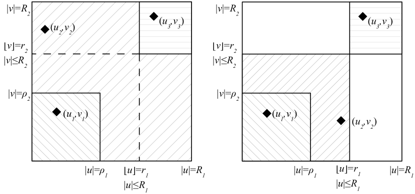
Figure 1. Localization of the three solutions $(u_{i},v_{i})$ from Theorem 2.8 (on the left) and Theorem 2.9 (on the right).

Theorem 2.9.

Suppose that all the assumptions of Theorem 2.8 are satisfied with the condition (2.15) replaced by (2.18). Then $N$ has at least three fixed points $(u_{i},v_{i})\in C$ $\left(i=1,2,3\right)$ with

$$|u_{1}| < \rho_{1},\ \ |v_{1}|<\rho_{2}\ \ (\text{possibly zero solution});$$

$$\left\lfloor u_{2}\right\rfloor < r_{1},\ \ \left\lfloor v_{2}\right\rfloor<r_{2};\ |u_{2}|>\rho_{1}\ \text{or }|v_{2}|>\rho_{2}\ \ (\text{possibly one solution component zero});$$

$$\left\lfloor u_{3}\right\rfloor > r_{1},\ \left\lfloor v_{3}\right\rfloor>r_{2}\ \ (\text{both solution components nonzero}).$$

Proof.

The assumption (2.18) implies both (2.4) and (2.10) and that there are no fixed points of $N$ on $\partial U$ and $\partial V.$ Hence, as in the proofs of Theorems 2.2 and 2.6, the indices $\mathrm{ind}_{C}(N,U)$ and $\mathrm{ind}_{C}(N,V)$ are well defined and equal $0.$ An analysis similar to that in the proof of Theorem 2.8 shows that

$$\mathrm{ind}_{C}(N,W)=1,\ \mathrm{ind}_{C}(N,U\setminus\overline{W})=-1,\ \mathrm{ind}_{C}(N,C\setminus\overline{V})=1,$$

which completes the proof. ∎

In order to ensure that the solution $(u_{1},v_{1})$ from the theorems above is nonzero, and thereby to obtain three nonzero solutions, we use some additional assumptions on $N$.

Theorem 2.10.

Assume that all the conditions of Theorem 2.8 or Theorem 2.9 are satisfied. Consider $0<\varrho_{i}<\left\lfloor\psi_{i}\right\rfloor\rho_{i},$ $i=1,2.$

(i) If $N_{1}(0,0)\neq 0$ or $N_{2}(0,0)\neq 0$, then the solution $(u_{1},v_{1})$ from Theorem 2.8 or 2.9 is nonzero.

(ii) If

(2.19) $$\inf\limits_{\begin{subarray}{c}(u,v)\in K,|u|\leq\rho_{1},|v|\leq\rho_{2}\\ \left\lfloor u\right\rfloor=\varrho_{1},\left\lfloor v\right\rfloor\geq\varrho_{2}\end{subarray}}\left\lfloor N_{1}(u,v)\right\rfloor\geq\varrho_{1},\ \ \inf\limits_{\begin{subarray}{c}(u,v)\in K,|u|\leq\rho_{1},|v|\leq\rho_{2}\\ \left\lfloor u\right\rfloor\geq\varrho_{1},\left\lfloor v\right\rfloor=\varrho_{2}\end{subarray}}\left\lfloor N_{2}(u,v)\right\rfloor\geq\varrho_{2}$$

and

$$|N_{i}(u,v)|\leq\rho_{i}\ \ \text{for\ \ }|u|\leq\rho_{1},\ |v|\leq\rho_{2}\ \ \ \left(i=1,2\right),$$

then we can assume that the solution $(u_{1},v_{1})$ from Theorem 2.8 or Theorem 2.9 satisfies $\left\lfloor u_{1}\right\rfloor\geq\varrho_{1}$ and $\left\lfloor v_{1}\right\rfloor\geq\varrho_{2}$;

(iii) if

(2.20) $$\inf\limits_{\begin{subarray}{c}(u,v)\in K,|u|\leq\tilde{\rho}_{1},|v|\leq\tilde{\rho}_{2}\\ \left\lfloor u\right\rfloor<\varrho_{1},\left\lfloor v\right\rfloor<\varrho_{2}\end{subarray}}\left\lfloor N_{1}(u,v)\right\rfloor\geq\varrho_{1}\ {\text{ or }}\ \inf\limits_{\begin{subarray}{c}(u,v)\in K,|u|\leq\tilde{\rho}_{1},|v|\leq\tilde{\rho}_{2}\\ \left\lfloor u\right\rfloor<\varrho_{1},\left\lfloor v\right\rfloor<\varrho_{2}\end{subarray}}\left\lfloor N_{2}(u,v)\right\rfloor\geq\varrho_{2}$$

for some$\ \tilde{\rho}_{1}\leq\rho_{1},\ \tilde{\rho}_{2}\leq\rho_{2},$ then we can assume that the solution $(u_{1},v_{1})$ from Theorem 2.8 or Theorem 2.9 satisfies $\left\lfloor u_{1}\right\rfloor\geq\varrho_{1}$ or $\left\lfloor v_{1}\right\rfloor\geq\varrho_{2}$ or $|u_{1}|>\tilde{\rho}_{1}$ or $|v_{1}|>\tilde{\rho}_{2}.$

Proof.

(i) The assumption impies that $(0,0)$ is not a fixed point.

(ii) The inequality follows from Theorem 2.6 applied in the case of $r_{i}:=\varrho_{i}$ and $R_{i}:=\rho_{i}.$

(iii) From Theorem 2.7 applied in the case of $r_{i}:=\varrho_{i},$ $R_{i}:=\rho_{i}$ and

$$A=\mbox{$\left\{(u,v):\;\left\lfloor u\right\rfloor<\varrho_{1},\left\lfloor v\right\rfloor<\varrho_{2},|u|\leq\tilde{\rho}_{1},|v|\leq\tilde{\rho}_{2}\right\}$},$$

we obtain there are no fixed points of $N$ in $A$, which ends the proof. ∎

The next Remark illustrates how Theorem 2.6 can be used to prove the existence of more nontrivial solutions.

Remark 2.11.

If $N$ satisfies the conditions of Theorem 2.6 for all pairs

$$0<r_{i}^{j}<\left\lfloor\psi_{i}\right\rfloor R_{i}^{j}\ \text{for }\ i=1,2,\ j=1,2,\ldots,n,$$

satisfying

$$\left\lfloor\psi_{i}\right\rfloor R_{i}^{j}<r_{i}^{j+1}\ \text{ for }\ i=1,2,\ j=1,2,\ldots,n-1,$$

then $N$ possesses at least $n$ nontrivial solutions $(u_{j},v_{j})$ with

$$|u_{j}|\leq R_{1}^{j},\ |v_{j}|\leq R_{2}^{j},\ \left\lfloor u_{j}\right\rfloor>r_{1}^{j},\ \left\lfloor v_{j}\right\rfloor>r_{2}^{j}.$$

Moreover, if (2.11) holds with the strict inequality, i.e. if

$$\sup\limits_{(u,v)\in K,|u|\leq R_{1}^{j},|v|\leq R_{2}^{j}}|N_{i}(u,v)|<R_{i}^{j}\quad(i=1,2),$$

hold, then we have $n-1$ additional solutions $(\bar{u}_{j},\bar{v}_{j}),$ $j=1,\ldots,n-1$ such that

$$|\bar{u}_{j}|<R_{1}^{j+1},\ |\bar{v}_{j}|<R_{2}^{j+1};\ |\bar{u}_{j}|>R_{1}^{j}\text{ or }|\bar{v}_{j}|>R_{2}^{j};\ \left\lfloor\bar{u}_{j}\right\rfloor<r_{1}^{j+1}\text{ or }\left\lfloor\bar{v}_{j}\right\rfloor<r_{2}^{j+1}.$$

The first conclusion follows from Theorem 2.6 applied $n$ times, whereas the second follows from Theorem 2.8 applied $n-1$ times.

Remark 2.12.

We stress that the abstract results obtained in this section can be applied to the case of one equation. Furthermore, our results can be generalized to the case of systems of more than two equations. The idea is to consider the product space $E=\Pi_{i=1}^{n}E_{i}$ of the Banach spaces $E_{i},$ endowed with the norms $|\cdot|_{i},$ functionals $\left\lfloor\cdot\right\rfloor_{i}$, and the pairs of cones and wedges $K_{i}\subset G_{i}\subset E_{i}$ such that (2.1), (2.2) are satisfied for $i=1,2,...,n.$ In this setting we are interested in the existence and localization of fixed points of a given operator $N\colon K\rightarrow K,$ where $K=\Pi_{i=1}^{n}K_{i}.$ For example, let us consider the sets

$$C=\mbox{$\left\{u\in K:\;|u_{1}|_{1}\leq R_{1},\ldots,|u_{n}|_{n}\leq R_{n}\right\}$},\ U=\mbox{$\left\{u\in C:\;\left\lfloor u_{1}\right\rfloor_{1}<r_{1},\ldots,\left\lfloor u_{n}\right\rfloor_{n}<r_{n}\right\}$}$$

for given radii $r_{i},R_{i}>0$ with $r_{i}<\left\lfloor\psi_{i}\right\rfloor_{i}R_{i},\$ $i=1,...,n.$ If

$$\sup_{u\in C}|N_{i}(u)|_{i}\leq R_{i},\ \ i=1,2,...,n$$

and

$$\inf_{\begin{subarray}{c}u\in\overline{U}\\ \left\lfloor u_{i}\right\rfloor_{i}=r_{i}\end{subarray}}\left\lfloor N_{i}(u)\right\rfloor_{i}>r_{i},\quad i=1,2,...,n,$$

then $N$ has at least one fixed point in $C\setminus\overline{U}.$

As a consequence, results analogous to ones obtained later in Section 3, can be established for systems with more than two differential equations.

3. The system of parabolic equations

Let $\Omega\subset\mathbb{R}^{m}$ be a bounded domain that is Dirichlet regular. This class of domains is rather large; for example, if the boundary of $\Omega$ is Lipschitz continuous, then $\Omega$ is Dirichlet regular (see [11, Chapter II, Section 4, Proposition 4]).

Let us take

$$E=C_{0}(\Omega)=\mbox{$\left\{u\in C(\overline{\Omega}):\;u|\partial\Omega=0\right\}$},\ E_{+}=\mbox{$\left\{u\in E:\;u(x)\geq 0\text{ for all }x\in\Omega\right\}$}.$$

Let us also consider the space ${\mathcal{E}}=C(0,{t_{\text{max}}},E)$, ${t_{\text{max}}}>0$ and its cone of nonnegative functions ${\mathcal{E}}_{+}=C(0,{t_{\text{max}}},E_{+})$. The spaces $E$ and ${\mathcal{E}}$ are endowed with the uniform norms, that is

$$|u|=\max\mbox{$\left\{|u(x)|:\;x\in\overline{\Omega}\right\}$},\ u\in E,$$

and

$$|u|=\max\mbox{$\left\{|u(t)|:\;0\leq t\leq{t_{\text{max}}}\right\}$},\ u\in{\mathcal{E}}.$$

Let $D\subset\subset\Omega$ be any open non-empty subset. Put

$${G}=\mbox{$\left\{u\in{\mathcal{E}}:\;u(0,x)\geq 0\ \text{ for all }x\in D\right\}$}.$$

The set $G$ is a wedge generating the semiorder $\preceq$. By $\leq$ we denote the order induced by the cone ${\mathcal{E}}_{+}$. The symbol $\leq$ will also be used to denote the order on $E$ induced by $E_{+}$ and the natural order on $H=L^{2}(\Omega)$ (that is $u\leq v$ if $u(x)\leq v(x)$ for a.a. $x\in\Omega$).

Given a function $u\in H$ we set

$$\left\lfloor u\right\rfloor=\operatorname*{ess\,inf}_{x\in D}|u(x)|,$$

(in particular $\left\lfloor u\right\rfloor=\inf_{x\in D}|u(x)|$ for $u\in E$) and futhermore, with abuse of notation, by the same symbol we denote the value $\left\lfloor u\right\rfloor=\left\lfloor u(0)\right\rfloor$ for $u\in{\mathcal{E}}$.

The following monotonicity and continuity conditions of the functional $\left\lfloor\cdot\right\rfloor$ are satisfied:

$$\left\lfloor u\right\rfloor\leq\left\lfloor v\right\rfloor\text{ if }u,v\in{\mathcal{E}}_{+}\text{ and }u\preceq v$$

and

$$|\left\lfloor u\right\rfloor-\left\lfloor v\right\rfloor|\leq|u-v|\text{ for all }u,v\in{\mathcal{E}}\quad\left(\text{therefore}\left\lfloor u\right\rfloor\leq|u|\text{ for all }u\in{\mathcal{E}}\right).$$

Consider the function $\psi(t)=\varphi$ for all $t\in[0,{t_{\text{max}}}]$, where $\varphi\in E$ satisfies the following conditions: $\varphi|D\equiv 1$ and $0\leq\varphi\leq 1$ in $\Omega$. Then $|\psi|=1$ and $u\preceq|u|\psi$ for every $u\in{\mathcal{E}}_{+}$.

Let us consider the Laplace operator $\Delta$ defined on the domain $D(\Delta)=\mbox{$\left\{u\in E:\;\Delta u\in E\right\}$}$. We briefly recall some known facts regarding the Laplace operator and the semigroup generated by it.

Lemma 3.1.

The operator $\Delta$ is a generator of an analytic (immediately) compact $C_{0}$-semigroup of contractions $\left\{S(t):\;t\geq 0\right\}$ on $E$. Moreover, the operators $S(t)$ are positive, i.e. $S(t)u\geq 0$ for $u\geq 0$.

Proof.

See [1, Section 6.1]. ∎

We shall also consider the space $H=L^{2}(\Omega)$ and the Laplacian $\Delta_{2}$ on $H$ with Dirichlet boundary condition. Denote by $S_{2}\colon[0,\infty)\to B(H)$ the semigroup generated by $\Delta_{2}$ and by $i\colon E\to H$ the natural embedding.

Proposition 3.2.

$i(S(t)u)=S_{2}(t)i(u)$ for all $u\in E$.

Proof.

The proof uses the Post-Widder inversion formula for $C_{0}$-semigroups (see Corollary 3.3.6 in [1]). ∎

Defnition 3.3.

For $\xi\in E$, and $f\in{\mathcal{E}}$, we say that the function

$$u(t)=p(\xi,f)(t):=S(t)\xi+\int_{0}^{t}S(t-s)f(s)ds$$

is a mild solution of the problem $u^{\prime}-\Delta u=f$ on $(0,{t_{\text{max}}})\times\Omega$ with $u(0)=\xi$.

It is worth pointing out the following regularity result of the mild solutions, this can be proved using standard techniques, see for example [31, Theorem 8.2.1].

Proposition 3.4.

Let $u=p(\xi,f)$ for $\xi\in E$, $f\in{\mathcal{E}}$, that is $u$ is a mild solution of the problem $u^{\prime}-\Delta u=f$, $u(0)=\xi$. Then

1. $u$ is a strong solution of that problem in the space $L^{2}(\Omega)$. Precisely, $u\colon[0,{t_{\text{max}}}]\to L^{2}(\Omega)$ is absolutely continuous, $u^{\prime}\in L^{1}(0,{t_{\text{max}}},L^{2}(\Omega))$, $u(t)\in D(\Delta_{2})$ and $u^{\prime}(t)=\Delta_{2}u(t)+f(t)$ for almost all $t\in(0,{t_{\text{max}}})$.

2. $u$ is a weak solution of the equation $u^{\prime}-\Delta_{2}u=f$ in the sense that the weak spatial derivative $\nabla u(t,x)$ and weak time derivative $u_{t}(t,x)$ exist on $(0,{t_{\text{max}}})\times\Omega$ and

   (3.1) $$\int_{0}^{t_{0}}\int_{\Omega}\nabla u(t,x)\nabla\phi(t,x)-u\frac{\partial}{\partial t}\phi(t,x)dxdt=\int_{0}^{t_{0}}\int_{\Omega}f(t)\phi(t,x)dt$$

   for all $\phi\in C^{\infty}_{0}((0,{t_{\text{max}}})\times\Omega)$.

We make use of the following result.

Proposition 3.5.

Assume that $u_{0}\in E$ is a nonnegative nonzero function. Define $u(t,x)=(S(t)u_{0})(x)$. Then

1. $u\in C^{\infty}((0,\infty)\times\Omega)\cap C(\mathbb{R}_{+}\times\overline{\Omega})$

2. $u_{t}=\Delta u$ on $(0,\infty)\times\Omega$

3. $u(0,x)=u_{0}(x)$ for $x\in\Omega$

4. $u(t,x)>0$ for $t>0$ and $x\in\Omega$.

Proof.

The conclusions (i)-(iii) follow from Proposition 2.6 of [1], while (iv) follows from the parabolic Harnack inequality, see for example Theorem 7.1.10 of [15]. ∎

Remark 3.6.

It seems worth discussing the choice of the space $C_{0}(\Omega)$. In the recent paper [19], where an elliptic system was discussed, the space $L^{\infty}(\Omega)$ was considered. Unfortunately, the Laplacian $\Delta$ fails to generate a $C_{0}$-semigroup on $L^{\infty}(\Omega)$. Moreover, although $\Delta$ generates semigroups on $L^{p}(\Omega)$, these spaces are somewhat inappropriate to obtain the localization of solutions with our approach. Note also that in the space ${\mathcal{E}}=C(0,{t_{\text{max}}},C_{0}(\Omega))$ there is no element $\bar{\psi}$ that $|\bar{\psi}|=1$ and $u\leq|u|\bar{\psi}$ for every $u\in{\mathcal{E}}_{+}$. This fact prevented us from using the abstract setting from [19] and is the main reason for considering the wedges $G_{i}$, $i\in\{1,2\}$, and the semiorders $\preceq$ in Section 2.

We make use of the following Lemma.

Lemma 3.7.

Let $0\neq\eta\in E=C_{0}(\Omega)$ and let $\mu$ be a Borel measure on $\mathbb{R}$.

1. If $0<t_{0}<t_{1}$, then we have

   $$m_{\eta}(t_{0},t_{1}):=\min\mbox{$\left\{(S(\tau)\eta)(x):\;x\in\overline{D},\ \tau\in[t_{0},t_{1}]\right\}$}>0.$$

2. If $0\leq t_{0}<t_{1}$ and $\mu([t_{0},t_{1}])>0$, then we have $\left\lfloor\int_{t_{0}}^{t_{1}}S(\tau)\eta d\mu(\tau)\right\rfloor>0$.

Proof.

(a) The conclusion follows from Proposition 3.5 and compactness of $[t_{0},t_{1}]\times\overline{D}$.

(b) We can assume that $t_{0}>0$. Then

$$\int_{t_{0}}^{t_{1}}(S(\tau)\eta)(x)d\mu(\tau)\geq\mu([t_{0},t_{1}])m_{\eta}(t_{0},t_{1})>0$$

for $x\in D$, which is the desired conclusion. ∎

Define

(3.2) $$m(t_{0},t_{1}):=\operatorname*{ess\,inf}_{x\in D,\ t\in[t_{0},t_{1}]}\left(S_{2}(t)\chi_{D}\right)(x).$$

Corollary 3.8.

1. If $0<t_{0}<t_{1}$, then $m(t_{0},t_{1})>0$.

2. If $0\leq t_{0}\leq t_{1}$ and $\mu([t_{0},t_{1}])>0$, then $\left\lfloor\int_{t_{0}}^{t_{1}}S_{2}(\tau)\chi_{D}d\mu(\tau)\right\rfloor>0$.

It is possible that $m(0,t_{1})>0$ (see Example 3.26).

Proof.

Let $\eta\in E=C_{0}(\Omega)$ be any nonzero function with $0\leq\eta\leq\chi_{D}$. The conclusion is implied by Lemma 3.7 and the inequality $S_{2}(t)\chi_{D}\geq S_{2}(t)\eta=S(t)\eta,$ which follows from the positiveness of $S_{2}$ and Proposition 3.2. ∎

Define the cones

$$K_{1}=K_{2}=\mbox{$\left\{u\in{\mathcal{E}}_{+}:\;u(t)\geq S(t)u(0)\ \text{for all}\ t\in[0,{t_{\text{max}}}]\right\}$}.$$

Let us fix $0\leq t_{0}<t_{1}\leq{t_{\text{max}}}$ satisfying $\mu_{1}([t_{0},t_{1}])>0$, $\mu_{1}([t_{0},t_{1}])>0$, where $\mu_{i}$ are the measures from the definition of $\alpha$ and $\beta$. Put $m:=m(t_{0},t_{1})$.

Remark 3.9.

Take $u\in K$ and set $r:=\left\lfloor u\right\rfloor=\inf_{x\in D}u(0,x)$. Observe that $u(0)\geq r\chi_{D}$ and therefore we have

$$u(t)\geq S(t)u(0)=S_{2}(t)u(0)\geq rS_{2}(t)\chi_{D}\geq rm\chi_{D}\ \text{ for }t\in[t_{0},t_{1}].$$

As a consequence, we obtain the estimate

(3.3) $$u\geq m\left\lfloor u\right\rfloor\chi_{[t_{0},t_{1}]\times D}\ \text{ for all }u\in K,$$

which can be called weak Harnack-type inequality, a counterpart of the inequality (3.4) of [19].

We now turn back our attention to the parabolic system

(3.4) $$\begin{cases}u_{t}-\Delta u=f(t,x,u,v)&(t,x)\in Q:=(0,{t_{\text{max}}})\times\Omega,\\ v_{t}-\Delta v=g(t,x,u,v)&(t,x)\in Q:=(0,{t_{\text{max}}})\times\Omega,\\ u(t,x)=v(t,x)=0&(t,x)\in(0,{t_{\text{max}}})\times\partial\Omega,\\ u(0,\cdot)=\alpha(u,v),\\ v(0,\cdot)=\beta(u,v).\end{cases}$$

Here, $f,g\colon(0,{t_{\text{max}}})\times\Omega\times\mathbb{R}_{+}\times\mathbb{R}_{+}\to\mathbb{R}_{+}$ and $\alpha,\beta\colon{\mathcal{E}}\times{\mathcal{E}}\to E$ are continuous functions. In what follows we shall identify $u\colon[0,{t_{\text{max}}}]\times\overline{\Omega}\to\mathbb{R}$ with $u\colon[0,{t_{\text{max}}}]\to C(\overline{\Omega})$ via the formula $u(t)(x)=u(t,x)$.

Define

$$F(u,v)(t)(x)=f(t,x,u(t)(x),v(t)(x)),\quad G(u,v)(t)(x)=g(t,x,u(t)(x),v(t)(x))).$$

Under the following assumption:

(3.5) $$f(t,x,0,0)=g(t,x,0,0)=0\ \text{ for }x\in\partial\Omega,$$

the operators $F,G\colon{\mathcal{E}}\times{\mathcal{E}}\to{\mathcal{E}}$ are continuous and bounded (map bounded sets into bounded ones).

Therefore, the mild solution of the problem (3.4) is a fixed point of the vector valued operator $M$ defined as

$$M_{1}(u,v)=\bar{S}(\alpha(u,v))+\hat{S}(F(u,v)),\ M_{2}(u,v)=\bar{S}(\beta(u,v))+\hat{S}(G(u,v)),$$

where

$$\bar{S}\colon E\to{\mathcal{E}},\ \bar{S}(u_{0})(t)=S(t)u_{0},\ u_{0}\in E,$$

$$\hat{S}\colon{\mathcal{E}}\to{\mathcal{E}},\ \hat{S}(f)(t)=\int_{0}^{t}S(t-\tau)f(\tau)d\tau,f\in{\mathcal{E}}.$$

Proposition 3.10.

The operators $M_{1},M_{2}$ are completely continuous if and only if $\alpha$ and $\beta$ are completely continuous.

Proof.

If $M_{1}$, $M_{2}$ are completely continuous, then $e_{0}\circ M_{1}=\alpha,e_{0}\circ M_{2}=\beta$ are completely continuous, where $e_{0}(f)=f(0)$ for $f\in{\mathcal{E}}$.

Now, assume that the operators $\alpha,\beta$ are completely continuous. Since the operator $\bar{S}$ is continuous, then the operator $\bar{S}\circ\alpha$ is completely continuous. We shall demonstrate that $\hat{S}$ is completely continuous. In order to do this we utilize a version of the Ascoli-Arzelà Theorem tailored for the space ${\mathcal{E}}$, see for example Theorem A.2.1 of [31].

First, denote by $\Xi$ the upper bound of the norms of $\|S(t)\|_{B(E)}$ for $t\in[0,{t_{\text{max}}}]$. Because $S$ is immediate norm continuous, for any $\varepsilon>0$ there exists a number $\delta(\varepsilon)>0$ such that $\|S(t)-S(s)\|_{B(E)}<\varepsilon$ if $0<\varepsilon\leq t\leq s\leq t+\delta(\varepsilon)$.

Fix $R,\varepsilon>0$ and let $D=\mbox{$\left\{f\in{\mathcal{E}}:\;|f|<R\right\}$}$. For a fixed $t>0$ and $f\in D$ let $\eta=\min\{t,\varepsilon\}$. We can present $\hat{S}(f)(t)$ as a sum $\hat{S}(t)=x+y$, where

$$x=S(\eta)\int_{0}^{t-\eta}S(t-s-\eta)f(s)ds,\quad y=\int_{t-\eta}^{t}S(t-s)f(s)ds.$$

It is straightforward to show that $x\in\hat{C}:=S(\eta)(B(0,t\Xi R))$ and that $y\in B(0,\varepsilon\Xi R)$. Because $\hat{C}$ is relatively compact and $\varepsilon$ is arbitrary, we obtain the set $\left\{\hat{S}(f)(t):\;f\in D\right\}$ is relatively compact for all $t\in[0,{t_{\text{max}}}]$.

Now we shall prove the equicontinuity of the family $\left\{\hat{S}(f):\;f\in D\right\}$. In order to do it let us fix $\varepsilon>0$, $t,s\in[0,{t_{\text{max}}}]$ and $f\in D$. Without loss of generality we can assume that $t\leq s$. Let us put $\eta=\min\{t,\varepsilon\}$ (the case $\eta=0$ appears if $t=0$). Then $\hat{S}(f)(s)-\hat{S}(f)(t)=x+y$, where

$$x=\int_{0}^{t}(S(s-\tau)f(\tau)-S(t-\tau)f(\tau))d\tau,\ y=\int_{t}^{s}S(s-\tau)f(\tau)d\tau.$$

$$|x|\leq R\int_{0}^{t}\|S(s-t+\tau)-S(\tau)\|_{B(E)}d\tau\leq 2\Xi R\varepsilon+\int_{\eta}^{t}\|S(s-t+\tau)-S(\tau)\|_{B(E)}d\tau.$$

$$|y|\leq|s-t|\Xi R.$$

Therefore $|\hat{S}(f)(s)-\hat{S}(f)(t)|\leq(3\Xi R+{t_{\text{max}}})\varepsilon$ if $|s-t|\leq\min\{\delta(\varepsilon),\varepsilon\}$. This proves the uniform equicontinuity of the family $\left\{\hat{S}(f):\;f\in D\right\}$ and finishes the proof of the complete continuity of $\hat{S}$. Now, the complete continuity of $M_{1}=\bar{S}\circ\alpha+\hat{S}\circ F$ is clear. Similarly we can prove the complete continuity of $M_{2}$. ∎

In order to use fixed point index for compact operators and, at the same time, to avoid assuming the compactness of $\alpha$ and $\beta$, we consider the operator $N=(N_{1},N_{2})$, defined by the formula

$$N_{1}(u,v)=\bar{S}\left(\alpha\left(\bar{S}(u(0))+\hat{S}(F(u,v))\>,\>\bar{S}(v(0))+\hat{S}(G(u,v))\right)\right)+\hat{S}(F(u,v)),$$

$$N_{2}(u,v)=\bar{S}\left(\beta\left(\bar{S}(u(0))+\hat{S}(F(u,v))\>,\>\bar{S}(v(0))+\hat{S}(G(u,v))\right)\right)+\hat{S}(G(u,v)).$$

Proposition 3.11.

The sets of fixed points of the operators $M$ and $N$ coincide.

Proof.

Note that

(3.6) $$N_{1}(u,v)=\bar{S}(u_{0})+\hat{S}(F(u,v))\text{ and }N_{2}(u,v)=\bar{S}(v_{0})+\hat{S}(G(u,v)),$$

where $u_{0}=\alpha(\bar{u},\bar{v})$, $v_{0}=\beta(\bar{u},\bar{v})$ and

(3.7) $$\bar{u}=\bar{S}(u(0))+\hat{S}(F(u,v)),\quad\bar{v}=\bar{S}(v(0))+\hat{S}(G(u,v)).$$

From (3.6) and the properties of $\bar{S}$ and $\hat{S}$ we have $N_{1}(u,v)(0)=u_{0}$ and $N_{2}(u,v)(0)=v_{0}$. Therefore, if $N(u,v)=(u,v)$, then $\bar{u}=u$ and $\bar{v}=v$ and, consequently, $u_{0}=\alpha(u,v)$ and $v_{0}=\beta(u,v)$. By (3.6) we arrive at $M(u,v)=(u,v)$.

Conversely, if $M(u,v)=(u,v)$, then

(3.8) $$u=\bar{S}(\alpha(u,v))+\hat{S}(F(u,v)),\ v=\bar{S}(\beta(u,v))+\hat{S}(G(u,v))$$

and $u(0)=\alpha(u,v)$, $v(0)=\beta(u,v)$. Therefore we have

$$u=\bar{S}(u(0))+\hat{S}(F(u,v))\text{ and }v=\bar{S}(v(0))+\hat{S}(F(u,v)).$$

Plugging this into (3.8) we obtain $N(u,v)=(u,v)$. ∎

From the proof it follows in particular, that

(3.9) $$\begin{array}[]{c}N_{1}(u,v)=\bar{S}(N_{1}(u,v)(0))+\hat{S}(F(u,v)),\text{ and }\\ N_{2}(u,v)=\bar{S}(N_{2}(u,v)(0))+\hat{S}(G(u,v)),\end{array}$$

which yields $N({\mathcal{E}}_{+}\times{\mathcal{E}}_{+})\subset K_{1}\times K_{2}=K$.

From Proposition 3.10 we know that a necessary condition for the operator $M$ to be completely continuous is the complete continuity of $\alpha$ and $\beta$. In the case of the operator $N$ we can weaken the assumptions on $\alpha$ and $\beta$.

Proposition 3.12.

The operator $N$ is completely continuous if the images $\alpha(U_{1}\times U_{2})$ and $\beta(U_{1}\times U_{2})$ are relatively compact for all bounded sets $U_{1},U_{2}\subset{\mathcal{E}}$ that satisfy the following property:

(3.10) $$\text{For all}\ \varepsilon>0\ \text{the set}\ \mbox{$\left\{u(t):\;u\in U_{i},\ t\in[\varepsilon,{t_{\text{max}}}]\right\}$}\ \text{is relatively compact},\ i=1,2.$$

Proof.

We prove, without loss of generality, the complete continuity of $N_{1}$. Let $\bar{\alpha}(u,v)=\alpha(\bar{u},\bar{v})$, where $\bar{u}(u,v)$ and $\bar{v}(u,v)$ are defined by (3.7). From (3.6) it follows that $N_{1}(u,v)=\bar{S}(\bar{\alpha}(u,v))+\hat{S}(F(u,v))$. By Proposition 3.10, it suffices to show that $\bar{\alpha}$ is completely continuous. This will be done if we demonstrate, that $\bar{u}(U\times U)$ and $\bar{v}(U\times U)$ satisfy (3.10) for a given bounded set $U\subset{\mathcal{E}}$.

Let $\varepsilon>0$ be given. Put $R=\sup\mbox{$\left\{|u|:\;u\in U\right\}$}$. For $u,v\in U$ and $t\geq\varepsilon$ we obtain

$$\bar{S}(u(0))(t)=S(\varepsilon)S(t-\varepsilon)u(0)\in S(\varepsilon)D(0,R)=:{\mathcal{C}}$$

and the set ${\mathcal{C}}$ is relatively compact. Moreover, the proof of Proposition 3.10 shows that the set $\hat{S}(F(U\times U))$ is relatively compact in $\mathcal{E}$. By the standard arguments, utilizing the compactness of $[0,{t_{\text{max}}}]$, one can show that the set

$$\left\{\hat{S}(F(u,v))(t):\;u,v\in U,\ t\in[0,{t_{\text{max}}}]\right\}$$

is totally bounded (and therefore relatively compact) in $E$. This shows that $\bar{u}(U\times U)$ satisfies the condition (3.10). Similarly we can verify this condition for the set $\bar{v}(U\times U)$. ∎

Example 3.13.

Let $\alpha(u,v)=u(t_{0})$, $\beta(u,v)=v(t_{0})$, where $0\leq t_{0}\leq{t_{\text{max}}}$. Then $\alpha,\beta$ satisfy the condition from Proposition 3.12 if and only if $t_{0}>0$. Indeed, let $t_{0}=0$ and $U_{1}=U_{2}=\mbox{$\left\{S(\cdot)u:\;|u|\leq 1\right\}$}$. Then the condition (3.10) is satisfied, but the set

$$\alpha(U_{1}\times U_{2})=\mbox{$\left\{u(0):\;u\in U_{1}\right\}$}=\mbox{$\left\{u\in E:\;|u|\leq 1\right\}$}$$

is not compact.

Conversely, if $t_{0}>0$ and sets $U_{1},U_{2}$ satisfy the condition (3.10), then $\alpha(U_{1}\times U_{2})=\mbox{$\left\{u(t_{0}):\;u\in U_{1}\right\}$}$ is compact from (3.10).

Proposition 3.14.

Let $\alpha,\beta$ be as in (1.2). Then $\alpha,\beta$ satisfy the assumptions of Proposition 3.12.

Proof.

Indeed, let us consider the sets $U_{1},U_{2}\subset B(0,R)$ satisfying the condition (3.10) and let $\varepsilon>0$. From the uniform continuity of $G_{1}$ on $[0,\omega\cdot d]$, where

$$d=\max\mbox{$\left\{g_{1}(u,v):\;0\leq u,v\leq R\right\}$},\ \omega=\mu_{1}([0,{t_{\text{max}}}]),$$

there exists $\delta>0$ such that $|G_{1}(p)-G_{1}(q)|<\varepsilon$ if $0\leq p,q\leq\omega\cdot d$, $|p-q|<\delta\cdot d$.

Since $\mu_{1}(\{0\})=0$, there exists $\sigma>0$ such that $\delta_{0}:=\mu_{1}([0,\sigma))<\delta$.

Put

$$U_{i}^{\sigma}:=\mbox{$\left\{u(t):\;u\in U_{i},\ t\in[\sigma,{t_{\text{max}}}]\right\}$},\ i=1,2\text{ and }\Gamma^{\sigma}:=\overline{\mathrm{conv}}\>g_{1}\!\left(U_{1}^{\sigma}\times U_{2}^{\sigma}\right).$$

From the Mazur Theorem, which states that the closed convex hull of a compact subset in a Banach space is compact, the set $\Gamma^{\sigma}$ is compact. Therefore,

$$\int_{\sigma}^{t_{\text{max}}}g_{1}(u(t),v(t))dt\in W^{\sigma}:=(\omega-\delta_{0})\cdot\Gamma^{\sigma}\ \text{ and }\ \left|\int_{0}^{\sigma}g_{1}(u(t),v(t))dt\right|\leq\delta\cdot d$$

for $u\in U_{1}$, $v\in U_{2}$. Thus, by the choice of $\delta$, we deduce that for all $u\in U_{1}$, $v\in U_{2}$ we have $\alpha(u,v)=u_{1}+u_{2}$, where $u_{1}\in G_{1}\!\left(W^{\sigma}\right)$ and $|u_{2}|<\varepsilon$. Because $G_{1}\!\left(W^{\sigma}\right)$ is compact and $\varepsilon$ is arbitrarily small, we obtain $\alpha(U_{1}\times U_{2})$ is relatively compact. Similarly we can proceed with $\beta$. ∎

Remark 3.15.

The assumption that $0$ is not an atom of the measures $\mu_{1},\mu_{2}$ follows from the observation from Example 3.13, where it is shown that the Dirac measure $\delta_{0}$ is not admissible in our theory. Moreover, in the case $\mu_{1}(\{0\})>0$ or $\mu_{2}(\{0\})>0$, the initial conditions $u(0)=\alpha(u,v)$, $v(0)=\beta(u,v)$ become implicit, making the considerations unnecessarily complicated or incorrect. Note also that the conclusion of Proposition 3.14 can be applied to the case of:

1. multi-point conditions of the type

   $$\alpha(u,v)=\sum_{s=1}^{k}\alpha_{s}u(t_{s}),\quad\beta(u,v)=\sum_{s=1}^{r}\beta_{s}v(t^{\prime}_{s}),$$

   where $0<t_{1}<\ldots<t_{k}$, $0<t^{\prime}_{1}<\ldots<t^{\prime}_{r}$ and $\alpha_{s},\beta_{s}>0$.

2. integral conditions of the type

   $$\alpha(u,v)=\int_{0}^{t_{\text{max}}}g_{1}(u(t))dt,\quad\beta(u,v)=\int_{0}^{t_{\text{max}}}g_{2}(v(t))dt.$$

Let $\alpha,\beta$ be as in (1.2). Consider the assumption

(3.11) $$p_{1}u\leq g_{1}(u,v)\leq q_{1}u,\ p_{2}v\leq g_{2}(u,v)\leq q_{2}v,\ P_{i}u\leq G_{i}(u)\leq Q_{i}u,$$

for all $u,v\geq 0$, $i\in\{1,2\}$, where $0<p_{i}\leq q_{i}$, $0<P_{i}\leq Q_{i}$, $i\in\{1,2\}$. Similar assumptions were used, for nonlinear nonlocal conditions in the context of ODEs, in [18, 20].

Under the assumption (3.11) we have the following estimates:

(3.12) $$\begin{split}p_{1}P_{1}\int_{0}^{{t_{\text{max}}}}u(t)d\mu_{1}(t)\leq\alpha(u,v)\leq q_{1}Q_{1}\int_{0}^{{t_{\text{max}}}}u(t)d\mu_{1}(t),\\ p_{2}P_{2}\int_{0}^{{t_{\text{max}}}}v(t)d\mu_{2}(t)\leq\beta(u,v)\leq q_{2}Q_{2}\int_{0}^{{t_{\text{max}}}}v(t)d\mu_{2}(t).\end{split}$$

Put

(3.13) $$f_{r,R}^{0}:=\inf\limits_{\begin{subarray}{c}t\in[t_{0},t_{1}],\ x\in D\\ mr_{1}\leq u\leq R_{1},\ 0\leq v\leq R_{2}\end{subarray}}\frac{f(t,x,u,v)}{r_{1}},\quad g_{r,R}^{0}:=\inf\limits_{\begin{subarray}{c}t\in[t_{0},t_{1}],\ x\in D\\ 0\leq u\leq R_{1},\ mr_{2}\leq v\leq R_{2}\end{subarray}}\frac{g(t,x,u,v)}{r_{2}},$$

(3.14) $$f_{r,R}:=\inf\limits_{\begin{subarray}{c}t\in[t_{0},t_{1}],\ x\in D\\ mr_{1}\leq u\leq R_{1},\ mr_{2}\leq v\leq R_{2}\end{subarray}}\frac{f(t,x,u,v)}{r_{1}},\quad g_{r,R}:=\inf\limits_{\begin{subarray}{c}t\in[t_{0},t_{1}],\ x\in D\\ mr_{1}\leq u\leq R_{1},\ mr_{2}\leq v\leq R_{2}\end{subarray}}\frac{g(t,x,u,v)}{r_{2}}$$

and

(3.15) $$f^{R}:=\sup\limits_{\begin{subarray}{c}t\in[0,{t_{\text{max}}}],\ x\in\Omega\\ 0\leq u\leq R_{1},\ 0\leq v\leq R_{2}\end{subarray}}\frac{f(t,x,u,v)}{R_{1}},\quad g^{R}:=\sup\limits_{\begin{subarray}{c}t\in[0,{t_{\text{max}}}],\ x\in\Omega\\ 0\leq u\leq R_{1},\ 0\leq v\leq R_{2}\end{subarray}}\frac{g(t,x,u,v)}{R_{2}}.$$

Note that we have $f_{r,R}^{0}\leq f_{r,R}\leq f^{R}$ and $g_{r,R}^{0}\leq g_{r,R}\leq g^{R}$.

Lemma 3.16.

Let $\alpha,\beta$ be as in (1.2).

Assume that the inequalities (3.11) are satisfied.

1. If $|u|\leq R_{1}$, $|v|\leq R_{2}$, then we have

   $$\frac{|N_{1}(u,v)|}{R_{1}}\leq q_{1}Q_{1}C_{1}^{1}+f^{R}(q_{1}Q_{1}C_{2}^{1}+C_{1}^{\prime}),\quad\frac{|N_{2}(u,v)|}{R_{2}}\leq q_{2}Q_{2}C_{1}^{2}+g^{R}(q_{2}Q_{2}C_{2}^{2}+C_{1}^{\prime}),$$

   where the constants

   $$C_{1}^{i}= \left|\int_{0}^{t_{\text{max}}}S_{2}(\tau)\chi_{\Omega}d\mu_{i}(\tau)\right|,\ C_{1}^{\prime}=\left|\int_{0}^{t_{\text{max}}}S_{2}(\tau)\chi_{\Omega}d\tau\right|,$$

   $$C_{2}^{i}= \left|\int_{0}^{t_{\text{max}}}\int_{0}^{t}S_{2}(\tau)\chi_{\Omega}d\tau d\mu_{i}(t)\right|$$

   are positive.

2. The following implications hold:

   $$\left\lfloor u\right\rfloor\geq r_{1}\implies\frac{\left\lfloor N_{1}(u,v)\right\rfloor}{r_{1}}\geq p_{1}P_{1}(c_{1}^{1}+f_{r,R}^{0}c_{2}^{1}),$$

   $$\left\lfloor v\right\rfloor\geq r_{2}\implies\frac{\left\lfloor N_{2}(u,v)\right\rfloor}{r_{2}}\geq p_{2}P_{2}(c_{1}^{2}+g_{r,R}^{0}c_{2}^{2}),$$

   where the constants

   (3.16) $$c_{1}^{i}=\left\lfloor\int_{0}^{t_{\text{max}}}S_{2}(\tau)\chi_{D}d\mu_{i}(\tau)\right\rfloor,\ c_{2}^{i}=\left\lfloor\int_{t_{0}}^{t_{\text{max}}}\int_{t_{0}}^{\min\{t,t_{1}\}}S_{2}(t-\tau)\chi_{D}d\tau d\mu_{i}(t)\right\rfloor$$

   are positive.

3. If $\left\lfloor u\right\rfloor\geq r_{1}$ and $\left\lfloor v\right\rfloor\geq r_{2}$, then we have

   $$\frac{\left\lfloor N_{1}(u,v)\right\rfloor}{r_{1}}\geq p_{1}P_{1}(c_{1}^{1}+f_{r,R}c_{2}^{1}),\quad\frac{\left\lfloor N_{2}(u,v)\right\rfloor}{r_{2}}\geq p_{2}P_{2}(c_{1}^{2}+g_{r,R}c_{2}^{2}),$$

Proof.

Consider $u,v$ such that $|u|\leq R_{1}$, $|v|\leq R_{2}$.

(a) Using the symbols $u_{0}$, $\bar{u}$, $\bar{v}$ introduced in the proof of Proposition 3.11 and having in mind the equality $u_{0}=\alpha(\bar{u},\bar{v})$ and the estimates (3.12) we obtain

(3.17) $$\frac{1}{q_{1}Q_{1}}u_{0}\leq\int_{0}^{t_{\text{max}}}\bar{u}(t)d\mu_{1}(t).$$

Exploiting the equation (3.7) we obtain

(3.18) $$\int_{0}^{t_{\text{max}}}\bar{u}(t)d\mu_{1}(t)=\int_{0}^{t_{\text{max}}}S(t)u(0)d\mu_{1}(t)+\int_{0}^{t_{\text{max}}}\int_{0}^{t}S(t-\tau)F(u,v)(\tau)d\tau d\mu_{1}(t).$$

From (3.17), (3.18), (3.15) and the fact that $u\leq R_{1}\chi_{\Omega}$ it can be concluded that

(3.19) $$\frac{1}{q_{1}Q_{1}}u_{0}\leq R_{1}\int_{0}^{t_{\text{max}}}S_{2}(t)\chi_{\Omega}d\mu_{1}(t)+R_{1}f^{R}\int_{0}^{t_{\text{max}}}\int_{0}^{t}S_{2}(\tau)\chi_{\Omega}d\tau d\mu_{1}(t).$$

From (3.6), we obtain

(3.20) $$N_{1}(u,v)(t)=S(t)u_{0}+\int_{0}^{t}S(t-\tau)F(u,v)(\tau)d\tau\leq S(t)u_{0}+R_{1}f^{R}\int_{0}^{t_{\text{max}}}S_{2}(\tau)\chi_{\Omega}d\tau.$$

Combining (3.19) and (3.20) an applying the contractiveness of $S(t)$ gives

$$\frac{|N_{1}(u,v)|}{R_{1}}\leq q_{1}Q_{1}C_{1}^{1}+f^{R}(q_{1}Q_{1}C_{2}^{1}+C_{1}^{\prime}).$$

Similarly, we can obtain the estimate of $|N_{2}(u,v)|$.

(b) Assume now that $\left\lfloor u\right\rfloor\geq r_{1}$. Then $u(0)\geq r_{1}\chi_{D}$. From (3.3) and (3.13) we obtain

$$u(t)\geq mr_{1}\chi_{D}\text{ and }F(u,v)(t)\geq r_{1}f_{r,R}^{0}\chi_{D}\text{ for }t\in[t_{0},t_{1}].$$

Using the symbols $\bar{u},\bar{v}$ introduced in the proof of Proposition 3.11 we obtain

$$\frac{1}{p_{1}P_{1}}N_{1}(u,v)(0) =\frac{1}{p_{1}P_{1}}\alpha(\bar{u},\bar{v})\geq\int_{0}^{t_{\text{max}}}\bar{u}(t)d\mu_{1}(t)$$

$$=\int_{0}^{t_{\text{max}}}S(t)u(0)d\mu_{1}(t)+\int_{0}^{t_{\text{max}}}\int_{0}^{t}S(t-\tau)F(u,v)(\tau)d\tau d\mu_{1}(t)\geq$$

$$\geq r_{1}\int_{0}^{t_{\text{max}}}S_{2}(t)\chi_{D}d\mu_{1}(t)+r_{1}f_{r,R}^{0}\int_{t_{0}}^{t_{\text{max}}}\int_{t_{0}}^{\min\{t,t_{1}\}}S_{2}(t-\tau)\chi_{D}d\tau d\mu_{1}(t).$$

Using the superadditivity of $\left\lfloor\cdot\right\rfloor$ we obtain

$$\frac{\left\lfloor N_{1}(u,v)\right\rfloor}{r_{1}}\geq p_{1}P_{1}(c_{1}^{1}+f_{r,R}^{0}c_{2}^{1}).$$

In the same manner we can obtain the estimate of $\left\lfloor N_{2}(u,v)\right\rfloor$.

(c) Using the fact, that $\left\lfloor v\right\rfloor\geq r_{2}$ implies $v(t)\geq mr_{2}\chi_{D}$ and following the calculations analogous to those above, we obtain the conclusion.

The positiveness of the constants $c_{1}^{i},c_{2}^{i},C_{1}^{i},C_{2}^{i},C_{1}^{\prime}$, $i=1,2$, follows from Corollary 3.8. ∎

Remark 3.17.

As it was pointed out in Remark 3.9, the Harnack-type inequality (3.3) is an analogue of the inequality (3.4) of [19]. These two inequalities play a crucial role in obtaining the estimates from below and are utilized for the calculation of the fixed point index on some suitable subsets of a cone.

The difference between these two Harnack-type inequalities deserves a comment, as our choice to use the inequality (3.3) led us to build the new theory presented in Section 2. The inequality (3.4) of [19] was directly derived from a Harnack-type inequality given by Trudinger [29]. The natural counterpart in our context would be the parabolic Harnack inequality by Trudinger [30, Theorem 1.2], which is valid for all weak supersolutions $u$ of the equation $u_{t}-\Delta u=0$ (that is, functions $u\geq 0$ such that $u_{t}-\Delta u\geq 0$). This inequality could be expressed in the following manner:

(3.21) $$u\geq c\|u\|\chi_{Q_{-}},$$

where $c>0$ is a constant and

$$\|u\|=\int_{Q_{+}}|u(t,x)|dtdx,\ Q_{+}=\left[t^{0},t^{1}\right]\times D,\ Q_{-}=\left[t_{0},t_{1}\right]\times D$$

for $0<t^{0}<t^{1}<t_{0}<t_{1}\leq{t_{\text{max}}}$. However, the use of this inequality is somewhat unnatural and it seems that it leads to additional complication of the argument and to worse results. For the sake of brevity, we provide here only a brief explanation.

1) The inequality (3.21) gives a lower bound on the values of $u$ on $Q_{-}$, which depend on the values of $u$ on $Q_{+}$. The proof of Lemma 3.16(b) shows that it is more convenient to utilize the dependence of values $u|Q_{-}$ on values of $u|\{0\}\times D$, due to the presence of the nonlocal boundary condition $u(0,x)=\alpha(u,v)(x)$.

2) The inequality (3.3) is actually a consequence of the inequality $u\geq m\left\lfloor u\right\rfloor\chi_{[t_{0},t_{1}]\times D}$ used for $u(t)=S_{2}(t)\chi_{D}$, which follows from the very definition of $m$. On the other hand, the inequality (3.21) is more general in the sense that the constant $c$ is so chosen that a supersolution $u$ of the equation $u_{t}-\Delta u=0$ satisfies the estimate $u(t,x)\geq c$ on $Q_{-}$ whenever $\|u\|\geq 1$. This universality, which in other context proves to be very important, is not exploited in our consideration, and unfortunately, it effects in a negative way the constants arising in the lower bounds of the nonlinearities (the counterparts of $c_{1}$ and $c_{2}$). And lastly, those constants are more difficult to be established. In other words, having in mind the nature of the calculations from Lemma 3.16, the use of minimum $\left\lfloor u\right\rfloor$ is more convenient, natural and effective than the use of the integral seminorm $\|u\|$.

3.1. Existence results

We are now prepared to establish some sufficient conditions for the existence of nonnegative nontrivial solutions of the problem (3.4). In what follows we shall assume that $\alpha,\beta$ are as in (1.2) and that the estimates (3.11) is satisfied.

Theorem 3.18.

Assume there exist radii $0<r_{i}<R_{i}$, $i\in\{1,2\}$ such that

(3.22) $$q_{1}Q_{1}C_{1}^{1}+f^{R}(q_{1}Q_{1}C_{2}^{1}+C_{1}^{\prime})\leq 1,\quad q_{2}Q_{2}C_{1}^{2}+g^{R}(q_{2}Q_{2}C_{2}^{2}+C_{1}^{\prime})\leq 1$$

and

(3.23) $$p_{1}P_{1}(c_{1}^{1}+f_{r,R}c_{2}^{1})>1,\quad p_{2}P_{2}(c_{1}^{2}+g_{r,R}c_{2}^{2})>1.$$

Then there exists at least one nonnegative solution $(u,v)$ of the problem (3.4) such that $|u|\leq R_{1},$ $|v|\leq R_{2}$ and $\left\lfloor u\right\rfloor>r_{1}$, $\left\lfloor v\right\rfloor>r_{2}$.

Proof.

Lemma 3.16 implies that the conditions (2.4) and (2.5) are satisfied. Moreover, $r_{i}<\left\lfloor\psi_{i}\right\rfloor R_{i}$, since $\left\lfloor\psi_{i}\right\rfloor=1$. The assertion follows from Theorem 2.6. ∎

Remark 3.19.

It is worth mentioning that the condition $\left\lfloor u\right\rfloor>r_{1}$ implies $|u|>r_{1}$, which follows from both the definitions of $|\cdot|$ and $\left\lfloor\cdot\right\rfloor$ and from Remark 2.4.

Theorem 3.20.

Let $0<r_{1}<R_{1}$, $0<r_{2}<R_{2}$ and let $\tilde{R}_{1}\leq R_{1}$, $\tilde{R}_{2}\leq R_{2}$. Define the quantities

$$f_{r,\tilde{R}}^{00}:=\inf\limits_{\begin{subarray}{c}t\in[t_{0},t_{1}],\ x\in D\\ 0\leq u\leq\tilde{R}_{1},\ 0\leq v\leq\tilde{R}_{2}\end{subarray}}\frac{f(t,x,u,v)}{r_{1}},\quad g_{r,\tilde{R}}^{00}:=\inf\limits_{\begin{subarray}{c}t\in[t_{0},t_{1}],\ x\in D\\ 0\leq u\leq\tilde{R}_{1},\ 0\leq v\leq\tilde{R}_{2}\end{subarray}}\frac{g(t,x,u,v)}{r_{2}}.$$

Assume that the condition (3.22) is satisfied and that

(3.24) $$f_{r,\tilde{R}}^{00}\geq\left(p_{1}P_{1}c_{2}^{1}\right)^{-1}\ \text{ or }\ g_{r,\tilde{R}}^{00}\geq\left(p_{2}P_{2}c_{2}^{2}\right)^{-1}.$$

Then there exists a nontrivial nonnegative solution $(u,v)$ of (3.4) such that $|u|\leq R_{1}$, $|v|\leq R_{2}$ and

(3.25) $$\left\lfloor u\right\rfloor\geq r_{1}\text{ or }\left\lfloor v\right\rfloor\geq r_{2}\text{ or }|u|>\tilde{R}_{1}\text{ or }|v|>\tilde{R}_{2}.$$

In particular, if $\tilde{R}_{1}=R_{1}$ and $\tilde{R}_{2}=R_{2},$ then there exists a nontrivial nonnegative solution $(u,v)$ with either $\left\lfloor u\right\rfloor\geq r_{1}$ or $\left\lfloor v\right\rfloor\geq r_{2}$.

Proof.

As in the previous proof we know that the condition (2.12) from Theorem 2.7 is satisfied. Let

$$(u,v)\in A:=\mbox{$\left\{(u,v):\;\left\lfloor u\right\rfloor<r_{1},\ \left\lfloor v\right\rfloor<r_{2},\ |u|\leq\tilde{R}_{1},\ |v|\leq\tilde{R}_{2}\right\}$}.$$

In the same way as in the proof of Lemma 3.16(b) we can prove that

(3.26) $$\frac{\left\lfloor N_{1}(u,v)\right\rfloor}{r_{1}}\geq p_{1}P_{1}c_{2}^{1}f_{r,\tilde{R}}^{00},\ \frac{\left\lfloor N_{2}(u,v)\right\rfloor}{r_{2}}\geq p_{2}P_{2}c_{2}^{2}g_{r,\tilde{R}}^{00}\ \text{ for }|u|\leq\tilde{R}_{1}\text{ and }|v|\leq\tilde{R}_{2}.$$

Therefore, the assumption (3.24) implies the condition (2.13) is satisfied and we can apply Theorem 2.7 to obtain a solution $(u,v)\not\in A$. Clearly, this is equivalent to (3.25). ∎

Remark 3.21.

The importance of Theorem 3.20 consists in the fact that the assumption (3.24) involves only one component of the system nonlinearity $(f,g).$ Therefore, it allows different kind of growth of $f$ and $g$ near the origin. A similar remark also applies to the following theorem.

Theorem 3.22.

Assume there exist radii $0<\rho_{i}<r_{i}<R_{i}$, $i\in\{1,2\}$, such that

$$q_{1}Q_{1}C_{1}^{1}+f^{R}(q_{1}Q_{1}C_{2}^{1}+C_{1}^{\prime})\leq 1,\quad q_{2}Q_{2}C_{1}^{2}+g^{R}(q_{2}Q_{2}C_{2}^{2}+C_{1}^{\prime})\leq 1,$$

$$q_{1}Q_{1}C_{1}^{1}+f^{\rho}(q_{1}Q_{1}C_{2}^{1}+C_{1}^{\prime})\leq 1,\quad q_{2}Q_{2}C_{1}^{2}+g^{\rho}(q_{2}Q_{2}C_{2}^{2}+C_{1}^{\prime})\leq 1$$

and

(3.27) $$p_{1}P_{1}(c_{1}^{1}+f_{r,R}c_{2}^{1})>1,\quad p_{2}P_{2}(c_{1}^{2}+g_{r,R}c_{2}^{2})>1$$

Then there exist three nonnegative solutions $(u_{i},v_{i})$ ($i=1,2,3$) of the system (3.4) with

$$|u_{1}| <\rho_{1},\ |v_{1}|<\rho_{2}\ (\text{possibly the zero solution});$$

$$\left\lfloor u_{2}\right\rfloor <r_{1}\text{ or }\left\lfloor v_{2}\right\rfloor<r_{2};\ |u_{2}|>\rho_{1}\text{ or }|v_{2}|>\rho_{2}\ (\text{possibly one solution component zero});$$

$$\left\lfloor u_{3}\right\rfloor >r_{1},\ \left\lfloor v_{3}\right\rfloor>r_{2}\ (\text{both solution components nonzero}).$$

By the following slight strengthening of the assumption (3.27):

(3.28) $$p_{1}P_{1}(c_{1}^{1}+f_{r,R}^{0}c_{2}^{1})>1,\quad p_{2}P_{2}(c_{1}^{2}+g_{r,R}^{0}c_{2}^{2})>1$$

we obtain a slight improvement of the precision in localizing the second solution:

$$\left\lfloor u_{2}\right\rfloor<r_{1},\ \left\lfloor v_{2}\right\rfloor<r_{2};\ |u_{2}|>\rho_{1}\ \text{or }|v_{2}|>\rho_{2}.$$

Moreover, having given numbers $0<\varrho_{i}<\rho_{i}$ ($i=1,2$),

(i) if

$$p_{1}P_{1}(c_{1}^{1}+f_{\varrho,\rho}c_{2}^{1})>1,\quad p_{2}P_{2}(c_{1}^{2}+g_{\varrho,\rho}c_{2}^{2})>1,$$

then $\left\lfloor u_{1}\right\rfloor\geq\varrho_{1}$ and $\left\lfloor v_{1}\right\rfloor\geq\varrho_{2}$;

(ii) if

$$f_{\varrho,\tilde{\rho}}^{00}\geq\left(p_{1}P_{1}c_{2}^{1}\right)^{-1}\ \text{ or }\ g_{\varrho,\tilde{\rho}}^{00}\geq\left(p_{2}P_{2}c_{2}^{2}\right)^{-1}$$

for some $\tilde{\rho}_{1}\leq\rho_{1},$ $\tilde{\rho}_{2}\leq\rho_{2}$, then $\left\lfloor u_{1}\right\rfloor\geq\varrho_{1}$ or $\left\lfloor v_{1}\right\rfloor\geq\varrho_{2}$ or $|u_{1}|>\tilde{\rho}_{1}$ or $|v_{1}|>\tilde{\rho}_{2}$.

Proof.

One can use Lemma 3.16. The first assertion follows from Theorem 2.8, while second follows from Theorem 2.9. The third part of the conclusion, i.e. assertions (i) and (ii), is a consequence of Theorem 2.10 and (3.26). ∎

3.2. Non-existence results

We now present some sufficient conditions for the non-existence of positive solutions of the system (3.4). We still assume that $\alpha,\beta$ are as in Example 3.14 and that (3.11) is satisfied. We also assume that ${t_{\text{max}}}\in\mathrm{supp}(\mu_{i})$, $i=1,2$.

Lemma 3.23.

Let $(u,v)$ be a solution of the system (3.4). If $u\neq 0$ then $\left\lfloor u\right\rfloor>0$ and if $v\neq 0$ then $\left\lfloor v\right\rfloor>0$.

Proof.

Let $0\leq t_{0}<{t_{\text{max}}}$ be such that $u(t_{0})\neq 0$. From Proposition 3.11 we know that $(u,v)$ is a fixed point of $M$. Thus,

$$\left\lfloor u(0)\right\rfloor=\left\lfloor\alpha(u,v)\right\rfloor\geq p_{1}P_{1}\left\lfloor\int_{0}^{t_{\text{max}}}u(t)d\mu_{1}(t)\right\rfloor\geq p_{1}P_{1}\left\lfloor\int_{t_{0}}^{t_{\text{max}}}u(t)d\mu_{1}(t)\right\rfloor$$

and $u(t)\geq S(t-t_{0})u(t_{0})$ for $t\geq t_{0}$. From Lemma 3.7 we therefore obtain

$$\left\lfloor u\right\rfloor=\left\lfloor u(0)\right\rfloor\geq p_{1}P_{1}\left\lfloor\int_{0}^{{t_{\text{max}}}-t_{0}}S(t)u(t_{0})d\mu_{1}(t+t_{0})\right\rfloor>0.$$

∎

Theorem 3.24.

Put

$$\overline{e}_{i}=\max\left(\frac{1-q_{i}Q_{i}C_{1}^{i}}{q_{i}Q_{i}C_{2}^{i}+C_{1}^{\prime}},\frac{1-q_{i}Q_{i}\mu_{i}([0,{t_{\text{max}}}])}{C_{1}^{\prime}}\right),\quad\underline{e}_{i}=\frac{(p_{i}P_{i})^{-1}-c_{1}^{i}}{mc_{2}^{i}},\ i\in\{0,1\}.$$

Assume that $(u_{0},v_{0})$ is a nonnegative solution of the system (3.4). If one of the following conditions holds:

(3.29) $$f(t,x,u,v)<\overline{e}_{1}u \text{ for all }t\in[0,{t_{\text{max}}}],\ x\in\Omega,\ u>0,\ v\geq 0,$$

(3.30) $$f(t,x,u,v)>\underline{e}_{1}u \text{ for all }t\in[t_{0},t_{1}],\ x\in D,\ u>0,\ v\geq 0,$$

then $u_{0}=0$.

Similarly, if one of the following conditions holds:

(3.31) $$g(t,x,u,v)<\overline{e}_{2}v \text{ for all }t\in[0,{t_{\text{max}}}],\ x\in\Omega,\ u\geq 0,\ v>0,$$

(3.32) $$g(t,x,u,v)>\underline{e}_{2}v \text{ for all }t\in[t_{0},t_{1}],\ x\in D,\ u\geq 0,\ v>0,$$

then $v_{0}=0$.

In particular, if $p_{1}P_{1}c_{1}^{1}>1$ ($p_{2}P_{2}c_{1}^{2}>1$), then $u_{0}=0$ ($v_{0}=0$), regardless of the properties of $f$ ($g$).

Proof.

Suppose on the contrary that $u_{0}\neq 0$. Then $u_{0}=N_{1}(u_{0},v_{0})=M_{1}(u_{0},v_{0})$. Put $R_{1}=|u_{0}|$, $R_{2}=\max\{|v_{0}|,1\}$ and $r_{1}=\left\lfloor u_{0}\right\rfloor>0$.

Assume that the inequality (3.29) holds. Observe that $f(t,x,u,v)/R_{1}<\overline{e}_{1}$ for $t\in[0,{t_{\text{max}}}]$, $x\in\overline{\Omega}$, $0\leq u\leq R_{1}$ and $0\leq v\leq R_{2}$. Therefore, $f^{R}<\overline{e}_{1}$. From Lemma 3.16(a) we obtain

(3.33) $$1=\frac{|u_{0}|}{R_{1}}=\frac{|N_{1}(u_{0},v_{0})|}{R_{1}}\leq q_{1}Q_{1}C_{1}^{1}+f^{R}(q_{1}Q_{1}C_{2}^{1}+C_{1}^{\prime}).$$

Similarly, in the analogous manner as in the proof of Lemma 3.16(a), one can show that

(3.34) $$1=\frac{|u_{0}|}{R_{1}}=\frac{|M_{1}(u_{0},v_{0})|}{R_{1}}\leq q_{1}Q_{1}\mu_{1}([0,{t_{\text{max}}}])+f^{R}C_{1}^{\prime}.$$

The estimates (3.33) and (3.34) give $f^{R}\geq\overline{e}_{1}$, a contradiction.

Assume now that (3.30) holds. Observe that $f(t,x,u,v)/r_{1}>m\underline{e}_{1}$ for $t\in[t_{0},t_{1}]$, $x\in D$, $mr_{1}\leq u\leq R_{1}$ and $0\leq v\leq R_{2}$. Therefore, $f_{r,R}^{0}>m\underline{e}_{1}$.

On the other hand, from Lemma 3.16(b) we obtain

(3.35) $$1=\frac{\left\lfloor u_{0}\right\rfloor}{r_{1}}=\frac{\left\lfloor N_{1}(u_{0},v_{0})\right\rfloor}{r_{1}}\geq p_{1}P_{1}(c_{1}^{1}+f_{r,R}^{0}c_{2}^{1}).$$

From (3.35) we conclude that $f_{r,R}^{0}\leq m\underline{e}_{1}$, a contradiction.

The second assertion can be proved analogously. ∎

Corollary 3.25.

(i) If one of the inequalities (3.29)-(3.32) holds, then there are no positive solutions of the system (3.4).

(ii) If one of the inequalities (3.29)-(3.30) holds and one of the inequalities (3.31)-(3.32) holds, then there are no nontrivial nonnegative solutions of the system (3.4).

3.3. Two examples

In the following one-dimensional examples we show that all the constants $C_{1}^{i}$, $C_{1}^{\prime}$, $C_{2}^{i}$, $c_{1}^{i}$, $c_{2}^{i}$, $m$, $i=1,2$, that occur in our theory can be computed.

Example 3.26.

Let $\Omega=[0,\pi]$ and let $\mu_{1}=\mu_{2}$ be the Lebesgue measure on $[0,{t_{\text{max}}}]$. Let us put $D=[b,\pi-b]$ for a fixed $0<b<\pi/2$. Then

$$\chi_{D}=\sum_{k=0}^{\infty}\frac{4}{(2k+1)\pi}\cos\big{(}(2k+1)b\big{)}\cdot\sin\big{(}(2k+1)x\big{)}$$

and

$$\chi_{\Omega}=\sum_{k=0}^{\infty}\frac{4}{(2k+1)\pi}\sin\big{(}(2k+1)x\big{)},$$

where the convergence is considered in the space $L^{2}(\Omega)$.

The evolution of $\chi_{D}$ and $\chi_{\Omega}$ is given by the formulae

$$(S_{2}(t)\chi_{D})(x)=\sum_{k=0}^{\infty}\frac{4}{(2k+1)\pi}\cos\big{(}(2k+1)b\big{)}\cdot e^{-(2k+1)^{2}t}\cdot\sin\big{(}(2k+1)x\big{)},$$

$$(S_{2}(t)\chi_{\Omega})(x)=\sum_{k=0}^{\infty}\frac{4}{(2k+1)\pi}\cdot e^{-(2k+1)^{2}t}\cdot\sin\big{(}(2k+1)x\big{)}.$$

Put $b=\pi/4$, $t_{0}=0$ and $t_{1}={t_{\text{max}}}=1$. Then we have

$$m=(S_{2}(1)\chi_{D})\left(\frac{\pi}{4}\right)=\sum_{k=0}^{\infty}(-1)^{k}\frac{2}{(2k+1)\pi}e^{-(2k+1)^{2}}\approx 0.23.$$

Since we consider the Lebesgue measure in the definition of the operators $\alpha$ and $\beta$, we shall omit the superscripts in the constants $C_{j}^{i}$, $c_{j}^{i}$.

Because

$$\int_{0}^{t_{\text{max}}}S_{2}(\tau)\chi_{D}d\tau(x)=\sum_{k=0}^{\infty}\frac{4}{(2k+1)^{3}\pi}\cos(2k+1)\frac{\pi}{4}\cdot\left(1-e^{-(2k+1)^{2}}\right)\cdot\sin\big{(}(2k+1)x\big{)}$$

and

$$\int_{0}^{t_{\text{max}}}\int_{0}^{t}S_{2}(t-\tau)\chi_{D}d\tau dt=\sum_{k=0}^{\infty}\frac{4}{(2k+1)^{5}\pi}\cos(2k+1)\frac{\pi}{4}\cdot e^{-(2k+1)^{2}}\cdot\sin\big{(}(2k+1)x\big{)},$$

we obtain

$$c_{1}=\sum_{k=0}^{\infty}\frac{2\cdot(-1)^{k}}{(2k+1)^{3}\pi}\left(1-e^{-(2k+1)^{2}}\right)\approx 0.38$$

and

$$c_{2}=\sum_{k=0}^{\infty}\frac{2\cdot(-1)^{k}}{(2k+1)^{5}\pi}e^{-(2k+1)^{2}}\approx 0.23$$

Moreover, because

$$\int_{0}^{t_{\text{max}}}S_{2}(\tau)\chi_{\Omega}d\tau=\sum_{k=0}^{\infty}\frac{4}{(2k+1)^{3}\pi}\cdot\left(1-e^{-(2k+1)^{2}}\right)\cdot\sin\big{(}(2k+1)x\big{)}$$

and

$$\int_{0}^{t_{\text{max}}}\int_{0}^{t}S_{2}(\tau)\chi_{\Omega}d\tau dt=\sum_{k=0}^{\infty}\frac{4}{(2k+1)^{5}\pi}\cdot e^{-(2k+1)^{2}}\cdot\sin\big{(}(2k+1)x\big{)},$$

(3.36) $$C_{1}=\left|\int_{0}^{t_{\text{max}}}S_{2}(\tau)\chi_{\Omega}d\tau\right|,\quad C_{2}=\left|\int_{0}^{t_{\text{max}}}\int_{0}^{t}S_{2}(\tau)\chi_{\Omega}d\tau dt\right|$$

we obtain

$$C_{1}=C_{1}^{\prime}=\sum_{k=0}^{\infty}\frac{4\cdot(-1)^{k}}{(2k+1)^{3}\pi}\cdot\left(1-e^{-(2k+1)^{2}}\right)\approx 0.77$$

and

$$C_{2}=\sum_{k=0}^{\infty}\frac{4\cdot(-1)^{k}}{(2k+1)^{5}\pi}\cdot e^{-(2k+1)^{2}}\approx 0.47.$$

If we put $G_{i}(x)=g_{i}(x)=x$, then $p_{i}=P_{i}=q_{i}=Q_{i}=1$ and the conditions (3.22) and (3.23) are equivalent to the following inequalities:

$$f^{R},g^{R}\leq\frac{1-C_{1}}{C_{1}^{\prime}+C_{2}}\approx 0.19,\quad f_{r,R},g_{r,R}>\frac{1-c_{1}}{c_{2}}\approx 2.64.$$

The numerical calculations indicate that the choice $b=\pi/4$ is optimal, i.e. the ratio $(1-c_{1})/(c_{2}m)$ is the smallest.

Example 3.27.

Let $\Omega,D,{t_{\text{max}}}$ be as in Example 3.26. We consider the problem (1.1) with conditions of the form $u(0)=\kappa u({t_{\text{max}}})$, $v(0)=\kappa v({t_{\text{max}}})$, $\kappa>0$. We discuss in details the cases of periodic conditions and of solutions that double in time. Therefore $u(0)=\alpha(u,v)$ and $v(0)=\beta(u,v)$, where $\alpha$ and $\beta$ are as in (1.2) with $G_{i}=\mathrm{id}$, $g_{i}(u_{1},u_{2})=\kappa\cdot u_{i}$ and $\mu_{1}=\mu_{2}=\delta_{{t_{\text{max}}}}$ is a Dirac measure. Hence we have $p_{i}=q_{i}=\kappa$ and $P_{i}=Q_{i}=1$. Put $t_{0}=0$ and $t_{1}={t_{\text{max}}}=1$.

The evolution of $\chi_{D}$ and $\chi_{\Omega}$ is the same as in Example 3.26. Therefore, $m\approx 0.23$. The remaining constants can be calculated by using the formulae

$$C_{1}=\left|S_{2}({t_{\text{max}}})\chi_{\Omega}\right|,\ C_{2}=C_{1}^{\prime}=\left|\int_{0}^{t_{\text{max}}}S_{2}(\tau)\chi_{\Omega}d\tau\right|,$$

$$c_{1}=\left\lfloor S_{2}({t_{\text{max}}})\chi_{D}\right\rfloor,\ c_{2}=\left\lfloor\int_{0}^{t_{\text{max}}}S_{2}(\tau)\chi_{D}d\tau\right\rfloor$$

and the calculations from Example 3.26. We obtain

$$C_{1}=\sum_{k=0}^{\infty}(-1)^{k}\frac{4}{(2k+1)\pi}e^{-(2k+1)^{2}}=2m\approx 0.46,\ C_{2}\approx 0.77,\ c_{1}=m\approx 0.23,\ c_{2}\approx 0.38.$$

Finally, the conditions (3.22) and (3.23) are equivalent to the following inequalities:

$$f^{R},g^{R}\leq\mathbf{C}(\kappa):=\frac{1-\kappa C_{1}}{C_{1}^{\prime}+\kappa C_{2}},\quad f_{r,R},g_{r,R}>\mathbf{c}(\kappa):=\frac{1-\kappa c_{1}}{\kappa c_{2}}.$$

For instance, in the periodic case ($\kappa=1$) we obtain $\mathbf{C}(1)\approx 0.35$ and $\mathbf{c}(1)\approx 2.03$. Moreover, in the case of solutions that double in time ($\kappa=0.5$) we obtain $\mathbf{C}(0.5)\approx 0.67$ and $\mathbf{c}(0.5)\approx 4.66$.

References

[1] W. Arendt, C. Batty, M. Hieber and F. Neubrander, Vector-valued Laplace transforms and Cauchy problems. Monographs in Mathematics, 96. Birkhäuser Verlag, Basel, 2001.
[2]
I. Benedetti, V. Taddei and M. Väth, Evolution problems with nonlinear nonlocal boundary conditions,
J. Dynam. Differential Equations25 (2013), 477–503.
[3] L. Byszewski, Strong maximum and minimum principles for parabolic problems with nonlocal inequalities, Z. Angew. Math. Mech., 70 (1990), 202–206.
[4] L. Byszewski, Strong maximum principles for parabolic nonlinear problems with nonlocal inequalities together with integrals, J. Appl. Math. Stochastic Anal., 3 (1990), 65–79.
[5] L. Byszewski, Strong maximum principles for parabolic nonlinear problems with nonlocal inequalities together with arbitrary functionals, J. Math. Anal. Appl., 156 (1991), 457–470.
[6] A. Boucherif,
Nonlocal problems for parabolic inclusions, Discrete Contin. Dyn. Syst., suppl. (2009), 82–91.
[7] A. Boucherif,
Discontinuous parabolic problems with a nonlocal initial condition, Bound. Value Probl., 2011, Art. ID 965759, 10 pp.
[8] A. Boucherif,
Nonlocal conditions for lower semicontinuous parabolic inclusions, Adv. Difference Equ., 2011, Art. ID 109570, 7 pp.
[9] T. Cardinali, R. Precup and P. Rubbioni, A unified existence theory for evolution equations and systems under nonlocal conditions, J. Math. Anal. Appl., 432 (2015), 1039–1057.
[10]
J. Chabrowski, On nonlocal problems for parabolic equations, Nagoya Math. J., 93 (1984), 109–131.
[11] R. Dautray and J. L. Lions, Mathematical analysis and numerical methods
for science and technology, Vol. 1–3. Springer-Verlag, Berlin, 1990.
[12] K. Deimling,
Nonlinear functional analysis,
Springer-Verlag, Berlin, 1985.
[13]
K. Deng, Exponential decay of solutions of semilinear parabolic equations with nonlocal initial conditions, J. Math. Anal. Appl., 179 (1993) 630–637.
[14] K. J. Engel and R. Nagel, One-parameter semigroups for linear evolution equations. Graduate Texts in Mathematics, 194. Springer-Verlag, New York, 2000.
[15] L. C. Evans, Partial differential equations. Graduate Studies in Mathematics, 19. American Mathematical Society, Providence, RI, 1998.
[16] A. Granas and J. Dugundji,
Fixed point theory,
Springer-Verlag, New York, 2003.
[17] D. Guo and V. Lakshmikantham,
Nonlinear problems in abstract cones, Academic Press, Boston, 1988.
[18] G. Infante,
Nonlocal boundary value problems with two nonlinear boundary conditions,
Commun. Appl. Anal., 12 (2008), 279-288.
[19] G. Infante, M. Maciejewski and R. Precup, A topological approach to the existence and multiplicity of positive solutions of -Laplacian systems, Dyn. Partial Differ. Equ., 12 (2015), 193-215.
[20] G. Infante and P. Pietramala,
Existence and multiplicity of non-negative solutions for systems of perturbed Hammerstein
integral equations, Nonlinear Anal., 71 (2009), 1301–1310.
[21] R. W. Leggett and L. R. Williams, Multiple positive fixed points of nonlinear operators on ordered Banach spaces, Indiana Univ. Math. J., 28 (1979), 673–688.
[22] M. A. McKibben, Discovering evolution equations with applications, vol. I. Chapman & Hall Mathematics, Boca Raton, 2011.
[23]
W. E. Olmstead and C. A. Roberts, The one-dimensional heat equation with a nonlocal initial condition, Appl. Math. Lett., 10 (1997), 89–94.
[24] C. V. Pao, Reaction diffusion equations with nonlocal boundary and nonlocal initial conditions, J. Math. Anal. Appl., 195 (1995), 702–718.
[25] R. Precup, Parabolic Harnack type inequalities and multiple positive solutions of evolution equations (preprint).
[26]
J. M. Rassias and E. T. Karimov, Boundary-value problems with non-local initial condition for parabolic equations with parameter, European J. Pure Appl. Math., 3 (2010) 948–957.
[27]
J. M. Rassias and E. T. Karimov, Boundary-value problems with non-local condition for degenerate parabolic equations, Contemporary Analysis and Applied Mathematics, Vol.1, No.1, 42-48, 2013.
[28] A. Štikonas, A survey on stationary problems, Green’s functions and spectrum of Sturm-Liouville problem
with nonlocal boundary conditions,
Nonlinear Anal. Model. Control, 19 (2014), 301–334.
[29] N. S. Trudinger, On Harnack type inequalities and their applications to quasilinear elliptic equations, Comm. Pure Appl. Math., 20 (1967), 721–747.
[30] N. S. Trudinger, Pointwise estimates and quasilinear parabolic equations, Comm. Pure Appl. Math.21 (1968), 205-226.
[31] I. I. Vrabie, -semigroups and applications. North-Holland Mathematics Studies, 191. North-Holland Publishing Co., Amsterdam, 2003.