Parallel Worldline Numerics: Implementation and Error Analysis

Abstract

We give an overview of the worldline numerics technique, and discuss the parallel CUDA implementation of a worldline numerics algorithm. In the worldline numerics technique, we wish to generate an ensemble of representative closed-loop particle trajectories, and use these to compute an approximate average value for Wilson loops. We show how this can be done with a specific emphasis on cylindrically symmetric magnetic fields. The fine-grained, massive parallelism provided by the GPU architecture results in considerable speedup in computing Wilson loop averages. Furthermore, we give a brief overview of uncertainty analysis in the worldline numerics method. There are uncertainties from discretizing each loop, and from using a statistical ensemble of representative loops. The former can be minimized so that the latter dominates. However, determining the statistical uncertainties is complicated by two subtleties. Firstly, the distributions generated by the worldline ensembles are highly non-Gaussian, and so the standard error in the mean is not a good measure of the statistical uncertainty. Secondly, because the same ensemble of worldlines is used to compute the Wilson loops at different values of $T$ and $x_{\mathrm{cm}}$, the uncertainties associated with each computed value of the integrand are strongly correlated. We recommend a form of jackknife analysis which deals with both of these problems.

In this contribution, we will give an overview of a numerical technique which can be used to compute the effective actions of external field configurations. The technique, called either worldline numerics or the Loop Cloud Method, was first used by Gies and Langfeld Gies:2001zp and has since been applied to computation of effective actions Gies:2001tj ; Langfeld:2002vy ; Gies:2005sb ; Gies:2005ym ; Dunne:2009zz and Casimir energies Moyaerts:2003ts ; Gies:2003cv ; PhysRevLett.96.220401 . More recently, the technique has also been applied to pair production 2005PhRvD..72f5001G and the vacuum polarization tensor PhysRevD.84.065035 . Worldline numerics is able to compute quantum effective actions in the one-loop approximation to all orders in both the coupling and in the external field, so it is well suited to studying non-perturbative aspects of quantum field theory in strong background fields. Moreover, the technique maintains gauge invariance and Lorentz invariance. The key idea of the technique is that a path integral is approximated as the average of a finite set of $N_{l}$ representative closed paths (loops) through spacetime. We use a standard Monte-Carlo procedure to generate loops which have large contributions to the loop average.

I QED Effective Action on the Worldline

Worldline numerics is built on the worldline formalism which was initially invented by Feynman PhysRev.80.440 ; PhysRev.84.108 . Much of the recent interest in this formalism is based on the work of Bern and Kosower, who derived it from the infinite string-tension limit of string theory and demonstrated that it provided an efficient means for computing amplitudes in QCD PhysRevLett.66.1669 . For this reason, the worldline formalism is often referred to as ‘string inspired’. However, the formalism can also be obtained straight-forwardly from first-quantized field theory 1992NuPhB.385..145S , which is the approach we will adopt here. In this formalism the degrees of freedom of the field are represented in terms of one-dimensional path integrals over an ensemble of closed trajectories.

We begin with the QED effective action expressed in the proper-time formalism Schwinger:1951 ,

$$\mathrm{Tr~{}ln}\left[\frac{\not{p}+e\not{A}_{\mu}^{0}-m}{\not{p}-m}\right]=-\frac{1}{2}\int d^{4}x\int_{0}^{\infty}\frac{dT}{T}e^{-iTm^{2}}\times\mathrm{tr}\biggr{(}\langle x|e^{iT(\not{p}+e\not{A}^{0}_{\mu})^{2}}|x\rangle-\langle x|e^{iTp^{2}}|x\rangle\biggr{)}.$$ (1)

To evaluate $\langle x|e^{iT(\not{p}_{\mu}+e\not{A}_{\mu})^{2}}|x\rangle$, we recognize that it is simply the propagation amplitude $\langle x,T|x,0\rangle$ from ordinary quantum mechanics with $(\not{p}_{\mu}+e\not{A}_{\mu})^{2}$ playing the role of the Hamiltonian. We therefore express this factor in its path integral form:

$$\langle x|e^{iT(\not{p}_{\mu}+e\not{A}_{m}u)^{2}}|x\rangle=\mathcal{N}\int\mathcal{D}x_{\rho}(\tau)e^{-\int_{0}^{T}d\tau\left[\frac{\dot{x}^{2}(\tau)}{4}+iA_{\rho}x^{\rho}(\tau)\right]}\times\frac{1}{4}{\rm tr}e^{\frac{1}{2}\int_{0}^{T}d\tau\sigma_{\mu\nu}F^{\mu\nu}(x_{\rm CM}+x(\tau))}.$$ (2)

$\mathcal{N}$ is a normalization constant that we can fix by using our renormalization condition that the fermion determinant should vanish at zero external field:

$$\langle x|e^{iTp^{2}}|x\rangle=\mathcal{N}\int\mathcal{D}x_{p}(\tau)e^{-\int_{0}^{T}d\tau\frac{\dot{x}^{2}(\tau)}{4}}=\int\frac{d^{4}p}{(2\pi T)^{4}}\langle x|e^{iTp^{2}}|p\rangle\langle p|x\rangle=\frac{1}{(4\pi T)^{2}},$$ (3)

We may now write

$$\mathcal{N}\int\mathcal{D}x_{\rho}(\tau)e^{-\int_{0}^{T}d\tau[\frac{\dot{x}^{2}(\tau)}{4}+iA_{\rho}x^{\rho}(\tau)]}\frac{1}{4}{\rm tr}e^{\frac{1}{2}\int_{0}^{T}d\tau\sigma_{\mu\nu}F^{\mu\nu}(x_{\rm CM}+x(\tau))}=\frac{\left\langle e^{-i\int_{0}^{T}d\tau A_{\rho}x^{\rho}(\tau)}\frac{1}{4}{\rm tr}e^{\frac{1}{2}\int_{0}^{T}d\tau\sigma_{\mu\nu}F^{\mu\nu}(x_{\rm CM}+x(\tau))}\right\rangle_{x}}{(4\pi T)^{2}},$$ (4)

where

$$\langle\hat{\mathcal{O}}\rangle_{x}=\frac{\int\mathcal{D}x_{\rho}(\tau)\hat{\mathcal{O}}e^{-\int_{0}^{T}d\tau\frac{\dot{x}^{2}(\tau)}{4}}}{\int\mathcal{D}x_{\rho}(\tau)e^{-\int_{0}^{T}d\tau\frac{\dot{x}^{2}(\tau)}{4}}}$$ (5)

is the weighted average of the operator $\hat{\mathcal{O}}$ over an ensemble of closed particle loops with a Gaussian velocity distribution.

Finally, combining all of the equations from this section results in the renormalized one-loop effective action for QED on the worldline:

$$\Gamma^{(1)}[A_{\mu}]=\frac{2}{(4\pi)^{2}}\int_{0}^{\infty}\frac{dT}{T^{3}}e^{-m^{2}T}\int d^{4}x_{\mathrm{CM}}\times\left[\left\langle e^{i\int_{0}^{T}d\tau A_{\rho}(x_{\mathrm{CM}}+x(\tau))\dot{x}^{\rho}(\tau)}\frac{1}{4}{\rm tr}e^{\frac{1}{2}\int_{0}^{T}d\tau\sigma_{\mu\nu}F^{\mu\nu}(x_{\rm CM}+x(\tau))}\right\rangle_{x}-1\right].$$ (6)

II Worldline Numerics

The averages, $\langle\hat{\mathcal{O}}\rangle$, defined by equation (5) involve functional integration over every possible closed path through spacetime which has a Gaussian velocity distribution. The prescription of the worldline numerics technique is to compute these averages approximately using a finite set of $N_{l}$ representative loops on a computer. The worldline average is then approximated as the mean of an operator evaluated along each of the worldlines in the ensemble:

$$\langle\hat{\mathcal{O}}[x(\tau)]\rangle\approx\frac{1}{N_{l}}\sum_{i=1}^{N_{l}}\hat{\mathcal{O}}[x_{i}(\tau)].$$ (7)

II.1 Loop Generation

The velocity distribution for the loops depends on the proper time, $T$. However, generating a separate ensemble of loops for each value of $T$ would be very computationally expensive. This problem is alleviated by generating a single ensemble of loops, ${\bf y}(\tau)$, representing unit proper time, and scaling those loops accordingly for different values of $T$:

$${\bf x}(\tau)=\sqrt{T}{\bf y}(\tau/T),$$ (8)

$$\int_{0}^{T}d\tau{\bf\dot{x}}^{2}(\tau)\rightarrow\int_{0}^{1}dt{\bf\dot{y}}^{2}(t).$$ (9)

There is no way to treat the integrals as continuous as we generate our loop ensembles. Instead, we treat the integrals as sums over discrete points along the proper-time interval $[0,T]$. This is fundamentally different from space-time discretization, however. Any point on the worldline loop may exist at any position in space, and $T$ may take on any value. It is important to note this distinction because the worldline method retains Lorentz invariance while lattice techniques, in general, do not.

The challenge of loop cloud generation is in generating a discrete set of points on a unit loop which obeys the prescribed velocity distribution. There are a number of different algorithms for achieving this goal that have been discussed in the literature. Four possible algorithms are compared and contrasted in Gies:2003cv . In this work, we choose a more recently developed algorithm, dubbed “d-loops”, which was first described in Gies:2005sb . To generate a “d-loop”, the number of points is iteratively doubled, placing the new points in a Gaussian distribution between the existing neighbour points. We quote the algorithm directly:

• Begin with one arbitrary point $N_{0}=1$, $y_{N}$.

• Create an $N_{1}=2$ loop, i.e., add a point $y_{N/2}$ that is distributed in the heat bath of $y_{N}$ with

  $$e^{-\frac{N_{1}}{4}2(y_{N/2}-y_{N})^{2}}.$$ (10)

• Iterate this procedure, creating an $N_{k}=2^{k}$ points per line (ppl) loop by adding $2^{k-1}$ points $y_{{qN}/{N_{k}}}$, $q=1,3,\dots,N_{k}-1$ with distribution

  $$e^{-\frac{N_{k}}{4}2[y_{qN/N_{k}}-\frac{1}{2}(y_{(q+1)N/N_{k}}+y_{(q-1)N/N_{k}})]^{2}}.$$ (11)

• Terminate the procedure if $N_{k}$ has reached $N_{k}=N$ for unit loops with $N$ ppl.

• For an ensemble with common center of mass, shift each whole loop accordingly.

The above d-loop algorithm was selected since it is simple and about 10% faster than previous algorithms, according to its developers, because it requires fewer algebraic operations. The generation of the loops is largely independent from the main program. Because of this, it was simpler to generate the loops using a Matlab script. This function was used to produce text files containing the worldline data for ensembles of loops. Then, these text files were read into memory at the launch of each calculation. The results of this generation routine can be seen in figure 1.

When the CUDA kernel is called, every thread in every block executes the kernel function with its own unique identifier. Therefore, it is best to generate worldlines in integer multiples of the number of threads per block. The Tesla C1060 device allows up to 512 threads per block.

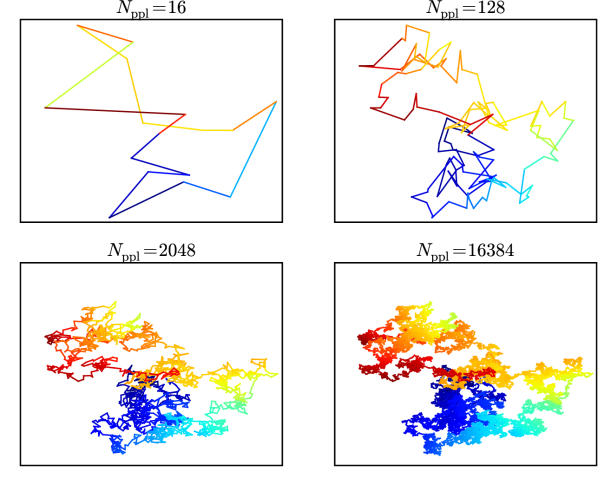
Figure 1: A single discrete worldline loop shown at several levels of discretization. The loops form fractal patterns and have a strong parallel with Brownian motion. The colour represents the phase of a particle travelling along the loop, and begins at dark blue, progresses in a random walk through yellow, and ends at dark red. The total flux through this particular worldline at $T=1$ and $B=B_{k}$ is about $0.08\pi/e$.

III Cylindrical Worldline Numerics

We now consider cylindrically symmetric external magnetic fields. In this case, we may simplify (6),

$$\frac{\Gamma^{(1)}_{\mathrm{ferm}}}{TL_{z}} = \frac{1}{4\pi}\int_{0}^{\infty}\rho_{\mathrm{cm}}\biggr{[}\int_{0}^{\infty}\frac{dT}{T^{3}}e^{-m^{2}T}\times$$

$$~{}~{}~{}~{}~{}~{}\left\{\langle W\rangle_{{\bf r}_{\mathrm{cm}}}-1-\frac{1}{3}(eB_{\mathrm{cm}}T)^{2}\right\}\biggr{]}d\rho.$$

III.1 Cylindrical Magnetic Fields

We have ${\bf B}=B(\rho)$${\bf\hat{z}}$ with

$$B(\rho)=\frac{A_{\phi}(\rho)}{\rho}+\frac{dA_{\phi}(\rho)}{d\rho}$$ (13)

if we make the gauge choice that $A_{0}=A_{\rho}=A_{z}=0$.

We begin by considering $A_{\phi}(\rho)$ in the form

$$A_{\phi}(\rho)=\frac{F}{2\pi\rho}f_{\lambda}(\rho)$$ (14)

so that

$$B_{z}(\rho)=\frac{F}{2\pi\rho}\frac{df_{\lambda}(\rho)}{d\rho}$$ (15)

and the total flux is

$$\Phi=F(f_{\lambda}(L_{\rho})-f_{\lambda}(0)).$$ (16)

It is convenient to express the flux in units of $\frac{2\pi}{e}$ and define a dimensionless quantity

$$\mathcal{F}=\frac{e}{2\pi}F.$$ (17)

III.2 Wilson Loop

The quantity inside the angled brackets in equation (6) is a gauge invariant observable called a Wilson loop. We note that the proper time integral provides a natural path ordering for this operator. The Wilson loop expectation value is

$$\langle W\rangle_{{\bf r}_{\mathrm{cm}}}\!\!=\biggl{\langle}e^{ie\int_{0}^{T}d\tau{\bf A}({\bf r}_{\mathrm{cm}}+{\bf r}(\tau))\cdot\dot{{\bf r}}}\frac{1}{4}\mathrm{tr}e^{\frac{e}{2}\int_{0}^{T}d\tau\sigma_{\mu\nu}F_{\mu\nu}({\bf r}_{\mathrm{cm}}+{\bf r}(\tau))}\biggr{\rangle}_{{\bf r}_{\mathrm{cm}}}\!\!\!\!\!\!\!\!,$$ (18)

which we look at as a product between a scalar part ($e^{ie\int_{0}^{T}d\tau{\bf A}({\bf r}_{\mathrm{cm}}+{\bf r}(\tau))\cdot\dot{{\bf r}}}$) and a fermionic part ($\frac{1}{4}\mathrm{tr}e^{\frac{e}{2}\int_{0}^{T}d\tau\sigma_{\mu\nu}F_{\mu\nu}({\bf r}_{\mathrm{cm}}+{\bf r}(\tau))}$).

III.2.1 Scalar Part

In a magnetic field, the scalar part is related to the flux through the loop, $\Phi_{B}$, by Stokes theorem:

$$e^{ie\int_{0}^{T}d\tau{\bf A}\cdot\dot{{\bf r}}} = e^{ie\oint{\bf A}\cdot d{\bf r}}=e^{ie\int_{{\bf\Sigma}}{\bf\nabla}\times{\bf A}\cdot d{\bf\Sigma}}$$ (19)

$$= e^{ie\int_{{\bf\Sigma}}{\bf B}d{\bf\Sigma}}=e^{ie\Phi_{B}}.$$ (20)

Consequently, this factor accounts for the Aharonov-Bohm phase acquired by particles in the loop.

The loop discretization results in the following approximation of the scalar integral:

$$\oint{\bf A}({\bf r})\cdot d{\bf r}=\sum_{i=1}^{N_{\mathrm{ppl}}}\int_{{\bf r}^{i}}^{{\bf r}^{i+1}}{\bf A}({\bf r})\cdot d{\bf r}.$$ (21)

Using a linear parameterization of the positions, the line integrals are

$$\int_{{\bf r}^{i}}^{{\bf r}^{i+1}}{\bf A}({\bf r})\cdot d{\bf r}=\int_{0}^{1}dt{\bf A}({\bf r}(t))\cdot({\bf r}^{i+1}-{\bf r}^{i}).$$ (22)

Using the same gauge choice outlined above (${\bf A}=A_{\phi}\hat{\phi}$), we may write

$${\bf A}({\bf r}(t))=\frac{\mathcal{F}}{e\rho^{2}}f_{\lambda}(\rho^{2})(-y,x,0),$$ (23)

where we have chosen $f_{\lambda}(\rho^{2})$ to depend on $\rho^{2}$ instead of $\rho$ to simplify some expressions and to avoid taking many costly square roots in the worldline numerics. We then have

$$\int_{{\bf r}^{i}}^{{\bf r}^{i+1}}{\bf A}({\bf r})\cdot d{\bf r}=\mathcal{F}(x^{i}y^{i+1}-y^{i}x^{i+1})\int_{0}^{1}dt\frac{f_{\lambda}(\rho_{i}^{2}(t))}{\rho_{i}^{2}(t)}.$$ (24)

The linear interpolation in Cartesian coordinates gives

$$\rho_{i}^{2}(t)=A_{i}+2B_{i}t+C_{i}t^{2},$$ (25)

where

$$A_{i} = (x^{i})^{2}+(y^{i})^{2}$$ (26)

$$B_{i} = x^{i}(x^{i+1}-x^{i})+y^{i}(y^{i+1}-y^{i})$$ (27)

$$C_{i} = (x^{i+1}-x^{i})^{2}+(y^{i+1}-y^{i})^{2}.$$ (28)

In performing the integrals along the straight lines connecting each discretized loop point, we are in danger of violating gauge invariance. If these integrals can be performed analytically, than gauge invariance is preserved exactly. However, in general, we wish to compute these integrals numerically. In this case, gauge invariance is no longer guaranteed, but can be preserved to any numerical precision that’s desired.

III.2.2 Fermion Part

For fermions, the Wilson loop is modified by a factor,

$$W^{\mathrm{ferm.}} = \frac{1}{4}\mathrm{tr}\left(e^{\frac{1}{2}e\int_{0}^{T}d\tau\sigma_{\mu\nu}F^{\mu\nu}}\right)$$ (29)

$$= \frac{1}{4}\mathrm{tr}\left(e^{\sigma_{xy}e\int_{0}^{T}d\tau B\left(x(\tau)\right)}\right)$$ (30)

$$= \cosh{\left(e\int_{0}^{T}d\tau B\left(x(\tau)\right)\right)}$$ (31)

$$= \cosh{\left(2\mathcal{F}\int_{0}^{T}d\tau f^{\prime}_{\lambda}(\rho^{2}(\tau))\right)},$$ (32)

where we have used the relation

$$eB=2\mathcal{F}\frac{df_{\lambda}(\rho^{2})}{d\rho^{2}}=2\mathcal{F}f^{\prime}_{\lambda}(\rho^{2}).$$ (33)

This factor represents an additional contribution to the action because of the spin interaction with the magnetic field. Classically, for a particle with a magnetic moment ${\bf\mu}$ travelling through a magnetic field in a time $T$, the action is modified by a term given by

$$\Gamma^{0}_{\mathrm{spin}}=\int_{0}^{T}{\bf\mu}\cdot{\bf B}({\bf x}(\tau))d\tau.$$ (34)

The magnetic moment is related to the electron spin ${\bf\mu}=g\left(\frac{e}{2m}\right){\bf\sigma}$, so we see that the integral in the above quantum fermion factor is very closely related to the classical action associated with transporting a magnetic moment through a magnetic field:

$$\Gamma^{0}_{\mathrm{spin}}=g\left(\frac{e}{2m}\right)\sigma_{xy}\int_{0}^{T}B_{z}(x(\tau))d\tau.$$ (35)

Qualitatively, we could write

$$W^{\mathrm{ferm}}\sim\cosh{\left(\Gamma^{0}_{\mathrm{spin}}\right)}.$$ (36)

As a possibly useful aside, we may want to express the integral in terms of $f_{\lambda}(\rho^{2})$ instead of its derivative. We can do this by integrating by parts:

$$\int_{0}^{T}d\tau f^{\prime}_{\lambda}(\rho^{2}(\tau)) = \frac{T}{N_{\mathrm{ppl}}}\sum_{i=1}^{N_{\mathrm{ppl}}}\int_{0}^{1}dtf^{\prime}_{\lambda}(\rho^{2}_{i}(\tau))$$ (38)

$$= \frac{T}{N_{\mathrm{ppl}}}\sum_{i=1}^{N_{\mathrm{ppl}}}\biggr{[}\frac{f_{\lambda}(\rho^{2}_{i}(t))}{2(B_{i}+C_{i}t)}\biggr{|}^{t=1}_{t=0}$$

$$+\frac{C_{i}}{2}\!\!\int_{0}^{1}\!\!\!\!\frac{f_{\lambda}(\rho^{2}_{i}(t))}{(B_{i}+C_{i}t)^{2}}dt\biggr{]}$$

$$= \frac{T}{N_{\mathrm{ppl}}}\sum_{i=1}^{N_{\mathrm{ppl}}}\frac{C_{i}}{2}\!\!\int_{0}^{1}\!\!\!\!\frac{f_{\lambda}(\rho^{2}_{i}(t))}{(B_{i}+C_{i}t)^{2}}dt,$$ (39)

with $\rho_{i}^{2}(t)$ given by equations (25) to (28). The second equality is obtained from integration-by-parts. In the third equality, we use the loop sum to cancel the boundary terms in pairs:

$$W^{\mathrm{ferm.}}=\cosh{\left(\frac{\mathcal{F}T}{N_{\mathrm{ppl}}}\sum_{i=1}^{N_{\mathrm{ppl}}}C_{i}\int_{0}^{1}dt\frac{f_{\lambda}(\rho^{2}_{i}(t))}{(B_{i}+C_{i}t)^{2}}\right)}.$$ (40)

In most cases, one would use equation (32) to compute the fermion factor of the Wilson loop. However, equation (40) may be useful in cases where $f^{\prime}_{\lambda}(\rho^{2}(\tau))$ is not known or is difficult to compute.

III.3 Renormalization

The field strength renormalization counter-terms result from the small $T$ behaviour of the worldline integrand. In the limit where $T$ is very small, the worldline loops are very localized around their center of mass. So, we may approximate their contribution as being that of a constant field with value ${\bf A}({\bf r}_{\mathrm{cm}})$. Specifically, we require that the field change slowly on the length scale defined by $\sqrt{T}$. This condition on $T$ can be written

$$T\ll\left|\frac{m^{2}}{eB^{\prime}(\rho^{2})}\right|=\left|\frac{m^{2}}{2\mathcal{F}f^{\prime\prime}_{\lambda}(\rho^{2}_{\mathrm{cm}})}\right|.$$ (41)

When this limit is satisfied, we may use the exact expressions for the constant field Wilson loops to determine the small $T$ behaviour of the integrands and the corresponding counter terms.

The Wilson loop averages for constant magnetic fields in scalar and fermionic QED are

$$\langle W\rangle_{\mathrm{ferm}}=eBT\coth{(eBT)}$$ (42)

and

$$\langle W\rangle_{\mathrm{scal}}=\frac{eBT}{\sinh{(eBT)}}.$$ (43)

Therefore, the integrand for fermionic QED in the limit of small $T$ is

$$I_{\mathrm{ferm}}(T) = \frac{e^{-m^{2}T}}{T^{3}}\left[eB({\bf r}_{cm})T\coth{(eB({\bf r}_{cm})T)}-1-\frac{e^{2}}{3}B^{2}({\bf r}_{cm})T^{2}\right]$$ (44)

$$\approx -\frac{(eB)^{4}T}{45}+\frac{1}{45}(eB)^{4}m^{2}T^{2}+\left(\frac{2(eB)^{6}}{945}-\frac{(eB)^{4}m^{4}}{90}\right)T^{3}+\frac{(7(eB)^{4}m^{6}-4(eB)^{6}m^{2})T^{4}}{1890}+O(T^{5}).$$

For scalar QED we have

$$I_{\mathrm{scal}}(T) = \frac{e^{-m^{2}T}}{T^{3}}\left[\frac{eB({\bf r}_{cm})T}{\sinh{(eB({\bf r}_{cm})T)}}-1+\frac{1}{6}(eB)^{2}({\bf r}_{cm})T^{2}\right]$$ (45)

$$\approx \frac{7(eB)^{4}T}{360}-\frac{7(eB)^{4}m^{2}T^{2}}{360}+\frac{(147(eB)^{4}m^{4}-31(eB)^{6})T^{3}}{15120}+\frac{(31(eB)^{6}m^{2}-49(eB)^{4}m^{6})T^{4}}{15120}+O(T^{5}).$$

Beyond providing the renormalization conditions, these expansions can be used in the small $T$ regime to avoid a problem with the Wilson loop uncertainties in this region. Consider the uncertainty in the integrand arising from the uncertainty in the Wilson loop:

$$\delta I(T)=\frac{\partial I}{\partial W}\delta W=\frac{e^{-m^{2}T}}{T^{3}}\delta W.$$ (46)

In this case, even though we can compute the Wilson loops for small $T$ precisely, even a small uncertainty is magnified by a divergent factor when computing the integrand for small values of $T$. So, in order to perform the integral, we must replace the small $T$ behaviour of the integrand with the above expansions (44) and (45). Our worldline integral then proceeds by analytically computing the integral for the small $T$ expansion up to some small value, $a$, and adding this to the remaining part of the integral MoyaertsLaurent:2004 :

$$\int_{0}^{\infty}I(T)dT=\underbrace{\int_{0}^{a}I(T)dT}_{\mathrm{small~{}T}}+\underbrace{\int_{a}^{\infty}I(T)dT}_{\mathrm{worldline~{}numerics}}.$$ (47)

Because this normalization procedure uses the constant field expressions for small values of $T$, this scheme introduces a small systematic uncertainty. To improve on the method outlined here, the derivatives of the background field can be accounted for by using the analytic forms of the heat kernel expansion to perform the renormalization Gies:2001tj .

IV Uncertainty analysis in worldline numerics

So far in the worldline numerics literature, the discussions of uncertainty analysis have been unfortunately brief. It has been suggested that the standard deviation of the worldlines provides a good measure of the statistical error in the worldline method Gies:2001zp ; Gies:2001tj . However, the distributions produced by the worldline ensemble are highly non-Gaussian (see figure 5), and therefore the standard error in the mean is not a good measure of the uncertainties involved. Furthermore, the use of the same worldline ensemble to compute the Wilson loop multiple times in an integral results in strongly correlated uncertainties. Thus, propagating uncertainties through integrals can be computationally expensive due to the complexity of computing correlation coefficients.

The error bars on worldline calculations impact the conclusions that can be drawn from calculations, and also have important implications for the fermion problem, which limits the domain of applicability of the technique (see section IV.3). It is therefore important that the error analysis is done thoughtfully and transparently. The purpose of this chapter is to contribute a more thorough discussion of uncertainty analysis in the worldline numerics technique to the literature in hopes of avoiding any confusion associated with the above-mentioned subtleties.

There are two sources of uncertainty in the worldline technique: the discretization error in treating each continuous worldline as a set of discrete points, and the statistical error of sampling a finite number of possible worldlines from a distribution. In this section, we discuss each of these sources of uncertainty.

IV.1 Estimating the Discretization Uncertainties

The discretization error arising from the integral over $\tau$ in the exponent of each Wilson loop (see equation (18)) is difficult to estimate since any number of loops could be represented by each choice of discrete points. The general strategy is to make this estimation by computing the Wilson loop using several different numbers of points per worldline and observing the convergence properties.

The specific procedure adopted for this work involves dividing each discrete worldline into several worldlines with varying levels of discretization. Since we are using the d-loop method for generating the worldlines (section II.1), a $\frac{N_{\mathrm{ppl}}}{2}$ sub-loop consisting of every other point will be guaranteed to contain the prescribed distribution of velocities.

To look at the convergence for the loop discretization, each worldline is divided into three groups. One group of $\frac{N_{\mathrm{ppl}}}{2}$ points, and two groups of $\frac{N_{\mathrm{ppl}}}{4}$. This permits us to compute the average holonomy factors at three levels of discretization:

$$\langle W\rangle_{N_{\mathrm{ppl}}/4}=\langle e^{\frac{i}{2}\triangle}e^{\frac{i}{2}\Box}\rangle,$$ (48)

$$\langle W\rangle_{N_{\mathrm{ppl}}/2}=\langle e^{i\circ}\rangle,$$ (49)

and

$$\langle W\rangle_{N_{\mathrm{ppl}}}=\langle e^{\frac{i}{2}\circ}e^{\frac{i}{4}\Box}e^{\frac{i}{4}\triangle}\rangle,$$ (50)

where the symbols $\circ$, $\Box$, and $\triangle$ denote the worldline integral, $\int_{0}^{T}d\tau A(x_{CM}+x(\tau))\cdot\dot{x}$, computed using the sub-worldlines depicted in figure 2.

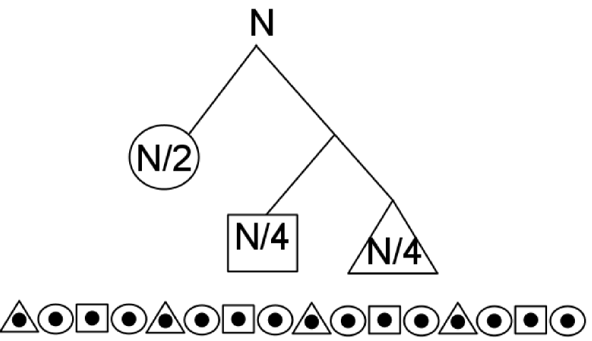
Figure 2: Diagram illustrating the division of a worldline into three smaller interleaved worldlines

We may put these factors into the equation of a parabola to extrapolate the result to an infinite number of points per line (see figure 3):

$$\langle W\rangle_{\infty}\approx\frac{8}{3}\langle W\rangle_{N_{\mathrm{ppl}}}-2\langle W\rangle_{N_{\mathrm{ppl}}/2}+\frac{1}{3}\langle W\rangle_{N_{\mathrm{ppl}}/4}.$$ (51)

So, we estimate the discretization uncertainty to be

$$\delta\langle W\rangle_{\infty}\approx|\langle W\rangle_{N_{\mathrm{ppl}}}-\langle W\rangle_{\infty}|.$$ (52)

Generally, the statistical uncertainties are the limitation in the precision of the worldline numerics technique. Therefore, $N_{\mathrm{ppl}}$ should be chosen to be large enough that the discretization uncertainties are small relative to the statistical uncertainties.

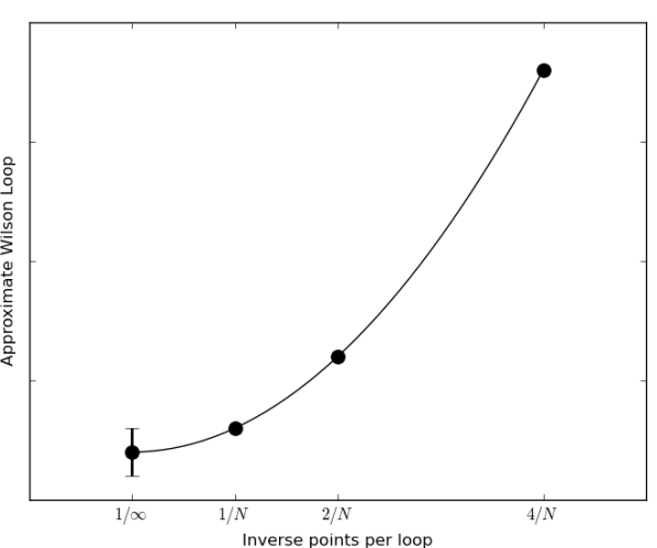
Figure 3: This plot illustrates the method used to extrapolate the Wilson loop to infinite points per loop and the uncertainty estimate in the approximation.

IV.2 Estimating the Statistical Uncertainties

We can gain a great deal of insight into the nature of the statistical uncertainties by examining the specific case of the uniform magnetic field since we know the exact solution in this case.

IV.2.1 The Worldline Ensemble Distribution is not Normal.

A reasonable first instinct for estimating the error bars is to use the standard error in the mean of the collection of individual worldlines:

$$\mathrm{SEM}(W)=\sqrt{\sum_{i=1}^{N_{l}}\frac{(W_{i}-\langle W\rangle)^{2}}{N_{l}(N_{l}-1)}}.$$ (53)

This approach has been promoted in early papers on worldline numerics Gies:2001zp ; Gies:2001tj . In figure 4, we have plotted the residuals and the corresponding error bars for several values of the proper time parameter, $T$. From this plot, it appears that the error bars are quite large in the sense that we appear to produce residuals which are considerably smaller than would be implied by the sizes of the error bars. This suggests that we have overestimated the size of the uncertainty.

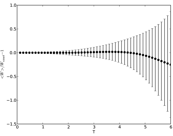
Figure 4: Residuals of worldline calculations and the corresponding standard errors in the mean. For reasons discussed in this section, these error bars overestimate the uncertainties involved.

We can see why this is the case by looking more closely at the distributions produced by the worldline technique. An exact expression for these distributions can be derived in the case of the constant magnetic field MoyaertsLaurent:2004 :

$$w(y) = \frac{W_{\mathrm{exact}}}{\sqrt{1-y^{2}}}\sum_{n=-\infty}^{\infty}\biggl{[}f(\arccos(y)+2n\pi)+$$ (54)

$$~{}~{}~{}~{}~{}~{}~{}~{}~{}~{}~{}~{}f(-\arccos(y)+2n\pi)\biggr{]}$$

with

$$f(\phi)=\frac{\pi}{4BT\cosh^{2}(\frac{\pi\phi}{2BT})}.$$ (55)

Figure 5 shows histograms of the worldline results along with the expected distributions. These distributions highlight a significant hurdle in assigning error bars to the results of worldline numerics.

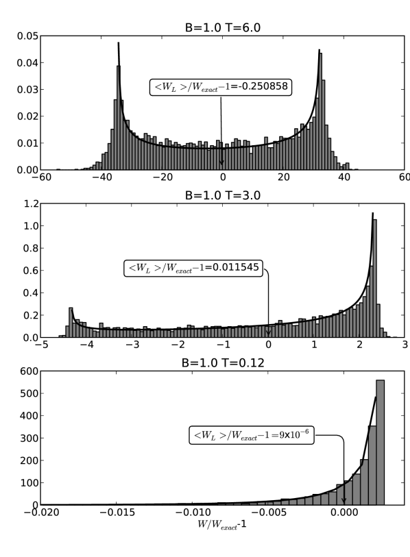
Figure 5: Histograms showing the worldline distributions of the residuals for three values of $T$ in the constant magnetic field case. Here, we are neglecting the fermion factor. The dark line represents the exact distribution computed using equation 54. The worldline means are indicated with an arrow, while the exact mean in each case is 0. There are 5120 worldlines in each histogram. The vertical axes are normalized to a total area of unity.

Due to their highly non-Gaussian nature, the standard error in the mean is not a good characterization of the distributions that are produced. We should not interpret each individual worldline as a measurement of the mean value of these distributions; for large values of $BT$, almost all of our worldlines will produce answers which are far away from the mean of the distribution. This means that the variance of the distribution will be very large, even though our ability to determine the mean of the distribution is relatively precise because of the increasing symmetry about the mean as $T$ becomes large.

IV.2.2 Correlations between Wilson Loops

Typically, numerical integration is performed by replacing the integral with a sum over a finite set of points from the integrand. We will begin the present discussion by considering the uncertainty in adding together two points (labelled $i$ and $j$) in our integral over $T$. Two terms of the sum representing the numerical integral will involve a function of $T$ times the two Wilson loop factors,

$$I=g(T_{i})\langle W(T_{i})\rangle+g(T_{j})\langle W(T_{j})\rangle$$ (56)

with an uncertainty given by

$$\delta I = \left|\frac{\partial I}{\partial\langle W(T_{i})\rangle}\right|^{2}(\delta\langle W(T_{i})\rangle)^{2}$$ (58)

$$~{}~{}+\left|\frac{\partial I}{\partial\langle W(T_{j})\rangle}\right|^{2}(\delta\langle W(T_{j})\rangle)^{2}$$

$$~{}~{}+2\left|\frac{\partial I}{\partial\langle W(T_{i})\rangle}\frac{\partial I}{\partial\langle W(T_{j})\rangle}\right|\times$$

$$~{}~{}\rho_{ij}(\delta\langle W(T_{i})\rangle)(\delta\langle W(T_{j})\rangle)$$

$$= g(T_{i})^{2}(\delta\langle W(T_{i})\rangle)^{2}+g(T_{j})^{2}(\delta\langle W(T_{j})\rangle)^{2}+$$

$$~{}2\left|g(T_{i})g(T_{j})\right|\rho_{ij}(\delta\langle W(T_{i})\rangle)(\delta\langle W(T_{j})\rangle)$$

and the correlation coefficient $\rho_{ij}$ given by

$$\rho_{ij}=\frac{\langle(W(T_{i})-\langle W(T_{i})\rangle)(W(T_{j})-\langle W(T_{j})\rangle)\rangle}{\sqrt{(W(T_{i})-\langle W(T_{i})\rangle)^{2}}\sqrt{(W(T_{j})-\langle W(T_{j})\rangle)^{2}}}.$$ (59)

The final term in the error propagation equation takes into account correlations between the random variables $W(T_{i})$ and $W(T_{j})$. Often in a Monte Carlo computation, one can treat each evaluation of the integrand as independent, and neglect the uncertainty term involving the correlation coefficient. However, in worldline numerics, the evaluations are related because the same worldline ensemble is reused for each evaluation of the integrand. The correlations are significant (see figure 6), and this term can’t be neglected. Computing each correlation coefficient takes a time proportional to the square of the number of worldlines. Therefore, it may be computationally expensive to formally propagate uncertainties through an integral.

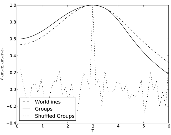
Figure 6: Correlation coefficients, equation (59), between $\langle W(T)\rangle$ and $\langle W(T=3)\rangle$ computed using individual worldlines, groups of worldlines, and shuffled groups of worldlines.

The point-to-point correlations were originally pointed out by Gies and Langfeld who addressed the problem by updating (but not replacing or regenerating) the loop ensemble in between each evaluation of the Wilson loop average Gies:2001zp . This may be a good way of addressing the problem. However, in the following section, we promote a method which can bypass the difficulties presented by the correlations by treating the worldlines as a collection of worldline groups.

IV.2.3 Grouping Worldlines

Both of the problems explained in the previous two subsections can be overcome by creating groups of worldline loops within the ensemble. Each group of worldlines then makes a statistically independent measurement of the Wilson loop average for that group. The statistics between the groups of measurements are normally distributed, and so the uncertainty is the standard error in the mean of the ensemble of groups (in contrast to the ensemble of worldlines).

For example, if we divide the $N_{l}$ worldlines into $N_{G}$ groups of $N_{l}/N_{G}$ worldlines each, we can compute a mean for each group:

$$\langle W\rangle_{G_{j}}=\frac{N_{G}}{N_{l}}\sum_{i=1}^{N_{l}/N_{G}}W_{i}.$$ (60)

Provided each group contains the same number of worldlines, the average of the Wilson loop is unaffected by this grouping:

$$\langle W\rangle = \frac{1}{N_{G}}\sum_{j=1}^{N_{G}}\langle W\rangle_{G_{j}}$$ (61)

$$= \frac{1}{N_{l}}\sum_{i=1}^{N_{l}}W_{i}.$$ (62)

However, the uncertainty is the standard error in the mean of the groups,

$$\delta\langle W\rangle=\sqrt{\sum_{i=1}^{N_{G}}\frac{(\langle W\rangle_{G_{i}}-\langle W\rangle)^{2}}{N_{G}(N_{G}-1)}}.$$ (63)

Because the worldlines are unrelated to one another, the choice of how to group them to compute a particular Wilson loop average is arbitrary. For example, the simplest choice is to group the loops by the order they were generated, so that a particular group number, $i$, contains worldlines $iN_{l}/N_{G}$ through $(i+1)N_{l}/N_{G}-1$. Of course, if the same worldline groupings are used to compute different Wilson loop averages, they will still be correlated. We will discuss this problem in a moment.

The basic claim of the worldline technique is that the mean of the worldline distribution approximates the holonomy factor. However, from the distributions in figure 5, we can see that the individual worldlines themselves do not approximate the holonomy factor. So, we should not think of an individual worldline as an estimator of the mean of the distribution. Thus, a resampling technique is required to determine the precision of our statistics. We can think of each group of worldlines as making an independent measurement of the mean of a distribution. As expected, the groups of worldlines produce a more Gaussian-like distribution (see figure 7), and so the standard error of the groups is a sensible measure of the uncertainty in the Wilson loop value.

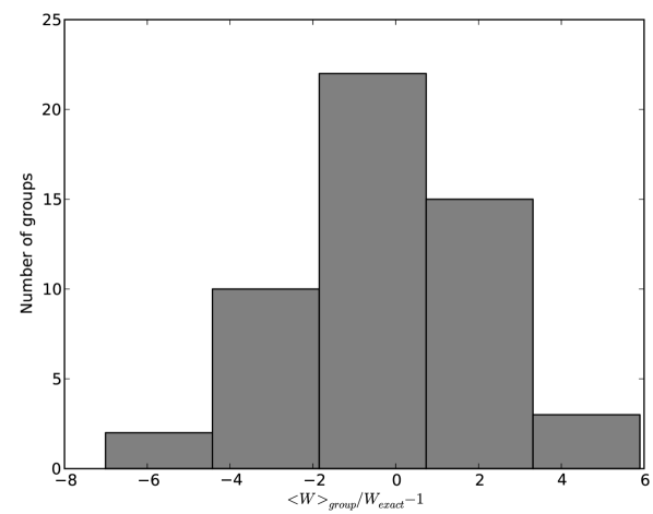
Figure 7: The histogram demonstrating the precision with which we can reproduce measurements of the mean using different groups of 100 worldlines at $BT=6.0$. In this case, the distribution is Gaussian-like and meaningful error bars can be placed on our measurement of the mean.

We find that the error bars are about one-third as large as those determined from the standard error in the mean of the individual worldlines, and the smaller error bars better characterize the size of the residuals in the constant field case (see figure 8). The strategy of using subsets of the available data to determine error bars is called jackknifing. Several previous papers on worldline numerics have mentioned using jackknife analysis to determine the uncertainties, but without an explanation of the motivations or the procedure employed 2005PhRvD..72f5001G ; PhysRevLett.96.220401 ; Dunne:2009zz ; PhysRevD.84.065035 .

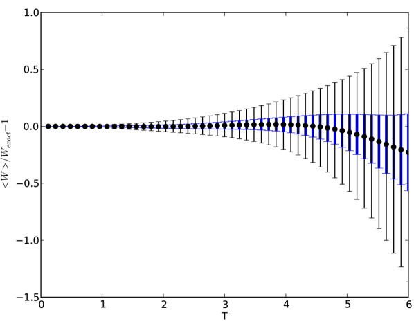
Figure 8: The residuals of the Wilson loops for a constant magnetic field showing the standard error in the mean (thin error bars) and the uncertainty in determining the mean (thick blue error bars). The standard error in the mean overestimates the uncertainty by more than a factor of 3 at each value of $T$.

The grouping of worldlines alone does not address the problem of correlations between different evaluations of the integrands. Figure 6 shows that the uncertainties for groups of worldlines are also correlated between different points of the integrand. However, the worldline grouping does provide a tool for bypassing the problem. One possible strategy is to randomize how worldlines are assigned to groups between each evaluation of the integrand. This produces a considerable reduction in the correlations, as is shown in figure 6. Then, errors can be propagated through the integrals by neglecting the correlation terms. Another strategy is to separately compute the integrals for each group of worldlines, and then consider the statistics of the final product to determine the error bars. This second strategy is the one adopted for the work presented in this paper. Grouping in this way reduces the amount of data which must be propagated through the integrals by a factor of the group size compared to a delete-1 jackknife scheme, for example. In general, the error bars quoted in the remainder of this paper are obtained by computing the standard error in the mean of groups of worldlines.

IV.3 Uncertainties and the Fermion Problem

The fermion problem of worldline numerics is a name given to an enhancement of the uncertainties at large $T$ Gies:2001zp ; MoyaertsLaurent:2004 . It should not be confused with the fermion-doubling problem associated with lattice methods. In a constant magnetic field, the scalar portion of the calculation produces a factor of $\frac{BT}{\sinh{(BT)}}$, while the fermion portion of the calculation produces an additional factor $\cosh{(BT)}$. Physically, this contribution arises as a result of the energy required to transport the electron’s magnetic moment around the worldline loop. At large values of $T$, we require subtle cancellation between huge values produced by the fermion portion with tiny values produced by the scalar portion. However, for large $T$, the scalar portion acquires large relative uncertainties which make the computation of large $T$ contributions to the integral very imprecise.

This can be easily understood by examining the worldline distributions shown in figure 5. Recall that the scalar Wilson loop average for these histograms is given by the flux in the loop, $\Phi_{B}$:

$$\langle W\rangle=\left<\exp{\left(ie\int_{0}^{T}d\tau{\bf A}({\bf x}_{\mathrm{cm}}+{\bf x}(\tau))\cdot d{\bf x}(\tau)\right)}\right>=\left<e^{ie\Phi_{B}}\right>.$$ (64)

For constant fields, the flux through the worldline loops obeys the distribution function MoyaertsLaurent:2004

$$f(\Phi_{B})=\frac{\pi}{4BT\cosh^{2}\left(\frac{\pi\Phi_{B}}{2BT}\right)}.$$ (65)

For small values of $T$, the worldline loops are small and the amount of flux through the loop is correspondingly small. Therefore, the flux for small loops is narrowly distributed about $\Phi_{B}=0$. Since zero maximizes the Wilson loop ($e^{i0}=1$), this explains the enhancement to the right of the distribution for small values of $T$. As $T$ is increased, the flux through any given worldline becomes very large and the distribution of the flux becomes very broad. For very large $T$, the width of the distribution is many factors of $2\pi/e$. Then, the phase ($e\Phi_{B}\mod{2\pi}$) is nearly uniformly distributed, and the Wilson loop distribution reproduces the Chebyshev distribution (i.e. the distribution obtained from projecting uniformly distributed points on the unit circle onto the horizontal axis),

$$\lim_{T\to\infty}w(y)=\frac{1}{\pi\sqrt{1-y^{2}}}.$$ (66)

The mean of the Chebyshev distribution is zero due to its symmetry. However, this symmetry is not realized precisely unless we use a very large number of loops. Since the width of the distribution is already 100$\times$ the value of the mean at $T=6$, any numerical asymmetries in the distribution result in very large relative uncertainties of the scalar portion. Because of these uncertainties, the large contribution from the fermion factor are not cancelled precisely.

This problem makes it very difficult to compute the fermionic effective action unless the fields are well localized MoyaertsLaurent:2004 . For example, the fermionic factor for non-homogeneous magnetic fields oriented along the z-direction is

$$\cosh{\left(e\int_{0}^{T}d\tau B(x(\tau))\right)}.$$ (67)

For a homogeneous field, this function grows exponentially with $T$ and is cancelled by the exponentially vanishing scalar Wilson loop. For a localized field, the worldline loops are very large for large values of $T$, and they primarily explore regions far from the field. Thus, the fermionic factor grows more slowly in localized fields, and is more easily cancelled by the rapidly vanishing scalar part.

In this section, we have identified two important considerations in determining the uncertainties associated with worldline numerics computations. Firstly, the computed points within the integrals over proper time, $T$, or center of mass, ${\bf x}_{\mathrm{cm}}$, are highly correlated because one typically reuses the same ensemble of worldlines to compute each point. Secondly, the statistics of the worldlines are not normally distributed and each individual worldline in the ensemble may produce a result which is very far from the mean value. So, in determining the uncertainties in the worldline numerics technique, one should consider how precisely the mean of the ensemble can be measured from the ensemble and this is not necessarily given by the standard error in the mean.

These issues can be addressed simultaneously using a scheme where the worldlines from the ensemble are placed into groups, and the effective action or the effective action density is evaluated separately for each group. The uncertainties can then be determined by the statistics of the groups. This scheme is less computationally intensive than a delete-1 jackknife approach because less data (by a factor of the group size) needs to be propagated through the integrals. It is also less computationally intensive than propagating the uncertainties through the numerical integrals because it avoids the computation of numerous correlation coefficients.

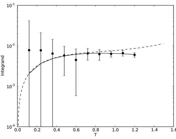
Figure 9: The small $T$ behaviour of worldline numerics. The data points represent the numerical results, where the error bars are determined from the jackknife analysis described in chapter IV. The solid line represents the exact solution while the dotted line represents the small $T$ expansion of the exact solution. Note the amplification of the uncertainties.

V Computing an Effective Action

The ensemble average in the effective action is simply the sum over the contributions from each worldline loop, divided by the number of loops in the ensemble. Since the computation of each loop is independent of the other loops, the ensemble average may be straightforwardly parallelized by generating separate processes to compute the contribution from each loop. For this parallelization, four Nvidia Tesla C1060 GPU were used through the CUDA parallel programming framework. Because GPU can spawn thousands of parallel processing threads with much less computational overhead than an MPI cluster, they excel at handling a very large number of parallel threads, although the clock speed is slower and fewer memory resources are typically available. In contrast, parallel computing on a cluster using CPU tends to have a much higher speed per thread, but there are typically fewer threads available. The worldline technique is exceedingly parallelizable, and it is a straightforward matter to divide the task into thousands or tens of thousands of parallel threads. In this case, one should expect excellent performance from a GPU over a parallel CPU implementation, unless thousands of CPU are available for the program. The GPU architecture has recently been used by another group for computing Casimir forces using worldline numerics 2011arXiv1110.5936A . Figure 10 illustrates the co-processing and parallelization scheme used here for the worldline numerics.

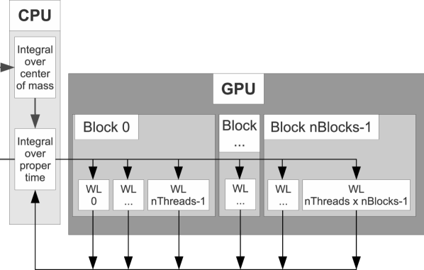
Figure 10: The CPU manages the loops which compute the integrals over center of mass and proper time. For each proper time integral, we require the results from a large number of individual worldlines. The GPU is used to compute the integral over each worldline in parallel, and the results are returned to the CPU for use in the effective action calculation.

.

In an informal test, a Wilson loop average was computed using an ensemble of 5000 loops in 4.7553 seconds using a serial implementation while the GPU performed the same calculation in 0.001315 seconds using a CUDA implementation. A parallel CPU code would require a cluster with thousands of cores to achieve a similar speed, even if we assume linear (ideal) speed-up. So, for worldline numerics computations, a relatively inexpensive GPU can be expected to outperform a small or mid-sized cluster. This increase in computation speed has enabled the detailed parameter searches discussed in this dissertation.

Of course, there are also trade-offs from using the GPU architecture with the worldline numerics technique. The most significant of these is the limited availability of memory on the device. A GPU device provides only a few GB of global memory (4GB on the Tesla C1060). This limit forces compromises between the number of points-per-loop and the number of loops to keep the total size of the loop cloud data small. The limited availability of memory resources also limits the number of threads which can be executed concurrently on the device. Because of the overhead associated with transferring data to and from the device, the advantages of a GPU over a CPU cluster are most pronounced on problems which can be divided into several hundred or thousands of processes. Therefore, the GPU may not offer great performance advantages for a small number of loops. Finally, there is some additional complexity involved in programming for the GPU in terms of learning specialized libraries and memory management on the device. This means that the code may take longer to develop and there may be a learning curve for researchers. However, this problem is not much more pronounced with GPU programming than with other parallelization strategies.

Once the ensemble average of the Wilson loop has been computed, computing the effective action is a straightforward matter of performing numerical integrals. The effective action density is computed by performing the integration over proper time, $T$. Then, the effective action is computed by performing a spacetime integral over the loop ensemble center of mass. In all cases where a numerical integral was performed, Simpson’s method was used burden2001numerical . Integrals from 0 to $\infty$ were mapped to the interval $[0,1]$ using substitutions of the form $x=\frac{1}{1+T/T_{\mathrm{max}}}$, where $T_{\mathrm{max}}$ sets the scale for the peak of the integrand. In the constant field case, for the integral over proper time, we expect $T_{\mathrm{max}}\sim 3/(eB)$ for large fields and $T_{\mathrm{max}}\sim 1$ for fields of a few times critical or smaller. In section IV, we presented a detailed discussion of how the statistical and discretization uncertainties can be computed in this technique.

In this implementation, the numerical integrals are done using a serial CPU computation. This serial portion of the algorithm tends to limit the speedup that can be achieved with the large number of parallel threads on the GPU device. However, an important benefit of the large number of threads available on the GPU is that the number of worldlines in the ensemble can be increased without limit, as long as more threads are available, without significantly increasing the computation time. If perfect occupancy could be achieved on a Tesla C1060 device, an ensemble of up to 30,720 worldlines could be computed concurrently. Thus, the GPU provides an excellent architecture for improving the statistical uncertainties. Additionally, there is room for further optimization of the algorithm by parallelizing the serial portions of the algorithm to achieve a greater speedup.

More details about implementing this algorithm on the CUDA architecture can be found in appendix A. A listing of the CUDA worldline numerics code appears in appendix of 2012PhDT……..21M .

VI Verification and Validation

The worldline numerics software can be validated and verified by making sure that it produces the correct results where the derivative expansion is a good approximation, and that the results are consistent with previous numerical calculations of flux tube effective actions. For this reason, the validation was done primarily with flux tubes with a profile defined by the function

$$f_{\lambda}(\rho^{2})=\frac{\rho^{2}}{(\lambda^{2}+\rho^{2})}.$$ (68)

For large values of $\lambda$, this function varies slowly on the Compton wavelength scale, and so the derivative expansion is a good approximation. Also, flux tubes with this profile were studied previously using worldline numerics Moyaerts:2003ts ; MoyaertsLaurent:2004 .

Among the results presented in MoyaertsLaurent:2004 is a comparison of the derivative expansion and worldline numerics for this magnetic field configuration. The result is that the next-to-leading-order term in the derivative expansion is only a small correction to the the leading-order term for $\lambda\gg\lambda_{e}$, where the derivative expansion is a good approximation. The derivative expansion breaks down before it reaches its formal validity limits at $\lambda\sim\lambda_{e}$. For this reason, we will simply focus on the leading order derivative expansion (which we call the LCF approximation). The effective action of QED in the LCF approximation is given in cylindrical symmetry by

$$\Gamma^{(1)}_{\mathrm{ferm}} = \frac{1}{4\pi}\int_{0}^{\infty}dT\int_{0}^{\infty}\rho_{\mathrm{cm}}d\rho_{\mathrm{cm}}\frac{e^{-m^{2}T}}{T^{3}}\times$$

$$\biggl{\{}eB(\rho_{\mathrm{cm}})T\coth{(eB(\rho_{\mathrm{cm}})T)}$$

$$-1-\frac{1}{3}(eB(\rho_{\mathrm{cm}})T)^{2}\biggr{\}}.$$

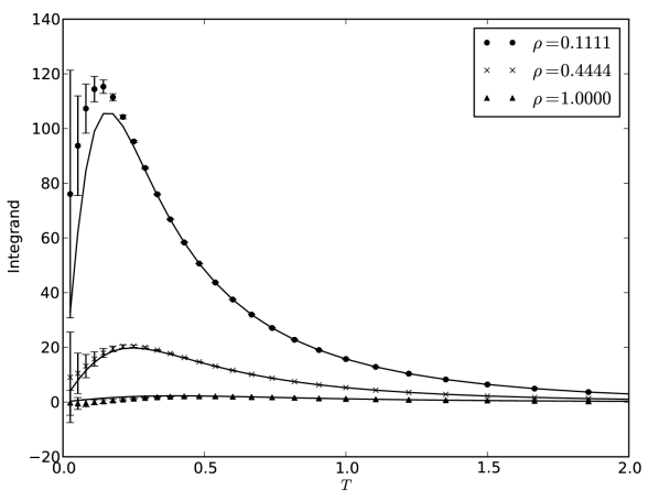
Figure 11: The integrand of the proper time, $T$, integral for three different values of the radial coordinate, $\rho$ for a $\lambda=1$ flux tube. The solid lines represent the zeroth-order derivative expansion, which, as expected, is a good approximation until $\rho$ becomes too small.

Figure 11 shows a comparison between the proper time integrand,

$$\frac{e^{-m^{2}T}}{T^{3}}\left[\langle W\rangle_{{\bf r}_{\mathrm{cm}}}-1-\frac{1}{3}(eB_{\mathrm{cm}}T)^{2}\right],$$ (70)

and the LCF approximation result for a flux tube with $\lambda=\lambda_{e}$ and $\mathcal{F}=10$. In this case, the LCF approximation is only appropriate far from the center of the flux tube, where the field is not changing very rapidly. In the figure, we can begin to see the deviation from this approximation, which gets more pronounced closer to the center of the flux tube (smaller values of $\rho$).

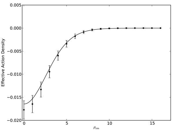
Figure 12: The fermion term of the effective action density as a function of the radial coordinate for a flux tube with width $\lambda=10\lambda_{e}$.

The effective action density for a slowly varying flux tube is plotted in figure 12 along with the LCF approximation. In this case, the LCF approximation agrees within the statistics of the worldline numerics.

VII Conclusions

In this paper, we have reviewed the worldline numerics numerical technique with a focus on computing the effective action of QED in non-homogeneous, cylindrically symmetric magnetic fields. The method uses a Monte Carlo generated ensemble of worldline loops to approximate a path integral in the worldline formalism. These worldline loops are generated using a simple algorithm and encode the information about the magnetic field by computing the flux through the loop and the action acquired from transporting a magnetic moment around the loop. This technique preserves Lorentz symmetry exactly and can preserve gauge symmetry up to any required precision.

We have discussed implementing this technique on GPU architecture using CUDA. The main advantage of this architecture is that it allows for a very large number of concurrent threads which can be utilized with very little overhead. In practice, this means that a large ensemble of worldlines can be computed concurrently, thus allowing for a considerable speedup over serial implementations, and allowing for the precision of the numerics to increase according to the number of threads available.

This work was supported by the Natural Sciences and Engineering Research Council of Canada, the Canadian Foundation for Innovation, the British Columbia Knowledge Development Fund. It has made used of the NASA ADS and arXiv.org.

*

Appendix A CUDAfication of Worldline Numerics

Our implementation of the worldline numerics technique used a “co-processing” (or heterogeneous) approach where the CPU and GPU are both used in unison to compute different aspects of the problem. The CPU was used for computing the spatial and proper-time integrals while the GPU was employed to compute the contributions to the Wilson Loop from each worldline in parallel for each value of $\rho_{\mathrm{cm}}$ and $T$. This meant that each time the integrand was to be computed, it could be computed thousands of times faster than on a serial implementation. A diagram illustrating the co-processing approach is shown in figure 10.

Code which runs on the GPU device must be implemented using specialized tools such as the CUDA-C programming language cudazone ; CUDAGuide3.2 . The CUDA language is an extension of the C programming language and compiles under a proprietary compiler, nvcc, which is based off of the GNU C compiler, gcc.

A.1 Overview of CUDA

CUDA programs make use of special functions, called kernel functions, which are executed many times in parallel. Each parallel thread executes a copy of the kernel function, and is provided with a unique identification number, threadIdx. threadIdx may be a one, two, or three-dimensional vector index, allowing the programmer to organize the threads logically according to the task.

A program may require many thousands of threads, which are organized into a series of organizational units called blocks. For example, the Tesla C1060 GPU allows for up to 1024 threads per block. These blocks are further organized into a one or two-dimensional structure called the grid. CUDA allows for communication between threads within a block, but each block is required to execute independently of other blocks.

CUDA uses a programming model in which the GPU and CPU share processing responsibilities. The CPU runs a host process which may call different kernel functions many times over during its lifetime. When the host process encounters a kernel function call, the CUDA device takes control of the processing by spawning the designated number of threads and blocks to evaluate the kernel function many times in parallel. After the kernel function has executed, control is returned to the host process which may then copy the data from the device to use in further computations.

The GPU device has separate memory from that used by the CPU. In general, data must be copied onto the device before the kernel is executed and from the device after the kernel is executed. The GPU has a memory hierarchy containing several types of memory which can be utilized by threads. Each thread has access to a private local memory. A block of threads may all access a shared memory. Finally, there is memory that can be accessed by any thread. This includes global memory, constant memory, and texture memory. These last three are persistent across kernel launches, meaning that data can be copied to the global memory at the beginning of the program and it will remain there throughout the execution of the program.

A.2 Implementing WLN in CUDA-C

In the jargon of parallel computing, an embarrassingly parallel problem is one that can be easily broken up into separate tasks that do not need to communicate with each other. The worldline technique is one example of such a problem: the individual contributions from each worldline can be computed separately, and do not depend on any information from other worldlines.

Because we may use the same ensemble of worldlines throughout the entire calculation, the worldlines can be copied into the device’s global memory at the beginning of the program. The global memory is persistent across all future calls to the kernel function. This helps to reduce overhead compared to parallelizing on a cluster where the worldline data would need to be copied many times for use by each CPU. The memory copy can be done from CPU code using the built-in function cudaMemcpy() and the built-in flag cudaMemcpyHostToDevice.

⬇

//Copy worldlines to device

errorcode = cudaMemcpy(worldlines_d, worldlines_h,

nThreads*nBlocks*Nppl*sizeof(*worldlines_h),

cudaMemcpyHostToDevice);

if(errorcode > 0) printf(”cudaMemcpy␣WLs:

␣␣␣␣␣␣␣␣\%s\n”, cudaGetErrorString(errorcode));

In the above, worldlines_d and worldlines_h are pointers of type float4 (discussed below) which point to the worldline data on the device and host, respectively. nThreads, nBlocks, and Nppl are integers representing the number of threads per block, the number of blocks, and the number of points per worldline. So, nThreads*nBlocks*Nppl*sizeof(*worldlines_h) is the total size of memory to be copied. The variable errorcode is of a built-in CUDA type, cudaError_t which returns an error message through the function cudaGetErrorString(errorcode).

The global memory of the device has a very slow bandwidth compared to other memory types available on the CUDA device. If the kernel must access the worldline data many times, copying the worldline data needed by the block of threads to the shared memory of that block will provide a performance increase. If the worldline data is not too large for the device’s constant memory, this can provide a performance boost as well since the constant memory is cached and optimized by the compiler. However, these memory optimizations are not used here because the worldline data is too large for constant memory and is not accessed many times by the kernel. This problem can also be overcome by generating the loops on-the-fly directly on the GPU device itself without storing the entire loop in memory 2011arXiv1110.5936A .

In order to compute the worldline Wilson loops, we must create a kernel function which can be called from CPU code, but which can be run from the GPU device. Both must have access to the function, and this is communicated to the compiler with the CUDA function prefix __global__.

⬇

#define THREADS_PER_BLOCK 256

#if __CUDA_ARCH__ >= 200

#define MY_KERNEL_MAX_THREADS (2 * THREADS_PER_BLOCK)

#define MY_KERNEL_MIN_BLOCKS 3

#else

#define MY_KERNEL_MAX_THREADS (2 * THREADS_PER_BLOCK)

#define MY_KERNEL_MIN_BLOCKS 2

#endif

__global__ void

__launch_bounds__(MY_KERNEL_MAX_THREADS, MY_KERNEL_MIN_BLOCKS)

__global__ void ExpectValue(float4 *Wsscal, float4 *Wsferm,

float4 *worldlines, float4 xcm, float F,

float l2, float rtT, int Nl, int Nppl, int fermion)

//Each thread computes the Wilson loop value for a single

//worldline identified by inx.

{

int inx = blockIdx.x * blockDim.x + threadIdx.x;

WilsonLoop(worldlines, Wsscal, Wsferm,

xcm, inx, F, l2, rtT, Nppl, fermion);

}

The preprocessor commands (i.e. the lines beginning with #) and the function __launch_bounds__() provide the compiler with information that helps it minimize the registers needed and prevents spilling of registers into much slower local memory. More information can be found in section B.19 of the CUDA programming guide CUDAGuide3.2 . The built-in variables blockIdx, blockDim, and threadIdx can be used as above to assign a unique index, inx, to each thread. CUDA contains a native vector data type called float4 which contains a four-component vector of data which can be copied between host and device memory very efficiently. This is clearly useful when storing coordinates for the worldline points or the center of mass. These coordinates are accessed using C’s usual structure notation: xcm.x, xcm.y, xcm.z, xcm.w. We also make use of this data type to organize the output Wilson loop data, Wsscal and Wsferm, into the groups discussed in section IV.1.

The function WilsonLoop() contains code which only the device needs access to, and this is denoted to the compiler by the __device__ function prefix. For example, we have,

⬇

extern ”C”

__device__ void WilsonLoop(float4 *worldlines, float4 *Wsscal,

float4 *Wsferm, float4 xcm, int inx, float F, float l2,

float rtT, int Nppl, int fermion)

//Compute the Wilson loops for the thread inx and store the

//results in Wsscal[inx] (scalar part)

//and Wsferm[inx] (fermion part)

{

…

}

Note that we pass $\sqrt{T}$ to the function (float rtT) instead of $T$ so that we only compute the square root once instead of once per thread. Avoiding the square root is also why I chose to express the field profile in terms of $\rho^{2}$.

As mentioned above, the CUDA device is logically divided into groups of threads called blocks. The number of blocks, nBlocks, and the number of threads per block, nThreads, which are to be used must be specified when calling CUDA kernel functions using the triple chevron notation.

⬇

MyKernel<<<nBlocks,nThreads>>>(void* params)

In the following snippet of code, we call the CUDA device kernel, ExpectValue() from a normal C function. We then use the cudaMemcpy() function to copy the Wilson loop results stored as an array in device memory as params.Wsscal_d to the host memory with pointer params.Wsscal_h. The contents of this variable may then be used by the CPU using normal C code.

⬇

//Call to CUDA device

ExpectValue<<<params.nBlocks, params.nThreads>>>(

params.Wsscal_d, params.Wsferm_d,

params.worldlines, params.xcm, params.F,

params.l2, rtT,params.Nl, params.Nppl

);

//Check for errors during kernel execution

errorcode = cudaGetLastError();

if (errorcode > 0) printf(

”cuda␣getLastError␣EV():␣%s\n”,

cudaGetErrorString(errorcode)

);

//Copy device memory back to host

errorcode = cudaMemcpy(

params.Wsscal_h, params.Wsscal_d,

params.Nl*sizeof(params.Wsscal_h[0]),

cudaMemcpyDeviceToHost

);

//Check for memory copy errors

if(errorcode > 0) printf(

”CUDA␣memcpy␣scal␣Error␣EV():␣%s\n”,

cudaGetErrorString(errorcode)

);

if(params.fermion == 1) //if fermionic calculation

{

//Copy fermion data from device to host

errorcode = cudaMemcpy(

params.Wsferm_h, params.Wsferm_d,

params.Nl*sizeof(params.Wsferm_h[0]),

cudaMemcpyDeviceToHost

);

//Check for memory copy errors

if(errorcode > 0) printf(

”CUDA␣memcpy␣ferm␣Error␣EV():␣%s\n”,

cudaGetErrorString(errorcode)

);

};

A.3 Compiling WLN CUDA Code

Compilation of CUDA kernels is done through the Nvidia CUDA compiler driver nvcc. nvcc can be provided with a mixture of host and device code. It will compile the device code and send the host code to another compiler for processing. On Linux systems, this compiler is the GNU C compiler, gcc. In general, nvcc is designed to mimic the behaviour of gcc. So the interface and options will be familiar to those who have worked with gcc.

There are two dynamic libraries needed for compiling CUDA code. They are called libcuda.so and libcudart.so and are located in the CUDA toolkit install path. Linking with these libraries is handled by the nvcc options -lcuda and -lcudart. The directory containing the CUDA libraries must be referenced in the LD_LIBRARY_PATH environment variable, or the compiler will produce library not found errors.

Originally, CUDA devices did not support double precision floating point numbers. These were demoted to float. More recent devices do support double, however. This is indicated by the compute capability of the device being equal or greater than 1.3. This capability is turned off by default, and must be activated by supplying the compiler with the option -arch sm_13. The kernel primarily uses float variables because this reduces the demands on register memory and allows for greater occupancy.

Another useful compile option is –ptxas-options=”-v”. This option provides verbose information about shared memory, constants, and registers used by the device kernel. The kernel code for the worldline integrals can become sufficiently complex that one may run out of registers on the device. This can be avoided by paying attention to the number of registers in use from the verbose compiler output, and using the CUDA Occupancy Calculator spreadsheet provided by Nvidia to determine the maximum number of threads per block that can be supported cudaOC . The CUDA error checking used in this paper is sufficient to discover register problems if they arise.

References

- (1) H. Gies and K. Langfeld, Nucl. Phys. B613, 353 (2001).
- (2) H. Gies and K. Langfeld, Int. J. Mod. Phys. A17, 966 (2002).
- (3) K. Langfeld, L. Moyaerts, and H. Gies, Nucl. Phys. B646, 158 (2002).
- (4) H. Gies, J. Sanchez-Guillen, and R. A. Vazquez, JHEP 08, 067 (2005).
- (5) H. Gies and K. Klingmuller, J. Phys. A39, 6415 (2006).
- (6) G. Dunne, H. Gies, K. Klingmuller, and K. Langfeld, JHEP 08, 010 (2009).
- (7) L. Moyaerts, K. Langfeld, and H. Gies, (2003), hep-th/0311168.
- (8) H. Gies, K. Langfeld, and L. Moyaerts, JHEP 06, 018 (2003).
- (9) H. Gies and K. Klingmüller, Phys. Rev. Lett. 96, 220401 (2006).
- (10) H. Gies and K. Klingmüller, Phys. Rev. D72, 065001 (2005).
- (11) H. Gies and L. Roessler, Phys. Rev. D 84, 065035 (2011).
- (12) R. P. Feynman, Phys. Rev. 80, 440 (1950).
- (13) R. P. Feynman, Phys. Rev. 84, 108 (1951).
- (14) Z. Bern and D. A. Kosower, Phys. Rev. Lett. 66, 1669 (1991).
- (15) M. J. Strassler, Nuclear Physics B 385, 145 (1992).
- (16) J. Schwinger, Phys. Rev. 82, 664 (1951).
- (17) L. Moyaerts, Ph.D. thesis, University of Tübingen, 2004.
- (18) K. Aehlig, H. Dietert, T. Fischbacher, and J. Gerhard, ArXiv e-prints (2011), 1110.5936.
- (19) R. Burden and J. Faires, Numerical analysis (Brooks/Cole, Toronto, 2001), No. v. 1.
- (20) D. Mazur, Ph.D. thesis, PhD Thesis, 2012, 2012.
- (21) Nvidia, CUDA zone, retrieved June 8, 2011, http://www.nvidia.com/object/cuda_home_new.html, 2011.
- (22) NVIDIA, NVIDIA CUDA Programming Guide 3.2 (NVIDIA, Santa Clara, 2010).
- (23) Nvidia, CUDA Occupancy Calculator, retrieved Oct. 18, 2011, http://developer.download.nvidia.com/compute/cuda/CUDA_Occupancy_calculator.xls, 2011.
*