Analysis of the diffuse-domain method for solving PDEs in complex geometries

Abstract

In recent work, Li et al. (Comm. Math. Sci., 7:81-107, 2009) developed a diffuse-domain method (DDM) for solving partial differential equations in complex, dynamic geometries with Dirichlet, Neumann, and Robin boundary conditions. The diffuse-domain method uses an implicit representation of the geometry where the sharp boundary is replaced by a diffuse layer with thickness $\epsilon$ that is typically proportional to the minimum grid size. The original equations are reformulated on a larger regular domain and the boundary conditions are incorporated via singular source terms. The resulting equations can be solved with standard finite difference and finite element software packages. Here, we present a matched asymptotic analysis of general diffuse-domain methods for Neumann and Robin boundary conditions. Our analysis shows that for certain choices of the boundary condition approximations, the DDM is second-order accurate in $\epsilon$. However, for other choices the DDM is only first-order accurate. This helps to explain why the choice of boundary-condition approximation is important for rapid global convergence and high accuracy. Our analysis also suggests correction terms that may be added to yield more accurate diffuse-domain methods. Simple modifications of first-order boundary condition approximations are proposed to achieve asymptotically second-order accurate schemes. Our analytic results are confirmed numerically in the $L^{2}$ and $L^{\infty}$ norms for selected test problems.

1 Introduction

There are many problems in computational physics that involve solving partial differential equations (PDEs) in complex geometries. Examples include fluid flows in complicated systems, vein networks in plant leaves, and tumours in human bodies. Standard solution methods for PDEs in complex domains typically involve triangulation and unstructured grids. This rules out coarse-scale discretizations and thus efficient geometric multi-level solutions. Also, mesh generation for three-dimensional complex geometries remains a challenge, in particular if we allow the geometry to evolve with time.

In the past several years, there has been much effort put into the development of numerical methods for solving partial differential equations in complex domains. However, most of these methods typically require tools not frequently available in standard finite element and finite difference software packages. Examples of such approaches include the extended and composite finite element methods (e.g., [31, 12, 23, 13, 32, 55, 7, 4]), immersed interface methods (e.g., [40, 43, 60, 44, 65]), virtual node methods with embedded boundary conditions (e.g., [3, 73, 34]), matched interface and boundary methods (e.g., [71, 68, 69, 67, 72]), modified finite volume/embedded boundary/cut-cell methods/ghost-fluid methods (e.g., [27, 36, 19, 25, 26, 35, 47, 70, 48, 37, 46, 64, 49, 9, 10, 52, 53, 33, 63]). In another approach, known as the fictitious domain method (e.g., [28, 29, 56, 45]), the original system is either augmented with equations for Lagrange multipliers to enforce the boundary conditions, or the penalty method is used to enforce the boundary conditions weakly. See also [24] for a review of numerical methods for solving the Poisson equation, the diffusion equation and the Stefan problem on irregular domains.

An alternate approach for simulating PDEs in complex domains, which does not require any modification of standard finite element or finite difference software, is the diffuse-domain method. In this method, the domain is represented implicitly by a phase-field function, which is an approximation of the characteristic function of the domain. The domain boundary is replaced by a narrow diffuse interface layer such that the phase-field function rapidly transitions from one inside the domain to zero in the exterior of the domain. The boundary of the domain can thus be represented as an isosurface of the phase-field function. The PDE is then reformulated on a larger, regular domain with additional source terms that approximate the boundary conditions. Although uniform grids can be used, local grid refinement near domain boundaries improves efficiency and enables the use of smaller interface thicknesses than are achievable using uniform grids. A related approach involves the level-set method [51, 59, 50] to describe the implicitly embedded surface and to obtain the appropriate surface operators (e.g., [30]).

The diffuse-domain method (DDM) was introduced by Kockelkoren et al. [39] to study diffusion inside a cell with zero Neumann boundary conditions at the cell boundary (a similar approach was also used in [5, 6] using spectral methods). The DDM was later used to simulate electrical waves in the heart [20] and membrane-bound Turing patterns [41]. More recently, diffuse-interface methods have been developed for solving PDEs on stationary [57] and evolving [11, 14, 15, 18, 17, 16] surfaces. Diffuse-domain methods for solving PDEs in complex evolving domains with Dirichlet, Neumann and Robin boundary conditions were developed by Li et al. [42] and by Teigen et al. [61] who modelled bulk-surface coupling. The DDM was also used by Aland et al. [1] to simulate incompressible two-phase flows in complex domains in 2D and 3D, and by Teigen et al. [62] to study two-phase flows with soluble surfactants.

Li et al. [42] showed that in the DDM there exist several approximations to the physical boundary conditions that converge asymptotically to the correct sharp-interface problem. Li et al. presented some numerical convergence results for a few selected problems and observed that the choice of boundary condition can significantly affect the accuracy of the DDM. However, Li et al. did not perform a quantitative comparison between the different boundary-condition approximations, nor did they estimate convergence rates. Further, Li et al. did not address the source of the different levels of accuracy they observed for the different boundary-condition approximations.

In the context of Dirichlet boundary conditions, Franz et al. [22] recently presented a rigorous error analysis of the DDM for a reaction-diffusion equation and found that the method converges only with first-order accuracy in the interface thickness parameter $\epsilon$, which they confirmed numerically. Similar results were obtained numerically by Reuter et al. [58] who reformulated the DDM using an integral equation solver. Reuter et al. demonstrated that their generalized DDM, with appropriate choices of approximate surface delta functions, converges with first-order accuracy to solutions of the Poisson equation with Dirichlet boundary conditions.

Here, we focus on Neumann and Robin boundary conditions and we present a matched asymptotic analysis of general diffuse-domain methods in a fixed complex geometry, focusing on the Poisson equation for Robin boundary conditions and a steady reaction-diffusion equation for Neumann boundary conditions. However, our approach applies to transient problems and more general equations in the same way as shown in [42]. Our analysis shows that for certain choices of the boundary condition approximations, the DDM is second-order accurate in $\epsilon$, which in practice is proportional to the smallest mesh size. However, for other choices the DDM is only first-order accurate. This helps to explain why the choice of boundary condition approximation is important for rapid global convergence and high accuracy.

Further, inspired by the work of Karma and Rappel [38] and Almgren [2], who incorporated second-order corrections in their phase field models of crystal growth and by the work of Folch et al. [21] who added second-order corrections in phase-field models of advection, we also suggest correction terms that may be added to yield a more accurate version of the diffuse-domain method. Simple modifications of first-order boundary condition approximations are proposed to achieve asymptotically second-order accurate schemes. Our analytic results are confirmed numerically for selected test problems.

The outline of the paper is as follows. In Section 2 we introduce and present an analysis of general diffuse-domain methods. In Section 3 the numerical methods are described, and in Section 4 the test cases are introduced and numerical results are presented and discussed. We finally give some concluding remarks in Section 5.

2 The diffuse-domain method

The main idea of the DDM is to extend PDEs that are defined inside complex and possibly time-dependent domains into larger, regular domains. As a model problem, consider the Poisson equation in a domain $D$,

$$\boldsymbol{\Delta}u=f,$$

with Neumann or Robin boundary conditions. As shown in Li et al. [42], the results for the Poisson equation can be used directly to obtain diffuse-domain methods for more general second-order partial differential equations in evolving domains.

The DDM equation is defined in a larger, regular domain $\Omega\supset D$ as

$$\boldsymbol{\nabla}\cdot(\phi\boldsymbol{\nabla}u)+\text{BC}=\phi f,$$ (2.1)

see Figure 1. Here $\phi$ approximates the characteristic function of $D$,

$$\chi_{D}=\begin{cases}1&\text{if $x\in D$,}\\ 0&\text{if $x\notin D$,}\end{cases}$$

and BC is chosen to approximate the physical boundary condition, cf. [42]. This typically involves diffuse-interface approximations of the surface delta function. A standard approximation of the characteristic function is the phase-field function,

$$\chi_{D}\simeq\phi(\boldsymbol{x},t)=\frac{1}{2}\left(1-\tanh\left(\frac{3r(\boldsymbol{x},t)}{\epsilon}\right)\right).$$ (2.2)

Here $\epsilon$ is the interface thickness and $r(\boldsymbol{x},t)$ is the signed-distance function with respect to $\partial D$, which is taken to be negative inside $D$.

Figure 1: A complex domain $D$ covered by a larger, regular domain $\Omega$.

As Li et al. [42] described, there are a number of different choices for BC in Eq. 2.1. For example, in the Neumann case, where $\boldsymbol{n}\cdot\nabla u=g$ on $\partial D$, one may take:

$$\text{BC}=\begin{cases}\text{BC1}=g|\nabla\phi|,\quad\text{or}\\ \text{BC2}=\epsilon g|\nabla\phi|^{2}.\end{cases}$$

In the Robin case, where $\boldsymbol{n}\cdot\nabla u=k(u-g)$ on $\partial D$, one may use analogous approximations:

$$\text{BC}=\begin{cases}\text{BC1}=k(u-g)|\nabla\phi|,\quad\text{or}\\ \text{BC2}=\epsilon k(u-g)|\nabla\phi|^{2}.\end{cases}$$ (2.3)

Note that the terms $|\nabla\phi|$ and $\epsilon|\nabla\phi|^{2}$ approximate the surface delta function. Following Li et al. [42] we assume that $g$ is extended constant in the normal direction off $\partial D$ and that $f$ is smooth up to $\partial D$ and is extended into the exterior of $D$ constant in the normal direction. We next perform an asymptotic analysis to estimate the rate of convergence of the corresponding approximations.

2.1 Asymptotic analysis

To show asymptotic convergence, we need to consider the expansions of the diffuse-domain variables in powers of the interface thickness $\epsilon$ in regions close to and far from the interface. These are called inner and outer expansions, respectively. The two expansions are then matched in a region where both are valid, see Figure 2, which provides the boundary conditions for the outer variables. We refer the reader to [8] and [54] for more details and discussion of the general procedure.

Figure 2: A sketch of the regions used for the matched asymptotic expansions. The inner region is marked with a light grey colour and the outer region with a slightly darker grey colour. The overlapping region is marked with the darkest grey colour.

The outer expansion for the variable $u(\boldsymbol{x};\epsilon)$ is simply

$$u(\boldsymbol{x};\epsilon)=u^{(0)}(\boldsymbol{x})+\epsilon u^{(1)}(\boldsymbol{x})+\epsilon^{2}u^{(2)}(\boldsymbol{x})+\cdots.$$ (2.4)

The outer expansion of an equation is then found by inserting the expanded variables into the equation.

The inner expansion is found by introducing a local coordinate system near the interface $\partial D$,

$$\boldsymbol{x}(\boldsymbol{s},z;\epsilon)=\boldsymbol{X}(\boldsymbol{s};\epsilon)+\epsilon z\boldsymbol{n}(\boldsymbol{s};\epsilon),$$

where $\boldsymbol{X}(\boldsymbol{s};\epsilon)$ is a parametrization of the interface, $\boldsymbol{n}(\boldsymbol{s};\epsilon)$ is the interface normal vector that points out of $D$, $z$ is the stretched variable

$$z=\frac{r(\boldsymbol{x})}{\epsilon},$$

and $r$ is the signed distance from the point $\boldsymbol{x}$ to $\partial D$. In the local coordinate system, the derivatives become

$$\boldsymbol{\nabla} =\frac{1}{\epsilon}\boldsymbol{n}\partial_{z}+\frac{1}{1+\epsilon z\kappa}\boldsymbol{\nabla}_{\text{s}},$$

$$\boldsymbol{\Delta} =\frac{1}{\epsilon^{2}}\partial_{zz}+\frac{1}{\epsilon}\frac{\kappa}{1+\epsilon z\kappa}\partial_{z}+\frac{1}{1+\epsilon z\kappa}\boldsymbol{\nabla}_{\text{s}}\cdot\left(\frac{1}{1+\epsilon z\kappa}\boldsymbol{\nabla}_{\text{s}}\right),$$

where $\kappa\equiv\boldsymbol{\nabla}_{\text{s}}\cdot\boldsymbol{n}$ is the curvature of the interface. Note that $\boldsymbol{n}=-\frac{\nabla\phi}{|\nabla\phi|}$. The inner variable $\hat{u}(z,\boldsymbol{s};\epsilon)$ is now given by

$$\hat{u}(z,\boldsymbol{s};\epsilon)\equiv u(\boldsymbol{x};\epsilon)=u(\boldsymbol{X}(\boldsymbol{s};\epsilon)+\epsilon z\boldsymbol{n}(\boldsymbol{s};\epsilon);\epsilon),$$

and the inner expansion is

$$\hat{u}(z,\boldsymbol{s};\epsilon)=\hat{u}^{(0)}(z,\boldsymbol{s})+\epsilon\hat{u}^{(1)}(z,\boldsymbol{s})+\epsilon^{2}\hat{u}^{(2)}(z,\boldsymbol{s})+\cdots.$$ (2.5)

To obtain the matching conditions, we assume that there is a region of overlap where both the expansions are valid. In this region, the solutions have to match. In particular, if we evaluate the outer expansion in the inner coordinates, this must match the limits of the inner solutions away from the interface, that is

$$u(\boldsymbol{X}+\epsilon z\boldsymbol{n};\epsilon)\simeq\hat{u}(z,\boldsymbol{s};\epsilon).$$

Insert the expansions into Eqs. 2.4 and 2.5 to get

$$\begin{split}u^{(0)}(\boldsymbol{X}+\epsilon z\boldsymbol{n})+\epsilon u^{(1)}(\boldsymbol{X}+\epsilon z\boldsymbol{n})+\epsilon^{2}u^{(2)}(\boldsymbol{X}+\epsilon z\boldsymbol{n})+\cdots\\ \simeq\hat{u}^{(0)}(z,\boldsymbol{s})+\epsilon\hat{u}^{(1)}(z,\boldsymbol{s})+\epsilon^{2}\hat{u}^{(2)}(z,\boldsymbol{s})+\cdots.\end{split}$$

The terms on the left-hand side can be expanded as a Taylor series,

$$u^{(k)}(\boldsymbol{X}+\epsilon z\boldsymbol{n})=u^{(k)}(\boldsymbol{s})+\epsilon z\boldsymbol{n}\cdot\boldsymbol{\nabla}u^{(k)}(\boldsymbol{s})+\frac{\epsilon^{2}z^{2}}{2}\boldsymbol{n}\cdot\boldsymbol{\nabla}\boldsymbol{\nabla}u^{(k)}(\boldsymbol{s})\cdot\boldsymbol{n}+\cdots,$$

where $k\in\mathbb{N}$ and $u^{(k)}(\boldsymbol{s})\equiv u^{(k)}(\boldsymbol{X}(\boldsymbol{s};\epsilon))$. Now we end up with the matching equation

$$\begin{split}u^{(0)}(\boldsymbol{s})+&\epsilon\left(u^{(1)}(\boldsymbol{s})+z\boldsymbol{n}\cdot\boldsymbol{\nabla}u^{(0)}(\boldsymbol{s})\right)\\ +&\epsilon^{2}\left(u^{(2)}(\boldsymbol{s})+z\boldsymbol{n}\cdot\boldsymbol{\nabla}u^{(1)}(\boldsymbol{s})+\frac{z^{2}}{2}\boldsymbol{n}\cdot\boldsymbol{\nabla}\boldsymbol{\nabla}u^{(0)}(\boldsymbol{s})\cdot\boldsymbol{n}\right)\\ +&\cdots\simeq\hat{u}^{(0)}(z,\boldsymbol{s})+\epsilon\hat{u}^{(1)}(z,\boldsymbol{s})+\epsilon^{2}\hat{u}^{(2)}(z,\boldsymbol{s})+\cdots,\end{split}$$

which must hold when the interface width is decreased, that is $\epsilon\to 0$. In the matching region it is required that $\epsilon z=\mathcal{O}\left(1\right)$. Under this condition, if we let $z\to\pm\infty$, we get the following asymptotic matching conditions:

$$\lim_{z\to\pm\infty}\hat{u}^{(0)}(z,\boldsymbol{s})=u^{(0)}(\boldsymbol{s}),$$

and as $z\to\pm\infty$,

$$\hat{u}^{(1)}(z,\boldsymbol{s}) =u^{(1)}(\boldsymbol{s})+z\boldsymbol{n}\cdot\boldsymbol{\nabla}u^{(0)}(\boldsymbol{s})+o\left(1\right),$$ (2.6)

$$\hat{u}^{(2)}(z,\boldsymbol{s}) =u^{(2)}(\boldsymbol{s})+z\boldsymbol{n}\cdot\boldsymbol{\nabla}u^{(1)}(\boldsymbol{s})$$

$$\quad+\frac{z^{2}}{2}\boldsymbol{n}\cdot\boldsymbol{\nabla}\boldsymbol{\nabla}u^{(0)}(\boldsymbol{s})\cdot\boldsymbol{n}+o\left(1\right),$$ (2.7)

where the quantities on the right-hand side are the limits from the interior ($-$) and exterior ($+$) of $D$. Here $o\left(1\right)$ means that the expressions approach equality when $z\to\pm\infty$. That is, $o\left(1\right)$ is defined such that if some function $f(z)=o\left(1\right)$, then we have $\lim_{z\to\pm\infty}f(z)=0$.

2.2 Poisson equation with Robin boundary conditions

Now we are ready to consider the Poisson equation with Robin boundary conditions,

$$\boldsymbol{\Delta}u =f \textup{in}\ D,$$ (2.8)

$$\boldsymbol{n}\cdot\boldsymbol{\nabla}u =k(u-g)\qquad \textup{on}\ \partial D,$$

where $k\leq 0$. Consider a general DDM approximation,

$$\boldsymbol{\nabla}\cdot\left(\phi\boldsymbol{\nabla}u\right)+\frac{1}{\epsilon^{2}}\psi=\phi f.$$ (2.9)

where $\psi$ represents the BC approximation in the DDM. The scaling factor $1/\epsilon^{2}$ is taken for later convenience. If we assume that $\psi$ is local to the interface (e.g., vanishes to all orders in $\epsilon$ away from $\partial D$) and that $f$ is independent of $\epsilon$ (e.g., is smooth in a neighbourhood of $\partial D$ and is extended constant in the normal direction out of $D$), which is the case for the approximations BC1 and BC2 given in Eq. 2.3, then the outer solution to this equation when $z\to-\infty$ satisfies

$$\begin{split}\boldsymbol{\Delta}u^{(0)}&=f,\\ \boldsymbol{\Delta}u^{(1)}&=0,\\ \boldsymbol{\Delta}u^{(k)}&=0,\qquad k=2,3,\dots.\end{split}$$ (2.10)

Now, if $u^{(0)}$ satisfies Eq. 2.8 and $u^{(1)}\neq 0$ then the outer expansion $u\approx u^{(0)}+\epsilon u^{(1)}+\leavevmode\nobreak\ \dots$ and the DDM is asymptotically first-order accurate. However, if $u^{(1)}=0$, then $u\approx u^{(0)}+\epsilon^{2}u^{(2)}+\dots$ and the DDM is asymptotically second-order accurate. Determining which of these is the case requires matching the outer solutions to the solutions of the inner equations.

2.2.1 Matching conditions

Before we analyse the inner expansions, we develop a higher-order matching condition based on Eqs. 2.6 and 2.7 that matches a Robin boundary condition for $u^{(1)}$. First we take the derivative of Eq. 2.7 with respect to $z$ and subtract $k$ times Eq. 2.6, which gives

$$\hat{u}^{(2)}_{z}-k\hat{u}^{(1)}=-ku^{(1)}-kz\boldsymbol{n}\cdot\boldsymbol{\nabla}u^{(0)}+\boldsymbol{n}\cdot\boldsymbol{\nabla}u^{(1)}+z\boldsymbol{n}\cdot\boldsymbol{\nabla}\boldsymbol{\nabla}u^{(0)}\cdot\boldsymbol{n}.$$

Move the terms that make up a Robin condition for $u^{(1)}$ to the left-hand side, and move the rest to the right-hand side, that is

$$\boldsymbol{n}\cdot\boldsymbol{\nabla}u^{(1)}-ku^{(1)}=\hat{u}^{(2)}_{z}-k\hat{u}^{(1)}+kz\boldsymbol{n}\cdot\boldsymbol{\nabla}u^{(0)}-z\boldsymbol{n}\cdot\boldsymbol{\nabla}\boldsymbol{\nabla}u^{(0)}\cdot\boldsymbol{n}.$$ (2.11)

The Laplacian can be decomposed into normal and tangential components as

$$\boldsymbol{\Delta}u=\boldsymbol{n}\cdot\boldsymbol{\nabla}\boldsymbol{\nabla}u\cdot\boldsymbol{n}+\kappa\boldsymbol{n}\cdot\boldsymbol{\nabla}u+\boldsymbol{\Delta}_{\text{s}}u,$$ (2.12)

which can be shown by writing the gradient vector as $\boldsymbol{\nabla}=\boldsymbol{n}\boldsymbol{n}\cdot\boldsymbol{\nabla}+\boldsymbol{\nabla}_{\text{s}}$. We can therefore write

$$\boldsymbol{n}\cdot\boldsymbol{\nabla}\boldsymbol{\nabla}u^{(0)}\cdot\boldsymbol{n}=f-\kappa\boldsymbol{n}\cdot\boldsymbol{\nabla}u^{(0)}-\boldsymbol{\Delta}_{\text{s}}u^{(0)}=\hat{f}^{(0)}-\kappa k\left(u^{(0)}-\hat{g}\right)-\boldsymbol{\Delta}_{\text{s}}u^{(0)},$$

where we have assumed that $u^{(0)}$ satisfies the system (2.8), as demonstrated below. If we insert this into the matching condition (2.11), we get

$$\boldsymbol{n}\cdot\boldsymbol{\nabla}u^{(1)}-ku^{(1)}=\hat{u}^{(2)}_{z}-k\hat{u}^{(1)}-z\left(\hat{f}^{(0)}-\left(\kappa+k\right)k\left(u^{0)}-\hat{g}\right)-\boldsymbol{\Delta}_{\text{s}}u^{(0)}\right),$$ (2.13)

as $z\to-\infty$.

2.2.2 Inner expansions

Now consider the inner expansion of Eq. 2.9,

$$\frac{1}{\epsilon^{2}}\left(\phi\hat{u}_{z}\right)_{z}+\frac{1}{\epsilon}\frac{\kappa}{1+\epsilon z\kappa}\phi\hat{u}_{z}+\frac{\phi}{1+\epsilon z\kappa}\boldsymbol{\nabla}_{\text{s}}\cdot\left(\frac{1}{1+\epsilon z\kappa}\boldsymbol{\nabla}_{\text{s}}\hat{u}\right)+\frac{1}{\epsilon^{2}}\hat{\psi}=\phi\hat{f}.$$

Expand $\hat{u}$, $\hat{f}$, $\hat{\psi}$ and $\displaystyle{\frac{1}{1+\epsilon z\kappa}}$ in powers of $\epsilon$, to get

$$\frac{1}{\epsilon^{2}}\left(\phi\hat{u}_{z}^{(0)}\right)_{z}+\frac{1}{\epsilon}\left(\phi\hat{u}_{z}^{(1)}\right)_{z}+\left(\phi\hat{u}_{z}^{(2)}\right)_{z}+\frac{1}{\epsilon}\kappa\phi\hat{u}_{z}^{(0)}+\kappa\phi\hat{u}_{z}^{(1)}-z\kappa^{2}\hat{u}_{z}^{(0)}\\ +\phi\boldsymbol{\Delta}_{\text{s}}\hat{u}^{(0)}+\frac{1}{\epsilon^{2}}\hat{\psi}^{(0)}+\frac{1}{\epsilon}\hat{\psi}^{(1)}+\hat{\psi}^{(2)}=\phi\hat{f}^{(0)}+\mathcal{O}\left(\epsilon\right).$$

and then collect the leading order terms. Note that because $f$ is smooth up to $\partial D$ and extended constantly outside $D$ we have that $\hat{f}^{(0)}$ is independent of $z$. The lowest power of $\epsilon$ gives

$$\left(\phi\hat{u}^{(0)}_{z}\right)_{z}=-\hat{\psi}^{(0)}.$$

Suppose that $\hat{\psi}^{(0)}=0$, which is the case as we show below for BC1 and BC2, then we obtain $\hat{u}_{z}^{(0)}=0$. By the matching condition (2.1), this gives $\hat{u}^{(0)}(z,\boldsymbol{s})=u^{(0)}(\boldsymbol{s})$, where $u^{(0)}(\boldsymbol{s})$ is the limiting value of $u^{(0)}$.

The next order terms give

$$\left(\phi\hat{u}_{z}^{(1)}\right)_{z}=-\hat{\psi}^{(1)}.$$ (2.14)

Integrating from $-\infty$ to $+\infty$ in $z$ and using the matching condition (2.6), we get

$$\boldsymbol{n}\cdot\boldsymbol{\nabla}u^{(0)}=\int_{-\infty}^{\infty}\hat{\psi}^{(1)}\mathop{\mathrm{\mathstrut d}}\nolimits\!z.$$

To obtain a Robin boundary condition for $u^{(0)}$, we need that

$$\int_{-\infty}^{\infty}\hat{\psi}^{(1)}\mathop{\mathrm{\mathstrut d}}\nolimits\!z=k(u^{(0)}-g).$$

Now consider the zeroth order terms,

$$\left(\phi\hat{u}_{z}^{(2)}\right)_{z}=\phi\hat{f}^{(0)}-\kappa\phi\hat{u}_{z}^{(1)}-\phi\boldsymbol{\Delta}_{\text{s}}u^{(0)}-\hat{\psi}^{(2)}.$$ (2.15)

If we subtract

$$\left(\phi k\hat{u}^{(1)}+z\phi\left(\hat{f}^{(0)}-(\kappa+k)k\left(u^{(0)}-\hat{g}\right)-\boldsymbol{\Delta}_{\text{s}}u^{(0)}\right)\right)_{z}$$

from both sides of Eq. 2.15, we get

$$\left(\phi\hat{u}^{(2)}_{z}-\phi k\hat{u}^{(1)}-z\phi\left(\hat{f}^{(0)}-(\kappa+k)k\left(u^{(0)}-\hat{g}\right)-\boldsymbol{\Delta}_{\text{s}}u^{(0)}\right)\right)_{z}\\ =-\hat{\psi}^{(2)}-k\phi_{z}\hat{u}^{(1)}-z\phi_{z}\left(\hat{f}^{(0)}-(\kappa+k)k\left(u^{(0)}-\hat{g}\right)-\boldsymbol{\Delta}_{\text{s}}u^{(0)}\right)\\ -\phi(\kappa+k)\left(\hat{u}^{(1)}_{z}-k\left(u^{(0)}-g\right)\right),$$

where we have taken into account the cancellation of terms and used the fact that $\hat{f}^{(0)}$ and $\hat{g}$ are independent of $z$. The latter holds when $g$ is extended as a constant in the normal direction off $\partial D$, e.g., $\hat{g}(z,s)=g(s)$ and is independent of $z$ and $\epsilon$. Next, we integrate and use the matching condition (2.13) on the left-hand side,

$$\boldsymbol{n}\cdot\boldsymbol{\nabla}u^{(1)}-ku^{(1)}=\int_{-\infty}^{\infty}\left(\hat{\psi}^{(2)}+k\phi_{z}\hat{u}^{(1)}+\phi(\kappa+k)\left(\hat{u}^{(1)}_{z}-k\left(u^{(0)}-g\right)\right)\right)\mathop{\mathrm{\mathstrut d}}\nolimits\!z\\ +\left(\hat{f}^{(0)}-(\kappa+k)k\left(u^{(0)}-\hat{g}\right)-\boldsymbol{\Delta}_{\text{s}}u^{(0)}\right)\int_{-\infty}^{\infty}z\phi_{z}\mathop{\mathrm{\mathstrut d}}\nolimits\!z.$$ (2.16)

If the right-hand side of Eq. 2.16 vanishes, then we obtain $\boldsymbol{n}\cdot\boldsymbol{\nabla}u^{(1)}-ku^{(1)}=0$ from which we can conclude that the outer solution $u^{(1)}=0$ since $u^{(1)}$ is harmonic: $\boldsymbol{\Delta}u^{(1)}=0$. Next we analyse the boundary condition approximations BC1 and BC2.

2.2.3 Analysis of BC1

The BC1 approximation corresponds to

$$\frac{1}{\epsilon^{2}}\psi=k(u-g)|\nabla\phi|.$$

Since $\phi=1$ in the outer region (interior part of $D$), we conclude that $\psi$ vanishes in the outer region. In the inner region, we have

$$\frac{1}{\epsilon^{2}}\psi=-\frac{k}{\epsilon}\left(\hat{u}-g\right)\phi_{z}=-\frac{k}{\epsilon}\left(\hat{u}^{(0)}-g\right)\phi_{z}-k\hat{u}^{(1)}\phi_{z}+\mathcal{O}\left(\epsilon\right),$$ (2.17)

where we have used that $\hat{g}(z,s)=g(s)$ and is independent of $z$ and $\epsilon$. Since $\hat{\psi}^{(0)}=0$, we conclude from our analysis in Section 2.2.2 that $\hat{u}^{(0)}_{z}=0$ and hence $\hat{u}^{(0)}=u^{(0)}$.

The next orders of Eq. 2.17 give

$$\hat{\psi}^{(1)}=-k\left(u^{(0)}-g\right)\phi_{z},\qquad\text{and}\quad\hat{\psi}^{(2)}=-k\hat{u}^{(1)}\phi_{z}.$$

A direct calculation then shows that

$$\int_{-\infty}^{\infty}\hat{\psi}^{(1)}\mathop{\mathrm{\mathstrut d}}\nolimits\!z=k(u^{(0)}-g),$$

as desired. Thus, the leading order outer solution $u^{(0)}$ satisfies the problem (2.8).

To continue, we must first consider Eq. 2.14,

$$\left(\phi\hat{u}_{z}^{(1)}\right)_{z}=k\left(u^{(0)}-g\right)\phi_{z},$$

from which we get

$$\hat{u}^{(1)}(z,\boldsymbol{s})=u^{(1)}(\boldsymbol{s})+zk\left(u^{(0)}-g\right),$$

where $u^{(1)}(\boldsymbol{s})$ is the limiting value of the outer solution (e.g., see Eq. 2.6). Combining this with Eq. 2.16, we obtain

$$\boldsymbol{n}\cdot\boldsymbol{\nabla}u^{(1)}-ku^{(1)}=\left(\hat{f}^{(0)}-(\kappa+k)k\left(u^{(0)}-g\right)-\boldsymbol{\Delta}_{\text{s}}\hat{u}^{(0)}\right)\int_{-\infty}^{\infty}z\phi_{z}\mathop{\mathrm{\mathstrut d}}\nolimits\!z.$$ (2.18)

Further, it follows from the definition of the phase-field function (2.2) that $z\phi_{z}$ is an odd function. Therefore the integral on the right-hand side of Eq. 2.18 is equal to zero. Thus $\boldsymbol{n}\cdot\boldsymbol{\nabla}u^{(1)}-ku^{(1)}=0$ and so by our arguments below Eq. 2.10, the DDM with BC1 is second-order accurate in $\epsilon$.

2.2.4 Analysis of BC2

When the BC2 approximation is used, we obtain

$$\frac{1}{\epsilon^{2}}\psi=\epsilon k(u-g)|\nabla\phi|^{2}.$$

Accordingly, in the inner region, we obtain

$$\hat{\psi}^{(0)}=0,\qquad\hat{\psi}^{(1)}=k\left(u^{(0)}-g\right)\phi_{z}^{2},\qquad\text{and}\quad\hat{\psi}^{(2)}=k\hat{u}^{(1)}\phi_{z}^{2}.$$

Since $\int_{-\infty}^{\infty}\phi_{z}^{2}\mathop{\mathrm{\mathstrut d}}\nolimits\!z=1$, we get

$$\int_{-\infty}^{\infty}\hat{\psi}^{(1)}\mathop{\mathrm{\mathstrut d}}\nolimits\!z=k(u^{(0)}-\hat{g}),$$

as desired. From Eq. 2.14 we have

$$\left(\phi\hat{u}_{z}^{(1)}\right)_{z}=-k\left(u^{(0)}-g\right)\phi_{z}^{2}.$$

Using that $\phi_{z}=-6\phi(1-\phi)$, this gives

$$\hat{u}^{(1)}(z,\boldsymbol{s})=C(\boldsymbol{s})-k\left(u^{(0)}-g\right)F(\phi),$$ (2.19)

where

$$F(\phi) =-\frac{1}{6}\log\left(1-\phi\right)+\frac{\phi}{3},$$ (2.20)

$$C(\boldsymbol{s}) =u^{(1)}(\boldsymbol{s})+\frac{k}{3}\left(u^{(0)}-g\right).$$

Combining Eqs. 2.19, 2.20 and 2.16 we get

$$\boldsymbol{n}\cdot\boldsymbol{\nabla}u^{(1)}-ku^{(1)}=kC(\boldsymbol{s})\int_{-\infty}^{\infty}\left(\phi_{z}^{2}+\phi_{z}\right)\mathop{\mathrm{\mathstrut d}}\nolimits\!z\\ -k^{2}\left(u^{(0)}-\hat{g}\right)\int_{-\infty}^{\infty}F(\phi)\left(\phi_{z}^{2}+\phi_{z}\right)\mathop{\mathrm{\mathstrut d}}\nolimits\!z\\ +\left(\kappa+k\right)k\left(u^{(0)}-\hat{g}\right)\int_{-\infty}^{\infty}\phi\left(3\phi-2\phi^{2}-1\right)\mathop{\mathrm{\mathstrut d}}\nolimits\!z.$$ (2.21)

Direct calculations show that

$$\int_{-\infty}^{\infty}\left(\phi_{z}^{2}+\phi_{z}\right)\mathop{\mathrm{\mathstrut d}}\nolimits\!z=\int_{-\infty}^{\infty}\left(3\phi^{2}-2\phi^{3}-\phi\right)\mathop{\mathrm{\mathstrut d}}\nolimits\!z=0,$$

and

$$\int_{-\infty}^{\infty}F(\phi)\left(\phi_{z}^{2}+\phi_{z}\right)\mathop{\mathrm{\mathstrut d}}\nolimits\!z=-\frac{1}{36}.$$

Using these in Eq. 2.21, we get

$$\boldsymbol{n}\cdot\boldsymbol{\nabla}u^{(1)}-ku^{(1)}=\frac{1}{36}k^{2}\left(u^{(0)}-g\right).$$ (2.22)

This shows that the DDM with BC2 is only first-order accurate because the solution $u^{(1)}$ of

$$\boldsymbol{\Delta}u^{(1)} =0 \textup{in}\ D,$$

$$\boldsymbol{n}\cdot\boldsymbol{\nabla}u^{(1)}-ku^{(1)} =\frac{1}{36}k^{2}\left(u^{(0)}-g\right)\qquad \textup{on}\ \partial D,$$

is in general not equal to $0$, e.g., $u^{(1)}\neq 0$.

2.2.5 Analysis of a second-order modification of BC2

In order to modify BC2 to achieve second-order accuracy, we introduce $\tilde{\psi}$ such that

$$\hat{\psi}^{(0)}=0,\qquad\hat{\psi}^{(1)}=k\left(u^{(0)}-g\right)\phi_{z}^{2},\qquad\text{and}\quad\hat{\psi}^{(2)}=k\hat{u}^{(1)}\phi_{z}^{2}+\hat{\tilde{\psi}}^{(0)}.$$

That is, $\tilde{\psi}$ perturbs only the higher order terms in the inner expansion and is chosen to cancel the term on the right-hand side of Eq. 2.22 in order to achieve $\boldsymbol{n}\cdot\boldsymbol{\nabla}u^{(1)}-ku^{(1)}=0$, which in turn implies that $u^{(1)}=0$ and the new formulation is second-order accurate. The correction $\tilde{\psi}$ does not affect the $O(\epsilon^{-2})$ or $O(\epsilon^{-1})$ orders in the system. Thus, $\hat{u}^{(0)}$ and $\hat{u}^{(1)}$ are unchanged from the previous subsection. Eq. 2.16 now becomes

$$\boldsymbol{n}\cdot\boldsymbol{\nabla}u^{(1)}-ku^{(1)}=\frac{1}{36}k^{2}\left(u^{(0)}-g\right)+\int_{-\infty}^{\infty}\hat{\tilde{\psi}}^{(0)}\mathop{\mathrm{\mathstrut d}}\nolimits\!z,$$

so we wish to determine $\hat{\tilde{\psi}}^{(0)}$ such that

$$\int_{-\infty}^{\infty}\hat{\tilde{\psi}}^{(0)}\mathop{\mathrm{\mathstrut d}}\nolimits\!z=-\frac{1}{36}k^{2}\left(u^{(0)}-g\right).$$

Two simple ways of achieving this are to take

$$\hat{\tilde{\psi}}^{(0)}=-\frac{1}{36}k^{2}\left(u^{(0)}-g\right)\times\begin{cases}-\phi_{z},\quad\text{or}\\ \phi_{z}^{2}.\end{cases}$$

Putting everything together, we can obtain BC2M, a second-order version of BC2, using

$$\text{BC2M}=\begin{cases}\text{BC2M1}=\epsilon k(u-g)|\nabla\phi|\left(|\nabla\phi|-\frac{k}{36}\right),\quad\text{or}\\ \text{BC2M2}=\epsilon k(u-g)|\nabla\phi|^{2}\left(1-\epsilon\frac{k}{36}\right).\end{cases}$$

The resulting DDM is an elliptic system since $k<0$, as required for the Robin boundary condition. In each instance, this is guaranteed if the interface thickness $\epsilon$ is sufficiently small.

2.2.6 Other approaches to second-order BCs

Thus far, we have taken advantage of integration to achieve second-order accuracy. Alternatively, one may try to add correction terms to directly obtain second-order boundary conditions without relying on integration. For example, from Eq. 2.16 to achieve second-order accuracy we may take

$$\hat{\psi}^{(2)}=-k\phi_{z}\hat{u}^{(1)}-\phi(\kappa+k)\left(\hat{u}^{(1)}_{z}-k\left(u^{(0)}-g\right)\right)\\ -\left(\hat{f}^{(0)}-(\kappa+k)k\left(u^{(0)}-\hat{g}\right)-\boldsymbol{\Delta}_{\text{s}}\hat{u}^{(0)}\right)z\phi_{z},$$ (2.23)

where $\hat{u}^{(1)}$ is a functional of $\hat{\psi}^{(1)}$. This provides another prescription of how to obtain a second-order accurate boundary condition, which could in principle lead to faster asymptotic convergence since it directly cancels a term in the inner expansion of the asymptotic matching. As an illustration, let us use BC1 as a starting point even though this boundary condition is already second-order accurate. Through the prescription in Eq. 2.23 above, we derive another second-order accurate boundary condition. To see this, write

$$\hat{\psi}^{(0)}=0,\qquad\hat{\psi}^{(1)}=-k\left(u^{(0)}-g\right)\phi_{z},\qquad\text{and}\quad\hat{\psi}^{(2)}=-k\hat{u}^{(1)}\phi_{z}+\hat{\tilde{\psi}}^{(0)},$$

then from Eq. 2.23 we get

$$\hat{\tilde{\psi}}^{(0)}=-\left(\hat{f}^{(0)}-(\kappa+k)k\left(u^{(0)}-\hat{g}\right)-\boldsymbol{\Delta}_{\text{s}}\hat{u}^{(0)}\right)z\phi_{z}.$$

This can be achieved by taking

$$\frac{1}{\epsilon^{2}}\psi=k(u-g)|\nabla\phi|\left(1-r(k+\kappa)\right)+r|\nabla\phi|\left(f-\boldsymbol{\Delta}_{\text{s}}u\right).$$

where $r$ is the signed distance to $\partial D$ as defined earlier. Note that we can also achieve second-order accuracy by taking instead

$$\hat{\psi}^{(2)}=-k\phi_{z}\hat{u}^{(1)}-\phi(\kappa+k)\left(\hat{u}^{(1)}_{z}-k\left(u^{(0)}-g\right)\right)-\left(\hat{f}^{(0)}-(\kappa+k)k\left(u^{(0)}-\hat{g}\right)\right)z\phi_{z},$$

where we use the fact that the integral involving $\boldsymbol{\Delta}_{\text{s}}u^{(0)}$ vanishes in Eq. 2.16. We refer to these choices, which are by no means exhaustive, as

$$\text{BC1M}=\begin{cases}\text{BC1M1}=k(u-g)|\nabla\phi|\left(1-r(k+\kappa)\right)+r|\nabla\phi|\left(f-\boldsymbol{\Delta}_{\text{s}}u\right),\quad\text{or}\\ \text{BC1M2}=k(u-g)|\nabla\phi|\left(1-r(k+\kappa)\right)+r|\nabla\phi|f.\end{cases}$$ (2.24)

We remark, however, that this prescription may not always lead to an optimal numerical method. For example, when using BC1M2, the system is guaranteed to be elliptic when $1-r(k+\kappa)>0$ for $|r|\approx\epsilon$, which puts an effective restriction on the interface thickness $\epsilon$ depending on the values of $k$ and $\kappa$. When BC1M1 is used, the situation is more delicate since ellipticity cannot be guaranteed when $r>0$ due to the $\boldsymbol{\Delta}_{\text{s}}u$ term. Recall that $r>0$ outside the original domain $D$ and so this issue is associated with the extending the modified boundary condition outside $D$. In future work, we plan to consider different extensions that automatically guarantee ellipticity.

To summarize, we have shown that the DDM

$$\boldsymbol{\nabla}\cdot\left(\phi\boldsymbol{\nabla}u\right)+\text{BC}=\phi f$$

is a second-order accurate approximation of the system (2.8) when BC1, BC2M, and BC1M are used. When BC2 is used, the DDM is only first-order accurate.

2.3 Reaction-diffusion equation with Neumann boundary conditions

Since the Poisson equation with Neumann boundary conditions does not have a unique solution, we instead consider the steady reaction-diffusion equation with Neumann boundary conditions,

$$\boldsymbol{\Delta}u-u =f \textup{in}\ D,$$ (2.25)

$$\boldsymbol{n}\cdot\boldsymbol{\nabla}u =g\qquad \textup{on}\ \partial D.$$

Again we consider a general DDM approximation,

$$\boldsymbol{\nabla}\cdot\left(\phi\boldsymbol{\nabla}u\right)-\phi u+\frac{1}{\epsilon^{2}}\psi=\phi f.$$ (2.26)

Under the same conditions on $\psi$ as in the previous section, the outer solution now satisfies

$$\boldsymbol{\Delta}u^{(0)}-u^{(0)} =f,$$

$$\boldsymbol{\Delta}u^{(k)}-u^{(k)} =0,\qquad k=1,2,3,\dots$$

As in the Robin case, if $u^{(0)}$ satisfies Eq. 2.25 and $u^{(1)}\neq 0$ then the DDM is first-order accurate. However, if $u^{(1)}=0$, then the DDM is second-order accurate.

To construct the boundary condition for $u^{(1)}$, we follow the approach from the Robin case and combine Eqs. 2.7 and 2.12 to get

$$\boldsymbol{n}\cdot\boldsymbol{\nabla}\boldsymbol{\nabla}u^{(0)}\cdot\boldsymbol{n}=\hat{f}^{(0)}-\kappa\hat{g}-\boldsymbol{\Delta}_{\text{s}}u^{(0)}+u^{(0)},$$

assuming that $u^{(0)}$ satisfies the system (2.25) as demonstrated below, and to get

$$\boldsymbol{n}\cdot\boldsymbol{\nabla}u^{(1)}=\hat{u}_{z}^{(2)}-z\left(\hat{f}^{(0)}-\kappa\hat{g}-\boldsymbol{\Delta}_{\text{s}}u^{(0)}+u^{(0)}\right),$$

as $z\to-\infty$.

2.3.1 Inner expansions

The inner expansion of Eq. 2.26 is analogous to the Robin case derived in Section 2.2.2. As before, if $\hat{\psi}^{(0)}=0$ then $\hat{u}_{z}^{(0)}=0$ and $\hat{u}^{(0)}(z,\boldsymbol{s})=u^{(0)}(\boldsymbol{s})$, the limiting value of the outer solution. Eq. 2.14 still holds at the next order and so to get the desired boundary condition for $u^{(0)}$, we need

$$\int_{-\infty}^{\infty}\hat{\psi}^{(1)}\mathop{\mathrm{\mathstrut d}}\nolimits\!z=g.$$ (2.27)

Analogously to Eq. 2.15 the next order equation is

$$\left(\phi\hat{u}^{(2)}_{z}\right)_{z}+\phi\kappa\hat{u}_{z}^{(1)}+\phi\boldsymbol{\Delta}_{\text{s}}\hat{u}^{(0)}-\phi\hat{u}^{(0)}+\hat{\psi}^{(2)}=\phi\hat{f}^{(0)}.$$ (2.28)

Subtracting

$$-\left(z\phi\left(\hat{f}^{(0)}-\kappa\hat{g}-\boldsymbol{\Delta}_{\text{s}}u^{(0)}+u^{(0)}\right)\right)_{z}$$

from Eq. 2.28 we get

$$\begin{split}\bigg{(}\phi&\hat{u}_{z}^{(2)}-z\phi\left(\hat{f}^{(0)}-\kappa\hat{g}-\boldsymbol{\Delta}_{\text{s}}u^{(0)}+u^{(0)}\right)\bigg{)}_{z}\\ &=-\hat{\psi}^{(2)}-\phi\kappa\left(\hat{u}^{(1)}_{z}-\hat{g}\right)-z\phi_{z}\left(\hat{f}^{(0)}-\kappa\hat{g}-\boldsymbol{\Delta}_{\text{s}}u^{(0)}+u^{(0)}\right),\end{split}$$

where we have used $\hat{u}^{(0)}=u^{(0)}$ as justified below. Integrating, we obtain

$$\boldsymbol{n}\cdot\boldsymbol{\nabla}u^{(1)}=\int_{-\infty}^{\infty}\left(\hat{\psi}^{(2)}+\phi\kappa\left(\hat{u}^{(1)}_{z}-\hat{g}\right)+z\phi_{z}\left(\hat{f}^{(0)}-\kappa\hat{g}-\boldsymbol{\Delta}_{\text{s}}u^{(0)}+u^{(0)}\right)\right)\mathop{\mathrm{\mathstrut d}}\nolimits\!z.$$ (2.29)

As in the Robin case, if the right-hand side of Eq. 2.29 vanishes then we may conclude that $u^{(1)}=0$ since $u^{(1)}$ satisfies $\boldsymbol{\Delta}u^{(1)}-u^{(1)}=0$ with zero Neumann boundary conditions. We next analyse the boundary conditions BC1 and BC2.

2.3.2 Analysis of BC1

When the BC1 approximation is used, we obtain

$$\frac{1}{\epsilon^{2}}\psi=g|\nabla\phi|,$$

and

$$\hat{\psi}^{(0)}=0,\qquad\hat{\psi}^{(1)}=-g\phi_{z},\qquad\text{and}\quad\hat{\psi}^{(2)}=0.$$ (2.30)

Accordingly, we find that $\hat{u}^{(0)}(z,\boldsymbol{s})=u^{(0)}(\boldsymbol{s})$ and Eq. 2.27 holds. Thus $u^{(0)}$ satisfies the system (2.25) as claimed above.

At the next order, from Eqs. 2.14 and 2.30 we obtain

$$\hat{u}^{(1)}(z,\boldsymbol{s})=u^{(1)}(\boldsymbol{s})+z\hat{g}.$$ (2.31)

Thus, combining Eqs. 2.31 and 2.29 we get

$$\boldsymbol{n}\cdot\boldsymbol{\nabla}u^{(1)}=\left(\hat{f}^{(0)}-\kappa\hat{g}-\boldsymbol{\Delta}_{\text{s}}\hat{u}^{(0)}+u^{(0)}\right)\int_{-\infty}^{\infty}z\phi_{z}\mathop{\mathrm{\mathstrut d}}\nolimits\!z=0,$$

from which we conclude that $u^{(1)}=0$ and the DDM with BC1 is second-order accurate.

2.3.3 Analysis of BC2

When the BC2 approximation is used, we obtain

$$\frac{1}{\epsilon^{2}}\psi=\epsilon g|\nabla\phi|^{2},$$

and

$$\hat{\psi}^{(0)}=0,\qquad\hat{\psi}^{(1)}=g\phi_{z}^{2},\qquad\text{and}\quad\hat{\psi}^{(2)}=0.$$ (2.32)

Analogously to the case when BC1 is used, $\hat{u}^{(0)}(z,\boldsymbol{s})=u^{(0)}(\boldsymbol{s})$, Eq. 2.27 holds, and $u^{(0)}$ satisfies the system (2.25). At the next order, from Eqs. 2.14 and 2.32 we obtain

$$\hat{u}^{(1)}(z,\boldsymbol{s})=u^{(1)}(\boldsymbol{s})+z\hat{g}\left(3\phi-2\phi^{2}\right).$$ (2.33)

Combining Eqs. 2.33 and 2.29 we get

$$\boldsymbol{n}\cdot\boldsymbol{\nabla}u^{(1)}=\kappa\hat{g}\int_{-\infty}^{\infty}\left(3\phi^{2}-2\phi^{3}-\phi\right)\mathop{\mathrm{\mathstrut d}}\nolimits\!z+\left(\hat{f}^{(0)}-\kappa\hat{g}\boldsymbol{\Delta}_{\text{s}}\hat{u}^{(0)}+u^{(0)}\right)\int_{-\infty}^{\infty}z\phi_{z}\mathop{\mathrm{\mathstrut d}}\nolimits\!z=0,$$

from which we conclude that $u^{(1)}=0$ and the DDM with BC2 is second-order accurate for the Neumann problem as well, which is different from the Robin case.

2.3.4 Other approaches to second-order BCs

Analogously to the Robin case, to achieve second-order accuracy we may also take

$$\hat{\psi}^{(2)}+\phi\kappa\left(\hat{u}^{(1)}_{z}-\hat{g}\right)+z\phi_{z}\left(\hat{f}^{(0)}-\kappa\hat{g}\boldsymbol{\Delta}_{\text{s}}u^{(0)}+u^{(0)}\right)=0.$$

Following the same reasoning, alternative boundary conditions analogous to those in Eq. 2.24 may be derived

$$\text{BC1M}=\begin{cases}\text{BC1M1}=g|\nabla\phi|\left(1-r(k+\kappa)\right)+r|\nabla\phi|\left(f-\boldsymbol{\Delta}_{\text{s}}u\right),\quad\text{or}\\ \text{BC1M2}=g|\nabla\phi|\left(1-r(k+\kappa)\right)+r|\nabla\phi|f.\end{cases}$$

Note that as in the Robin case, when BC1M1 is used ellipticity cannot be guaranteed when $r>0$ due to the $\boldsymbol{\Delta}_{\text{s}}u$ term.

To summarize, we have shown that the DDM

$$\boldsymbol{\nabla}\cdot\left(\phi\boldsymbol{\nabla}u\right)-\phi u+\text{BC}=\phi f$$

is a second-order accurate approximation of the system (2.8) when BC1, BC2, and BC1M are used.

3 Discretizations and numerical methods

The equations are discretized on a uniform grid with the second-order central-difference scheme. The discrete system is solved using a multigrid method, where a red-black Gauss-Seidel type iterative method is used to relax the solutions (see [66]). The equations are solved in two-dimensions in a domain $\Omega=[-2,2]^{2}$ for all the test cases. Periodic boundary conditions are used on the domain boundaries $\partial\Omega$. The iterations are considered to be converged when the residual of the current solution has reached a tolerance of $10^{-9}$.

Since the phase-field function quickly tends to zero outside the physical domain $D$, it must be regularized in order to prevent the equations from becoming ill-posed. We therefore use the modified phase-field function

$$\hat{\phi}=\tau+(1-\tau)\phi,$$

where the regularization parameter is set to $\tau=10^{-6}$ unless otherwise specified. In addition, one should note that the chosen boundary condition for the computational domain, $\Omega$, should not interfere with the physical domain. Thus one has to make sure that the distance from the computational wall to the diffuse interface of $D$ is large enough not to affect the results.

As shown in Section 2.1, the normal vector and the curvature can be calculated from the phase-field function as

$$\boldsymbol{n}=-\frac{\boldsymbol{\nabla}\phi}{|\boldsymbol{\nabla}\phi|},$$

and

$$\kappa=-\boldsymbol{\nabla}\cdot\frac{\boldsymbol{\nabla}\phi}{|\boldsymbol{\nabla}\phi|}.$$

The surface Laplacian can be found from the identity

$$\boldsymbol{\Delta}_{\text{s}}\equiv\left(I-\boldsymbol{n}\boldsymbol{n}\right)\boldsymbol{\nabla}\cdot\left(I-\boldsymbol{n}\boldsymbol{n}\right)\boldsymbol{\nabla},$$

where

$$(I-\boldsymbol{n}\boldsymbol{n})\boldsymbol{\nabla}\equiv(\delta_{ij}-n_{i}n_{j})\partial x_{i}.$$

In 2D we get

$$\boldsymbol{\Delta}_{\text{s}}u =\left(n_{1}n_{2}(n_{1}n_{2})_{x}+n_{1}n_{2}(n_{1}^{2})_{y}-(1-n_{1}^{2})(n_{1}^{2})_{x}-(1-n_{2}^{2})(n_{1}n_{2})_{y}\right)u_{x}$$

$$\qquad+\left(n_{1}n_{2}(n_{1}n_{2})_{y}+n_{1}n_{2}(n_{2}^{2})_{x}-(1-n_{2}^{2})(n_{2}^{2})_{y}-(1-n_{1}^{2})(n_{1}n_{2})_{x}\right)u_{y}$$

$$\qquad+\left(\left(1-n_{1}^{2}\right)^{2}+n_{1}^{2}n_{2}^{2}\right)u_{xx}$$

$$\qquad+\left(\left(1-n_{2}^{2}\right)^{2}+n_{1}^{2}n_{2}^{2}\right)u_{yy}$$

$$\qquad-2n_{1}n_{2}\left(\left(1-n_{1}^{2}\right)+\left(1-n_{2}^{2}\right)\right)u_{xy}.$$

Below, we verify the accuracy of our numerical implementation on several test problems in which we manufacture a solution to the DDM with different choices of boundary conditions through particular choices of $f$. As suggested by our analysis, we find that when we include the surface Laplacian, we are unable to solve the discrete system using the multigrid method even though the correction term and the subsequent loss of ellipticity outside $D$ is confined to the interfacial region. As also mentioned in Section 2.2.6, future work involves developing alternative extensions of the boundary conditions outside $D$ that maintain ellipticity. Nevertheless, as a proof of principle, we still consider the effect of this term by using the surface Laplacian of the analytic solution in the DDM equations.

4 Results

We next investigate the performance of the DDM with different choices of boundary conditions and compare the results with the exact solution of the sharp-interface equations for the reaction-diffusion equation with Neumann boundary conditions and the Poisson equation with Robin boundary conditions. We consider four different cases with Neumann boundary conditions and three different cases with Robin boundary conditions. For each case, we calculate and compare the error between the calculated solution $u$ and an analytic solution $u_{\text{an}}$ of the original PDE, which is extended from $D$ into $\Omega$. The error is defined as

$$E_{\epsilon}=\frac{\|\phi(u_{\text{an}}-u)\|}{\|\phi u_{\text{an}}\|},$$

where $\|\cdot\|$ is a norm and $\phi$ is used to restrict the error to the physical domain $D$. The convergence rate in $\epsilon$ as $\epsilon\to 0$ is calculated as

$$k=\log\left(\frac{E_{\epsilon_{i}}}{E_{\epsilon_{i-1}}}\right)/\log\left(\frac{\epsilon_{i}}{\epsilon_{i-1}}\right),$$

for a decreasing sequence $\epsilon_{i}$. In the following results we mainly use the $L^{2}$ norm,

$$\|\psi\|_{2}=\frac{\sqrt{\sum_{i=1}^{N}\psi_{i}^{2}}}{N},$$

where $\psi$ is an array with $N$ elements. For a couple of cases, we also present the results with the $L^{\infty}$ norm,

$$\|\psi\|_{\infty}=\max_{i=1}^{N}\,|\psi_{i}|.$$

For a given $\epsilon$, the error $E_{\epsilon}$ in both $L^{2}$ and $L^{\infty}$ is calculated by refining the grid spacing until a minimum of two leading digits converge (e.g., stop changing under refinement) in the $L^{2}$ norm. In some cases for the smallest values of $\epsilon$, the error has not yet converged to two digits in the $L^{\infty}$ norm. However, due to memory limits on our computers, we were not able to use more than $n=8192$ cells in each direction. This limited our ability to obtain grid convergence, particularly when BC2 (see below) is used for very small values of $\epsilon$.

4.1 Neumann boundary conditions

Consider the steady reaction-diffusion equation with Neumann boundary conditions,

$$\boldsymbol{\Delta}u-u =f \textup{in}\ D,$$

$$\boldsymbol{n}\cdot\boldsymbol{\nabla}u =g\quad \textup{on}\ \partial D.$$

In this section we solve the DDM systems

$$\boldsymbol{\nabla}\cdot\left(\phi\boldsymbol{\nabla}u\right)-\phi u+\text{BC}=\phi f,$$

where BC refers to selected boundary condition approximations considered in the previous section. In the case of BC1M1, as remarked above, the surface Laplacian term is not solved, rather the surface Laplacian of the analytic solution is used and is treated as a known source term.

4.1.1 Case 1

Consider the case where $D$ is a circle of radius $R=1$ centred at $(0,0)$, and where the analytic solution to the reaction-diffusion equation in $D$ is

$$u_{\text{an}}(x,y)=\frac{1}{4}\left(x^{2}+y^{2}\right).$$

This corresponds to $f=1-(x^{2}+y^{2})/4$, $g=1/2$, and $\boldsymbol{\Delta}_{\text{s}}u_{\text{an}}=0$. In this case, the curvature is $\kappa=1$.

4.1.2 Case 2

Now consider the case where $D$ is the square $D=[-1,1]^{2}$. Again let the analytic solution in $D$ be

$$u_{\text{an}}(x,y)=\frac{1}{4}\left(x^{2}+y^{2}\right),$$

so that $f=1-(x^{2}+y^{2})/4$, $g=1/2$, and $\boldsymbol{\Delta}_{\text{s}}u_{\text{an}}=1/2$. In this case the curvature is zero almost everywhere.

To initialize the square domain $D$, the signed-distance function is defined as

$$r(x,y)=\begin{cases}|x|-1&\text{if $|x|\geq|y|$,}\\ |y|-1&\text{else.}\end{cases}$$

The phase-field function is then calculated directly from the signed-distance function in Eq. 2.2.

4.1.3 Case 3

Again let $D$ be the circle centred at $(0,0)$ with radius $R=1$, but now consider the case where the analytic solution is

$$u_{\text{an}}(x,y)=y\sqrt{x^{2}+y^{2}},$$

which corresponds to

$$f=\frac{3y}{\sqrt{x^{2}+y^{2}}}-y\sqrt{x^{2}+y^{2}},$$

$g=2y$, and

$$\boldsymbol{\Delta}_{\text{s}}u_{\text{an}}=-\frac{y}{\sqrt{x^{2}+y^{2}}}.$$

Note that in the DDM equations, $g$ is extrapolated constantly in the normal direction off of the boundary $\partial D$.

4.1.4 Case 4

For the final Neumann case we again let $D=[-1,1]^{2}$, and we consider the case where the analytic solution is

$$u_{\text{an}}(x,y)=e^{r},$$

where $r=\frac{x^{2}+y^{2}}{4}$. This corresponds to

$$f=re^{r}.$$

The boundary function $g$ and the surface Laplacian of the analytic function along the boundary are

$$g =\frac{1}{2}e^{\frac{1+\xi^{2}}{4}},$$

$$\boldsymbol{\Delta}_{\text{s}}u_{\text{an}} =\frac{1}{4}\left(\xi^{2}+2\right)e^{\frac{1+\xi^{2}}{4}},$$

where $\xi\equiv x$ along the bottom and top boundaries, and $\xi\equiv y$ along the left and right boundaries.

4.1.5 Results

Figures 3, 4, 5 and 6 and Table 1 show convergence results in the $L^{2}$ norm where $\epsilon$ is reduced for Cases 1 to 4 with BC1, BC1M1, BC1M2 and BC2. Figures 7 and 2 shows the results for Case 4 where the $L^{\infty}$ norm is used. Although the DDM is most efficient when adaptive meshes are used, here we consider only uniform meshes to more easily control the discretization errors in order to focus on the errors in the DDM. As in all diffuse-interface methods, fine grids are necessary to accurately solve the equations when $\epsilon$ is small. This is especially apparent for the cases with BC2 where even the finest grid spacing, $n=8192$ in each direction, becomes too coarse to obtain results for small $\epsilon$ that have converged with respect to the grid refinements.

The results confirm the second-order accuracy of all the considered boundary condition approximations. Note that while the difference between BC1 and BC1M1 tends to be small, BC1M1 consistently performs better than BC1. In turn, BC1 performs better than BC2. In case 2 there is a noticeable improvement of BC1M1 over BC1. Case 3 is the first case that has a nonconstant boundary condition, and the surface Laplacian of the analytic solution along the boundary is also nonconstant. An unexpected result for Case 3 is that BC1M2 performs the best. One possible explanation to this is errors due to grid anisotropy. Therefore we also consider a fourth case, which again has a nonconstant boundary condition and nonconstant surface Laplacian of the analytic solution. Since the domain in this case is a square, the effect of grid anisotropy is lessened. Correspondingly BC1M1 performs the best. The cases were also calculated with the $L^{\infty}$ norm, which gave similar results, although at the smallest values of $\epsilon$, the orders of accuracy of BC1M1 and BC1M2 may deteriorate in $L^{\infty}$, as seen in Figures 7 and 2 for case 4. This could be due to the influence of higher order terms in the expansion, or the amplification of error when $\epsilon$ is small due to the condition number of the system, which should scale like $\epsilon^{-2}$. This is currently under investigation.

The difference between BC1 and BC2 is noticeable, especially with regard to the required amount of grid refinement that is needed to obtain a convergent result. This provides practical limits for the use of BC2.

Figure 3: $L^{2}$ errors for the Neumann problem with respect to $\epsilon$ for Case 1, as labelled.

Figure 4: $L^{2}$ errors for the Neumann problem with respect to $\epsilon$ for Case 2, as labelled.

Figure 5: $L^{2}$ errors for the Neumann problem with respect to $\epsilon$ for Case 3, as labelled.

Figure 6: $L^{2}$ errors for the Neumann problem with respect to $\epsilon$ for Case 4, as labelled.

Figure 7: $L^{\infty}$ errors for the Neumann problem with respect to $\epsilon$ for Case 4, as labelled.

	BC1		BC1M1		BC1M2		BC2
$\epsilon$	$E$	$k$	$E$	$k$	$E$	$k$	$E$	$k$
Case 1
0.800	3.39$\cdot 10^{-1}$		4.77$\cdot 10^{-1}$				3.09$\cdot 10^{-1}$
0.400	9.94$\cdot 10^{-2}$	1.8	1.12$\cdot 10^{-1}$	2.1			9.52$\cdot 10^{-2}$	1.7
0.200	2.57$\cdot 10^{-2}$	2.0	2.68$\cdot 10^{-2}$	2.1			2.57$\cdot 10^{-2}$	1.9
0.100	6.43$\cdot 10^{-3}$	2.0	6.51$\cdot 10^{-3}$	2.0
0.050	1.61$\cdot 10^{-3}$	2.0	1.59$\cdot 10^{-3}$	2.0
0.025	4.15$\cdot 10^{-4}$	2.0	3.87$\cdot 10^{-4}$	2.0
Case 2
0.800	2.46$\cdot 10^{-1}$		1.96$\cdot 10^{-1}$		2.88$\cdot 10^{-1}$		2.22$\cdot 10^{-1}$
0.400	7.30$\cdot 10^{-2}$	1.8	2.58$\cdot 10^{-2}$	2.9	7.81$\cdot 10^{-2}$	1.9	6.99$\cdot 10^{-2}$	1.7
0.200	1.94$\cdot 10^{-2}$	1.9	5.21$\cdot 10^{-3}$	2.3	1.96$\cdot 10^{-2}$	2.0	1.95$\cdot 10^{-2}$	1.8
0.100	5.16$\cdot 10^{-3}$	1.9	1.20$\cdot 10^{-3}$	2.1	5.10$\cdot 10^{-3}$	1.9
Case 3
0.800	1.27$\cdot 10^{-1}$		8.74$\cdot 10^{-2}$		3.16$\cdot 10^{-2}$		1.18$\cdot 10^{-1}$
0.400	3.12$\cdot 10^{-2}$	2.0	2.85$\cdot 10^{-2}$	1.6	1.28$\cdot 10^{-2}$	1.3	2.82$\cdot 10^{-2}$	2.1
0.200	7.48$\cdot 10^{-3}$	2.1	7.08$\cdot 10^{-3}$	2.0	3.40$\cdot 10^{-3}$	1.9	8.13$\cdot 10^{-3}$	1.8
0.100	1.81$\cdot 10^{-3}$	2.0	1.75$\cdot 10^{-3}$	2.0	8.58$\cdot 10^{-4}$	2.0
0.050	4.48$\cdot 10^{-4}$	2.0	4.32$\cdot 10^{-4}$	2.0	2.12$\cdot 10^{-4}$	2.0
0.025	1.15$\cdot 10^{-4}$	2.0	1.06$\cdot 10^{-4}$	2.0
Case 4
0.800	1.71$\cdot 10^{-1}$		1.38$\cdot 10^{-1}$		3.39$\cdot 10^{-1}$		1.74$\cdot 10^{-1}$
0.400	4.42$\cdot 10^{-2}$	2.0	2.04$\cdot 10^{-2}$	2.8	5.51$\cdot 10^{-2}$	2.6	4.61$\cdot 10^{-2}$	1.9
0.200	1.14$\cdot 10^{-2}$	2.0	4.58$\cdot 10^{-3}$	2.2	1.24$\cdot 10^{-2}$	2.2	1.20$\cdot 10^{-2}$	1.9
0.100	2.95$\cdot 10^{-3}$	1.9	1.18$\cdot 10^{-3}$	2.0	3.09$\cdot 10^{-3}$	2.0

Table 1: The $L^{2}$ error for the Neumann problem as a function of $\epsilon$ for all cases. All results are calculated with $n=8192$ in each direction on uniform grids. Except for the scheme BC1M2 in Case 1, which was not simulated, blank results indicate that the solutions require even finer grids to converge.

	BC1		BC1M1		BC1M2		BC2
$\epsilon$	$E$	$k$	$E$	$k$	$E$	$k$	$E$	$k$
0.800	1.80$\cdot 10^{-1}$		1.46$\cdot 10^{-1}$		3.54$\cdot 10^{-1}$		1.76$\cdot 10^{-1}$
0.400	5.17$\cdot 10^{-2}$	1.8	2.24$\cdot 10^{-2}$	2.7	6.32$\cdot 10^{-2}$	2.5	5.08$\cdot 10^{-2}$	1.8
0.200	1.48$\cdot 10^{-2}$	1.8	1.18$\cdot 10^{-2}$	0.9	1.59$\cdot 10^{-2}$	2.0	1.44$\cdot 10^{-2}$	1.8
0.100	4.29$\cdot 10^{-3}$	1.8	5.77$\cdot 10^{-3}$	1.0	4.56$\cdot 10^{-3}$	1.8	4.72$\cdot 10^{-3}$	1.6
0.050			2.79$\cdot 10^{-3}$	1.0	2.40$\cdot 10^{-3}$	0.9

Table 2: The $L^{\infty}$ error for the Neumann problem as a function of $\epsilon$ for Case 4. All results are calculated with $n=8192$ in each direction on uniform grids. Blank results indicate that the solutions require even finer grids to converge.

4.2 Robin boundary conditions

Now consider the Poisson equation with Robin boundary conditions,

$$\boldsymbol{\Delta}u =f \textup{in}\ D,$$

$$\boldsymbol{n}\cdot\boldsymbol{\nabla}u =k(u-g)\quad \textup{on}\ \partial D.$$

As in the previous section, we solve the DDM equation

$$\boldsymbol{\nabla}\cdot\left(\phi\boldsymbol{\nabla}u\right)+\text{BC}=\phi f,$$

using BC1, BC2, BC1M and BC2M.

4.2.1 Case 1

Consider the case where $D$ is a circle of radius $R=1$ centred at $(0,0)$, and where the analytic solution to the Poisson equation in $D$ is

$$u_{\text{an}}(x,y)=\frac{1}{4}\left(x^{2}+y^{2}\right).$$

This corresponds to $f=1$,

$$g=\frac{1}{2}\left(\frac{1}{2}-\frac{1}{k}\right),$$

and $\boldsymbol{\Delta}_{\text{s}}u_{\text{an}}=0$. We will consider the case when $k=-1$, thus $g=3/4$.

4.2.2 Case 2

Again let $D$ be the circle at $(0,0)$ with radius $R=1$, but now consider the case where the analytic solution is

$$u_{\text{an}}(x,y)=y\left(x^{2}+y^{2}\right),$$

which corresponds to

$$f =-8y,$$

$$g =y\left(1-\frac{3}{k}\right),$$

and

$$\boldsymbol{\Delta}_{\text{s}}u_{\text{an}}=-y,$$

Again let $k=-1$ so that $g=4y$. Similar to the Neumann case 3, $g$ is extended constantly in the normal direction in the DDM equations.

4.2.3 Case 3

For the final Robin case we let $D=[-1,1]^{2}$, and we consider a case that corresponds to the Neumann Case 4 where the analytic solution is

$$u_{\text{an}}(x,y)=e^{r},$$

where $r=\frac{x^{2}+y^{2}}{4}$. This corresponds to

$$f=(r+1)e^{r}.$$

The boundary function $g$ and the surface Laplacian of the analytic function along the boundary are

$$g =\frac{3}{2}e^{\frac{1+\xi^{2}}{4}},$$

$$\boldsymbol{\Delta}_{\text{s}}u_{\text{an}} =\frac{1}{4}\left(\xi^{2}+2\right)e^{\frac{1+\xi^{2}}{4}},$$

where $\xi\equiv x$ along the bottom and top boundaries, and $\xi\equiv y$ along the left and right boundaries.

4.2.4 Results

The convergence results calculated with the $L^{2}$ norm are presented in Figures 8, 9 and 11 and Table 3. Figures 10 and 4 shows the results for Case 2 where the $L^{\infty}$ norm is used. Again the results indicate that BC1M1 performs better than BC1, although both methods are second-order accurate, as predicted by our analysis. The results also show that BC1 gives better results than BC2, which is approximately first-order accurate as also predicted by theory. Further, as in the Neumann case, BC2 is seen to require very fine grids to converge. For small $\epsilon$, the requirement exceeds our finest grid.

The modified BC2M1 and BC2M2 schemes are also tested. The results with BC2M2 are almost indistinguishable from the results with BC2M1, so only the latter results are shown in the following figures. All results are listed in Table 3 and Table 4. The BC2M schemes are shown to perform better than the BC2 scheme, but they also require very fine grids to converge. Further, the orders of accuracy of BC2M1 and BC2M2 seem to deteriorate somewhat at the smallest values of $\epsilon$. As discussed in Section 2.2.5, this could be due to the influence of higher order terms in the expansion, or the amplification of error and is under study.

Figure 8: $L^{2}$ errors for the Robin problem with respect to $\epsilon$ for Case 1, as labelled.

Figure 9: $L^{2}$ errors for the Robin problem with respect to $\epsilon$ for Case 2, as labelled.

Figure 10: $L^{\infty}$ errors for the Robin problem with respect to $\epsilon$ for Case 2, as labelled.

Figure 11: $L^{2}$ errors for the Robin problem with respect to $\epsilon$ for Case 3, as labelled.

	BC1		BC1M1		BC2		BC2M1		BC2M2
$\epsilon$	$E$	$k$	$E$	$k$	$E$	$k$	$E$	$k$	$E$	$k$
Case 1
0.800	2.11$\cdot 10^{-1}$		1.20$\cdot 10^{-1}$		1.70$\cdot 10^{-1}$		1.14$\cdot 10^{-1}$		1.15$\cdot 10^{-1}$
0.400	4.40$\cdot 10^{-2}$	2.3	2.72$\cdot 10^{-2}$	2.1	5.21$\cdot 10^{-2}$	1.7	2.29$\cdot 10^{-2}$	2.3	2.31$\cdot 10^{-2}$	2.3
0.200	8.99$\cdot 10^{-3}$	2.3	6.42$\cdot 10^{-3}$	2.1	2.18$\cdot 10^{-2}$	1.3	6.87$\cdot 10^{-3}$	1.7	6.92$\cdot 10^{-3}$	1.7
0.100	1.95$\cdot 10^{-3}$	2.2	1.57$\cdot 10^{-3}$	2.0	1.03$\cdot 10^{-2}$	1.1	2.54$\cdot 10^{-3}$	1.4	2.55$\cdot 10^{-3}$	1.4
0.050	4.57$\cdot 10^{-4}$	2.1	3.79$\cdot 10^{-4}$	2.0
0.025	1.23$\cdot 10^{-4}$	1.9
Case 2
0.800	4.21$\cdot 10^{-1}$		1.27$\cdot 10^{-1}$		3.84$\cdot 10^{-1}$		3.48$\cdot 10^{-1}$		3.49$\cdot 10^{-1}$
0.400	1.02$\cdot 10^{-1}$	2.0	4.87$\cdot 10^{-2}$	1.4	9.16$\cdot 10^{-2}$	2.1	7.24$\cdot 10^{-2}$	2.3	7.26$\cdot 10^{-2}$	2.3
0.200	2.19$\cdot 10^{-2}$	2.2	1.30$\cdot 10^{-2}$	1.9	2.51$\cdot 10^{-2}$	1.9	1.56$\cdot 10^{-2}$	2.2	1.57$\cdot 10^{-2}$	2.2
0.100	4.77$\cdot 10^{-3}$	2.2	3.27$\cdot 10^{-3}$	2.0	9.13$\cdot 10^{-3}$	1.5	4.65$\cdot 10^{-3}$	1.7	4.67$\cdot 10^{-3}$	1.7
0.050	1.09$\cdot 10^{-3}$	2.1	8.15$\cdot 10^{-4}$	2.0
0.025	2.57$\cdot 10^{-4}$	2.1	2.04$\cdot 10^{-4}$	2.0
Case 3
0.800	7.89$\cdot 10^{-2}$		3.60$\cdot 10^{-2}$		8.23$\cdot 10^{-2}$		6.75$\cdot 10^{-2}$		6.80$\cdot 10^{-2}$
0.400	1.64$\cdot 10^{-2}$	2.3	7.38$\cdot 10^{-3}$	2.3	1.89$\cdot 10^{-2}$	2.2	1.27$\cdot 10^{-2}$	2.3	1.28$\cdot 10^{-2}$	2.4
0.200	3.70$\cdot 10^{-3}$	2.2	1.71$\cdot 10^{-3}$	2.1	5.90$\cdot 10^{-3}$	1.7	2.78$\cdot 10^{-3}$	2.2	2.81$\cdot 10^{-3}$	2.2
0.100	9.04$\cdot 10^{-4}$	2.0	4.28$\cdot 10^{-4}$	2.0

Table 3: The $L^{2}$ error for the Robin problem as a function of $\epsilon$ for all cases. All results are calculated with $n=8192$ in each direction on uniform grids, except for Case 3 with BC2, where the results are calculated with $n=4096$ in each direction. Blank results indicate that the solutions require even finer grids to converge.

	BC1		BC1M1		BC2		BC2M1		BC2M2
$\epsilon$	$E$	$k$	$E$	$k$	$E$	$k$	$E$	$k$	$E$	$k$
Case 2
0.800	3.80$\cdot 10^{-1}$		1.36$\cdot 10^{-1}$		3.24$\cdot 10^{-1}$		3.04$\cdot 10^{-1}$		3.05$\cdot 10^{-1}$
0.400	9.39$\cdot 10^{-2}$	2.0	4.30$\cdot 10^{-2}$	1.7	7.49$\cdot 10^{-2}$	2.1	6.94$\cdot 10^{-2}$	2.1	6.95$\cdot 10^{-2}$	2.1
0.200	2.14$\cdot 10^{-2}$	2.1	1.06$\cdot 10^{-2}$	2.0	1.91$\cdot 10^{-2}$	2.0	1.72$\cdot 10^{-2}$	2.0	1.73$\cdot 10^{-2}$	2.0
0.100	4.90$\cdot 10^{-3}$	2.1	2.53$\cdot 10^{-3}$	2.1	6.98$\cdot 10^{-3}$	1.5	6.40$\cdot 10^{-3}$	1.4	6.42$\cdot 10^{-3}$	1.4
0.050	1.15$\cdot 10^{-3}$	2.1	6.09$\cdot 10^{-4}$	2.1
0.025	2.78$\cdot 10^{-4}$	2.1	1.49$\cdot 10^{-4}$	2.0

Table 4: The $L^{\infty}$ error for the Robin problem as a function of $\epsilon$ for Case 2. All results are calculated with $n=8192$ in each direction on uniform grids. Blank results indicate that the solutions require even finer grids to converge.

Figure 12 shows a plot of the solutions of Case 1 with $\epsilon=0.2$ at $y=0$. The plot shows the solutions with BC1 (black dashed), BC1M1 (black doted), BC2 (blue dashed) and BC2M1 (blue dotted). We see that the solutions with the modified schemes BC1M1 and BC2M1 perform better than the corresponding schemes with BC1 and BC2.

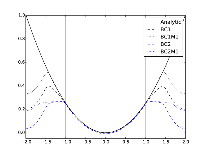
(a)

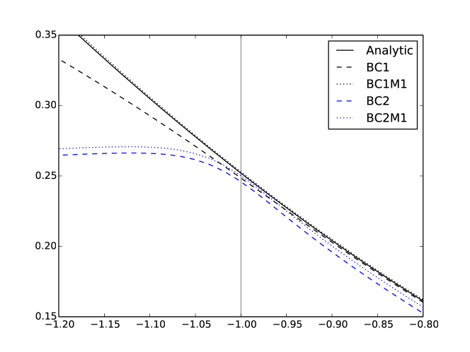
(b)

Figure 12: A plot of the solutions of Case 1 through $y=0$. The solutions with BC2M1 and BC2M2 are indistinguishable, so only BC2M1 is shown. (a) Shows the full slice, where the domain boundary is depicted as thin vertical lines at $x=\pm 1$. (b) A zoom-in that shows the solutions near the left boundary.

5 Conclusion

We have performed a matched asymptotic analysis of the DDM for the Poisson equation with Robin boundary conditions and for a steady reaction-diffusion equation with Neumann boundary conditions. Our analysis shows that for certain choices of the boundary condition approximations, the DDM is second-order accurate in the interface thickness $\epsilon$. However, for other choices the DDM is only first-order accurate. This is confirmed numerically and helps to explain why the choice of boundary-condition approximation is important for rapid global convergence and high accuracy. This helps to explain why the choice of boundary-condition approximation is important for rapid global convergence and high accuracy. In particular, the boundary condition BC1, which arises from representing the surface delta function as $|\nabla\phi|$, is seen to give rise to a second-order approximation for both the Neumann and Robin boundary conditions and thus is perhaps the most reliable choice. The boundary condition BC2, which arises from approximating the surface delta function as $\epsilon|\nabla\phi|^{2}$ yields a second-order accurate approximation for the Neumann problem, but only first-order accuracy for the Robin problem. In addition, BC2 requires very fine meshes to converge.

Our analysis also suggests correction terms that may be added to yield a more accurate diffuse-domain method. We have presented several techniques for obtaining second-order boundary conditions and performed numerical simulations that confirm the predicted accuracy, although the order of accuracy may deteriorate at the smallest values of $\epsilon$ possibly due to amplification errors associated with conditioning of the system or the influence of higher order terms in the asymptotic expansion. This is currently under study. Further, the correction terms do not improve the mesh requirements for convergence.

A common feature of the correction terms is that the interface thickness must be sufficiently small in order for the DDM to remain an elliptic equation. In addition, one choice of boundary condition involves the use of the surface Laplacian of the solution, which could in principle lead to faster asymptotic convergence since it directly cancels terms in the inner expansion of the asymptotic matching. However, the extension of this term outside the domain of interest can cause the loss of ellipticity of the DDM. As such, this is an intriguing but not a practical scheme. Nevertheless, as a proof of principle, we still considered the effect of this term, however, by using the surface Laplacian of the analytic solution in the DDM. We found that this choice gave the smallest errors in nearly all the cases considered. By incorporating different extensions of the boundary conditions in the exterior of the domain that automatically guarantee ellipticity, we aim to make this method practical. This is the subject of future investigations.

We plan to extend our analysis to the Dirichlet problem where the boundary condition approximations considered by Li et al. [42] seem only to yield first-order accuracy [22, 58]. Our asymptotic analysis thus has the potential to identify correction terms that can be used to generate second-order accurate diffuse-domain methods for the Dirichlet problem.

Acknowledgement. KYL acknowledges support from the Fulbright foundation for a Visiting Researcher Grant to fund a stay at the University of California, Irvine. KYL also acknowledges support from Statoil and GDF SUEZ, and the Research Council of Norway (193062/S60) for the research project Enabling low emission LNG systems. JL acknowledges support from the National Science Foundation, Division of Mathematical Sciences, and the National Institute of Health through grant P50GM76516 for a Center of Excellence in Systems Biology at the University of California, Irvine. The authors gratefully thank Bernhard Müller (NTNU) and Svend Tollak Munkejord (SINTEF Energy Research) for helpful discussions and for feedback on the manuscript. The authors also wish to thank the anonymous reviewers for comments that greatly improved the manuscript.

References

- [1] S. Aland, J. Lowengrub, and A. Voigt, Two-phase flow in complex geometries: A diffuse-domain approach., Computer Modeling in Engineering & Sciences, 57 (2010), pp. 77–106.
- [2] R. F. Almgren, Second-order phase field asymptotics for unequal conductivities, SIAM Journal on Applied Mathematics, 59 (1999), pp. 2086–2107.
- [3] J. Bedrossian, J. H. von Brecht, S. Zhu, E. Sifakis, and J. M. Teran, A second-order virtual node method for elliptic problems with interfaces and irregular domains, J. Comput. Phys., 229 (2010), pp. 6405-6426.
- [4] M.K. Bernauer, R. Herzog, Implementation of an X-FEM solver for the classical two-phase Stefan problem, J. Sci. Comput., 52 (2012), pp. 271-293.
- [5] A. Bueno-Orovio and V. M. Perez-Garcia, Spectral smoothed boundary methods: the role of external boundary conditions, Numer. Meth. Partial Diff. Eqns., 22 (2006), pp. 435–448.
- [6] A. Bueno-Orovio, V. M. Perez-Garcia, and F. H. Fenton, Spectral methods for partial differential equations in irregular domains: the spectral smoothed boundary method, SIAM Journal on Scientific Computing, 28 (2006), pp. 886–900.
- [7] A. Byfut, A. Schroeder, hp-adaptive extended finite element method, Int. J. Numer. Meth. Eng., 89 (2012), pp. 1293-1418.
- [8] G. Caginalp, P. C. Fife, Dynamics of Layered Interfaces Arising from Phase Boundaries, SIAM Journal on Applied Mathematics, 48 (1988), pp. 506–518.
- [9] M. Cisternino, L Weynans, A parallel second-order Cartesian method for elliptic interface problems, Comm. Comput. Phys., 12 (2012), pp. 1562-1587.
- [10] A. Coco and G. Russo, Finite-Difference Ghost-Point Multigrid Methods on Cartesian Grids for Elliptic Problems in Arbitrary Domains, J. Comput. Phys., 241 (2013), pp. 464-501.
- [11] A. Demlow and G. Dziuk, An adaptive finite element method for the Laplace-Beltrami operator on implicitly defined surfaces, SIAM J. Numer. Anal., 45 (2007), pp. 421-442.
- [12] J. Dolbow, I. Harari, An efficient finite element method for embedded interface problems, Int. J. Numer. Meth. Eng., 78 (2009), pp. 229-252.
- [13] R. Duddu, D.L. Chopp, P. Voorhees, B. Moran, Diffusional evolution of precipitates in elastic media using the extended finite element method and level set methods, J. Comput. Phys., 230 (2011), pp. 1249-1264.
- [14] G. Dziuk and C.M. Elliott, Eulerian finite element method for parabolic PDEs on implicit surfaces, Int. Free. Bound., 10 (2008), pp. 119-138.
- [15] G. Dziuk and C.M. Elliott, An Eulerian approach to transport and diffusion on evolving implicit surfaces, Comput. Visual. Sci., 13, (2010), pp. 17-28.
- [16] G. Dziuk and C.M. Elliott, A fully discrete evolving surface finite element method, SIAM J. Numer. Anal., 50, 5, (2012), pp. 2677-2694.
- [17] C.M. Elliott, B. Stinner, V. Styles, R. Welford, Numerical computation of advection and diffusion on evolving diffuse interfaces, IMA J. Num. Anal., 31, (2011), pp. 245-269.
- [18] C.M. Elliott and B. Stinner, Analysis of a diffuse interface approach to an advection diffusion equation on a moving surface, Math. Mod. Meth. Appl. Sci., (2009) in press.
- [19] R.P. Fedkiw, T. Aslam, B. Merriman, S. Osher, A non-oscillatory Eulerian approach to interfaces in multimaterial flows (the ghost fluid method, J. Comput. Phys., 152 (1999), pp. 457-492.
- [20] F. H. Fenton, E. M. Cherry, A. Karma, and W. J. Rappel, Modeling wave propagation in realistic heart geometries using the phase-field method, CHAOS, 15 (2005).
- [21] R. Folch, J. Casademunt, A. Hernandez-Machado, and L. Ramirez-Piscina, Phys. Rev. E, 60 (1999), pp. 1724.
- [22] S. Franz, R. Gärtner, H.-G. Roos, and A. Voigt, A Note on the Convergence Analysis of a Diffuse-Domain Approach, Computational Methods in Applied Mathematics, 12 (2012), pp. 153–167.
- [23] F.-P. Fries, T. Belytschko, The extended/generalized finite element method: An overview of the method and its applications, Int. J. Numer. Meth. Eng., 84 (2010), pp. 253-304.
- [24] F. Gibou, C. Min, and R. Fedkiw, High Resolution Sharp Computational Methods for Elliptic and Parabolic Problems in Complex Geometries, Journal of Scientific Computing, 54 (2013), pp. 369-413.
- [25] F. Gibou, R. Fedkiw, L.T. Cheng, and M. Kang, A second-order accurate symetric discretization of the Poisson equation on irregular domains, J. Comput. Phys., 176 (2002), pp. 205-227.
- [26] F. Gibou and R. Fedkiw, A fourth order accurate discretization for the Laplace and heat equations on arbitrary domains with applications to the Stefan problem, J. Comput. Phys., 202 (2005), pp. 577-601.
- [27] J. Glimm and D. Marchesin and O. McBryan, A numerical method for 2 phase flow with an unstable interface, J. Comput. Phys., 39 (1981), pp. 179-200.
- [28] R. Glowinski, T.W. Pan, and J. Periaux, A fictitious domain method for external incompressible viscous-flow modeled by Navier-Stokes equations, Comput. Meth. Appl. Mech. Engin., 112 (1994), pp. 133-148.
- [29] R. Glowinski and T.W. Pan and R.O. Wells and X.D. Zhou, Wavelet and finite element solutions for the Neumann problem using fictitious domains, J. Comput. Phys., 126 (1996), pp. 40-51.
- [30] J.B. Greer and A.L. Bertozzi and G. Sapiro, Fourth order partial differential equations on general geometries, J. Comput. Phys., 216 (2006), pp. 216-246.
- [31] S. Gross, and A. Reusken, An extended pressure finite element space for two-phase incompressible flows, J. Comput. Phys., 224 (2007), pp. 40-48.
- [32] X.M. He, T. Lin, Y.P. Lin, Immersed finite element methods for elliptic interface problems with non-homogeneous jump conditions, Int. J. Numer. Anal. Model., 8 (2011), pp. 284-301.
- [33] Á. Helgadóttir and F. Gibou, A Poisson–Boltzmann solver on irregular domains with Neumann or Robin boundary conditions on non-graded adaptive grid, J. Comput. Phys., 230 (2011), pp. 3830-3848.
- [34] J. L. Hellrung Jr., L. Wang, E. Sifakis, and J. M. Teran, A second order virtual node method for elliptic problems with interfaces and irregular domains in three dimensions, J. Comput. Phys., 231 (2012), pp. 2015-2048.
- [35] H. Ji and F.-S. Lien and E. Yee, An efficient second-order accurate cut-cell method for solving the variable coefficient Poisson equation with jump conditions on irregular domains, Int. J. Numer. Meth. Fluids, 52 (2006), pp. 723-748.
- [36] H. Johansen and P. Colella, A Cartesian grid embedded boundary method for Poisson’s equation on irregular domains, J. Comput. Phys., 147 (1998), pp. 60-85.
- [37] H. Johansen and P. Colella, Embedded boundary algorithms and software for partial differential equations, J. Phys., 125 (2008), pp. 012084.
- [38] A. Karma and W.-J. Rappel, Quantitative phase-field modeling of dendritic growth in two and three dimensions, Physical Review E, 57 (1998), pp. 4323–4349.
- [39] J. Kockelkoren, H. Levine, and W. J. Rappel, Computational approach for modeling intra- and extracellular dynamics, Phys. Rev., E 68 (2003), p. 037702.
- [40] R.J. Leveque and Z. Li, The immersed interface method for elliptic equations with discontinuous coefficients and singular sources, SIAM J. Numer. Anal., 31 (1994), pp. 1019-1044.
- [41] H. Levine and W. J. Rappel, Membrane-bound turing patterns, Physical Review E, 72 (2005).
- [42] X. Li, J. Lowengrub, A. Rätz, and A. Voigt, Solving pdes in complex geometries: A diffuse-domain approach, Communications in Mathematical Sciences, 7 (2009), pp. 81–107.
- [43] Z. Li and K. Ito, The immersed interface method: Numerical solutions of PDEs involving interfaces and irregular domains, SIAM Front. Appl. Math., 33 (2006).
- [44] Z. Li, P. Song, An adaptive mesh refinement strategy for immersed boundary/interface methods, Comm. Comput. Phys., 12 (2012), pp. 515-527.
- [45] R. Lohner and J.R. Cebral and F.F. Camelli and J.D. Baum and E.L. Mestreau and O.A. Soto, Adaptive embedded/immersed unstructured grid techniques, Arch. Comput. Meth. Eng., 14 (2007), pp. 279-301.
- [46] S.H. Lui, Spectral domain embedding for elliptic PDEs in complex domains, J. Comput. Appl. Math., 225 (2009), pp. 541-557.
- [47] P. Macklin and J. Lowengrub, Evolving interfaces via gradients of geometry-dependent interior Poisson problems: Application to tumor growth, J. Comput. Phys., 203 (2005), pp. 191-220.
- [48] P. Macklin and J. Lowengrub, A new ghost cell/level set method for moving boundary problems: Application to tumor growth, J. Sci. Comput., 35 (2008), pp. 266-299.
- [49] M. Oevermann, C. Scharfenberg, and R. Klein, A sharp interface finite volume method for elliptic equations on Cartesian grids, J. Comput. Phys., 228 (2009), pp. 5184-5206.
- [50] S. Osher and R. Fedkiw, Level set methods and dynamic implicit surfaces, Springer (2003).
- [51] S. Osher and J.A. Sethian, Fronts propagating with curvature-dependent speed: Algorithms based on Hamilton-Jacobi formulations, J. Comput. Phys., 79 (1988), pp. 12-49.
- [52] J. Papac, F. Gibou, and C. Ratsch, Efficient symmetric discretization for the Poisson, heat and Stefan-type problems with Robin boundary conditions, J. Comput. Phys., 229 (2010), pp. 875-889.
- [53] J. Papac, A. Helgadottir, C. Ratsch, and F. Gibou, A level set approach for diffusion and Stefan-type problems with Robin boundary conditions on quadtree/octree adaptive Cartesian grids, J. Comput. Phys., 233 (2013), pp. 241-261.
- [54] R. L. Pego, Front migration in the nonlinear Cahn-Hilliard equation, Proceedings of the Royal Society A, 422 (1988), pp. 261–278.
- [55] T. Preusser, M. Rumpf, S. Sauter, and L.O. Schwen, 3D composite finite elements for elliptic boundary value problems with discontinuous coefficients, SIAM J. Sci. Comput., 35 (2011), pp. 2115-2143.
- [56] I. Ramiere, P. Angot, and M. Belliard, A general fictitious domain method with immersed jumps and multilevel nested structured meshes, J. Comput. Phys., 225 (2007), pp. 1347-1387.
- [57] A. Rätz and A. Voigt, PDEs on surfaces—a diffuse interface approach, Commun. Math. Sci., 4 (2006), pp. 575-590.
- [58] M. G. Reuter, J. C. Hill, and R. J. Harrison, Solving pdes in irregular geometries with multiresolution methods i: Embedded Dirichlet boundary conditions, Computer Physics Communications, 183 (2012), pp. 1–7.
- [59] J.A. Sethian, Level set methods and fast marching methods, Cambridge University Press (1999), ISBN 0-521-64557-3.
- [60] J.A. Sethian and Y. Shan, Solving partial differential equations on irregular domains with moving interfaces, with applications to superconformal electrodeposition in semiconductor manufacturing, J. Comput. Phys., 227 (2008), pp. 6411-6447.
- [61] K. E. Teigen, X. Li, J. Lowengrub, F. Wang, and A. Voigt, A diffuse-interface approach for modeling transport, diffusion and adsorption/desorption of material quantities on a deformable interface, Communications in Mathematical Sciences, 7 (2009), pp. 1009–1037.
- [62] K.E. Teigen, P. Song, A. Voigt, and J. Lowengrub, A diffuse-interface method for two-phase flows with soluble surfactants, J. Comput. Phys., 230 (2011), pp. 375-393.
- [63] M. Theillard, L. F. Djodom, J.-L. Vié, and F. Gibou, A second-order sharp numerical method for solving the linear elasticity equations on irregular domains and adaptive grids – Application to shape optimization, J. Comput. Phys., 233 (2013), pp. 430-448.
- [64] E. Uzgoren, J. Sim, and W. Shyy, Marker-based, 3-D adaptive Cartesian grid method for multiphase flows around irregular, Comm. Comput. Phys., 5 (2009), pp. 1-41.
- [65] X.H. Wan and Z. Li, Some new finite difference methods for Helmholtz equations on irregular domains or with interfaces, Disc. Cont. Dyn. Sys. B, 17 (2012), pp. 1155-1175.
- [66] S. Wise, J. Kim, and J. Lowengrub, Solving the regularized, strongly anisotropic Cahn-Hilliard equation by an adaptive nonlinear multigrid method, Journal of Computational Physics, 226 (2007), pp. 414–446.
- [67] K. Xia, M. Zhan, and G. Wei, MIB method for elliptic equations with multimaterial interfaces, J. Comput. Phys., 230 (2011), pp. 4588-4615.
- [68] S. Zhao and G. Wei, Matched interface and boundary (MIB) for the implementation of boundary conditions in high-order central finite differences, Int. J. Numer. Meth. Eng., 77 (2009), pp. 1690-1730.
- [69] S. Zhao, High order matched interface and boundary methods for the Helmholtz equation in media with arbitrarily curved interfaces, J. Comput. Phys., 229 (2010), pp. 3155-3170.
- [70] X.L. Zhong, A new high-order immersed interface method for solving elliptic equations with imbedded interface of discontinuity, J. Comput. Phys., 225 (2007), pp. 1066-1099.
- [71] Y.C. Zhou, S. Zhao, M. Feig, and G.W. Wei, High order matched interface and boundary method for elliptic equations with discontinuous coefficients and singular sources, J. Comput. Phys., 213 (2006), pp. 1-30.
- [72] Y.C. Zhou, J. Liu, and D.L. Harry, A matched interface and boundary method for solving multiflow Navier-Stokes equations with applications to geodynamics, J. Comput. Phys., 231 (2012), pp. 223-242.
- [73] Y. Zhu, Y. Wang, J. Hellrung, A. Cantarero, E. Sifakis, and J. M. Teran, A second-order virtual node algorithm for nearly incompressible linear elasticity in irregular domains, J. Comput. Phys., 231 (2012), pp. 7092-7117.