On the low-field Hall coefficient of graphite

Abstract

We have measured the temperature and magnetic field dependence of the Hall coefficient ($R_{\rm H}$) in three, several micrometer long multigraphene samples of thickness between $\sim 9~{}$to $\sim 30$ nm in the temperature range 0.1 to 200 K and up to 0.2 T field. The temperature dependence of the longitudinal resistance of two of the samples indicates the contribution from embedded interfaces running parallel to the graphene layers. At low enough temperatures and fields $R_{\rm H}$ is positive in all samples, showing a crossover to negative values at high enough fields and/or temperatures in samples with interfaces contribution. The overall results are compatible with the reported superconducting behavior of embedded interfaces in the graphite structure and indicate that the negative low magnetic field Hall coefficient is not intrinsic of the ideal graphite structure.

I Introduction

The Hall effect is a fundamental transport property of metals and semiconductors. It can provide information on the carrier densities as well as on other interesting features of the electronic band structure. Surprisingly and in spite of considerable work in the past, the Hall coefficient ($R_{\rm H}$) of graphite, a highly anisotropic material composed by a stack of graphene layers with Bernal stacking order (ABA…), in particular the temperature and magnetic field dependence of $R_{\rm H}$ reported in literature is far from clear. For example, early data on the low-field Hall coefficient obtained in single-crystalline natural graphite (SCNG) samples showed that it is positive at fields below and negative above $\sim 0.5~{}$T at a temperature $T=77~{}$K Soule (1958), suggesting that holes are the majority carriers. This result appears to be at odd to several other studies on the graphite band structure obtained in highly oriented pyrolytic graphite (HOPG) samples Kelly (1981); Grüneis et al. (2008); Zhou et al. (2006a, b); Leem et al. (2008); Sugawara et al. (2007); Schneider et al. (2009); Orlita et al. (2008); Goncharuk et al. (2012) that suggest that electrons are the majority carriers, unless one argues in terms of different mobilities of the majority carriers, an interpretation that was used indeed in the past.

The difference between the reported Hall coefficient obtained in the SCNG and different HOPG samples was the subject of a short paper in 1970 where the authors concluded that the positive low-field Hall coefficient is observed for samples with long enough mean free path, i.e. less lattice defects, whereas the negative sign results from boundary scattering in HOPG samples due to the relatively small single crystalline grains Cooper et al. (1970). At high enough applied magnetic fields or high enough temperatures, this coefficient, however, turned negative Soule (1958); Cooper et al. (1970). A positive low-field Hall coefficient was already reported in 1953 for graphite samples with small crystal size (less annealing temperature); it decreased with temperature and changed sign at a sample dependent temperature Kinchin (1953). When the crystalline grain size in the samples was larger than $\sim 0.5~{}\mu$m, the Hall coefficient was always negative, at least at $T\geq 77~{}$K Kinchin (1953). Similar results were obtained in carbons and polycrystalline graphite samples with different crystal size in Ref. Mrozowski and Chaberski, 1956, where the authors recognized further that the Hall coefficient was highly dependent on the alignment of crystallites in the samples. Note that these two last reports Kinchin (1953); Mrozowski and Chaberski (1956) are in apparent contradiction to the relationship between crystal size and positive sign of $R_{\rm H}$ given in Ref. Cooper et al., 1970. It is therefore suggestive that one extra parameter related to the alignment of the crystalline grains in the samples could provide a hint to solve this contradiction.

In the studies of Ref Brandt et al., 1974 a positive Hall coefficient was reported at 4.2 K that became negative at $\mu_{0}H\geq 0.05$ T for different graphite samples. In that work Brandt et al. (1974) the positive low-field Hall coefficient was explained within the two-band model arguing that it is due to the higher mobility of the majority holes in comparison with the mobility of the majority electrons. However, to understand its behavior as a function of field and temperature, three types of carriers had to be introduced in the calculations Brandt et al. (1974). The low-field coefficient of different Kish graphite samples was reported in Ref. Oshima et al., 1982. For the “best” Kish sample, defined as the one with the largest resistivity ratio $\rho(300)/\rho(4.2)$, the Hall coefficient was positive at low fields and turned to negative at $\mu_{0}H\simeq 0.6~{}$T at 4.2 K, similarly to the results for some of the graphite samples reported in Ref. Brandt et al., 1974. The temperature dependence of the zero-field Hall coefficient for the “best” Kish specimen was interpreted Oshima et al. (1982) taking into account the trigonally warped Fermi surfaces in the standard Slonczewski-Weiss-McClure’s model Slonczewski and Weiss (1958); McClure (1958). Interestingly, the lesser the perfection of the Kish graphite samples the larger was the field where the Hall coefficient changed sign Oshima et al. (1982).

Recently published Hall measurements in micrometer small and thin graphite flakes, peeled off from HOPG samples, showed a positive and nearly field independent Hall coefficient at $T=0.1~{}$K up to 8 T applied fields Bunch et al. (2005). A positive Hall coefficient was also observed in similar graphite flakes at $77\leq T\leq 300~{}$K, which decreased with temperature, it was field independent to $\mu_{0}H\simeq 1$ T, decreasing at higher fields Vansweevelt et al. (2011). Interestingly, both results Bunch et al. (2005); Vansweevelt et al. (2011) are in rather good quantitative agreement with the result for the low-field Hall coefficient reported 56 years ago for the bulk SCNG Soule (1958), in clear contrast to reports in HOPG bulk samples Kelly (1981); Cooper et al. (1970); Kopelevich et al. (2003a); Kempa et al. (2006); Kopelevich et al. (2006a); Schneider et al. (2009).

Further studies on bulk HOPG samples showed the existence of an anomalous Hall effect and a negative Hall coefficient at low fields, interpreted as the result of a magnetic field induced magnetic excitonic state Kopelevich et al. (2006a). Also the quantum Hall effect (QHE) (with electrons as majority carriers) has been reported in some bulk HOPG samples at high enough fields Kopelevich et al. (2003a); Kempa et al. (2006). But the QHE in graphite as well as other interesting features of the Hall effect behavior like the hole-like contribution with zero mass Kopelevich and Esquinazi (2007) in bulk HOPG samples, appear to be strongly sample dependent Schneider et al. (2009). A short resume of the literature results can be seen in Table 1. Evidently, all these, apparently contradictory results indicate us that we need a re-evaluation of the sign, temperature and field behavior of the Hall coefficient. The whole reported studies show us that we do not know with certainty, which is the intrinsic value of the Hall coefficient in ideal graphite and which is the origin of all the observed differences between samples of different origins and microstructure.

$\bf{Ref.}$	$\bf{year}$	$\bf{sample}$	$\bf{T-range}$	$\bf{field-range}$	$\bf{R_{\rm H}}$	$\bf{comment}$
Kinchin,1953	1953	PCG	$\geq 4.2~{}$K	$<1~{}$T	positive	for small grains only3
Mrozowski and Chaberski,1956	1956	PCG	77 K/300 K	0.65 T	positive	for small grains only4
Soule,1958	1958	SCNG	$\leq 77~{}$K	$<$ 0.5 T	positive	negative at large fields and temperatures
Cooper et al.,1970	1970	HOPG/SCG	77 K	$<0.1~{}$T	positive	negative upon mean free path2
Brandt et al.,1974	1974	$({\dagger})$	4.2 K	$<$ 50 mT	positive	negative at higher fields
Oshima et al.,1982	1982	Kish graphite	4.2 K	$<$ 600 mT	positive	${R_{\rm H}(H)}$ changes sign5
Kopelevich et al.,2003a	2003	HOPG	0.1 K$\leq T\leq 20~{}$K	$\leq 9~{}$T	negative	quantum Hall effect (QHE)6
Bunch et al.,2005	2005	graphite flakes1	0.1 K	$<$ 8 T	positive
Kempa et al.,2006	2006	HOPG	2 K, 5 K	$\leq 9~{}$T	negative	quantum Hall effect (QHE)6
Kopelevich et al.,2006a	2006	HOPG	0.1 K$\leq T\leq 100~{}$K	$\leq 0.5~{}$T	negative	Anomalous Hall effect
Schneider et al.,2009	2010	NG/HOPG	10 mK	$<$ 10 T	negative	($\ast$)
Vansweevelt et al.,2011	2011	graphite flakes1	$77\leq T\leq 300$ K	$<$ 1 T	positive

Table 1: Selected publications that report on the Hall coefficient $R_{\rm H}$ of different graphite samples at different fields and temperatures. NG: natural graphite, SCNG: single crystal natural graphite, PCG: polycrystalline graphite. ¹Peeled off from HOPG. ${}^{2}{R_{\rm H}}>0$ for long mean free path, ${R_{\rm H}}<0$ for short mean free path or at higher fields. ³Negative for grain size $>0.5\mu$m. Crossover from positive to negative at a sample dependent temperature. ⁴Positive $R^{0}_{\rm H}$ for small grains, negative for grain size $>0.5\mu$m, and strong orientation dependence of $R^{0}_{\rm H}$. ⁵ Turns negative at large field for samples with imperfect structure.⁶With electrons as majority carriers. ($\ast$): No Hall data shown at low fields. (${\dagger}$): The samples were obtained by crystallization from a solution of carbon in iron and then purified at 2000^∘C in a flux of chlorine. The platelets had a thickness of $\sim 100~{}\mu$m $\lesssim d\lesssim 9~{}$mm.

In this work, we argue that one main reason for the observed differences of the Hall coefficient between samples is related to the existence of two dimensional (2D) interfaces Inagaki (2000); Barzola-Quiquia et al. (2008); García et al. (2012). Moreover, in some of them Josephson coupled superconducting regions exist, oriented parallel to the graphene layers of the graphite matrix Ballestar et al. (2013); Scheike et al. (2013); Esquinazi et al. (2014). The interfaces in graphite, whose contribution to the Hall effect we discuss in this work, are grain boundaries between crystalline domains with slightly different orientations. Those crystalline domains and the two-dimensional borders between them, can be recognized by transmission electron microscopy when the electron beam is applied parallel to the graphene planes of graphite, see e.g. Fig. 1 in Ref. Esquinazi et al., 2014, Fig. 1 in Ref. Barzola-Quiquia et al., 2008 or Figs. 2.2 and 2.9 in Ref. Inagaki, 2000. The interfaces can be located at the borders of slightly twisted crystalline Bernal stacking order regions (ABA…) or between regions with Bernal and rhombohedral staking order (ABCAB…) regions. They can be recognized usually by a certain gray colour in the TEM pictures Esquinazi et al. (2014); Barzola-Quiquia et al. (2008). From TEM pictures we obtain that the distance between those interfaces can be between $\sim 30~{}$nm and several hundreds of nm upon sample Barzola-Quiquia et al. (2008); Scheike et al. (2013). Therefore, the thinner the graphite sample the lower the probability to have interfaces and to measure their contribution to any transport property.

The twist angle $\theta_{\rm twist}$, i.e., a rotation with respect to the $c-$axis between single crystalline domains of Bernal graphite, may vary from $\sim 1^{\circ}$ to $<60^{\circ}$ Warner et al. (2009) while the tilting angle of the grains with respect to the $c$-axis $\theta_{\rm c}\lesssim 0.4^{\circ}$ for the best oriented pyrolytic graphite samples. As emphasized in Ref. Esquinazi et al., 2014, in case the twist angle is small enough, the grain boundary can be represented by a system of screw dislocations or a system of edge dislocations if the misfit is in the c-direction with an angle $\theta_{\rm c}\neq 0$. A system of dislocations at the two-dimensional interfaces or topological line defects can have a large influence in the dispersion relation of the carriers Feng et al. (2012); San-Jose and Prada (2013) and trigger localized high-temperature superconductivity Volovik (2014).

There have been several theoretical studies predicting high temperature superconductivity at the rhombohedral (ABC) graphite surface Kopnin et al. (2011, 2013); Volovik (2013) or at interfaces between rhombohedral and Bernal (ABA) graphite Muñoz et al. (2013); Kopnin and Heikkilä . We note that rhombohedral graphite regions were also recognized embedded in bulk HOPG samples Lin et al. (2012); Hattendorf et al. (2013). Theoretical studies indicate an unusual dependence of the superconductivity at the surface of rhombohedral graphite or at the interfaces between rhombohedral and Bernal (ABA) graphite in multilayer graphene on doping Muñoz et al. (2013). Furthermore, calculations indicate that high-temperature surface superconductivity survives throughout the bulk due to the proximity effect between ABC/ABA interfaces where the order parameter is enhanced Muñoz et al. (2013). Following experimental results that indicate the existence of granular superconductivity at certain interfaces in bulk HOPG samples of high grade Ballestar et al. (2013); Scheike et al. (2013); Ballestar et al. (2014), it is then appealing to take the contribution of the interfaces in the behavior of the Hall effect into account. Doing this we are able to interpret several results from literature as well as the Hall coefficient obtained from three, micrometer small graphite flakes described below. The characteristics of the embedded interfaces, as for example their size or area Ballestar et al. (2014) or the twist angle between the two Bernal graphite blocks Esquinazi et al. (2014) can have a direct influence on the temperature and magnetic field dependence of the Hall coefficient of a graphite sample with interfaces. Furthermore, the alignment dependence reported earlier Mrozowski and Chaberski (1956) can be understood arguing that the interfaces are created or get larger in area the higher the alignment of the grains. From the presented work we can conclude that the intrinsic low magnetic field Hall coefficient of ideal graphite is positive, i.e. hole like. It can change to negative in samples with embedded interfaces at fields and temperatures high enough to influence their contribution. On the other hand one expects that if the interfaces are not superconducting in a given sample, they will provide an electron-like contribution to the Hall resistance, which may or may not overwhelm the intrinsic Hall signal of graphite.

II Experimental details

The graphite flakes we have measured were obtained by a rubbing method on Si-SiN substrates using a bulk HOPG sample of ZYA grade from Advanced Ceramics Co. These samples show, in general, well defined quasi-two dimensional interfaces between Bernal graphite structures with slightly different orientation around the $c-$axis. Their distance in the $c-$axis direction is sample dependent and in general $<500$ nm and of several micrometer length in the ($a,b$) plane Inagaki (2000); Barzola-Quiquia et al. (2008); Scheike et al. (2013). The Pt/Au contacts for longitudinal and transverse Hall resistance measurements were prepared using electron beam lithography. The samples with their substrates were fixed on a chip carrier. Further details on the preparation can be read in Barzola-Quiquia et al. (2008). We have measured three samples labeled S1, S2 and S3 with similar lateral dimensions but with thickness: $~{}9\pm 1~{}$nm (S2), $~{}20\pm 4~{}$nm (S1) and $~{}30\pm 3~{}$nm (S3). An example of one of the samples is shown in Fig. 1.

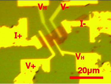
Figure 1: Optical microscope picture of sample S1 with the two current and four voltage gold contacts after lithography development and evaporation of Pt/Au contacts.

The transport measurements were carried out using the usual four-contacts methods in a conventional He⁴ cryostat and two of the samples (S1,S2) were also measured in a dilution refrigerator. Static magnetic fields were provided by superconducting solenoids applied always parallel to the $c-$axis. The longitudinal and transverse resistances were measured using a low-frequency AC bridge LR700 (Linear Research). After checking the ohmic response in both voltage electrodes of the samples, all the measurements were done with a fixed current of $1~{}\mu$A, which means a dissipation $\mathrm{d}Q/\mathrm{d}t<0.1~{}$nW to avoid self heating effects. In this work we focus on the Hall coefficient obtained at fields $\mu_{0}H\lesssim 0.2~{}$T.

III Results and discussion

III.1 Temperature dependence of the longitudinal resistance

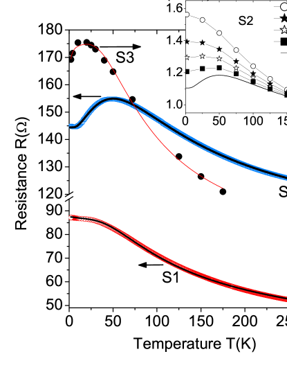
Figure 2: Resistance vs. temperature for the three multigraphene samples discussed in this work. The measurements were made without any applied field. The continuous lines were calculated following the parallel-resistor model from Ref. García et al., 2012, see text. The inset shows the normalized resistance vs. temperature at different fields applied normal to the interfaces for sample S2.

Figure 2 shows the electrical longitudinal resistance of the three samples vs. temperature at zero applied field. Following the results and the discussion exposed in Ref. García et al., 2012, we assume that ideal graphite is a narrow-gap semiconductor. The observed semiconducting-like temperature dependence in the longitudinal resistance has been also reported recently for thin graphite flakes Vansweevelt et al. (2011). We assume that any deviation from a semiconducting-like dependence in the longitudinal resistance is due to extrinsic contributions. The observed behavior in our samples is similar to that already published Barzola-Quiquia et al. (2008) and it can be understood taking into account the contributions of the semiconducting graphene layers in parallel to that from the embedded interfaces and of the sample surfaces (open and with the substrate) García et al. (2012). The interfaces’ contribution is responsible for the maximum in the resistance observed at $\sim 50~{}$K and $\sim 20~{}$K for samples S2 and S3, respectively. We speculate that the sample surfaces are responsible for the saturation of the resistance at low temperatures, as in S1 for example. The embedded interface contribution appears to be weaker in sample S1 than in the other two samples, therefore we expect for this sample a Hall coefficient with less extrinsic contributions than for the other two.

With a simple parallel-resistor model one can understand quantitatively the measured temperature dependence using different weights between the parallel contributions following the relation García et al. (2012):

$$R(T)=(R_{i}^{-1}(T)+R_{b}^{-1}(T))^{-1}\,,$$ (1)

see Fig. 2. The bulk, intrinsic contribution of graphite is semiconducting-like

$$R^{-1}_{b}(T)\simeq(A\exp(E_{g}/2k_{B}T))^{-1}+R_{d}^{-1}\,,$$ (2)

and the one from the interfaces and surfaces can be simulated following

$$R_{i}(T)=R_{0}+R_{1}T+R_{2}\exp(-E_{a}/k_{B}T)\,,$$ (3)

whereas the parameters $A,R_{j}(j=0,1,d)$ are free. The constant term $R_{d}$ prevents an infinite resistance from the bulk contribution, which is physically related to defects or (a) surface band(s). $E_{g},E_{a}$ denote the semiconducting gap and an activation energy; their values depend on sample within the range $250~{}$K $\lesssim E_{g}\lesssim 500~{}$K and $10~{}$K $\lesssim E_{a}\lesssim 50~{}$K García et al. (2012). The linear in temperature term ($R_{1}T$) could be negative or positive and it is taken as a guess for the contribution of the surfaces and/or metallic-like interfaces. The thermally activated function can be interpreted as the contribution of non-percolative, granular superconducting regions inside the internal interfaces embedded in the graphite matrix García et al. (2012), similar to that observed in granular Al in a Ge matrix Shapira and Deutscher (1983), for example. Transport Ballestar et al. (2013) as well as magnetization Scheike et al. (2013) measurements support the existence of granular superconductivity and Josephson coupling between superconducting regions at these interfaces.

At fields of the order of 0.1 T applied perpendicular to the interfaces, the metallic-like behavior (at $T<50~{}$K) starts to vanish, see the results of sample S2 in the inset of Fig. 2, as example. This behavior is assigned to the field-driven superconductor- (or metal-) insulator transition Kempa et al. (2000); Kopelevich et al. (2003a); Tokumoto et al. (2004); Du et al. (2005). Because this behaviour is absent in thin enough graphite flakes Barzola-Quiquia et al. (2008); García et al. (2012) or in thicker graphite samples without well defined interfaces, the field-driven transition is not intrinsic of ideal graphite and should not be interpreted in terms of band models for graphite with Bernal stacking order Tokumoto et al. (2004); Du et al. (2005). If this field-driven transition is compatible with the existence of Josephson coupled superconducting regions at the interfaces Ballestar et al. (2013); García et al. (2012); Scheike et al. (2013), we therefore expect that the Hall coefficient should be influenced at similar applied fields, as we show below.

III.2 Temperature dependence of the low-field Hall coefficient

The low-field Hall coefficient is defined as the $R^{0}_{\rm H}=d\lim_{H\rightarrow 0}r_{\rm H}/\mu_{0}H$, where $r_{\rm H}$ is the Hall resistance and $d$ the measured thickness of the sample. Figure 3 shows the temperature dependence of $R^{0}_{\rm H}(T)$ for the three samples measured in this work. We note that it changes sign at $\sim 45~{}$K and $\sim 70~{}$K for samples S3 and S2. For sample S1, $R^{0}_{\rm H}(T)$ remains positive in the whole measured temperature range. The observed behavior of $R^{0}_{\rm H}$ for sample S1 as well as its absolute value are similar to the recently reported ones for a mesoscopic graphite flake of similar thickness Vansweevelt et al. (2011). Due to the large dispersion of Hall coefficients and their variation with temperature found in literature (see Table I in Sec. I), this agreement is remarkable and support early results on a positive $R^{0}_{\rm H}$ at low enough fields and temperatures for graphite Soule (1958); Cooper et al. (1970).

All the three samples show positive, saturating $R^{0}_{H}(T\lesssim 25$ K), see Fig. 3. The origin of the differences between the low-field Hall coefficients at low temperatures is not known with certainty. A quantitative comparison of the absolute values of the Hall coefficient between different graphite samples is not straightforward because different samples have different interface contributions. The density of these interfaces as well as the number of those that have superconducting properties depend on the sample and it is not simply proportional to the thickness of the sample. Also different absolute values could arise from differences between the properties of holes and electron carriers, see Eq. (4), whose densities and mobilities can be influenced by defects and impurity atoms. Therefore, differences in the absolute values of the Hall coefficient between the samples should be taken with some care.

III.2.1 The intrinsic Hall coefficient

Taking into account the $T-$dependence of the longitudinal resistance, the results of Ref. García et al., 2012 and the fact that $R^{0}_{\rm H}(T)$ is positive, at least a two-band model Kelly (1981) is necessary to interpret the data. According to this model, the Hall coefficient is given by:

$$R^{0}_{H}=\frac{\mu_{p}^{2}p-\mu_{n}^{2}n}{e(\mu_{p}p+\mu_{n}n)^{2}}\,,$$ (4)

where $\mu_{p,n}$ are the mobilities for holes with density $p$ and electrons with density $n$, respectively; $e$ is the positive defined electronic charge. Since $R^{0}_{H}>0$, then $\mu_{p}^{2}p>\mu_{n}^{2}n$.

Taking into account the expected band structure of graphite and for practical purposes, we can assume either: (1) both mobilities are equal and that the carrier densities are related through $p=n+\delta>n$ with $\delta\ll p,n$, or (2) $\mu_{p}=\mu_{n}+\delta>\mu_{n}$, $p=n$ and $\delta\ll\mu_{p},\mu_{n}$. In both cases $p+n\simeq 2p$ and Eq. (4) can be approximated by either:

$$R^{0}_{\rm H} \simeq \frac{\delta}{4ep^{2}}~{}\textrm{with~{}}\delta=p-n$$ (5)

or

$$R^{0}_{\rm H} \simeq \frac{\delta}{2ep\mu_{p}}~{}\textrm{with~{}}\delta=\mu_{p}-\mu_{n}\,.$$ (6)

Obviously, the use of the one-band model equation, i.e. $R^{0}_{H}=1/pe$, provides incorrect values for the carrier concentration. For example, in Ref. Vansweevelt et al., 2011 the authors obtained $p(77~{}$K) $\simeq 7.7\times 10^{19}~{}$cm^-3 or $p_{2D}(77~{}$K)$\simeq 2.5\times 10^{12}~{}$cm^-2 per graphene layer. Using the same one-band model we would obtain for sample S1, $p_{2D}\simeq 8\times 10^{12}~{}$cm^-2, a value four orders of magnitude larger than the one obtained for similar samples using a model independent constriction method Dusari et al. (2011). Moreover, for such large $p$ values the use of Eq. (5) would give $\delta\gtrsim p$ using the measured $R^{0}_{H}$. However, if we take the carrier concentration $p_{2D}(75~{}$K$)\simeq 5\times 10^{8}$cm^-2 (or $p_{3D}\simeq 1.6\times 10^{16}$cm^-3) from Ref. Dusari et al., 2011, using Eq. (5) we obtain $\delta/p=2.5\times 10^{-4}$, indicating a very small difference between electron and hole carrier densities. Or using Eq. (6) we obtain $\delta/\mu_{p}\simeq 1\times 10^{-4}$, indicating a very small difference between the electron and Hall mobilities.

For sample S1, $R^{0}_{\rm H}(T)$ can be understood as the parallel contributions Petritz (1958) from the graphene layers with $p(T),n(T)\propto\exp(-E_{g}/2k_{\rm B}T)$ and a roughly temperature independent term (from the surfaces or some internal interfaces) that prevents the divergence of $R^{0}_{\rm H}(T\rightarrow 0)$. Using the same energy gap that fits the longitudinal resistance, we can fit $R^{0}_{\rm H}(T)$ in the whole $T-$range, see Fig. 3.

III.2.2 Interface contribution to the Hall coefficient

The results for $R^{0}_{H}(T)$ of sample S1 and those from ref. Vansweevelt et al., 2011 indicate us that the sign change above certain temperature in samples S3 and S2 should be related with the contribution of interfaces. Real graphite samples with interfaces are rather complex systems in the sense that the distribution of input electrical currents inside the sample is not homogeneous. Without knowing this distribution and the intrinsic conductivities of the different contributions, quantitative models are only under certain assumptions applicable. To estimate the interface contribution we use the model proposed in Ref. Petritz, 1958 for a bilayer, where the Hall coefficient of the surface (in our case the interfaces $R^{i}_{H}(T)$) and bulk ($R^{b}_{H}(T))$ contribute in parallel. The total measured Hall coefficient is given by

$$R_{\rm H}=\frac{d(R^{b}_{\rm H}\sigma^{2}_{b}d_{b}+R^{i}_{\rm H}\sigma^{2}_{i}d_{i})}{(\sigma_{b}d_{b}+\sigma_{i}d_{i})^{2}}\,,$$ (7)

where $\sigma_{b,i}$ are the conductivities of the bulk and interface contributions and $d_{b,i}$ the respective effective thicknesses, i.e. the total thickness of the sample is $d=d_{b}+d_{i}$. Taking into account the interface density in our HOPG samples obtained from transmission electron microscopy Barzola-Quiquia et al. (2008), we estimate $d_{i}/d_{b}\lesssim 10^{-2}$. In this case Eq. (7) can be written as:

$$R_{\rm H} \sim \frac{R^{b}_{H}+R^{i}_{H}r_{2}}{r_{1}}\,,$$ (8)

$$r_{1} = (1+r^{\prime}_{1})^{2},r^{\prime}_{1}=\frac{\sigma_{i}d_{i}}{\sigma_{b}d_{b}}\,,$$ (9)

$$r_{2} = \frac{\sigma_{i}^{2}d_{i}}{\sigma_{b}^{2}d_{b}}=r^{\prime 2}_{1}\frac{d_{b}}{d_{i}}\,.$$ (10)

The effective parallel contribution of the interfaces can be estimated from

$$R^{i}_{H}\sim\frac{R_{\rm H}r_{1}-R^{b}_{H}}{r_{2}}\,.$$ (11)

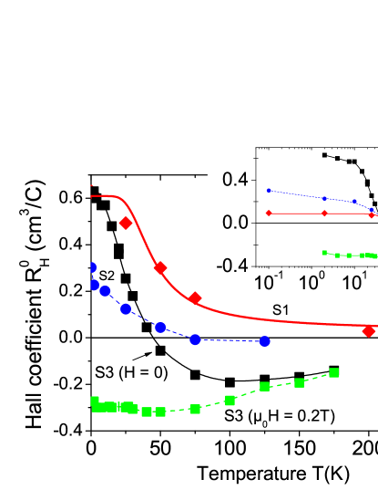
Figure 3: Temperature dependence of the low-field Hall coefficient for the three studied samples. For sample S3 (black squares) we show also the Hall coefficient (green squares) obtained at a field $\mu_{0}H=0.2~{}$T applied normal to the interfaces. The data from sample S1 in the main panel of the figure were multiplied by a constant factor of 6.7. The inset shows the same data but in a logarithmic temperature scale. The line through the S1 data points follows the function $R^{0}_{\rm H}=(11^{-1}+(4\times 10^{-3}\exp(300/(2T)))^{-1})^{-1}$. All other lines are only a guide to the eye.

In clear contrast to sample S1, the $R^{0}_{\rm H}(T)$ of sample S3 turns to negative at $T>45~{}$K. We propose that the origin for the sign change of $R^{0}_{\rm H}(T)$ increasing $T$ is due to the extra contribution of the interfaces when the superconducting properties of the interfaces vanish. At low enough temperatures the interfaces with the superconducting regions Ballestar et al. (2013) do not contribute substantially to the total low-field Hall effect. Because we are dealing here with the zero- or low-field Hall coefficient, vortices or fluxons (and their movement) are not expected to influence the Hall signal.

For sample S3 and using Eq. (11) we assume that $R^{i}_{\rm H}(T\ll 50~{}$K$)\simeq 0$ implying $R^{0}_{\rm H}r_{1}\ggg R^{b}_{\rm H}$. If we assume further that the total low-field Hall coefficient for this sample and at low temperatures is mainly given by the bulk contribution, we can roughly estimate the expected contribution from the interfaces. Using the functions that fit the temperature dependence of the measured resistance, see Fig. 2, the related conductivities can be estimated from $\sigma^{-1}_{i}\sim g_{i}(140-0.045T+10\exp(-4/T))$ and similarly for the bulk contribution $\sigma^{-1}_{b}\sim g_{b}(80\exp(350/2T))$, where the constant prefactors $g_{b,i}\sim w_{b,i}\times d_{b,i}/\ell_{b,i}$ (width $\times$ thickness $/$ length) are due to the different effective geometry of the two contributions. Note that neither the samples have perfectly rectangular shape nor the internal interfaces are expected to follow perfectly the measured external sample geometry. We estimate the Hall coefficient due to the bulk contribution as $R^{b}_{\rm H}(T)\sim(20^{-1}+(0.1\exp(350/2T))^{-1})^{-1}$ assuming that the saturation of $R^{0}_{\rm H}$ we measured for this sample, see Fig. 4, can be included in $R^{b}_{\rm H}$. Assuming $d_{b}/d_{i}=50$, we estimate the interface contribution to the Hall coefficient using Eq. (11) for three values of the factor $w_{b}\ell_{i}/w_{i}\ell_{b}$ that enters in $r^{\prime}_{1}$. The three curves can be seen in Fig. 4. The uncertainty in the geometrical factors and in the bulk Hall contribution do not allow a better quantitative estimate of the interface contribution. Nevertheless, qualitatively the obtained results for $R^{i}_{\rm H}(T)$ appear reasonable.

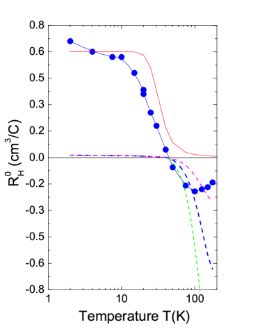
Figure 4: Temperature dependence of the low-field Hall coefficient for the S3 sample. The red line follows the equation $R^{b}_{\rm H}=0.03(20^{-1}+(0.1\exp(350/(2T)))^{-1})^{-1}$ used as the bulk contribution to the Hall coefficient for that sample. The dashed lines represent the contribution from the interfaces $R^{i}_{\rm H}(T)$ calculated from Eq. (11) assuming different geometrical ratios $w_{b}\ell_{i}/w_{i}\ell_{b}=200,300,500$, from bottom to top lines, respectively.

III.3 Magnetic field dependence of the Hall coefficient

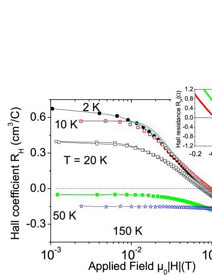
Figure 5: Hall coefficient as a function of the absolute value of the applied field at several temperatures for sample S3. The inset shows the field dependence of the Hall resistance at two temperatures.

We emphasize that for graphite samples with no measurable evidence for the interface contribution, in the electrical resistivity for example, the Hall coefficient does not depend on the field, at least up to 1 T applied normal to the graphene planes Bunch et al. (2005); Vansweevelt et al. (2011). Therefore, a direct way to test our assumption that the Hall coefficient and its negative value is not intrinsic – but due to the extra contribution from the embedded interfaces with superconducting regions – can be independently done measuring it at finite magnetic fields applied normal to the interfaces. In this case we expect that a magnetic field will have the same influence on the interface contribution as the temperature. In other words, a large enough magnetic field will destroy the coupling between the superconducting regions, or the superconductivity itself at the interfaces and an extra, electron-like contribution should be measurable, in principle in the whole temperature range. Note that mostly electron-like carriers are expected to be at the interfaces with a density of the order of $\lesssim 10^{12}~{}$cm^-2. This is inferred from Shubnikov-de Haas (SdH) oscillations in the magnetoresistance obtained in samples with and without (or with less number of) interfaces, see, e.g., Ref. Barzola-Quiquia et al., 2008 (compare there samples L5 and L7) or Ref. Ohashi et al., 2001 where a clear decrease in the amplitude of the SdH oscillations decreasing the thickness of the samples has been reported earlier. The reason why mostly electron-like carriers appear to be at the interfaces is related to the nature of the interfaces themselves, a subject that is being discussed nowadays, see Ref. Esquinazi et al., 2014 and Refs. therein. For example, in addition to the twist angle between the graphite Bernal blocks forming an interface, one has extra doping through hydrogen or carbon vacancies that influence the carrier density and the superconducting regions at the interfaces. For interfaces without superconducting regions we expect an electron-like contribution to the Hall coefficient with a weaker field and temperature dependence.

How large should be the magnetic field to affect the coupling between the superconducting regions or the superconductivity of the regions itself? An estimate of this field can be directly obtained from the longitudinal resistance and the metal-insulator transition (MIT) observed in several high grade graphite samples, as, e.g., in sample S2, see inset in Fig. 2, or several other samples reported in literature Kopelevich et al. (2003b, a); Tokumoto et al. (2004); Du et al. (2005). From all the results for the longitudinal resistance we expect that a field of the order of 0.1 T should be sufficient to influence substantially the Hall coefficient contribution of the interfaces. Note that the MIT of graphite is absent for samples without or with negligible amount of interfaces Barzola-Quiquia et al. (2008); García et al. (2012); Vansweevelt et al. (2011); Bunch et al. (2005). Figure 3 shows the Hall coefficient of sample S3 at a field of 0.2 T. It remains nearly temperature independent below 100 K and matches the results obtained at low-fields at high enough temperatures.

Figure 5 shows the field dependence of $R_{\rm H}$ at various constant temperatures where we recognize a transition from positive to negative values at fields similar to those necessary to trigger the metal-insulator transition observed in the longitudinal resistance. The results shown in this figure clearly indicate that a magnetic field has the same influence on the Hall coefficient as temperature. Note also that a field of the order of 0.1 T is enough to change the sign of the Hall coefficient in the sample with clear contribution of the interfaces.

Apart from the interface effects, one may expect a decrease of the (positive) Hall coefficient with field, at large enough fields when the cyclotron energy $\hbar\omega_{c}$ is of the order of the energy gap $E_{g}$ ($\omega_{c}=e\mu_{0}H/m^{\star}$ and $m^{\star}$ the effective electron mass, according to Ref. Cohen and Falicov, 1961. Because in graphite $E_{g}\lesssim 50~{}$meV this effect may start be observable at $\mu_{0}H>1~{}$T. On the other hand, data obtained from very thin graphite samples clearly show that the Hall coefficient is field independent up to 10 T at $T=0.1~{}$K Bunch et al. (2005), or up to 1 T at $T\geqslant 77~{}$K Vansweevelt et al. (2011). Therefore, we can clearly argue that the observed field dependence in our sample, see Fig. 5, is not intrinsic of the graphite structure but has an extrinsic origin, similar to that reported earlier Soule (1958); Cooper et al. (1970).

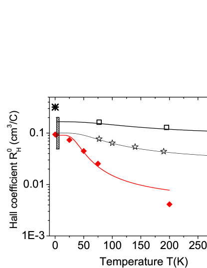
Figure 6: Low-field Hall coefficient as a function of temperature for sample S1 from this work (red lozenge); the line through the points follows the equation $(11+(0.004\exp(300/2T))^{-1})^{-1}$. The other points are taken from different graphite samples reported in literature. $(\star)$: Taken from Ref. Vansweevelt et al., 2011 for a graphite thin flake; the line through the points follows the equation $(10+(0.03\exp(350/2T))^{-1})^{-1}$. $(\square)$: Taken from Ref. Kinchin, 1953; the line through the points follows the equation $(6+(0.15\exp(400/2T))^{-1})^{-1}$. The vertical dashed region at low temperatures with $0.05\leq R^{0}_{H}\leq 0.2$ cm³/C is from Ref. Brandt et al., 1974. $(\ast)$: Hall coefficient at 100 mK obtained for a 5 nm thick graphite sample from Ref. Bunch et al., 2005.

IV Comparison with literature and conclusion

In a recent theoretical workPal and Maslov (2013), the magnetoresistance and Hall resistivity for graphite has been calculated using the usual 3D band structure described by the Slonczewski-Weiss-McClure model and taking into account only some of its six free parameters Brandt et al. (1988). The obtained results indicate that at relatively weak applied magnetic fields $<1~{}$T, the magnetoresistance increases linearly with field due to the presence of extremely light, Dirac-like carriers. Interestingly, in the same field range the authors found that the Hall coefficient should be positive and proportional to $\ln|B|$. We note that a linear field magnetoresistance was indeed reported in this field range and at low $T$ in a large amount of graphite samples, especially for relatively thick graphite samples, see for example the magnetoresistance curves for sample L7 (75 nm thick) in Ref. Barzola-Quiquia et al., 2008. Due to the observed positive Hall effect at low fields $<0.2~{}$T and at low temperatures, it is of interest to check whether such a linear field dependence is observed in the samples described in this work. Figure 7 shows the magnetoresistance vs. applied field below 0.2 T for the three samples and at low temperatures. Interestingly, none of the samples show a clear linear field dependence. The sample S1, which has the smallest contribution from interfaces (see Fig. 2) follows approximately a $H^{1.5}$ dependence. The other two samples, S2 and S3 tends to follow a quadratic dependence at low enough fields changing to a $\sim H^{1.3}$ dependence at higher fields, in agreement with similar measurements but in bulk HOPG samples Kopelevich et al. (2006b). Note that the absolute value of the magnetoresistance at a given field for our mesoscopic samples is much smaller than in bulk samples. As an example, we show in Fig. 7 the results for a bulk HOPG sample of grade A. In the depicted field region the magnetoresistance follows $\sim H^{1.25}$ but it is 200 times larger than in the other mesoscopic samples. This difference might be related to the size dependence of the magnetoresistance when the mean free path is of the order of the sample size González et al. (2007); Dusari et al. (2011). The field dependence in this low field region, however, does not seem to be affected.

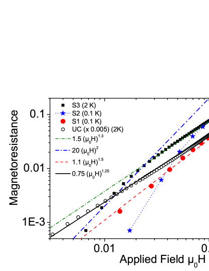
Figure 7: Low-field magnetoresistance defined as $R(B)-R(0)/R(0)$ vs. applied field in a double logarithmic scale, for the three samples studied in this work. The data of samples S1 and S2 were taken at 0.1 K and of sample S3 at 2 K. In the same panel we show the data for a bulk HOPG sample of grade A ($\circ$) obtained at 2 K.

We note that in the same field range we did not see an increasing Hall coefficient with field in any of the samples studied here. Also, for the graphite samples reported in Ref. Vansweevelt et al., 2011 at $T\geq 77~{}$K the Hall coefficient is constant below 1 T and decreases above. In the case of the $\simeq 1\times 1~{}\mu$m² sample reported in Ref. Bunch et al., 2005 we note that the magnetoresistance is negligible to 10 T applied field and $T=0.1~{}$K, a result related to the ballistic behavior of the carriers due to their large mean free path Dusari et al. (2011), and the Hall coefficient does not depend on field.

A comparison of the Hall coefficient and in general of the Hall data from literature is not straightforward because the sample quality as well as the existence of interfaces (of any kind) was not provided in any of the publications and remains, in general, unknown. Nevertheless, we can speculate the following trends and provide a possible answer to the works listed in Tab. 1. In Refs. Kinchin, 1953; Mrozowski and Chaberski, 1956, a positive Hall effect was observed for small grains only. Upon preparation conditions, smaller grains should have less interfaces, see section I, and therefore less contribution from them. Note that the reported dependence of $R_{H}$ on the alignment of the crystallites can be directly related to the larger probability to have well-defined and larger interfaces the larger the alignment of the crystallites is. Note that effective critical temperature depends on the size or area of the interfaces according to recently published experimental resultsBallestar et al. (2014). The crossover to a negative Hall coefficient at large enough fields and temperatures observed in Refs. Soule, 1958; Brandt et al., 1974; Oshima et al., 1982; Schneider et al., 2009 can be understood in a similar way as shown in sections III.2.2 and III.3. In Ref. Cooper et al., 1970 the Hall coefficient was reported to be positive for samples with long mean free path of the carriers and negative for samples with smaller mean free path or high fields. The crossover to a negative $R_{H}$ can be understood in the same way if some of the interfaces get normal conducting with field. Now, the reported mean free path dependence of $R_{H}$ cannot be simply interpreted in terms of interfaces contribution without knowing the internal structure of the samples and whether there is or not a crossover to negative $R_{H}$ at higher fields and temperatures. If we assume that the carriers in the graphene layers of graphite have much larger mobilityDusari et al. (2011) than those carriers at the interfaces in the normal state, we may speculate that samples with smaller mean free path have larger density of interfaces and therefore a negative $R_{H}$ should be measured.

The negative QHE measured in the HOPG samples in Refs. Kopelevich et al., 2003a; Kempa et al., 2006 at high fields should come from normal conducting interfaces with a relatively high density of carriers. Note that those HOPG samples are the ones that show a high density and well-defined two-dimensional interfaces Barzola-Quiquia et al. (2008). That the QHE is not observed in all HOPG samples, even when they are from the same gradeSchneider et al. (2009) (or even batch) is related to a non-homogeneous distribution of the interfaces. The observation of the AHE in Ref. Kopelevich et al., 2006a is related to defects that trigger magnetic order Esquinazi et al. (2013). Note that even in a mesoscopic graphite sample one can find different contributions to the transport depending how homogeneous the sample is, see e.g., Ref. Barzola-Quiquia and Esquinazi, 2010. Therefore, in this kind of samples it is difficult to measure the intrinsic contribution coming from the ideal graphene layers. Finally, the positive $R_{H}$ measured in Refs. Bunch et al., 2005; Vansweevelt et al., 2011 can be expected since those samples were very probably free from interfaces due to their small thickness.

In general we can state that at low enough fields and in thin enough samples with low density of interfaces, the Hall coefficient should be closer the one from the ideal bulk graphite than at higher fields. Therefore we show in Fig. 6 low-field coefficients obtained from old and recent publications at different temperatures, in case these data were available. From all these data, we conclude that the intrinsic, low magnetic field Hall coefficient of graphite appear to be positive with a low-temperature value around $0.1~{}$cm³/C and a temperature dependence that follows closely that of a semiconductor with an energy gap of the order of 400 K, in agreement with the fits of the longitudinal resistance of different samples García et al. (2012). Note that the results shown in Fig. 6 were obtained from graphite samples with very different shapes, i.e. bulk samples in Refs. Kinchin, 1953; Brandt et al., 1974 and mesoscopic samples with different areas in Refs. Bunch et al., 2005; Vansweevelt et al., 2011. From this comparison we would conclude that the low temperature value of the Hall coefficient does not seem to strongly depend on the defined Hall geometry.

In conclusion, taking into account the contribution of superconducting regions at certain interfaces found in real graphite samples, we provide a possible explanation for the anomalous temperature and low magnetic field behavior of the Hall coefficient as well as for its differences between samples of different origins reported in the last 60 years.

We thank Yakov Kopelevich for fruitful discussion. Part of this work has been supported by EuroMagNET II under the EC contract 228043.

References

- Soule (1958) D. E. Soule, Phys. Rev. 112, 698 (1958).
- Kelly (1981) B. T. Kelly, Physics of Graphite (London: Applied Science Publishers, 1981).
- Grüneis et al. (2008) A. Grüneis, C. Attaccalite, T. Pichler, V. Zabolotnyy, H. Shiozawa, S. L. Molodtsov, D. Inosov, A. Koitzsch, M. Knupfer, J. Schiessling, R. Follath, R. Weber, P. Rudolf, R. Wirtz, and A. Rubio, Phys. Rev. Lett. 100, 037601 (2008).
- Zhou et al. (2006a) S. Y. Zhou, G.-H. Gweon, J. Graf, A. V. Fedorov, C. D. Spataru, R. Diehl, Y. Kopelevich, D.-H. Lee, S. G. Louie, and A. Lanzara, Nature Physics 2, 595 (2006a).
- Zhou et al. (2006b) S. Y. Zhou, G.-H. Gweon, and A. Lanzara, Annals of Physics 321, 1730 (2006b).
- Leem et al. (2008) C. S. Leem, B. J. Kim, C. Kim, S. R. Park, T. Ohta, A. Bostwick, E. Rotenberg, H. D. Kim, M. K. Kim, H. J. Choi, and C. Kim, Phys. Rev. Lett. 100, 016802 (2008).
- Sugawara et al. (2007) K. Sugawara, T. Sato, S. Souma, T. Takahashi, and H. Suematsu, Phys. Rev. Lett. 98, 036801 (2007).
- Schneider et al. (2009) J. M. Schneider, M. Orlita, M. Potemski, and D. K. Maude, Phys. Rev. Lett. 102, 166403 (2009), see also the comment by I. A. Luk’yanchuk and Y. Kopelevich, idem 104, 119701 (2010).
- Orlita et al. (2008) M. Orlita, C. Faugeras, G. Martinez, D. K. Maude, M. L. Sadowski, J. M. Schneider, and M. Potemski, Journal of Physics: Condensed Matter 20, 454223 (2008).
- Goncharuk et al. (2012) N. A. Goncharuk, L. Nádvorník, C. Faugeras, M. Orlita, and L. Smrčka, Phys. Rev. B 86, 155409 (2012).
- Cooper et al. (1970) J. D. Cooper, J. Woore, and D. A. Young, Nature 721–722, 225 (1970).
- Kinchin (1953) G. H. Kinchin, Proc. R. Soc. Lond. A 217, 1128 (1953).