Multicanonical analysis of the plaquette-only gonihedric Ising model and its dual

Abstract

The three-dimensional purely plaquette gonihedric Ising model and its dual are investigated to resolve inconsistencies in the literature for the values of the inverse transition temperature of the very strong temperature-driven first-order phase transition that is apparent in the system. Multicanonical simulations of this model allow us to measure system configurations that are suppressed by more than 60 orders of magnitude compared to probable states. With the resulting high-precision data, we find excellent agreement with our recently proposed nonstandard finite-size scaling laws for models with a macroscopic degeneracy of the low-temperature phase by challenging the prefactors numerically. We find an overall consistent inverse transition temperature of $\beta^{\infty}=0.551\,334(8)$ from the simulations of the original model both with periodic and fixed boundary conditions, and the dual model with periodic boundary conditions. For the original model with periodic boundary conditions, we obtain the first reliable estimate of the interface tension $\sigma=0.12037(18)$, using the statistics of suppressed configurations.

1 Introduction

The gonihedric Ising model was originally formulated by Ambartzumian and Savvidy [1] as a possible lattice discretization of an alternative “linear” action for the string worldsheet in bosonic string theory. These early discretizations using triangulations were then translated to plaquette surfaces generated as the spin cluster boundaries of classical generalized Ising spin Hamiltonians by Savvidy and Wegner [2]. For a recent review, see [3].

The resulting gonihedric Ising model is a generalized three-dimensional Ising model, where spins $\sigma$, living on a three-dimensional cubic lattice, interact via nearest $\left<i,j\right>$, next-to-nearest $\left<\left<i,j\right>\right>$ and plaquette interactions $\left[i,j,k,l\right]$ and the weights of the different interactions are fine-tuned so that the area of spin cluster boundaries does not contribute to the partition function, but rather their edges and self-interactions. This leads to the family of Hamiltonians

$$\mathcal{H}^{\kappa}=-2\kappa\sum\limits_{\left<i,j\right>}\sigma_{i}\sigma_{j}+\frac{\kappa}{2}\sum\limits_{\left<\left<i,j\right>\right>}\sigma_{i}\sigma_{j}-\frac{1-\kappa}{2}\sum\limits_{\left[i,j,k,l\right]}\sigma_{i}\sigma_{j}\sigma_{k}\sigma_{l},$$ (1)

where $\kappa$ parametrizes the self-avoidance of the spin cluster boundaries. The purely plaquette Hamiltonian with $\kappa=0$,

$$\mathcal{H}=-\frac{1}{2}\sum\limits_{\left[i,j,k,l\right]}\sigma_{i}\sigma_{j}\sigma_{k}\sigma_{l},$$ (2)

allows spin cluster boundaries to intersect without energetic penalty. It has attracted some attention recently, as it displays a strong first-order transition [4] and evidence of glass-like behaviour [5] at low temperatures in spite of the absence of quenched disorder.

The strong first-order nature of the transition for the purely plaquette Hamiltonian has meant that its has proved difficult to obtain consistent values for the inverse transition temperature. Only recently, it was understood that the exponential degeneracy $q=2^{3L}$ [6] in the low-temperature phase, for the periodic system living on a cube with linear lattice size $L$, severely changes the finite-size corrections and leads to nonstandard finite-size-scaling [7].

First estimates of the inverse transition temperature were given by a mean-field approximation that yielded $\beta^{\infty}=0.325$ and early canonical Monte Carlo simulations gave $\beta^{\infty}=0.50(1)$ [8]. Later, detailed finite-size scaling analysis of Monte Carlo data with fixed boundary conditions found $\beta^{\infty}=0.54757(63)$ [9]. More recently, another value of $0.510(2)$, that is apparently compatible with the first simulations [8], was suggested by analysing a dual representation of the model with periodic boundary conditions which turns out to be an anisotropic Ashkin-Teller model [10]. Here, two spins $\sigma,\tau$ live on each vertex of a cubic lattice, with nearest-neighbour interactions along the $x,y$ and $z$-axes,

$$\mathcal{H}^{d}=-\frac{1}{2}\sum\limits_{\left<i,j\right>_{x}}\sigma_{i}\sigma_{j}-\frac{1}{2}\sum\limits_{\left<i,j\right>_{y}}\tau_{i}\tau_{j}-\frac{1}{2}\sum\limits_{\left<i,j\right>_{z}}\sigma_{i}\sigma_{j}\tau_{i}\tau_{j}.$$ (3)

To resolve these discrepancies, we have conducted multicanonical Monte Carlo simulations of the original model and its dual representation. In the remainder of the paper we present the results of these simulations and the underlying theory of finite-size scaling at first order phase transitions used in extracting the conclusions.

In section 2, after first discussing “standard” first-order finite-size scaling behaviour for models with periodic boundary conditions, we observe that nonstandard first-order finite-size scaling behaviour will occur when there is an exponentially large degeneracy of the low-temperature phase, which is the case for both the plaquette Hamiltonian and its dual. The scaling corrections for various observables are presented in detail in this case.

In section 3 we discuss the simulations themselves, for the plaquette Hamiltonian with periodic boundary conditions, for the dual model with periodic boundary conditions and for the plaquette Hamiltonian with fixed boundary conditions. We determine characteristic quantities of these systems, such as the specific heat, Binder’s energy parameter, the latent heat and interface tension, as well as the inverse temperature of the transition. We find for the first time, with the use of the nonstandard scaling relations, a consistent estimate of the inverse critical temperature from the plaquette Hamiltonian and its dual with periodic boundary conditions and the plaquette Hamiltonian with fixed boundary conditions. The self-consistency of the simulations is also confirmed by extracting various prefactors of scaling corrections both directly from fits and by calculation of energy moments.

Finally, in section 4 we summarize our results for the measured physical quantities and note that the latent heat of the transition in the gonihedric model appears to be boundary condition dependent.

2 Finite-Size Scaling for First-Order Phase Transitions

In spite of the ubiquity of first-order phase transitions [11] it was only relatively recently that the initial studies of finite-size scaling for first-order transitions were carried out [12] and subsequently pursued further in [13]. Rigorous results for periodic boundary conditions were derived in [14, 15]. For the discussion of scaling laws under periodic boundary conditions here, we will first employ the two-state model of [16] which is capable of correctly reproducing the prefactors of the leading contributions. To have this paper reasonably self-contained, we will recall the principles and main results in the following. In this model we assume the system spends some time in either one of the $q$ ordered phases or in the disordered phase, where transitions between the phases are instantaneous and fluctuations within the phases are neglected. Let $W_{\rm o}$ denote the fraction of the total time spent in one of the $q$ ordered phases and $W_{\rm d}=1-W_{\rm o}$ the fraction spent in the disordered phase. We associate energies $e_{\rm o}$ and $e_{\rm d}$ with the phases. Under these assumptions, the energy moments are simply given by $\left<e^{n}\right>=W_{\rm o}e_{\rm o}^{n}+(1-W_{\rm o})e_{\rm d}^{n}$. The specific heat $C_{V}(\beta,L)=-\beta^{2}\partial e(\beta,L)/\partial\beta$ as an expression in terms of these moments becomes

$$C_{V}(\beta,L)=L^{d}\beta^{2}\left(\left<e^{2}\right>-\left<e\right>^{2}\right)=L^{d}\beta^{2}W_{\rm o}(1-W_{\rm o})\Delta e^{2},$$ (4)

with $\Delta e=e_{\rm d}-e_{\rm o}$. Varying $W_{\rm o}$, we find the maximum

$$C^{\rm max}=L^{d}(\beta\Delta e/2)^{2}\approx L^{d}(\beta^{\infty}\Delta\hat{e}/2)^{2}$$ (5)

for $W_{\rm o}=W_{\rm d}=0.5$, where the ordered and disordered peaks of the energy probability density have equal weight. Here, we have assumed that $\beta$, $e_{\rm o}$ and $e_{\rm d}$ deviate from the infinite-volume limit $\beta^{\infty}$, $\hat{e}_{\rm o}=e_{\rm o}(\beta^{\infty})$ and $\hat{e}_{\rm d}$, respectively, only by terms of order $1/L^{d}$.

In close analogy, we can write the Binder parameter in terms of the two-state moments

$$B(\beta,L) = 1-\frac{\langle e^{4}\rangle}{3\langle e^{2}\rangle^{2}}=1-\frac{W_{\rm o}\hat{e}_{\rm o}^{4}+(1-W_{\rm o})\hat{e}_{\rm d}^{4}}{3\left(W_{\rm o}\hat{e}_{\rm o}^{2}+(1-W_{\rm o})\hat{e}_{\rm d}^{2}\right)^{2}}\;,$$ (6)

from which we can calculate the minimum with respect to the weights at $W_{\rm o}=\hat{e}_{\rm d}^{2}/(\hat{e}_{\rm o}^{2}+\hat{e}_{\rm d}^{2})$, such that $W_{\rm o}/W_{\rm d}=\hat{e}_{\rm d}^{2}/\hat{e}_{\rm o}^{2}$ with a value of

$$B^{\rm min}(L)=1-\frac{1}{12}\left(\frac{\hat{e}_{\rm o}}{\hat{e}_{\rm d}}+\frac{\hat{e}_{\rm d}}{\hat{e}_{\rm o}}\right)^{2}.$$ (7)

The free-energy densities, $f_{\rm o}$ and $f_{\rm d}$, of any one of the ordered phases or the disordered phase govern their probability

$$p_{\rm o}\propto{\rm e}^{-\beta L^{d}f_{\rm o}}\mbox{ and }p_{\rm d}\propto{\rm e}^{-\beta L^{d}f_{\rm d}},$$ (8)

and the fraction of time spent in the ordered phases is proportional to $qp_{\rm o}$. Neglecting exponentially small corrections in the linear lattice size $L$ [14, 15, 16], the ratio of the fraction of time spent in the respective phases is given by

$$W_{\rm o}/W_{\rm d}\simeq q{\rm e}^{-L^{d}\beta f_{\rm o}}/{\rm e}^{-\beta L^{d}f_{\rm d}}\;.$$ (9)

Expanding the logarithm $\ln(W_{\rm o}/W_{\rm d})=\ln q+L^{d}\beta(f_{\rm d}-f_{\rm o})$ around the infinite-volume phase-transition temperature $\beta^{\infty}$ leads to

$$\ln(W_{\rm o}/W_{\rm d})=\ln q+L^{d}\Delta\hat{e}(\beta-\beta^{\infty})+\dots\,,$$ (10)

which after truncation can be solved for the inverse temperatures $\beta$. For $W_{\rm o}=W_{\rm d}=0.5$ we find the inverse temperature $\beta^{\rm eqw}$, where both peaks of the energy probability density have equal weight, and, to leading order, the location $\beta^{C_{V}^{\rm max}}$ of the specific heat maximum,

$$\beta^{C_{V}^{\rm max}}(L)=\beta^{\rm eqw}(L)=\beta^{\infty}-\frac{\ln q}{\Delta\hat{e}L^{d}}+\dots\,.$$ (11)

The minimum of Binder’s parameter at $W_{\rm o}/W_{\rm d}=\hat{e}_{\rm d}^{2}/\hat{e}_{\rm o}^{2}$ is located at the inverse temperature

$$\beta^{B^{\rm min}}(L)=\beta^{\infty}-\frac{\ln(q\hat{e}^{2}_{\rm o}/\hat{e}^{2}_{\rm d})}{L^{d}\Delta\hat{e}}+\dots\,.$$ (12)

In spite of its simplicity the model captures the essential features of first-order phase transitions and, importantly for our purposes, correctly predicts the prefactors of the leading finite-size scaling corrections for a class of models with a contour representation, such as the $q$-state Potts model, where a completely rigorous theory of scaling also exists [15]. This rigorous theory enables the calculation of the coefficients of higher-order terms in a systematic asymptotic expansion in powers of $1/L^{d}$ [16, 17]. In addition, there are further corrections that decay exponentially fast with growing system size [18].

These models for periodic boundary conditions have, up to exponentially small corrections in $L$, a canonical partition function of the form [15]

$$Z\left(\beta,L\right)=q{\rm e}^{-\beta L^{d}f_{o}(\beta)}+{\rm e}^{-\beta L^{d}f_{d}(\beta)},$$ (13)

allowing a more rigorous derivation of inverse transition temperatures. The inverse temperature of equal peak weight then reads [16]

$$\beta^{\rm eqw}(L) \!\!= \!\!\beta^{\infty}\!-\beta^{\infty}\frac{\ln q}{\Delta\hat{s}L^{d}}+\beta^{\infty}\left(\frac{\ln q}{\Delta\hat{s}L^{d}}\right)^{2}\left(\frac{\Delta\hat{C}}{2\Delta\hat{s}}\right)+{\cal O}\left(\frac{(\ln q)^{3}}{L^{3d}}\right)\!,$$ (14)

where $\Delta\hat{s}=\beta^{\infty}\Delta\hat{e}$ is the transition entropy and $\Delta\hat{C}=\hat{C}_{d}-\hat{C}_{o}$. For the location of the specific-heat maximum and the minimum of the Binder parameter one finds  [16, 17]

$$\beta^{C^{\rm max}_{V}}(L) = \beta^{\infty}-\beta^{\infty}\frac{\ln q}{\Delta\hat{s}L^{d}}+\beta^{\infty}\left(\frac{1}{\Delta\hat{s}L^{d}}\right)^{2}\left(\frac{\Delta\hat{C}}{2\Delta\hat{s}}\left(\left(\ln q\right)^{2}-12\right)+4\right)$$ (15)

$$+\ {\cal O}\left(\frac{(\ln q)^{3}}{L^{3d}}\right),$$

$$\beta^{B^{\rm min}}(L) = \beta^{\infty}-\beta^{\infty}\frac{\ln(q\hat{e}^{2}_{\rm o}/\hat{e}^{2}_{\rm d})}{L^{d}\Delta\hat{s}}+\frac{a_{2}}{L^{2d}}+{\cal O}\left(\frac{(\ln(q\hat{e}^{2}_{\rm o}/\hat{e}^{2}_{\rm d}))^{3}}{L^{3d}}\right),$$ (16)

where the expression for $a_{2}$ is explicitly known but very complicated [16], and will simplify in our special case (see below).

The leading correction to the inverse temperature of equal peak height, $\beta^{\rm eqh}$, comes more heuristically from a double gaussian approximation of the energy probability density [16],

$$\beta^{\rm eqh}(L)=\beta^{\infty}-\beta^{\infty}\frac{\ln(q\hat{C}_{\rm d}/\hat{C}_{\rm o})}{2\Delta\hat{s}L^{3}}+{\cal O}\left(\frac{(\ln(q\hat{C}_{\rm d}/\hat{C}_{\rm o}))^{2}}{L^{6}}\right).$$ (17)

Usually, the low-temperature degeneracy $q$ is a constant (like in a $q$-state Potts model) and standard finite-size scaling behaviour at a first-order transition displays a leading contribution proportional to the inverse volume $L^{-d}$. However, for the three-dimensional gonihedric Ising model (1), the degeneracy $q$ is exponentially dependent on the linear system size. By construction, the model shows a highly degenerate ground-state for all parameters $\kappa$. In the special case of vanishing energetic penalty for self-intersecting spin cluster boundaries, $\kappa=0$, the degeneracy,

$$q=2^{3L}=e^{3L\ln 2},$$ (18)

is apparent even for finite temperatures [6]. The usual $1/L^{3}$ behaviour is therefore transmuted to a $1/L^{2}$ behaviour [7]. Furthermore, the finite-size scaling corrections to $\beta^{\rm eqw}(L)$ in (14) and in the scaling law (15) for $\beta^{C^{\rm max}_{V}}(L)$ now coincide up to order ${\cal O}(L^{-4})$,

$$\beta^{C^{\rm max}_{V}}(L)\approx\beta^{\rm eqw}(L) = \beta^{\infty}-\frac{\ln 2^{3L}}{\Delta\hat{e}L^{3}}+\frac{\Delta\hat{C}}{2\Delta\hat{e}}\left(\frac{\ln 2^{3L}}{\Delta\hat{s}L^{3}}\right)^{2}+{\cal O}\left(\frac{(\ln q)^{3}}{L^{9}}\right)$$ (19)

$$= \beta^{\infty}-\frac{3\ln 2}{\Delta\hat{e}L^{2}}+\frac{\Delta\hat{C}}{2\Delta\hat{e}}\left(\frac{3\ln 2}{\Delta\hat{s}L^{2}}\right)^{2}+{\cal O}(L^{-6})\,.$$

The scaling law for the peak location of Binder’s parameter (16) becomes

$$\beta^{B^{\rm min}}(L) \!= \!\beta^{\infty}-\frac{\ln(2^{3L}\hat{e}^{2}_{\rm o}/\hat{e}^{2}_{\rm d})}{\Delta\hat{e}L^{3}}+\frac{\Delta\hat{C}}{2\Delta\hat{e}}\left(\frac{\ln 2^{3L}}{\Delta\hat{s}L^{3}}\right)^{2}+\dots$$ (20)

$$\!= \!\beta^{\infty}-\frac{3\ln 2}{\Delta\hat{e}L^{2}}-\frac{\ln(\hat{e}^{2}_{\rm o}/\hat{e}^{2}_{\rm d})}{\Delta\hat{e}L^{3}}+\frac{\Delta\hat{C}}{2\Delta\hat{e}}\left(\frac{3\ln 2}{\Delta\hat{s}L^{2}}\right)^{2}\!\!+{\cal O}(L^{-6}),$$

where we have used the fact that only the contribution to $a_{2}$ with the highest power of $\ln q$, $a_{2}=(\ln q/\Delta\hat{s})^{2}\Delta\hat{C}/2\Delta\hat{e}+\dots$, contributes to the order given. The leading contribution to the finite-size correction is thus also proportional to $L^{-2}$, and the prefactor of the contribution ${\cal O}(L^{-4})$ becomes the same as that found for the inverse temperatures of the equal peak weight and the peak location of the specific heat. Note that there is, however, an additional correction term of ${\cal O}(L^{-3})$.

The leading correction to the inverse temperature of equal peak height, $\beta^{\rm eqh}$, is now also of order ${\cal O}\left(L^{-2}\right)$,

$$\beta^{\rm eqh}(L)=\beta^{\infty}-\frac{3\ln 2}{\Delta\hat{e}L^{2}}-\frac{\ln(\hat{C}_{\rm d}/\hat{C}_{\rm o})}{2\Delta\hat{e}L^{3}}+{\cal O}(L^{-4}).$$ (21)

The extremal values of the specific heat and Binder’s parameter change with the system size according to

$$C^{\rm max}(L) \!\!= \!\!\left(\frac{\Delta\hat{s}}{2}\right)^{2}\!L^{3}+\frac{\ln q(\Delta{\hat{C}}-\Delta{\hat{s}})}{2}+\frac{\hat{C}_{\rm d}+\hat{C}_{\rm o}}{2}+\dots$$ (22)

$$\!\!= \!\!\left(\frac{\Delta\hat{s}}{2}\right)^{2}\!L^{3}+\frac{3\ln 2(\Delta{\hat{C}}-\Delta{\hat{s}})}{2}L+\frac{\hat{C}_{\rm d}+\hat{C}_{\rm o}}{2}+{\cal O}(L^{-1})$$

and

$$B^{\rm min}(L)=1-\frac{1}{12}\left(\frac{\hat{e_{\rm o}}}{\hat{e_{\rm d}}}+\frac{\hat{e_{\rm d}}}{\hat{e_{\rm o}}}\right)^{2}+aL^{-2}+{\cal O}(L^{-3}).$$ (23)

The prefactor in the first correction for $B^{\rm min}(L)$ reads

$$a=\left(\frac{1}{\beta^{\infty}}\right)^{2}\frac{3\ln 2(\hat{e}_{\rm d}+\hat{e}_{\rm o})(\hat{C}_{\rm o}\hat{e}_{\rm d}-\hat{C}_{\rm d}\hat{e}_{\rm o})(\hat{e}_{\rm d}^{2}+\hat{e}_{\rm o}^{2})}{6\hat{e}_{\rm d}^{3}\hat{e}_{\rm o}^{3}},$$ (24)

which comes from an even more complicated expression of ${\cal O}(L^{-3})$ in the general case [16]. Here we have already taken the degeneracy $q=2^{3L}$ into account.

The Taylor series of the energy in the ordered and disordered phases, $e_{\rm o/d}$, around $\beta{=}\beta^{\infty}$ reads

$$e_{\rm o/d}(\beta)=\hat{e}_{\rm o/d}+\frac{\partial e_{\rm o/d}}{\partial\beta}\bigg{|}_{\beta=\beta^{\infty}}(\beta-\beta^{\infty})+{\cal O}\left(\left(\beta-\beta^{\infty}\right)^{2}\right),$$ (25)

where the specific heat of the ordered and disordered phase enters the leading correction. Calculating the energies at inverse temperature $\beta^{\rm eqw}$, the scaling of the energy fulfils

$$e_{\rm o/d}(\beta^{\rm eqw})=\hat{e}_{\rm o/d}+\hat{C}_{\rm o/d}\left(\frac{1}{\beta^{\infty}}\right)^{2}(\beta^{\rm eqw}-\beta^{\infty})+{\cal O}\left(\left(\beta^{\rm eqw}-\beta^{\infty}\right)^{2}\right).$$ (26)

The difference $\beta^{\rm eqw}-\beta^{\infty}$ is known from (19), therefore the expression

$$e_{\rm o/d}(\beta^{\rm eqw})=\hat{e}_{\rm o/d}+\left(\frac{1}{\beta^{\infty}}\right)^{2}\hat{C}_{\rm o/d}\frac{3\ln(2)}{\Delta\hat{e}L^{2}}+{\cal O}\left(L^{-4}\right)$$ (27)

shows the finite-size corrections to the energy.

The same change of leading contributions is apparent in the dual model (3), where a similar low-temperature phase degeneracy is expected (but, in contrast to the original model, not proven). These considerations will also apply to other models with periodic boundary conditions which have a degeneracy that depends exponentially on the system size.

For fixed boundary conditions, surface effects play an important role [19]. Here, the inverse transition temperature of the gonihedric Ising model is shifted by a leading term of order $\mathcal{O}(L^{-1})$ for finite lattices of linear lattice size $L$. Thus in this case we expect

$$\beta(L)=\beta^{\infty}-\frac{a_{1}}{L}+{\mathcal{O}}(L^{-2})$$ (28)

for the peak locations of both the specific heat and Binder’s parameter.

3 Simulation Results

An effective way of combating supercritical slowing down near first-order phase transitions, where canonical simulations tend to get trapped in either the disordered or ordered phases, is to use the multicanonical Monte Carlo algorithm [20, 21]. At such first order transitions cooling a system down or heating it up also makes estimation of the transition temperature inherently difficult using standard algorithms due to hysteresis effects. In a multicanonical simulation it is possible to systematically improve guesses of the energy probabilty distribution before the actual production run by using recursive estimates [22].

The rare states lying between the disordered and ordered phases in the energy histogram are then promoted artificially, decreasing the autocorrelation time and allowing the system to oscillate more rapidly between phases. Canonical estimators can then be retrieved by weighting the multicanonical data to yield Boltzmann-distributed energies. Such reweighting techniques are very powerful when combined with the multicanonical simulations, allowing the calculation of observables over a broad range of temperatures.

3.1 Observables

Standard observables such as the specific heat (4) and Binder’s energy parameter (6) were calculated at different temperatures from our data for both the gonihedric Ising model (2) and its dual (3). The positions of their peaks, $\beta^{C_{V}^{\rm max}}(L)$ and $\beta^{B^{\rm min}}(L)$ were then determined by the reweighting techniques [23].

Other estimates of the inverse critical temperature are given by $\beta^{\rm eqw}$ and $\beta^{\rm eqh}$, where the disordered and ordered peaks of the energy probability density $p(e)$ have the same weight or height, respectively. In practice, we use reweighting techniques to get an estimator of the energy probability densities at different temperatures. $\beta^{\rm eqw}$ is chosen systematically to minimize

$$D^{\rm eqw}(\beta)=\left(\sum_{e<e_{\rm min}}p(e,\beta)-\sum_{e\geq e_{\rm min}}p(e,\beta)\right)^{2}$$ (29)

where the energy of the minimum between both peaks, $e_{\rm min}$, is determined beforehand to distinguish between the different phases. The location of the minimum, $\beta^{\rm eqw}$, is then used to calculate the energy moments of the ordered and disordered phases,

$$e^{k}_{\rm o}(L)=\sum_{e<e_{\rm min}}e^{k}\,p(e,\beta^{\rm eqw})\Big{/}\sum_{e<e_{\rm min}}p(e,\beta^{\rm eqw}),$$

$$e^{k}_{\rm d}(L)=\sum_{e\geq e_{\rm min}}e^{k}\,p(e,\beta^{\rm eqw})\Big{/}\sum_{e\geq e_{\rm min}}p(e,\beta^{\rm eqw}),$$ (30)

where $e_{\rm o/d}(L)=e^{1}_{\rm o/d}(L)$ is the energy in the respective phases, and their difference is an estimator of the latent heat $\Delta e(L)=e_{\rm d}(L)-e_{\rm o}(L)$. Also, the second and first moment combine to give the specific heat of the disordered and ordered phases,

$$C_{\rm o/d}(L)=\beta^{2}L^{d}\left(e^{2}_{\rm o/d}(L)-\left(e^{1}_{\rm o/d}(L)\right)^{2}\right).$$ (31)

To find the inverse transition temperature where both phases have equal height we minimize

$$D^{\rm eqh}(\beta)=\left(\max_{e<e_{\rm min}}\{p(e,\beta)\}-\max_{e\geq e_{\rm min}}\{p(e,\beta)\}\right)^{2},$$ (32)

as a function of $\beta$. The probability density $p(e,\beta^{\rm eqh})$ itself at $\beta^{\rm eqh}$ is also of interest since one can make use of it to extract the reduced interface tension

$$\sigma(L)=\frac{1}{2L^{2}}\ln\left(\frac{\max\{p(e,\beta^{\rm eqh})\}}{\min\{p(e,\beta^{\rm eqh})\}}\right),$$ (33)

for periodic boundary conditions. This characteristic quantity of first-order phase transitions is almost impossible to extract reliably from canonical Metropolis simulations, since getting reasonable statistics on the suppressed states is very hard. Multicanonical simulations, on the other hand, are perfectly tailored for measurements of such rare events.

3.2 Original plaquette model with periodic boundary conditions

The quality of the simulations for the original plaquette model (2) with periodic boundary conditions can be judged by the integrated autocorrelation time $\tau^{\rm int}$ and the number of sweeps in Figure 1. Here, $\tau^{\rm int}$ has been determined with a self-consistent cutoff at $6\tau^{\rm int}$ and the error comes from the known formula for this algorithm [24], $\epsilon_{\tau^{\rm int}}=\left(\tau^{\rm int}\right)^{3/2}\left(\frac{24}{n}\right)^{1/2}$, where $n$ is the number of measurements ($=$ number of sweeps when performing measurements every sweep). We would expect that the integrated autocorrelation time with perfect multicanonical weights should in principle increase linearly with the volume, $\tau^{\rm int}\propto L^{3}$.

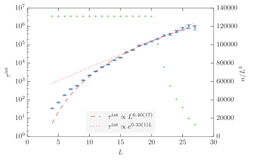
Figure 1: The integrated autocorrelation time $\tau^{\rm int}$ in units of sweeps for the original model with periodic boundary conditions (blue markers; left axis) over the linear lattice size $L$. The dashed and dotted curves are fits with a power law or an exponential law for lattices sizes $L\geq 16$. On the right axis, with green markers, the total number of sweeps $n$ divided by the volume is shown.

Error-weighted nonlinear least-squares fits of a power law, $\tau^{\rm int}\propto L^{\alpha}$, to the actual measured integrated autocorrelation times yield much larger exponents $\alpha\approx 6.40(17)$ that vary a bit around $6.0$ depending on the lattice sizes included in the fits. Also for those fits with acceptable $\chi^{2}\approx 1$ that only include lattices with size $L\geq 16$, fits to an exponential growth with $L$ are of comparable quality, see Figure 1. With least-squares fits and no proper model testing, we cannot distinguish between the two alternatives [25]. In any case, we find that the autocorrelation time grows significantly faster than expected, an effect that may be attributed to free-energy barriers. Such hidden barriers appear for instance in droplet condensation [26], whose analog with the gonihedric Ising model is, however, still unclear.

For each lattice, we performed a maximum number of $n^{\rm max}=2^{17}\,L^{3}=131072\,L^{3}$ sweeps with an upper bound on the computer time of around $500$ hours of real time for each lattice size. All lattices with size $L\leq 20$ finished the desired number of sweeps, the larger lattices were aborted after $500$ hours and collected correspondingly less statistics. The ratio $n/\tau^{\rm int}$ is a measure for the number of effectively uncorrelated data. Although the autocorrelation time increases dramatically with the system size, the simulation of the largest lattice of $V=27^{3}$ spins still effectively flipped more than 250 times between the two phases during the simulation. This is remarkable, given that rare states were suppressed by more than 60 orders of magnitude compared to the most probable states (see the inset of Figure 2).

From our multicanonical data, we have extracted the resulting quantities of interest for different lattice sizes and listed them in Table 3.2, where errors have been extracted by jackknife analysis using $20$ blocks for each lattice size [27].

We find that the inverse temperatures of the specific-heat maximum $\beta^{C_{V}^{\rm max}}$ and of equal peak weights $\beta^{\rm eqw}$ fall nearly together for all lattice sizes. This is accounted for by the fact that the higher-order corrections of order ${\cal O}\left(L^{-4}\right)$ in the scaling law (19) for these quantities collapse due to the exponential degeneracy of the low-temperature phase to induce the same prefactor.

Table 1: Resulting quantities for the gonihedric Ising model (2) with periodic boundary conditions: extremal values for the specific heat $C_{V}^{\rm max}$, Binder’s energy parameter $B^{\rm min}$, with their respective pseudo-critical inverse temperatures $\beta$, and temperatures where peaks of the energy probability density have equal heights and weights for finite lattices with linear length $L$. The finite-lattice interface tension is listed as $\sigma$, the energy of the ordered and disordered phases and their difference as $e_{\rm o},e_{\rm d}$ and $\Delta e$. The infinite lattice limits are listed as parameters of fits whose goodness-of-fit value $Q$ is given. Highlighted in light grey are the datapoints used for fits with only leading order correction (lo). Additional datapoints used for fitting with subleading corrections (so) up to and including order ${\cal O}(L^{-4})$ are marked in dark grey.

$L$	$\beta^{C_{V}^{\rm max}}$	$C_{V}^{\rm max}$	$\beta^{B^{\rm min}}$	$B^{\rm min}$	$\beta^{\rm eqw}$	$\beta^{\rm eqh}$	$\sigma$	$e_{\rm o}$	$e_{\rm d}$	$\Delta e$
08	$0.518228(26)$	$27.061(7)$	$0.513850(27)$	$0.25211(16)$	$0.518244(26)$	$0.514007(23)$	$0.05659(6)$	$-1.43921(13)$	$-0.56223(14)$	$0.87698(11)$
09	$0.524636(24)$	$39.611(6)$	$0.521626(24)$	$0.26024(14)$	$0.524644(24)$	$0.521769(24)$	$0.06240(5)$	$-1.44791(5)$	$-0.56529(8)$	$0.88262(8)$
10	$0.529322(18)$	$55.068(7)$	$0.527159(19)$	$0.27023(12)$	$0.529327(18)$	$0.527463(18)$	$0.067756(29)$	$-1.452764(28)$	$-0.57011(7)$	$0.88265(7)$
11	$0.532894(13)$	$73.766(7)$	$0.531286(13)$	$0.27998(7)$	$0.532897(13)$	$0.531705(12)$	$0.07305(4)$	$-1.455896(28)$	$-0.57525(5)$	$0.88065(4)$
12	$0.535696(13)$	$96.094(8)$	$0.534467(13)$	$0.28847(8)$	$0.535698(13)$	$0.534965(13)$	$0.07804(4)$	$-1.458205(19)$	$-0.57996(5)$	$0.87824(5)$
13	$0.537902(12)$	$122.315(10)$	$0.536941(12)$	$0.29593(8)$	$0.537903(12)$	$0.537383(12)$	$0.08285(4)$	$-1.459850(21)$	$-0.58424(5)$	$0.87561(5)$
14	$0.539662(10)$	$152.801(12)$	$0.538897(10)$	$0.30221(6)$	$0.539663(10)$	$0.539297(9)$	$0.087156(24)$	$-1.461138(15)$	$-0.58795(4)$	$0.87319(4)$
15	$0.541128(9)$	$187.897(12)$	$0.540508(9)$	$0.30756(4)$	$0.541128(9)$	$0.540853(9)$	$0.09105(4)$	$-1.462154(20)$	$-0.591175(23)$	$0.870979(30)$
16	$0.542329(10)$	$227.917(10)$	$0.541820(10)$	$0.31207(5)$	$0.542329(10)$	$0.542114(9)$	$0.09430(4)$	$-1.462961(8)$	$-0.593953(30)$	$0.869009(29)$
17	$0.543326(8)$	$273.174(11)$	$0.542903(8)$	$0.31597(5)$	$0.543326(8)$	$0.543151(8)$	$0.096981(22)$	$-1.463630(8)$	$-0.596392(28)$	$0.867238(24)$
18	$0.544181(9)$	$324.070(9)$	$0.543825(9)$	$0.31923(4)$	$0.544181(9)$	$0.544035(9)$	$0.09928(4)$	$-1.464179(9)$	$-0.598459(27)$	$0.865720(21)$
19	$0.544904(10)$	$380.852(10)$	$0.544602(10)$	$0.32210(4)$	$0.544904(10)$	$0.544781(10)$	$0.10128(4)$	$-1.464630(9)$	$-0.600290(25)$	$0.864339(21)$
20	$0.545510(5)$	$443.910(12)$	$0.545252(5)$	$0.324501(26)$	$0.545511(5)$	$0.545403(5)$	$0.102911(25)$	$-1.465009(6)$	$-0.601844(17)$	$0.863165(16)$
21	$0.546044(7)$	$513.571(12)$	$0.545821(7)$	$0.326601(29)$	$0.546044(7)$	$0.545952(7)$	$0.104440(20)$	$-1.465339(9)$	$-0.603216(21)$	$0.862124(15)$
22	$0.546500(6)$	$590.141(19)$	$0.546306(6)$	$0.328422(24)$	$0.546500(6)$	$0.546420(6)$	$0.10576(4)$	$-1.465615(6)$	$-0.604412(15)$	$0.861203(16)$
23	$0.546914(8)$	$673.971(21)$	$0.546745(8)$	$0.33005(4)$	$0.546914(8)$	$0.546843(8)$	$0.10702(5)$	$-1.465856(7)$	$-0.605491(23)$	$0.860365(20)$
24	$0.547270(9)$	$765.339(21)$	$0.547121(9)$	$0.33152(4)$	$0.547270(9)$	$0.547207(9)$	$0.10819(7)$	$-1.466076(9)$	$-0.606468(24)$	$0.859607(21)$
25	$0.547584(9)$	$864.753(27)$	$0.547452(9)$	$0.33271(4)$	$0.547584(9)$	$0.547528(9)$	$0.10901(5)$	$-1.466270(6)$	$-0.607270(23)$	$0.858999(20)$
26	$0.547856(14)$	$972.36(5)$	$0.547739(14)$	$0.33376(6)$	$0.547856(14)$	$0.547805(14)$	$0.10997(9)$	$-1.466413(11)$	$-0.60798(4)$	$0.85844(4)$
27	$0.548099(14)$	$1088.54(4)$	$0.547994(14)$	$0.33475(6)$	$0.548099(14)$	$0.548053(14)$	$0.11066(10)$	$-1.466578(13)$	$-0.60865(4)$	$0.857927(28)$
lo	$0.551233(10)$	$0.055072(4)L^{3}$	$0.551350(6)$	$0.34729(7)$	$0.551233(10)$	$0.551277(5)$	$0.12037(18)$	$-1.468500(11)$	$-0.61701(7)$	$0.85148(5)$
Q	0.54	0.35	0.72	0.50	0.54	0.90	0.38	0.56	0.56	0.59
so	$0.551331(8)$		$0.551340(27)$		$0.551331(8)$	$0.55134(6)$		$-1.468373(12)$	$-0.61771(6)$
Q	0.95		0.92		0.95	0.93		0.63	0.59

Least-squares fits of the data in Table 3.2 according to the laws in section 2 have been conducted. We have left out the smaller lattices systematically for each fit, until a goodness-of-fit value of at least $Q=0.5$ was found for each observable individually. The same protocol was employed earlier [7] for a reduced time series, where only every $L^{3}$-th measurement was used. There we were not challenging the prefactors of higher-order corrections so the reduced time series was sufficient. We list all the fit parameters obtained for both the full time series and the reduced one in Table 2 along with the quality-of-fit parameters $Q$ and the degrees of freedom left. The inverse transition temperatures in the thermodynamic limit are effectively identical and do not depend on whether we use the reduced or the full dataset or on the precise final averaging procedure. A graphical representation of the best fits is given in Figure 2.

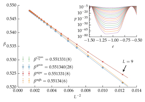
Figure 2: Best fits up to order ${\cal O}(L^{-4})$ obtained for the original model with periodic boundary conditions (cf. Table 2) using the (finite lattice) peak locations for the specific heat $C_{V}^{\rm max}$, Binder’s energy parameter $B^{\rm min}$; or inverse temperatures $\beta^{\rm eqw}$ and $\beta^{\rm eqh}$, where the two peaks of the energy probability density are of same weight or have equal height, respectively. The values for $\beta^{\rm eqw}$ and $\beta^{C^{\rm max}_{V}}$ are indistinguishable in the plot. The inset shows the energy probability density $p(e)$ over $e=E/L^{d}$ at $\beta^{\rm eqh}$ for lattices with linear length $L\in\left\{9,10,\dots,27\right\}$.

Table 2: Resulting parameters of the best fits to the extremal points $\beta$ for the specific heat $C_{V}^{\rm max}$, Binder’s energy parameter $B^{\rm min}$; or inverse temperatures $\beta^{\rm eqw}$ and $\beta^{\rm eqh}$ to laws of the form $\beta(L)=\beta^{\infty}+p_{2}/L^{2}+p_{3}/L^{3}+p_{4}/L^{4}$. Parameters $p_{i}$ not used in the specific fit are marked with –. The error-weighted average over all four inverse temperatures are listed as $\beta^{\rm av}$, whereas $\beta^{\rm av}_{\text{w/o eqw}}$ is the average, where $\beta^{\rm eqw}$ is left out, because it is strongly correlated with $\beta^{C^{\rm max}_{V}}$, and would effectively weight this value twice.

${\cal O}$	Eq.	$L_{\rm min}$	$\beta^{\infty}$	$p_{2}$	$p_{3}$	$p_{4}$	$Q$	dof
reduced time series, linear fit
$\beta^{C_{V}^{\rm max}}(L)$	(19)	16	0.551221(11)	$-2.281(5)$	–	–	0.54	10
$\beta^{B^{\rm min}}(L)$	(20)	13	0.551347(7)	$-2.4373(24)$	–	–	0.79	13
$\beta^{\rm eqw}(L)$	(19)	16	0.551221(11)	$-2.281(5)$	–	–	0.54	10
$\beta^{\rm eqh}(L)$	(19)	5	0.551331(21)	$-2.366(6)$	–	–	0.96	21
$\beta^{\rm av}$			0.551291(7)	1.313527(12)
$\beta^{\rm av}_{\text{w/o eqw}}$			0.551311(7)	1.313493(12)
full time series, linear fit
$\beta^{C_{V}^{\rm max}}(L)$	(19)	17	0.551233(10)	$-2.287(5)$	–	–	0.54	9
$\beta^{B^{\rm min}}(L)$	(20)	13	0.551350(6)	$-2.4389(19)$	–	–	0.72	13
$\beta^{\rm eqw}(L)$	(19)	17	0.551233(10)	$-2.287(5)$	–	–	0.54	9
$\beta^{\rm eqh}(L)$	(19)	12	0.551277(5)	$-2.3478(16)$	–	–	0.90	14
$\beta^{\rm av}$			0.551293(5)	1.313524(9)
$\beta^{\rm av}_{\text{w/o eqw}}$			0.551300(5)	1.313511(9)
full time series, up to ${\cal O}\left(L^{-3}\right)$
$\beta^{B^{\rm min}}(L)$	(20)	11	0.551403(14)	$-2.494(11)$	0.65(12)	–	0.59	14
$\beta^{\rm eqh}(L)$	(19)	12	0.551271(17)	$-2.342(15)$	0(0.2)	–	0.87	13
$\beta^{\rm av}$			0.551269(10)	1.313565(17)
$\beta^{\rm av}_{\text{w/o eqw}}$			0.551288(10)	1.313532(17)
full time series, up to ${\cal O}\left(L^{-4}\right)$
$\beta^{C_{V}^{\rm max}}(L)$	(19)	9	0.551331(8)	$-2.371(4)$	–	$\hphantom{-}16.9(4)$	0.95	16
$\beta^{B^{\rm min}}(L)$	(20)	9	0.551340(28)	$-2.39(4)$	$-1.6(8)$	$\hphantom{-}13(4)$	0.92	15
$\beta^{\rm eqw}(L)$	(19)	9	0.551331(8)	$-2.371(4)$	–	$\hphantom{-}17.0(4)$	0.95	16
$\beta^{\rm eqh}(L)$	(19)	12	0.55134(6)	$-2.47(11)$	$\hphantom{-}2.8(2.4)$	$-18(15)$	0.95	12
$\beta^{\rm av}$			0.551332(8)	1.313457(14)
$\beta^{\rm av}_{\text{w/o eqw}}$			0.551332(8)	1.313456(14)

Since the inverse temperatures $\beta^{\rm eqw}$ and $\beta^{C_{V}^{\rm max}}$ are obviously strongly correlated, we leave out the former and average over $\beta^{C_{V}^{\rm max}},\beta^{B^{\rm min}}$, and $\beta^{\rm eqh}$, neglecting cross-correlations [28] between those. Our best estimate of the inverse transition temperature is then given by

$$\beta^{\infty} =0.551\,332(8)$$ original model, periodic bc, (34)

which accounts for the higher-order scaling corrections up to ${\cal O}\left(L^{-4}\right)$.

Although the inverse transition temperatures do not change, we employ the full data set. The reason is that the error on $\beta^{\rm eqh}$ becomes smaller for the time series that uses the full, correlated data set. This is attributed to the fact that the observable relies on the statistics in single bins of the energy histogram, which in total becomes smoother when using more, correlated measurements. The same argument is valid for the calculation of the interface tension (33), for which the best fit with corrections of order ${\cal O}(L^{-2})$ yields a value of

$$\hat{\sigma}=0.12037(18)$$ original model, periodic bc. (35)

Moments of the energy in the pure ordered and disordered phases are also expected to become more accurate using the full data set, since autocorrelation times in the pure phases are then significantly smaller than $\tau^{\rm int}$ for the full energy range (see below). By fitting the scaling law (27) to these moments, one obtains the latent heat in the infinite-volume limit,

$$\Delta\hat{e}=0.85148(5)$$ original model, periodic bc. (36)

Taking a careful look at the scaling laws in section 2, we find that the prefactors of the scaling corrections only depend on the moments of the energy or their differences. We have two methods at hand to test the self-consistency of our simulations. Firstly, since the statistics of the observables are very high, we can retrieve the prefactors of the corrections as parameters of (nonlinear) least-squares-fits with all corrections up to and including ${\cal O}(L^{-4})$. Secondly, from multicanonical simulations we get estimators (30) of the energy moments, allowing a direct computation of those prefactors.

In addition, we carried out independent canonical simulations for the original model under periodic boundary conditions for very large lattices. The goal was to get independent measurements of the moments of the energy in the ordered and disordered phases. Here we prepared the system in the appropriate phase and performed the simulations at a fixed temperature $\beta=0.5513$, near the transition temperature, exploiting the fact that in canonical simulations, for large lattices, flips between the two phases are extremely unlikely. Of course, this was only possible after having determined the transition temperature with high accuracy by the multicanonical simulations.

The quality of the canonical measurements and estimators on the energy and the specific heat are summarized in Table 3. The autocorrelation times within the phases are significantly smaller, because the system does not traverse suppressed, improbable states between the phases. The statistical error has again been retrieved by jackknife analysis. For lattices with size $L\geq 32$, physical quantities indicate no further dependence on the lattice size within the error. Therefore we can safely take the error-weighted averages over energy moments and their differences for those lattices. The multicanonical and the canonical estimates of energetic moments agree astonishingly well.

With use of the energy moments from both simulations, we can challenge the prefactors in the finite-size scaling laws numerically by comparing the numerical values for the fit parameters to the theoretically expected prefactors in terms of the energy moments. The results of this cross-check are collected in Table 4.

Table 3: Quality and resulting quantities of the canonical simulations. In the time series of $n_{\rm meas}=1048576$ measurements we found autocorrelation times $\tau<7$ (in units of measurements), leading to approximately $n$ uncorrelated measurements. The energy $\hat{e}_{\rm o/d}$ and the specific heat $\hat{C}_{\rm o/d}$ in the different phases have been measured by preparing two independent systems for each respective phase at inverse temperature $\beta=0.5513$. We give the error-weighted average over lattices $L\geq 32$, where the dependence on the lattice size is smaller than the statistical error. The last line gives infinite-volume limits from the multicanonical simulations for comparison.

$L$	$n$	$\hat{e}_{o}$	$\hat{e}_{d}$	$\Delta\hat{e}$	$\hat{C}_{o}$	$\hat{C}_{d}$	$\Delta\hat{C}$
16	149796	$-1.468406(29)$	$-0.61804(13)$	0.85036(21)	0.1645(5)	0.861(4)	0.696(6)
32	174762	$-1.468362(10)$	$-0.61741(4)$	0.85095(6)	0.1645(6)	0.8464(29)	0.682(5)
48	149796	$-1.468360(6)$	$-0.617382(19)$	0.850978(30)	0.1658(5)	0.8445(27)	0.679(5)
64	174762	$-1.468367(6)$	$-0.617401(15)$	0.850966(24)	0.1656(6)	0.847(4)	0.681(6)
average $(L\geq 32)$		$-1.468364(4)$	$-0.617396(11)$	0.850968(18)	0.16534(30)	0.8458(18)	0.6805(27)
multicanonical		$-1.468373(12)$	$-0.61771(6)$	0.85148(5)	0.16414(15)	0.8410(12)	0.6769(17)

Employing the scaling relation for the specific-heat maximum (22), we can calculate $\Delta\hat{e}$ from the fit parameter of the leading contribution. Using our estimate of $\beta^{\infty}=0.551\,332(8)$, we get $\Delta\hat{e}=0.85130(7)$, very close to our estimate $0.850968(18)$ from the moments of the canonical simulations. The leading correction to the specific-heat ansatz (22) has a prefactor which computes to $0.2197(17)$ from the canonical moments. The fits find $0.17(6)$, which is compatible, if not quite accurate.

The minimum of the Binder parameter (23) for the infinite lattice is found to be $0.34729(7)$ from the direct fit of our multicanonical data which agrees within error bars with $0.34723(9)$ from the canonical and $0.347(4)$ from the multicanonical energy moments. The first correction in Eq. (24) yields a value of $-9.195(14)$ when inserting the energy moments from the multicanonical simulation. The fits find $-9.12(4)$ which is very close.

Table 4: Resulting prefactors of the finite-size scaling corrections of the original model, retrieved by fitting the ansatz, compared to direct calculations from estimators for the energy $\hat{e}_{\rm o/d}$ and specific heat $\hat{C}_{\rm o/d}$ of the ordered and disordered phases. In the multicanonical simulations these moments were determined by finite-size scaling of $e_{\rm o/d}(L),c_{\rm o/d}(L)$; and in the canonical case by measuring time series directly at $\beta=0.5513\simeq\beta^{\infty}$.

input	$\Delta\hat{e}$	$\frac{3\ln(2)}{\Delta\hat{e}}$	$\frac{2\ln(\hat{e}_{\rm o}/\hat{e}_{\rm d})}{\Delta\hat{e}}$	$\frac{\ln(\hat{C}_{\rm d}/\hat{C}_{\rm o})}{2\Delta\hat{e}}$	$B^{\rm min}_{L\rightarrow\infty}$
fit on $C^{\rm max}_{V}(L)$	0.85130(7)	–	–	–	–
fit on $B^{\rm min}(L)$	–	–	–	–	0.34729(7)
fit on $\beta^{C^{\rm max}_{V}}(L)$	0.8771(14)	$2.371(4)$	–	–	–
fit on $\beta^{B^{\rm min}}(L)$	0.871(14)	$2.39(4)$	1.6(8)	–	–
fit on $\beta^{\rm eqw}(L)$	0.8770(14)	$2.371(4)$	–	–	–
fit on $\beta^{\rm eqh}(L)$	0.84(4)	$2.47(11)$	–	2.8(2.4)	–
fit on $\beta^{C^{\rm max}_{V}}-\beta^{B^{\rm min}}$	–	–	2.03469(7)	–	–
fit on $\beta^{C^{\rm max}_{V}}-\beta^{\rm eqh}$	–	–	–	0.892(14)	–
energy moments from simulations …
…multicanonical	0.85148(5)	$2.44215(15)$	2.03649(27)	0.9594(10)	0.347(4)
…canonical	0.850968(18)	$2.44362(6)$	2.03625(6)	0.9591(16)	0.34723(9)

The coefficient of the leading correction apparent for all inverse temperatures, $p_{2}=3\ln(2)/\Delta\hat{e}$, agrees reasonably well for the fits on $\beta^{B^{\rm min}}$ and $\beta^{\rm eqh}$ (cf. Table 4). The fits on $\beta^{\rm eqw}$ and $\beta^{C^{\rm max}_{V}}$ yield a slope of $2.371({4})$ which within error bars is slightly off from the value of our best estimate of $2.44362(6)$ from the energy moments. The relative error between the two values is very small though, around $3\%$, which is acceptable given that the leading contribution probably accounts for the omitted higher-order contributions with different sign and that we have neglected all exponential corrections.

The second leading correction of order ${\cal O}(L^{-3})$ of $\beta^{B^{\rm min}}$ has a prefactor of the form $2\ln(\hat{e}_{\rm o}/\hat{e}_{\rm d})/\Delta\hat{e}$, which we expect to have a value of $2.03625(6)$ from the energy moments. The corrections of fourth order to $\beta^{B^{\rm min}},\beta^{C^{\rm max}_{V}}$ and $\beta^{\rm eqw}$ are supposed to be identical from the analytical expansion in section 2. The fits of the inverse temperatures $\beta^{C^{\rm max}_{V}}$ and $\beta^{\rm eqw}$ in Table 2 suggest a value around $17$ for the ${\cal O}(L^{-4})$ contribution. For the lattice sizes accessible to the multicanonical approach, that is of the same absolute order of magnitude (but different sign) compared to the third-order contribution. Therefore they should, in principle, compensate each other. This is reflected by the fact that the second-order contribution $p_{2}$ of $\beta^{B^{\rm min}}$ is closest to the expected one. In accordance, fitting the observable to the law $\beta^{\infty}+p_{2}/L^{2}+p_{3}/L^{3}$ gives a prefactor $p_{3}=0.65(12)$ with the wrong sign compared to the theoretical prediction (20), compensating the next contribution. We therefore also looked at the fit including the fourth term of order ${\cal O}(L^{-4})$. Not taking the explicit values too seriously, we find $p_{3}=-1.6(8),\,p_{4}=13(4)$, which reflect qualitatively the compensation of those contributions for our lattice sizes at hand. Overall, we must conclude that least-squares fitting cannot be pushed any further given our statistics.

The observation that $\beta^{C^{\rm max}_{V}}$ and $\beta^{B^{\rm min}}$ have the same ${\cal O}(L^{-4})$-contribution can be exploited (implicitly also making use of the cross-correlations) by looking at their difference. Here, we expect from (19) and (20) a remainder of $2\ln(\hat{e}_{\rm o}/\hat{e}_{\rm d})/L^{3}\Delta\hat{e}+{\cal O}(L^{-5})$ for the scaling. In fact, fitting the difference gives a prefactor $2.03469(7)$, in excellent agreement with $2.03625(6)$ from the formula, where the relative error between the two is less than $0.1\%$.

The difference $\beta^{C^{\rm max}_{V}}-\beta^{\rm eqh}$ should give the third correction to $\beta^{\rm eqh}$, which reads $p_{3}=\ln(\hat{C}_{\rm d}/\hat{C}_{\rm o})/2\Delta\hat{e}$. The fit yields $0.892(14)$ with $Q=0.98$ and $8$ degrees of freedom left, which differs from $0.9594(10)$ by about $7\%$.

Finally, we can also compare the numerical values for the correction to the energies via (27). For $\hat{e}_{\rm o}$, we find a prefactor of $1.329(5)$ from the specific heat $\hat{C}_{\rm o}$, compared to the value of $1.397(5)$, for $\hat{e}_{\rm d}$ a value of $6.80(3)$ compared to $6.09(4)$, which is roughly $10\%$ off.

The overall consistency of our results is very good, given that we neglected all exponential corrections. No estimates for the prefactors differ by more than $10\%$, and the various estimates of the inverse transition temperature are insensitive to the actual fitting protocol we use. This clearly demonstates that the first correction terms are properly predicted by the simple two-state model even in the case of models with an exponential degeneracy of the low-temperature phase.

The earlier canonical Monte Carlo simulations of the original plaquette model yielded values of $\beta^{\infty}=0.50(1)$ [8] and more recently canonical simulations of the dual model (3) gave $\beta^{\infty}=0.510(2)$ [10]. Another previous estimate for the infinite-lattice inverse transition temperature, reported by Baig et al. [9] from canonical simulations using fixed boundary conditions, $\beta^{\infty}=0.54757(63)$, is much closer to the results here.

We therefore measured the inverse transition temperature again using multicanonical simulations for both the dual model (3) under periodic boundary conditions and the original model (2) with fixed boundary conditions. We resolve those inconsistencies, as we show in the following.

3.3 Dual model with periodic boundary conditions

For the dual model, we performed a number of $n^{\rm max}=4\times 10^{6}$ sweeps and took measurements every sweep for even lattices up to $L=24$. The inverse temperatures of the dual model were fitted to laws with the leading correction of order ${\cal O}(L^{-2})$, which should be well covered by our data. The best fits on the inverse temperatures are shown in Figure 3, where we used the data in Table 3.3 that also lists the other quantities of interest.

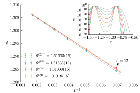
Figure 3: Best fits obtained for the dual model with periodic boundary conditions using the (finite lattice) peak locations for the specific heat $C_{V}^{\rm max}$, Binder’s energy parameter $B^{\rm min}$; or inverse temperatures $\beta^{\rm eqw}$ and $\beta^{\rm eqh}$, where the two peaks of the energy probability density are of same weight or have equal height, respectively. The inset shows the energy probability density $p(e)$ over $e=E/L^{d}$ at $\beta^{\rm eqh}$ for lattices of linear size $L\in\left\{12,14,\dots,24\right\}$.

Since the inverse temperatures $\beta^{\rm eqw}$ and $\beta^{C_{V}^{\rm max}}$ are again obviously strongly correlated, we leave out the former and average over $\beta^{C_{V}^{\rm max}},\beta^{B^{\rm min}}$, and $\beta^{\rm eqh}$, neglecting cross-correlations [28] between those. We then find the error weighted averages,

$$\beta^{\infty}_{\rm dual} =1.313\,28(12)$$ dual model, periodic bc, (37)

for the inverse transition temperatures of the models. The error is taken as the smallest error of the contributing estimates.

The temperature $\beta^{\infty}_{\rm dual}$ of the dual model is related to the temperature in the original model, $\beta^{\infty}$, by the duality transformation

$$\beta^{\infty}=-\ln\left(\tanh\left(\frac{\beta^{\infty}_{\text{dual}}}{2}\right)\right).$$ (38)

Applying standard error propagation, we retrieve a value of

$$\beta^{\infty} =0.551\,43(7)\qquad$$ from duality, periodic bc (39)

for the original model. This agrees very well with $0.551\,332(8)$, obtained from the direct simulation, considering that higher-order corrections in the dual model are omitted and additional exponential corrections [15, 16, 18] in the finite-size scaling were ignored completely for both models.

We argue that the earlier estimates on the transition temperature were clearly hampered by strong hysteresis effects. Apart from the locations of the hysteresis branches being cooling-rate dependent, it is hard to estimate the transition temperature reliably from their locations. This is illustrated in Figure 4, where the multicanonical data of the dual model is located between the two hysteresis branches. Such effects are very difficult to tackle using canonical Monte Carlo data, as already remarked on by the authors of Ref. [10].

For the interface tension (33) of the dual model we find $\sigma=0.1214(13)$. This value agrees very well with the interface tension of the original model, $\sigma=0.12037(18)$, which raises interesting questions about the duality of the model.

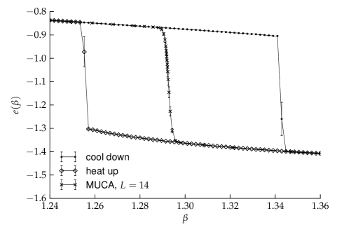
Figure 4: Strong hysteresis effects in the dual gonihedric Ising model with periodic boundary conditions. The linear lattice size is $L=14$ for comparison with Fig. 10 of Ref. [10]. One can see that heating the system up (decreasing the inverse temperature $\beta$) or cooling it down (increasing $\beta$) can lead to strong hysteresis effects in the energy. Our multicanonical data lies in between both branches of the hysteresis curve, but not in the centre, as one may heuristically assume.

3.4 Original plaquette model with fixed boundary conditions

The remaining open question is the difference between our inverse transition temperature compared to the value in the same model under fixed boundary conditions. In the thermodynamic limit, we expect a system to be independent of its boundary conditions, since the boundaries grow like a surface, whereas the system size grows with the volume. We therefore reinvestigated the model (2) using the multicanonical algorithm for such fixed boundary conditions.

Table 6: Extremal points of the gonihedric Ising model (2) for the specific heat $C_{V}^{\rm max}$, Binder’s energy parameter $B^{\rm min}$, with their respective pseudo-critical inverse temperatures $\beta$ for finite lattices with linear length $L$ contained in a box with fixed boundary conditions. For each lattice size, a number of $n_{\rm prod}=10^{6}$ measurements were taken. Errors have been calculated with jackknife error estimation using $20$ blocks.

$L$	$\beta^{C_{V}^{\rm max}}$	$C_{V}^{\rm max}$	$\beta^{B^{\rm min}}$	$B^{\rm min}$	$\beta^{\rm eqw}$	$\beta^{\rm eqh}$	$\sigma$	$e_{\rm o}$	$e_{\rm d}$	$\Delta e$
08	0.44699(14)	5.29(4)	0.44233(13)	0.63030(26)	0.4475(18)	0.4479(8)	0(0.002)	$-1.67(5)$	$-1.29(6)$	0.387(7)
09	0.45794(13)	7.63(8)	0.45488(14)	0.6305(4)	0.4594(12)	0.4577(11)	0(0.003)	$-1.65(4)$	$-1.28(5)$	0.379(10)
10	0.46715(15)	11.08(12)	0.46510(16)	0.6293(5)	0.4678(6)	0.46683(26)	0(0.003)	$-1.623(21)$	$-1.230(29)$	0.394(9)
11	0.47465(14)	15.81(14)	0.47323(14)	0.6273(4)	0.4752(5)	0.47403(25)	0.0044(8)	$-1.62(4)$	$-1.21(6)$	0.410(20)
12	0.48097(14)	22.70(26)	0.47995(14)	0.6234(6)	0.48136(19)	0.4803(4)	0.0060(13)	$-1.625(9)$	$-1.192(19)$	0.433(11)
13	0.48629(9)	31.56(30)	0.48552(9)	0.6197(6)	0.48653(9)	0.48566(9)	0.0072(14)	$-1.6230(7)$	$-1.1654(25)$	0.4575(27)
14	0.49086(8)	43.7(5)	0.49027(9)	0.6146(7)	0.49099(11)	0.49020(27)	0.0090(7)	$-1.620(8)$	$-1.129(17)$	0.490(9)
15	0.49483(13)	56.8(8)	0.49435(13)	0.6116(9)	0.49490(17)	0.49429(12)	0.0097(11)	$-1.612(14)$	$-1.104(28)$	0.508(14)
16	0.49825(11)	75.2(8)	0.49786(11)	0.6059(8)	0.49830(11)	0.49778(10)	0.0119(4)	$-1.6108(5)$	$-1.080(4)$	0.531(4)
17	0.50126(7)	92.6(8)	0.50093(7)	0.6043(7)	0.50129(7)	0.50090(19)	0.0125(20)	$-1.6046(5)$	$-1.0664(27)$	0.5382(25)
18	0.50410(6)	115.3(11)	0.50383(6)	0.6008(8)	0.50412(6)	0.50381(24)	0.0135(19)	$-1.59885(24)$	$-1.0487(28)$	0.5501(28)
19	0.50648(8)	141.9(12)	0.50625(8)	0.5969(8)	0.50649(8)	0.50620(14)	0.0147(15)	$-1.59286(27)$	$-1.0311(24)$	0.5618(24)
20	0.50866(10)	167.3(16)	0.50846(10)	0.5963(10)	0.50867(10)	0.50841(12)	0.0156(13)	$-1.58807(27)$	$-1.0248(30)$	0.5633(29)
21	0.51063(8)	200.7(19)	0.51046(8)	0.5930(9)	0.51064(8)	0.51039(7)	0.01706(26)	$-1.5828(4)$	$-1.0106(27)$	0.5722(28)
22	0.51258(6)	235.1(21)	0.51243(6)	0.5914(9)	0.51259(6)	0.51237(5)	0.0173(12)	$-1.57837(20)$	$-1.0024(26)$	0.5759(26)
23	0.51433(7)	275.6(24)	0.51420(7)	0.5889(10)	0.51433(7)	0.51415(7)	0.01905(26)	$-1.57402(20)$	$-0.9920(27)$	0.5820(26)
24	0.51586(6)	317(4)	0.51574(6)	0.5879(11)	0.51586(6)	0.51568(6)	0.0193(6)	$-1.57031(14)$	$-0.9864(28)$	0.5839(28)
25	0.51728(7)	368.6(21)	0.51718(7)	0.5847(7)	0.51729(7)	0.51716(6)	0.0200(10)	$-1.56641(24)$	$-0.9750(18)$	0.5914(17)
26	0.51853(6)	422.2(28)	0.51843(6)	0.5827(8)	0.51853(6)	0.51837(15)	0.0207(11)	$-1.56259(18)$	$-0.9670(20)$	0.5956(20)
27	0.51985(7)	472(4)	0.51977(7)	0.5830(8)	0.51985(7)	0.51971(6)	0.0210(14)	$-1.55980(25)$	$-0.9656(20)$	0.5942(20)
28	0.52084(6)	543(5)	0.52077(6)	0.5795(12)	0.52084(6)	0.52073(9)	0.0220(4)	$-1.55660(11)$	$-0.9544(28)$	0.6022(28)
29	0.52198(24)	603(12)	0.52191(24)	0.5796(23)	0.52198(24)	0.52190(13)	0.023(5)	$-1.5538(9)$	$-0.953(6)$	0.601(7)
$\infty$	0.55119(11)	0.0327(6)$L^{3}$	0.55146(7)	0.5444(14)	0.55119(12)	0.55152(12)	0.0281(7)	$-1.4782(27)$	$-0.790(4)$	0.694(4)
$Q$	0.53	0.53	0.56	0.59	0.52	0.53	0.99	0.49	0.73	0.50

For our simulations we enclosed $L^{3}$ free spins in a larger cube with frozen outer planes, so the whole system contained $(L+2)^{3}$ spins. Our results are listed in Table 6. We performed linear regression on the peak locations $\beta(L)$ of the specific heat and Binder’s parameter according to the law

$$\beta^{\infty}=\beta(L)+\frac{a_{1}}{L}+\frac{a_{2}}{L^{2}}$$ (40)

that was also used by Baig et al. [9], and fitted the inverse temperatures. The statistical errors of the constant $a_{2}$ turned out to be of the same order as the value itself, therefore we set $a_{2}=0$ for the fits in Table 6, intentionally neglecting the contribution $\mathcal{O}(L^{-2})$. The best fits and the energy probability density are shown in Figure 5 and the weighted average of inverse transition temperatures is given by:

$$\beta^{\infty} =0.551\,38(5)\qquad \textrm{original model, fixed bc}.$$ (41)

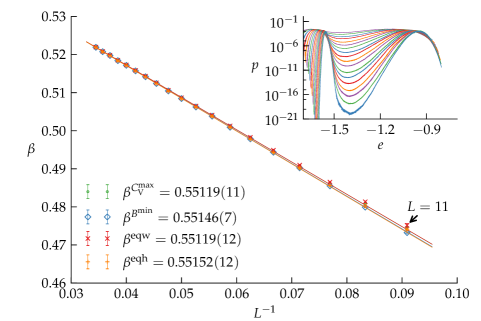
Figure 5: Best fits obtained for the gonihedric Ising model using fixed boundary conditions using the (finite lattice) peak locations for the specific heat $C^{\rm max}$, Binder’s energy parameter $B_{\rm min}$. The inset shows the energy probability density $p(e)$ over $e=E/L^{3}$ at $\beta^{\rm eqh}$ for lattices with a number of $L\in\left\{11,12,\dots,29\right\}$ free spins in each dimension.

This estimate of the inverse transition temperature is thus in excellent agreement with the other results obtained here from multicanonical simulations with periodic boundary conditions for the gonihedric Ising model $\beta^{\infty}=0.551\,332(8)$ and the dual model $\beta^{\infty}=0.551\,43(7)$.

Direct comparison to Ref. [9] shows that while inverse transition temperatures are reproduced, the extremal values of observables are not. The following observations may help to clarify the deviations. The authors of Ref. [9] simulated the system by applying periodic boundary conditions and fixing one plane parallel to the $xy$-, $yz$- and $zx$-planes each. If their simulation box consisted of a total number of $\hat{L}^{3}$ spins, they simulated $(\hat{L}-1)^{3}$ free spins. Thus our data with lattices of linear length $L$ has to be compared to their data with $\hat{L}=L+1$. Also, their specific heat and magnetic susceptibility $\hat{\chi}=\beta\hat{L}^{-d}\left(\langle M^{2}\rangle-\langle M\rangle^{2}\right)$ have to be multiplied by a factor of $(L+1)^{3}/L^{3}$ to be comparable with our normalization, since these quantities are proportional to the inverse system volume. Here, $M=\sum_{i}\sigma_{i}$ is the total magnetization, which for fixed boundary conditions is a well defined order parameter.

Binder’s energy parameter has no explicit volume-dependence by design, but it is sensitive to offsets in the energy, which cancel in the specific heat. Our values of the Binder parameter minima differ significantly from [9]. However, if we shift our measured energies $E$ to get $\hat{E}=E-1.5\hat{L}^{2}=E-1.5(L+1)^{2}$ and calculate Binder’s parameter (6) with $\hat{E}$ instead of $E$, our measurements reproduce those of [9] very well. The energy $E$ of the system can be written in terms of the number of plaquettes with an even or odd number of parallel aligned spins, $n_{+}$ or $n_{-}$,

$$E(\beta)=-\frac{1}{2}\left(n_{+}(\beta)-n_{-}(\beta)\right).$$ (42)

Since we measure the same cumulant values for shifted energies $\hat{E}$, in Ref. [9] an additional number of $\hat{n}_{+}=n_{+}+3\hat{L}^{2}$ plaquettes contribute to the system’s energy because energetic contributions from the fixed planes, where all spins are aligned, were included.

Table 7: Values for comparison with Ref. [9], with the hat denoting the observables as calculated by Baig et al. Linear lattice lengths are $\hat{L}=L+1$, with $L$ being the number of free spins in each direction. The specific heat $\hat{C}_{V}^{\rm max}=L^{3}/(L+1)^{3}C_{V}^{\rm max}$, Binder’s parameter $\hat{B}_{\rm min}=1.0-\langle\hat{E}^{4}\rangle/3\langle\hat{E}^{2}\rangle^{2}$ with $\hat{E}=E-1.5\hat{L}^{2}$. The inverse temperatures $\beta$ are the same for their data and ours. Magnetic susceptibilities $\hat{\chi}^{\rm max}=L^{3}/(L+1)^{3}\chi^{\rm max}$ are listed as well.

$L$	$\hat{L}$	$\beta^{\hat{C}_{V}^{\rm max}}$	$\hat{C}_{V}^{\rm max}$	$\beta^{\hat{B}^{\rm min}}$	$\hat{B}^{\rm min}$	$\beta^{\hat{\chi}^{\rm max}}$	$\hat{\chi}^{\rm max}$
9	10	0.45794(13)	5.56(6)	0.45527(14)	0.63964(29)	0.45690(14)	6.86(9)
11	12	0.47465(14)	12.18(11)	0.47338(14)	0.63555(30)	0.47438(14)	16.37(15)
13	14	0.48629(9)	25.27(24)	0.48559(9)	0.6282(5)	0.48621(9)	36.5(4)
14	15	0.49086(8)	35.5(4)	0.49032(9)	0.6234(6)	0.49083(9)	52.9(7)
17	18	0.50126(7)	78.0(6)	0.50096(7)	0.6133(6)	0.50125(7)	126.2(1.2)
19	20	0.50648(8)	121.7(1.0)	0.50626(8)	0.6062(7)	0.50648(8)	206.9(1.9)

For direct comparison, the resulting quantities are listed in Table 7 after applying all corrections, showing that our data is then in very good agreement with Ref. [9]. For completeness we include here also our data for the magnetic susceptibility $\hat{\chi}$. The deviation from the fitting results in Ref. [9] simply stems from the fact that our simulations are performed with the multicanonical method that allows a finite-size scaling analysis with more and significantly larger lattice sizes.

The interface tension as a function of the linear lattice size (33) is extracted and its infinite-volume limit yields a value of $\sigma=0.0281(7)$ where we allowed corrections of order ${\cal O}(L^{-2})$ in the fits. Note that this value is about four times smaller than that for the same model with periodic boundary conditions.

4 Summary

We simulated the plaquette gonihedric Ising model and its dual to shed some light on discrepancies in the recent literature on the reported value(s) of the first-order phase transition temperature. High-precision results from multicanonical simulations forced us to review the traditional scaling ansatz for first-order finite-size corrections by taking the exponential low-temperature phase degeneracy of the model into account. The leading correction in such circumstances is then no longer proportional to the inverse volume of the system, ${\cal O}\left(L^{-3}\right)$, but is rather ${\cal O}\left(L^{-2}\right)$. With this finite-size scaling ansatz, our simulations with periodic boundary conditions produced consistent results for both the original formulation of the model as well as its dual representation. Since our results also differed from earlier simulations using fixed boundary conditions, where the leading corrections are now ${\cal O}\left(L^{-1}\right)$, we carried out multicanonical simulations of the gonihedric Ising model with these boundary conditions too. The resulting inverse transition temperature was fully consistent with the value found using periodic boundary conditions when larger lattices were included, and hopefully settle once and for all enduring inconsistencies. Interestingly, we do find different values for the latent heat for different boundary conditions, $\Delta\hat{e}=0.694(4)$ in the case of fixed boundary conditions compared to $\Delta\hat{e}=0.850968(18)$ for periodic boundaries. That the latent heat may be dependent on the boundary conditions has been observed earlier for the $q$-states Potts model [19].

The main resulting physical quantities that characterize the first-order phase transition are summarized in Table 8 for the different models and boundary conditions in our simulations. We find an overall consistent value for the inverse transition temperature of

$$\beta^{\infty}=0.551\,334(8)$$ (43)

and we measure the interface tension of the original model and its dual for the first time. We find values of $\sigma=0.12037(18)$ and $\sigma=0.1214(13)$ for the original and dual model with periodic boundary conditions, respectively. The interface tension of the original model with fixed boundary conditions is found to be much smaller, $\sigma=0.0281(7)$.

Table 8: Overview of resulting quantities of the infinite systems.

model	bc	$\beta^{\infty}$	$\hat{e}_{\rm o}$	$\hat{e}_{\rm d}$	$\Delta\hat{e}$	$\hat{\sigma}$
original (2)	periodic	0.551332(8)	$-1.468364(4)$	$-0.617396(11)$	0.850968(18)	0.12037(18)
dual (3)	periodic	0.55143(7)	$-1.37644(21)$	$-0.88227(19)$	0.49402(26)	0.1214(13)
		[$\beta^{\infty}_{\rm dual}=1.31328(12)$]
original (2)	fixed	0.55138(5)	$-1.4782(27)$	$-0.790(4)$	0.694(4)	0.0281(7)

Any model with an exponentially degenerate low-temperature phase will display the modified scaling at a first-order phase transition we have delineated for the three-dimensional gonihedric model and its dual here. Apart from higher-dimensional variants of the gonihedric model or its dual, there are numerous other models in which the scenario could be realized. Examples range from ANNNI models [29] to topological “orbital” models in the context of quantum computing [30] which all share an extensive ground-state degeneracy. Among the orbital models for transition metal compounds, a particularly promising candidate is the three-dimensional classical compass or $t_{2g}$ orbital model where a highly degenerate ground state is well known and the signature of a first-order transition into the disordered phase has recently been found numerically [31].

Other systems, such as the three-dimensional Ising antiferromagnet on an FCC lattice, have an exponentially degenerate number of ground states but a small number (6 in the case of the FCC Ising antiferromagnet) of true low-temperature phases. Nonetheless, they do possess an exponentially degenerate number of low-energy excitations so, depending on the nature of the growth of energy barriers with system size, an effective modified scaling could still be seen at a first-order transition for the lattice sizes accessible in typical simulations. The crossover to the true asymptotic (standard) scaling would then only appear for very large lattices. Indeed, previous simulations appear to have found non-standard scaling for the first-order transition in the three-dimensional Ising antiferromagnet on an FCC lattice [32].

Acknowledgment

This work was supported by the Deutsche Forschungsgemeinschaft (DFG) through the Collaborative Research Centre SFB/TRR 102 (project B04) and by the Deutsch-Französische Hochschule (DFH-UFA) under Grant No. CDFA-02-07.

References

References

- [1] R. V. Ambartzumian, G. K. Savvidy, K. G. Savvidy, G. S. Sukiasian, Phys. Lett. B 275 (1992) 99; G. K. Savvidy, K. G. Savvidy, Mod. Phys. Lett. A 08 (1993) 2963; G. K. Savvidy, K. G. Savvidy, Int. J. Mod. Phys. A 08 (1993) 3993.
- [2] G. K. Savvidy, F. J. Wegner, Nucl. Phys. B 413 (1994) 605; G. K. Savvidy, K. G. Savvidy, Phys. Lett. B 324 (1994) 72; G. K. Bathas, E. Floratos, G. K. Savvidy, K. G. Savvidy, Mod. Phys. Lett. A 10 (1995) 2695; G. K. Savvidy, K. G. Savvidy, P. G. Savvidy, Phys. Lett. A 221 (1996) 233.
- [3] D. A. Johnston, A. Lipowski, R. K. P. C. Malmini, in Rugged Free Energy Landscapes: Common Computational Approaches to Spin Glasses, Structural Glasses and Biological Macromolecules, ed. W. Janke, Lecture Notes in Physics 736 (Springer, Berlin, 2008), p. 173.
- [4] D. Espriu, M. Baig, D. A. Johnston, R. K. P. C. Malmini, J. Phys. A 30 (1997) 405.
- [5] A. Lipowski, J. Phys. A 30 (1997) 7365; A. Lipowski, D. A. Johnston, J. Phys. A 33 (2000) 4451; A. Lipowski, D. A. Johnston, Phys. Rev. E 61 (2000) 6375; A. Lipowski, D. A. Johnston, D. Espriu, Phys. Rev. E 62 (2000) 3404; M. Swift, H. Bokil, R. Travasso, A. Bray, Phys. Rev. B 62 (2000) 11494; C. Castelnovo, C. Chamon, D. Sherrington, Phys. Rev. B 81 (2010) 184303.
- [6] R. Pietig, F. Wegner, Nucl. Phys. B 466 (1996) 513; R. Pietig, F. Wegner, Nucl. Phys. B 525 (1998) 549.
- [7] M. Mueller, W. Janke, D. A. Johnston, Phys. Rev. Lett. 112 (2014) 200601.
- [8] D. A. Johnston, R. K. P. C. Malmini, Phys. Lett. B 378 (1996) 87.
- [9] M. Baig, J. Clua, D. A. Johnston, R. Villanova, Phys. Lett. B 585 (2004) 180.
- [10] D. A. Johnston, R. P. K. C. M. Ranasinghe, J. Phys. A 44 (2011) 295004.
- [11] J. D. Gunton, M. S. Miguel, P. S. Sahni, in Phase Transitions and Critial Phenomena, Vol. 8, eds. C. Domb, J. L. Lebowitz (Academic Press, New York, 1983), p. 267; K. Binder, Rep. Prog. Phys. 50 (1987) 783; V. Privman (ed.), Finite-Size Scaling and Numerical Simulations of Statistical Systems (World Scientific, Singapore, 1990); H. J. Herrmann, W. Janke, F. Karsch (eds.), Dynamics of First Order Phase Transitions (World Scientific, Singapore, 1992).
- [12] Y. Imry, Phys. Rev. B 21 (1980) 2042; K. Binder, Z. Phys. B 43 (1981) 119; M. E. Fisher, A. N. Berker, Phys. Rev. B 26 (1982) 2507.
- [13] V. Privman, M. E. Fisher, J. Stat. Phys. 33 (1983) 385; K. Binder, D. P. Landau, Phys. Rev. B 30 (1984) 1477; M. S. S. Challa, D. P. Landau, K. Binder, Phys. Rev. B 34 (1986) 1841; P. Peczak, D.P. Landau, Phys. Rev. B 39 (1989) 11932; V. Privman, J. Rudnik, J. Stat. Phys. 60 (1990) 551.
- [14] C. Borgs, R. Kotecký, J. Stat. Phys. 61 (1990) 79; C. Borgs, R. Kotecký, Phys. Rev. Lett. 68 (1992) 1734; C. Borgs, J.Z. Imbrie, J. Stat. Phys. 69 (1992) 487.
- [15] C. Borgs, R. Kotecký, S. Miracle-Solé, J. Stat. Phys. 62 (1991) 529.
- [16] W. Janke, Phys. Rev. B 47 (1993) 14757; W. Janke, in Computer Simulations of Surfaces and Interfaces, eds. B. Dünweg, D. P. Landau, A. I. Milchev, NATO Science Series, II. Math. Phys. Chem. 114 (Kluwer, Dordrecht, 2003), p. 111.
- [17] J. Lee, J.M. Kosterlitz, Phys. Rev. B 43 (1991) 3265.
- [18] C. Borgs, W. Janke, Phys. Rev. Lett. 68 (1992) 1738; W. Janke, R. Villanova, Nucl. Phys. B 489 (1997) 679.
- [19] C. Borgs, R. Kotecký, J. Stat. Phys. 79 (1995) 43; R. Kotecký, I. Medved’, J. Stat. Phys. 104 (2001) 905; C. Borgs, R. Kotecký, I. Medved’, J. Stat. Phys. 109 (2002) 67; M. Baig, R. Villanova, Phys. Rev. B 65 (2002) 094428.
- [20] B. A. Berg, T. Neuhaus, Phys. Lett. B 267 (1991) 249; B. A. Berg, T. Neuhaus, Phys. Rev. Lett. 68 (1992) 9.
- [21] W. Janke, Int. J. Mod. Phys. C 3 (1992) 1137; reprinted in Dynamics of First Order Phase Transitions, eds. H. J. Herrmann, W. Janke, F. Karsch (World Scientific, Singapore, 1992), p. 365.
- [22] W. Janke, Physica A 254 (1998) 164; W. Janke, in Computer Simulations of Surfaces and Interfaces, eds. B. Dünweg, D. P. Landau, A. I. Milchev, NATO Science Series, II. Math. Phys. Chem. 114 (Kluwer, Dordrecht, 2003), p. 137.
- [23] W. Janke, in Computational Physics: Selected Methods – Simple Exercises – Serious Applications, eds. K. H. Hoffmann, M. Schreiber (Springer, Berlin, 1996), p. 10.
- [24] W. Janke, in Proceedings of the Euro Winter School Quantum Simulations of Complex Many-Body Systems: From Theory to Algorithms, eds. J. Grotendorst, D. Marx, A. Muramatsu, John von Neumann Institute for Computing, Jülich, NIC Series 10 (2002), p. 423.
- [25] A. Clauset, C. R. Shalizi, M. E. J. Newman, SIAM Rev. 51 (2009) 661.
- [26] A. Nußbaumer, E. Bittner, W. Janke, Prog. Theor. Phys. Suppl. 184 (2010) 400.
- [27] B. Efron, The Jackknife, the Bootstrap and other Resampling Plans (Society for Industrial and Applied Mathematics, Philadelphia, 1982).
- [28] M. Weigel, W. Janke, Phys. Rev. Lett. 102 (2009) 100601; M. Weigel, W. Janke, Phys. Rev. E 81 (2010) 066701.
- [29] W. Selke, Phys. Rep. 170 (1988) 213.
- [30] Z. Nussinov, J. van den Brink, “Compass and Kitaev models – Theory and physical motivations”, e-print [arXiv:1303.5922].
- [31] M. H. Gerlach, W. Janke, “First-order directional ordering transition in the three-dimensional compass model”, e-print [arXiv:1406.1750].
- [32] A. D. Beath, D. H. Ryan, Phys. Rev. B 73 (2006) 174416.