Random density matrices versus random evolution of open system

Abstract

We present and compare two families of ensembles of random density matrices. The first, static ensemble, is obtained foliating an unbiased ensemble of density matrices. As criterion we use fixed purity as the simplest example of a useful convex function. The second, dynamic ensemble, is inspired in random matrix models for decoherence where one evolves a separable pure state with a random Hamiltonian until a given value of purity in the central system is achieved. Several families of Hamiltonians, adequate for different physical situations, are studied. We focus on a two qubit central system, and obtain exact expressions for the static case. The ensemble displays a peak around Werner-like states, modulated by nodes on the degeneracies of the density matrices. For moderate and strong interactions good agreement between the static and the dynamic ensembles is found. Even in a model where one qubit does not interact with the environment excellent agreement is found, but only if there is maximal entanglement with the interacting one. The discussion is started recalling similar considerations for scattering theory. At the end, we comment on the reach of the results for other convex functions of the density matrix, and exemplify the situation with the von Neumann entropy.

1 Introduction

Evolution of open quantum systems is a subject of deep importance, since the early days of quantum mechanics [1] and has gained practical importance since the boom of quantum information [2]. One is often not interested in the evolution of the environment, and under very reasonable assumptions, one can greatly simplify the discussion [3, 4]. Random matrix theory (RMT) is used to describe statistical aspects of ergodic quantum systems, and more recently, to provide a framework for the description of decoherence [5, 6]. Yet the random matrix theory of the states themselves, i.e. of the density matrix is still in its infancy. A first approach is given in [7, 8], where an “unbiased” ensemble of density matrices is constructed imposing on random covariance matrices the condition that their trace must be one. However correlations are important. We propose to make the next step in this direction, by giving a recipe how to impose a fixed purity on such an ensemble, analogous to the introduction of microcanonical ensembles in statistical mechanics. Purity is chosen here, exclusively because of its analytic simplicity, but the development presented is by no means restricted to this quantity. Towards the end of the manuscript we discuss entropy as an alternate quantity to be fixed. We shall focus on quantities that are known to measure decoherence or entanglement. We are in part guided by the direct construction of ensembles of scattering matrices [9] and both differences and analogies will be discussed. The use of purity allows some analytic considerations (not possible with more complex quantities) after which a very detailed discussion of a four level central system will follow. There we can illustrate the behavior of density matrices of fixed purity in terms of simple plots that show prominent features. We shall also compare the results extensively with those obtained by using dynamical RMT models for unitary evolutions of the total system (central system plus environment) [6], i.e. RMT models for the Hamiltonian in a more traditional setting [10, 11], which have delivered interesting insights in the field of decoherence. The models here considered range from the bluntest description of an open quantum system [5, 12], to models which take into account the internal structure of the Hilbert space [13], and for which a strong dependence on the initial condition is discussed.

In section 2 we shall outline possible approaches to our problem and compare them with the situation known for random scattering matrices, where a similar development occurred nearly 30 years ago. In section 3 we explicitly show how to construct ensembles of fixed purity obtaining analytic results in many cases. We study in detail how the structure of the Jacobi determinants enters and why we should take it into account. In the same section we specialize to a four degree of freedom central system in order to illustrate our result. In section 4 numerical calculations are presented for the more standard approach of using RMT for Hamiltonians and couplings and compare the results with the ones from the random density matrix ensembles. A wide variety of RMT dynamics are used and we thus gain insight into the effectiveness of the new method proposed. The generality of our arguments is insinuated by the use of von Neumann entropy as a criterion to establish classes of density matrices in section 5. Finally we reach some conclusions and give an outlook.

2 Microcanonical ensembles for random density matrices

We shall devote this section to a discussion about the ensembles to be worked, the motivation for their introduction and also some alternatives. We start by recalling the random matrix descriptions of scattering, to contextualize the situation. A dynamic random matrix theory for the $S$-matrix was developed (see e.g.  [14, 15]) and has met great success. It is based on the introduction of random Hamiltonians and channel couplings into standard formulae for the $S$-matrix. Later a static approach, namely the direct construction of a random ensemble of $S$-matrices was developed [16, 9], though the dynamical approach remains dominant in the field. As we propose to develop a ensemble of random density matrices as an alternative to the existing dynamical description in terms or random Hamiltonians this back flash will prove helpful and we shall emphasize analogies and differences.

Both for the scattering matrices and for density matrices a simple ensemble for what we may consider an appropriate a priori was/is previously known. For scattering problems this would be the unitary or unitary symmetric matrices depending on whether we consider time reversal breaking or conserving situations. Both are so-called “circular” versions of Cartan’s classical ensembles [17, 18]. For density matrices Nadal and Majumdar have recently proposed an ensemble [8]. These ensembles in both cases are very useful as a starting point, but they need some refinement to describe a wider set of physical situations, because in the scattering case they describe “total absorption”, which is not very realistic and in the density matrix case equipartition, which is not very interesting.

For scattering problems the simplest relevant case is the one where an “optical” $S$-matrix describes direct processes which vary slowly as a function of energy (and are taken as energy independent) and a “compound” part in the spirit of Niels Bohr [19] which fluctuates fast implying long times. In this case the former part is assumed known, and usually easy to measure and/or to evaluate, while the latter is represented by a random matrix in the dynamical ansatz. The construction of an appropriate ensemble produces the expected averaged $S$-matrix describing this slowly varying part often known as the optical $S$-matrix. On one hand the average $S$-matrix is not really a unitary scattering matrix; it is actually sub-unitary. On the other hand an average density matrix will always again be a density matrix with all its properties. This matter is complicated by the fact, that the density matrix itself defines an ensemble of quantum systems as well as providing a description of a subsystem of a larger system This is the first important difference, because in the case of the scattering matrix we explicitly seek an ensemble of $S$-matrices fluctuating around a mean value which is not a unitary scattering matrix. As an average over density matrices is in turn a density matrix, fixing this average leads to a trivial ensemble. In this paper we will concentrate on fixing a single scalar, mainly purity, and construct the ensemble for its value.

As for the case of the $S$-matrix previous efforts exist to work with random matrices in a dynamical way, but the above noted difference leads to different approaches. Early work used an ensemble of Hamiltonians to evolve the total system and then calculate the evolution of purity (and also concurrence for a central system constituted by two qubits) obtained from the evolution of an initial product state [13, 20] while more recent work calculates the average density matrix directly [21, 22] and then obtains the average value say of purity for that corresponding density matrix. Note that both are dynamical approaches, but for quantities non-linear in the density matrix, there will be a difference in the result. In practical examples this difference seems small, and it seems reasonable to compare the static approach to the dynamical calculation of density matrices as we will indeed do.

Constructing ensembles with certain restrictions is usually done in one of two ways: The more notorious way is the use of Jaynes principle [23, 24], where we start form an a priori probability distribution and find the distribution that minimizes the information, using Lagrange multipliers, while fulfilling other conditions. These averages (or expectation values in a quantum context) may result from experiments or theoretical considerations [25]. The other alternative is to impose the restriction strictly on every element of the ensemble thus creating a “microcanonical” ensemble. In the case of scattering matrices the latter approach is impossible, because the optical $S$-matrix is not a unitary scattering matrix, and we wish all members of the ensemble to be such. Historically the first non-trivial ensembles of scattering matrices where introduced using Jaynes principle and fixing the average $S$-matrix to lowest order [9, 26, 27]. Later analytic properties of the $S$-matrix demonstrated that the Poisson kernel multiplied by the measure of Cartan’s ensembles leads to a measure with any desired fixed average $S$-matrix. More general information-theoretical arguments show that this is in some sense the minimal information solution among a family of ensembles that yield the same average $S$-matrix [16, 9]. This result is used extensively (see e.g. [28, 29, 30]) and yields, where applicable, similar results to the dynamical model.

For the density matrices with fixed average purity we have more freedom. We can choose the micro-canonical ensemble, where every member has the same purity or a canonical ensemble, where purity has a given average value. We have chosen the former because the original definition of the unbiased ensemble [8] directly includes unit trace as a delta function, and thus it seemed technically easier to include fixed purity the same way. We do not expect a significant difference between the canonical and the micro-canonical approach, but will not explore the conditions under which this is the case in the present paper.

Existing static models have a limitation as time (or energy) have not been included at this point: correlations between different times or different energies (frequencies) cannot be obtained. On the other hand static ensembles provide a very direct insight as to which properties govern the behavior of the system beyond obvious things like phase space volume or noise.

3 Eigenvalue distribution at fixed decoherence

3.1 General considerations

Consider the reduced density matrix $\rho$ acting in our central system, resulting from taking the partial trace of a random pure state $|\psi\rangle$, according to the Haar measure of the unitary group from a larger space composed of our central system, and an auxiliary environment [31]. Namely, we take

$$\rho=\tr_{\mathcal{H}_{\textrm{env}}}|\psi\rangle\langle\psi|,\,\quad|\psi\rangle\in\mathcal{H}$$ (1)

with

$$\mathcal{H}=\mathcal{H}_{\textrm{env}}\otimes\mathcal{H}_{\textrm{cen }}{},$$ (2)

and set $n=\dim\mathcal{H}_{\textrm{cen }}{}$, and $m=\dim\mathcal{H}_{\textrm{env}}$. Notice that this ensemble of density matrices coincides with a Wishart ensemble, normalize to unit trace. The density matrix $\rho$ has eigenvalues $\lambda_{i}$, $i=1,\dots,n$ that (i) are connected by the normalization condition

$$\sum_{i}\lambda_{i}=1,$$ (3)

and (ii) are required to be non-negative:

$$\lambda_{i}\geq 0,\quad\forall i.$$ (4)

Within this ensemble, we shall consider manifolds of codimension one, resulting from fixing a quantity that depends only on the eigenvalues of the reduced density matrix. This is inspired by thinking about a system with a fixed degree of decoherence, as measured by purity. Purity is defined as

$$P=\tr\rho^{2}=\sum_{i}\lambda_{i}^{2}.$$ (5)

At this point it must be remembered that purity is just one of infinitely many convex functions that can be used to characterize decoherence; its main advantage is its simple analytic structure. We shall later also consider the von Neumann entropy due to its information theoretical meaning and general popularity. It is good to remember that additivity, which is the main advantage of entropy among convex functions, seems meaningless in the context of entanglement. Handling of the full set of convex function and a use of the partial order implied, seems unrealistically complicated despite of the availability of results for all Rényi entropies [8]. Following [8] one finds that the distribution of the eigenvalues of the reduced state $\rho$ is given by

$$\mathcal{P}(\vec{\lambda})\propto\delta\left(\sum_{i}\lambda_{i}-1\right)\delta\left(\sum_{i}\lambda_{i}^{2}-P\right)\prod_{i}\lambda_{i}^{|m-n|}\prod_{i<j}(\lambda_{i}-\lambda_{j})^{2}$$ (6)

where a term that accounts for the restriction to fixed purity is included.

Up to unitary transformations in the central system, there are $n$ parameters characterizing our state (the real eigenvalues of the $n$-dimensional density matrix $\rho$), constrained with a physicality condition (trace equal to 1) and the additional fixed purity constrain, both conditions being scalar. Thus a $n-2$ dimensional space of free parameters is left. We want to do a mapping from the eigenvalues of a density matrix to a meaningful and minimal space which can be plotted and thus have a deeper understanding of the ideas to be developed. A simple idea is to choose the first $n-2$ eigenvalues, and let the other two be determined by restrictions (3) and (5). Given that $s_{1}=\sum_{i=1}^{n-2}\lambda_{i}$ and $s_{2}=\sum_{i=1}^{n-2}\lambda_{i}^{2}$, the other two eigenvalues are

$$\lambda_{n-1},\lambda_{n}=\frac{1-s_{1}\pm\sqrt{2(P-s_{2})-(1-s_{1})^{2}}}{2}.$$ (7)

A term that accounts for the Jacobian of the transformation is needed to correctly transform the probability densities. The transformation will take $\lambda_{1},\dots,\lambda_{n}$ to $\lambda_{1},\dots,\lambda_{n-2}$, $\sum_{i=1}^{n}\lambda_{i}^{2}$, and $\sum_{i=1}^{n}\lambda_{i}$. That said, the determinant of the Jacobian has only a nontrivial contribution, given by a $2\times 2$ block:

$$J=\begin{vmatrix}1&1\\ -2\lambda_{n-1}&-2\lambda_{n}\end{vmatrix}=2\sqrt{2(P-s_{2})-(1-s_{1})^{2}}.$$ (8)

Figure 1: (Color online) Probability distribution of 2 eigenvalues for $n=4$, at fixed purity $P=0.4$ for $m=16$ (main figure) and $m=4$ (inset), in arbitrary units. We have supplied two color scales. On green/yellow, the maximum correspond to the maximum when the eigenvalues are ordered. On yellow/red when we allow arbitrary order. This allows to observe better the details. The white region leads to nonphysical eigenvalues. For $m=4$, the probability tends to the axes, whereas for larger $m$s, it has zero probability density there.

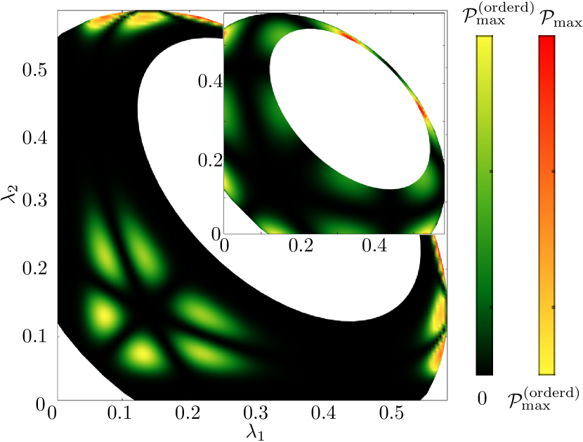
We can visualize the distribution for $n=4$ in figure 1. This distribution has a peak at $n-1$ degenerate states, modulated by a repulsion of levels, which, altogether creates a “cleaved peak”. Notice that at $m=n$ there is a qualitative change of behavior, and a repulsion from the planes $\lambda_{i}=0$ is not observed, since the term $\prod_{i}\lambda_{i}^{|m-n|}$ yields a constant. Level repulsion, however, is always present.

In order to gain some insight into the behavior of the eigenvalue distribution, and to make an approximation for large environments, let us first rewrite (6) as

$$\mathcal{P}=C_{m,P}Jg^{|m-n|}(\lambda)V(\lambda),$$

with $\lambda$ being the vector that groups all $\lambda_{i}$ and $C_{m,P}$ a normalization constant. The function

$$g(\lambda)=g(\lambda_{1,\dots,n-2},P)=\prod_{i=1}^{n}\lambda_{i}$$ (9)

is the product of all eigenvalues, but can be regarded as a function of the first $n-2$ eigenvalues and the purity. Finally,

$$V(\lambda)=V(\lambda_{1,\dots,n-2},P)=\prod_{i<j}(\lambda_{i}-\lambda_{j})^{2}$$ (10)

is a Vandermonde determinant. These two terms, $g$ and $V$, shall be analyzed separately. We will see that $g(\lambda)$ is responsible for a peak around a $n-1$ degenerate state, whereas the determinant is responsible for the nodes that appear modulating such peak.

The peak

We find explicitly that

$$g(\lambda)=\frac{s_{2}+\left(s_{1}\right)^{2}-2s_{1}+1-P}{2}\prod_{i=1}^{n-2}\lambda_{i}.$$ (11)

To obtain the extrema of the function, the partial derivatives are set to zero. Assuming $\lambda_{i}>0$ and rearranging, we obtain from the subtraction of the equations obtained from the partial derivative of $g(\lambda)$ with respect to $\lambda_{j}$ and $\lambda_{k}$:

$$(\lambda_{j}-\lambda_{k})\left(\lambda_{j}+\lambda_{k}+s_{1}-1\right)=0$$ (12)

and from the sum of all partial derivatives,

$$s_{2}+\left(s_{1}\right)^{2}+2\frac{1-n}{n}s_{1}+\frac{n-2}{n}(1-P)=0.$$ (13)

In general, these equations have an exponentially large number of solutions, not all of them physical, but a detailed analysis turns out to be cumbersome. We first focus on the particular case in which all $\lambda_{i}=\Lambda$, $i=1,\dots,n-2$, which clearly leads to a solution of all eqs. (12). From (13), and solving a simple quadratic equation, one obtains two solutions,

$$\Lambda_{\pm}=\frac{1}{n}\pm\frac{1}{n}\sqrt{\frac{nP-1}{n-1}}.$$ (14)

Each of this highly degenerate eigenvalues determines the other two eigenvalues, according to (7). These are $\lambda_{n-1}=\Lambda_{\pm}$ and $\lambda_{n}=1-(n-1)\Lambda_{\pm}$. This corresponds to a state that is a mixture of a pure state and the maximally mixed state. Notice that for $P>1/(n-1)$, $\Lambda_{+}$ results in a negative (and thus inadmissible) $\lambda_{n}$.

We can simplify the expression for the probability density near the maximum corresponding to the point $\lambda_{i}=\Lambda_{-}$, $i=1,\dots,n-1$. We expand in Taylor series around the maximum, and note that

$$\frac{\partial^{2}g}{\partial\lambda_{j}^{2}}{\biggr{|}}_{\lambda_{i}=\Lambda_{-}}=2\frac{\partial^{2}g}{\partial\lambda_{j}\lambda_{k\neq j}}{\biggr{|}}_{\lambda_{i}=\Lambda_{-}}=2\Lambda_{-}^{n-2}\left(n-\frac{1}{\Lambda_{-}}\right),$$ (15)

with $j=1,\dots,n-2$. This leads to

$$g(\lambda_{1,\dots,n-2},P)\approx g_{\text{max}}-\alpha\tilde{\lambda}\cdot A\cdot\tilde{\lambda}^{T}$$ (16)

with

$$A=\begin{pmatrix}2&1&\dots&1\\ 1&2&\dots&1\\ \vdots&\vdots&\ddots&\vdots\\ 1&1&\dots&2\end{pmatrix},$$

$\alpha=\Lambda_{-}^{n-2}\left(n-1/\Lambda_{-}\right)$, $\tilde{\lambda}=\begin{pmatrix}\lambda_{1}-\Lambda_{-}&\cdots&\lambda_{n-2}-\Lambda_{-}\end{pmatrix}$ and $g_{\text{max}}=g|_{\lambda_{i}=\Lambda_{-}}$. Recall that $\rme^{-x}\approx 1-x$ for small values of $x$, so that, near a maximum, one can approximate a polynomial with a Gaussian: $(1-x^{2})^{m}\approx\rme^{-mx^{2}}$ for $m\gg 1$ and $-1<x<1$. It is then found that

$$g(\lambda_{1,\dots,n-2},P)^{|m-n|}\approx g_{\text{max}}^{|m-n|}\exp\left(-\frac{\tilde{\lambda}^{T}\cdot A\cdot\tilde{\lambda}}{\sigma_{m,P}^{2}}\right)$$ (17)

with the average standard deviation given by with the factor $\sigma_{m,P}^{2}=g_{\text{max}}/\alpha(m-n)$ determining the standard deviation of each of the eigenvalues.

The Vandermonde determinant

We will study the situations in which $V(\lambda)=0$, as this will give information about the nodes of the probability density that will help understand its behavior. This happens when at least one of the terms $\lambda_{i}-\lambda_{j}=0$ ($i\neq j$). In the space of the first $n-2$ eigenvalues, the conditions

$$\lambda_{1}=\lambda_{2},\quad \lambda_{1}=\lambda_{3}, \dots,\quad \lambda_{1}=\lambda_{n-2}$$

$$\lambda_{2}=\lambda_{3}, \dots,\quad \lambda_{2}=\lambda_{n-2}$$

$$\ddots$$

$$\lambda_{n-3}=\lambda_{n-2}$$ (18)

are simple hyperplanes. On the other hand, replacing the conditions $\lambda_{j}=\lambda_{n-1}$ and $\lambda_{j}=\lambda_{n}$ on (7) and squaring the discriminant for $j=1,\dots,n-2$, define the $n-2$ different quadratic forms

$$Q_{j}(\lambda_{i})=\left(2\lambda_{j}+s_{1}-1\right)^{2}-2(P-s_{2})+(1-s_{1})^{2}=0.$$ (19)

All these curves are ellipsoids, as can be noted by the fact that all $\lambda$’s are bounded in these degree 2 polynomials. The condition $\lambda_{n-1}-\lambda_{n}=0$ can be calculated directly form (7), and leads to the ellipsoid

$$Q_{n}=2(P-s_{2})-(1-s_{1})^{2}=0,$$ (20)

which marks the limits for which the expression (7) lead to real, rather than complex and thus inadmissible, values for $\lambda_{n-1,n}$. Finally, the condition $\lambda_{n-1}=0$ constitutes another constraint, which can also be calculated from (7), and one obtains

$$Q_{n-1}=(P-s_{2})-(1-s_{1})^{2}=0.$$ (21)

Notice that the condition $\lambda_{n}=0$ is automatically taken care of, as from (7), $\lambda_{n}\geq\lambda_{n-1}$. The ellipsoids are really symmetry planes, that acquire this skew form since the last two eigenvalues are given a special status. One could focus the study to one region defined by any side of each of the ellipsoids (19).

At the peak, there is an $n-1$ fold degeneracy of the eigenvalues. The right hand side of (10) may be approximated, considering only linear terms with respect to $\lambda_{j}-\Lambda_{-}$. We obtain from the linear approximation $q_{j}(\lambda_{i})$ of $Q_{j}(\lambda_{i})$

$$q_{j}(\lambda_{i}) =(\lambda_{j}-\Lambda_{-})\frac{\partial Q_{j}}{\partial\lambda_{j}}{\biggr{|}}_{\lambda_{i}=\Lambda_{-}}+\sum_{k\neq j}(\lambda_{k}-\Lambda_{-})\frac{\partial Q_{j}}{\partial\lambda_{k}}{\biggr{|}}_{\lambda_{i}=\Lambda_{-}}$$

$$=4(n\Lambda_{-}-1)[\lambda_{j}+s_{1}-(n-1)\Lambda_{-}],$$ (22)

a series of $n-2$ hyperplanes. This approximation will be useful when combined with (17) to yield a simple expression near the degeneracy.

Figure 2: (Color online) Boundaries for the possible physical states, and visualization of the Vandermonde determinant in the $\lambda_{1}$, $\lambda_{2}$ plane, for $P=0.4$ and $n=4$. The regions where the physical density matrices live is above the horizontal [red] line ($\lambda_{2}\geq 0$), to the right of the vertical [red] line ($\lambda_{1}\geq 0$), inside the outer [green] ellipse [real values for $\lambda_{3}$ and $\lambda_{4}$, eqs. (20) and (24)] and outside the smaller [red] ellipse [$\lambda_{3}\geq 0$, eqs. (21) and (25)]. The geometric place of the $\lambda_{1}=\lambda_{2}$ degeneracy is the diagonal line [blue], of the $\lambda_{1}=\lambda_{3}$ and $\lambda_{1}=\lambda_{4}$ degeneracy is the most vertical [blue] ellipse and the $\lambda_{2}=\lambda_{3}$ and $\lambda_{2}=\lambda_{4}$ degeneracy is the most horizontal [blue] ellipse, see eqs. (19) and (23).

3.2 The special case of $n=4$

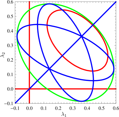
The case $n=4$ deserves special attention, as the numerics are carried on there, and a complete plot of the full distribution is possible. The explicit form of $g$ and $\Lambda_{-}$ can be read directly from eqs. (11) and (14). The analysis of the conditions of degeneracy results more interesting. In this case, the ellipsoid corresponding to $\lambda_{1}=\lambda_{3}$ and $\lambda_{1}=\lambda_{4}$ is

$$Q_{1}(\lambda_{1},\lambda_{2})=3\lambda_{1}^{2}+\lambda_{2}^{2}+2\lambda_{1}\lambda_{2}-2\lambda_{1}-\lambda_{2}+\frac{1-P}{2}.$$ (23)

This is an ellipse centered in $(1/4,1/4)$ rotated an angle $\theta$ such that $\cot\theta=1+\sqrt{2}$ and with semi-axes of length $\sqrt{4P-1}/4\sqrt{1\pm 2^{-1/2}}$. $Q_{2}$ will be the same up to an interchange of $\lambda_{1}$ and $\lambda_{2}$. The border curve corresponding to $\lambda_{3}=\lambda_{4}$ leads to the polynomial

$$Q_{4}(\lambda_{1},\lambda_{2})=3\lambda_{1}^{2}+3\lambda_{2}^{2}+2\lambda_{1}\lambda_{2}-2\lambda_{1}-2\lambda_{2}-2P+1.$$ (24)

This defines an ellipse with center in $(1/4,1/4)$, rotated by $\pi/4$ and with semiaxis $(\sqrt{4P-1}/3,\sqrt{(4P-1)/3})$.

Semi-definite positivity of the density operator is guarantied if one restricts to the area delimited by $\lambda_{i}\geq 0$, which amounts to consider the quadrant $\lambda_{1,2}\geq 0$, and $\lambda_{3}\geq 0$ as, by construction, $\lambda_{4}\geq\lambda_{3}$. The condition $\lambda_{3}\geq 0$ is met in the exterior of the ellipsoid defined by $Q_{3}(\lambda_{1},\lambda_{2})=0$ with

$$Q_{3}(x,y)=2x^{2}+2y^{2}+2xy-2x-2y+1-P.$$ (25)

This is an ellipsoid centered in $(1/3,1/3)$, rotated $\pi/4$ and with semiaxis $(\sqrt{3P-1}/3,\sqrt{(3P-1)/3})$. For $P<1/3$ this ellipse does not exist; as long as the previous conditions are met, $\lambda_{4}$ will be real.

Using approximation (22) the following simplified distribution is obtained

$$\mathcal{P}(\lambda_{1},\lambda_{2})=C_{P}\exp\left[-\frac{\tilde{\lambda}^{T}\cdot A\cdot\tilde{\lambda}}{\sigma_{m,P}^{2}}\right]\left[(\lambda_{1}-\lambda_{2})(2\lambda_{1}+\lambda_{2}-3\Lambda_{-})(\lambda_{1}+2\lambda_{2}-3\Lambda_{-})\right]^{2},$$ (26)

valid for large dimensions of the environment and sufficiently close to $\lambda_{1,2,3}\approx\Lambda_{-}$. It is now simple to read the behavior of the function. It is indeed a 6-fold peaked function arising from a Gaussian of width diminishing as $1/\sqrt{m}$, modulated by some parabolas touching zero. In this approximation the center of the Gaussian is located in the point $\vec{\Lambda}_{-}=(\Lambda_{-},\Lambda_{-})$ with $\Lambda_{-}=(3-\sqrt{12P-3})/12$; a point corresponding to a triply degenerate state. The other peaks are in $\vec{\Lambda}_{-}+\sigma_{m,P}\vec{v}_{i}$ where $\vec{v}_{1,\ldots,6}\in\{(\pm\sqrt{3},0),(0,\pm\sqrt{3},0),\sqrt{2}(\pm 1,\mp 1)\}$. The last thing that should be calculated are single variable distributions, which are presented in appendix B.

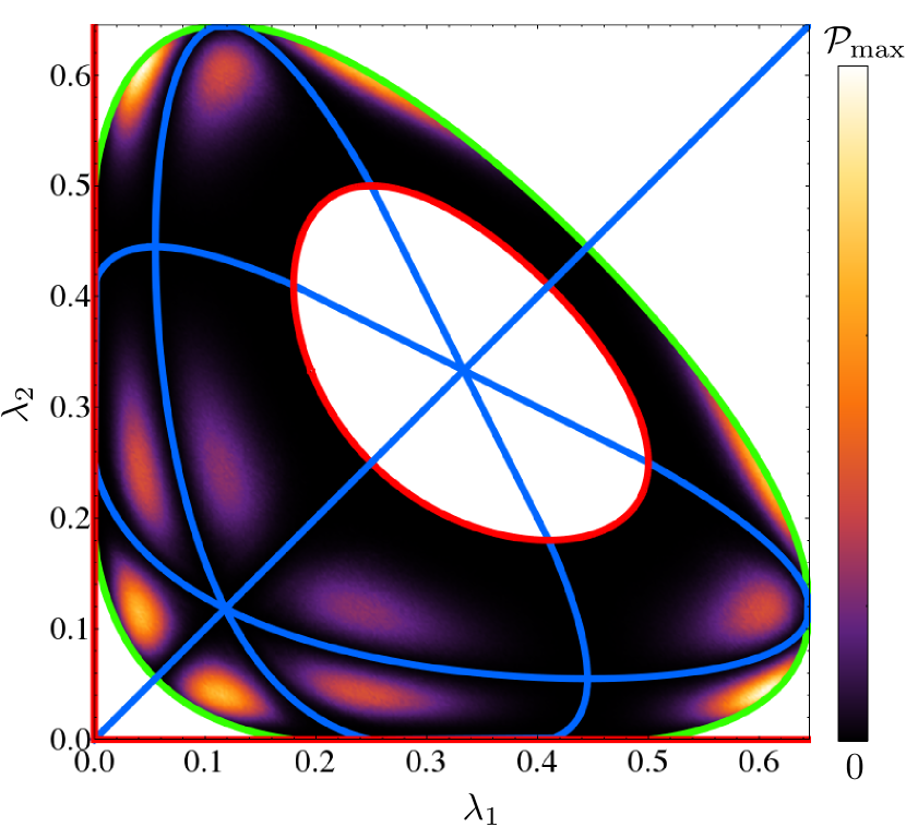
A glimpse at the complexity of the surface can be obtain analyzing the stationary points of the surface. In this case, (12) and (13) lead to four solutions. The first one corresponds to $\lambda_{1}=\lambda_{2}=\Lambda_{-}$. The other two eigenvalues are $\Lambda_{-}$ and $1-3\Lambda_{-}$. A second solution, corresponding to triply degenerate $\Lambda_{+}$ remains physical for $P\leq 1/2$, after which the points migrate to the unphysical region corresponding to the interior of the red ellipse in figure 2. The other two solutions correspond to saddle points of the function $g$, but for $P>1/2$ also correspond to unphysical eigenvalues. There are additional maximums that are not detected by conditions (12) and (13), which live in the edge of the domain, and thus would have to be calculated separately. These also correspond to the same triply degenerate states with $\Lambda_{-}$, but reordered and are located at the points in which the blue and green ellipses in figure 2 touch each other.

All these boundaries are plotted in figure 2, where one can visualize the roll of each of the conditions earlier discussed. The global effect can also be nicely seen in figure 1.

4 Random states and random dynamics

We now wish to compare the results obtained for the static model discussed in the previous section with those of previously studied dynamical random matrix models, in which decoherence of a central system can be studied [32, 5, 12]. These models are time independent, but will be used to evolve an initial state until a time in which the purity (or any other quantity of interest) reaches the particular value of interest, thus obtaining an equivalent ensemble of density matrices.

That said, consider again a Hilbert space with the structure ${\mathcal{H}}\ =\ \mathcal{H}_{\textrm{cen }}\otimes\mathcal{H}_{\textrm{env}}$ [recall (2)]. As in sec. 3.2, we also restrict to the case in which $\mathcal{H}_{\textrm{cen }}$ is a 4-level system. Special consideration will be given to the case in which $\mathcal{H}_{\textrm{cen }}$ is composed of two qubits; that is, when

$$\mathcal{H}_{\textrm{cen }}={\mathcal{H}}_{{\textrm{q}}_{1}}\otimes{\mathcal{H}}_{{\textrm{q}}_{2}}.$$ (27)

where ${\mathcal{H}}_{{\textrm{q}}_{i}}$ denote qubit spaces. In this space, unitary dynamics will be generated by random Hamiltonians, to be detailed later. Non-unitary dynamics in the two qubit central system is thus induced by the unitary dynamics in the whole space, plus partial tracing over $\mathcal{H}_{\textrm{cen }}$. As initial states, pure separable states in the whole Hilbert space are used:

$$|\psi(0)\rangle=|\psi_{\textrm{cen }}\rangle|\psi_{\textrm{env}}\rangle,\quad|\psi_{\textrm{cen }}\rangle\in\mathcal{H}_{\textrm{cen }},\,|\psi_{\textrm{env}}\rangle\in\mathcal{H}_{\textrm{env}};.$$ (28)

We take $|\psi_{\textrm{env}}\rangle$ to be a random state, according to the Haar measure of the unitary group in the environment, but $|\psi_{\textrm{cen }}\rangle$ is to be chosen according to the particular case under study.

Kolmogorov distance will be used to quantify the difference between two distributions. Given two functions, $f(x)$ and $g(x)$, defined on a domain $X$, it is

$$K(f,g)=\frac{1}{2}\int_{X}|f(x)-g(x)|\rmd x.$$ (29)

Notice that since we are dealing with distributions, the normalization condition for a distribution $\mathcal{P}(x)$ is stated as $K(\mathcal{P},0)=\frac{1}{2}$, and thus the distance between two non overlapping (i.e. totally distinct) distributions $\mathcal{P}_{1}$ and $\mathcal{P}_{2}$ is always 1.

4.1 Global Hamiltonian

Figure 3: (Color online) Marginal distribution of the smallest two eigenvalues ($\lambda_{1}\leq\lambda_{2}$). The points are obtained with nonunitary evolution under the global Hamiltonian (30) with close to $10^{6}$ realizations, and the curves are obtained with the marginal distributions (44) and (49), obtained by proper integration of (6). We show different target purities and different environment dimensions.

The simplest candidate for a random matrix model that describes decoherence is simply choosing a Hamiltonian from one of the classical ensembles [17] that acts on the whole Hilbert space, i.e. on both the central system and the environment [5]. We shall call this family global Hamiltonian. These Hamiltonians are attractive because of their analytic simplicity [12]. They also model the strongest interaction between central system and environment. We shall choose to pick the Hamiltonian from the GUE (Gaussian unitary ensemble) as it is the simplest ensemble, from an analytical point of view.

For this case, we can write simply

$$H=H^{(\text{GUE})}_{{\textrm{env}},{\textrm{cen }}}$$ (30)

where the superindex indicates the ensemble from which the operator is chosen, and the subindices indicate the spaces in which they act non-trivially. For this case, and due to the invariance of the GUE, one can choose the initial state of the central system arbitrarily, with no effect on the results regarding the eigenvalue density of the evolved state of the central system.

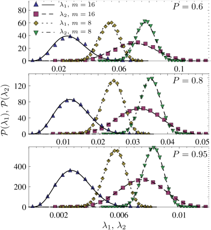
The eigenvalue density of the density matrices produced by the non-unitary dynamics induced by the Hamiltonian (30) are similar to those for the static situation, (6). However, differences can be observed by inspection, see figure 3. These differences are larger for smaller purities, and seem to be independent of the size of the environment. However, even for an intermediate purity of $P=0.8$, it is difficult to see any differences. If one is not interested in very precise data, or only in high purity, quantitative information can be extracted from the static model regarding the evolved state.

Figure 4: Marginal distribution of the smallest eigenvalue $\lambda_{1}$. The points are obtained with nonunitary evolution under the tunable coupling Hamiltonian (31) with close to $10^{5}$ realizations, and the curves are obtained with the marginal distributions (44) and (49), obtained by proper integration of (6). We show two different target purities, different environment dimensions and different couplings. For very small couplings, the ensemble is not well approximated by (6), but already for moderate couplings, the ansatz is very good.

4.2 Tunable coupling

Hamiltonian (30) couples the central system and its environment. However it does not take into account the structure of Hilbert space (2). One way to do that is to provide the Hamiltonian governing the system with a similar tensor product structure. Moreover this will lead the idea of tunable coupling which is very convenient when studying open quantum systems. We thus use

$$H=H^{(\text{GUE})}_{{\textrm{env}}}+\epsilon V^{(\text{GUE})}_{{\textrm{env}},{\textrm{cen }}},$$ (31)

which will be called tunable coupling Hamiltonian, or coupling Hamiltonian, for short. It must be noticed that the case $\epsilon\to\infty$ corresponds, up to a rescaling in time, to the previous case, i.e. (30).

Regarding the eigenvalue density of the evolved state of the central system with Hamiltonian (31), a significant dependency on the coupling strength was observed. Four regimes should be considered: weak coupling [for which $\epsilon=0.01$ is taken as a representantive], intermediate coupling [$\epsilon=0.1$], strong coupling [$\epsilon=1$], and very strong coupling [$\epsilon\to\infty$].

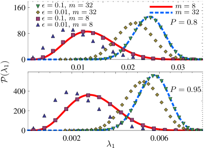
For weak coupling there is a clear discrepancy, for all purities and dimensions examined. The agreement does not seem to improve for larger dimensions, see figure 4. It must be noticed that even though there is a significant disagreement between the two ensembles, the nodes can still be observed, and for a qualitative description, the static ensemble is still useful.

For intermediate coupling $\epsilon=0.1$, the agreement is very good, and only for smaller dimensions and purities can the difference be observed by inspection, see figure 4. Here, it seems that both, increasing the purity at fixed environment dimension, and increasing the dimension at fixed purity leads to the same ensemble as the static one. For strong coupling and very strong coupling, the results are indistinguishable from the global Hamiltonian case, see figure 6.

4.3 Spectator Hamiltonian

An interesting variation of (31) has been studied in [13]. There, one studies a central system whose Hilbert space is composed of two qubits. That is when the Hilbert space is of the form (27). There, the spectator Hamiltonian

$$H=H^{(\text{GUE})}_{\textrm{env}}+\epsilon V^{(\text{GUE})}_{{\textrm{env}},{\textrm{q}}_{1}}$$ (32)

was proposed where, again, the subindices indicate the part of the Hilbert space where they act non trivially. The first term correspond to the free dynamics of the environment. The next represents the coupling of the first qubit to the environment. Thus, the second qubit is simply a spectator, as it has no coupling to an environment. This is the simplest Hamiltonian for which we can analyze the effect of an environment on a Bell pair [13]. The environment Hamiltonian $H_{\textrm{env}}$ will be chosen from a classical ensemble [17] of $m\times m$ matrices and the coupling $V_{{\textrm{env}},{\textrm{q}}_{1}}$ from one of $2m\times 2m$ matrices.

Figure 5: Distribution of the two smallest eigenvalues for the spectator and the common environment Hamiltonians eqs. (32), (35), for various degrees of entanglement of the initial condition in the central system, modulated by $\theta$ in (34). The target purity is, in this case, $P=0.8$ and we fix $m=8$. For the spectator case, low entanglement tends to push the distribution towards the origin, and for the common environment, small entanglement tends to push the distribution towards the $y$ axis. Both models are in good agreement with the ansatz distribution for a maximally entangled initial state. The figure shows a disymmetrized distribution, assuming non-decreasing eigenvalues, and the scale is arbitrary.

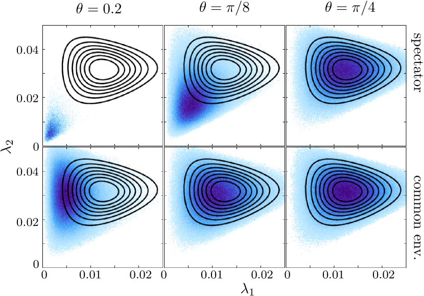
This Hamiltonian is quite interesting, since it does not involve one of the qubits. At least not from the dynamical point of view. This Hamiltonian adds a structure to the problem: it creates the notion of a particle. One obvious new ingredient when the Hilbert space is split is entanglement. In this case we shall thus have a new parameter which is the entanglement of the initial state in the two qubits.

Figure 6: We present a summary of the comparison between the static ensemble, and the ensemble generated by random dynamics (left). In the ordinate $\log_{2}m$ with only take integer values. The symbols representing the different cases will appear for arbitrary values within the interval around the fixed integer value of $\log_{2}m$ to make then discernible. On the abscissa the Kolmogorov distance between the dynamical model and the corresponding static one $K(\mathcal{P},\cdot)$ is plotted. Good agreement between both is observed for the global Hamiltonian, the coupling Hamiltonian for large enough coupling, and for the spectator and common environment Hamiltonian when the initial state has maximal entanglement. The symbols must be understood using the table on the right hand side. The error bars are obtained with the Kolmogorov distance with respect to a Monte Carlo simulation with the same number of points as the one with the random dynamics, that is, $10^{6}$ points.

For a totally disentangled initial state, the dynamics will produce in the two qubits a reduced state of the form

$$\rho(t)=\rho_{1}(t)\otimes|\psi\rangle\langle\psi|$$ (33)

at all times. Notice that the smaller eigenvalues $0$ are double degenerate. The other two eigenvalues are totally determined by the normalization condition and the fixed purity condition.

Taking into account the invariance of the ensemble defined by (32) under local unitary operations, we notice that the initial states can be written with absolute generality as

$$|\psi(0)\rangle=\sin\theta|00\rangle+\cos\theta|11\rangle,\quad\rho(0)=|\psi(0)\rangle\langle\psi(0)|,$$ (34)

where $\theta$ is the only relevant parameter of the state, and also modulates the initial entanglement. $\theta=0$ corresponds to an initially separable state, whereas $\theta=\pi/4$ to a maximally entangled one. If $\theta=0.2$ the situation is indeed close to the totally separable case. In this case the distribution is totally different than expected from the static analysis, that is from (6), see figure 5. However for a maximally entangled state $\theta=\pi/4$, the results are similar as to the tunable coupling case with four levels. That is, acceptable agreement for very small coupling, and much better agreement for intermediate coupling. Again, the agreement improves with increasing purity, but does not seems to converge for increasing dimension of the environment at a fixed purity, see figure 6.

4.4 Common environment Hamiltonian

Even though Hamiltonian (32) is the simplest one that allows us to study entanglement evolution [13], in many situations one would have coupling of all constituents of the central system to the environment. To be closer to many experimental situations, consider what we call the common environment Hamiltonian

$$H=H^{(\text{GUE})}_{\textrm{env}}+\epsilon V^{(\text{GUE})}_{{\textrm{env}},{\textrm{q}}_{1}}+\epsilon V^{(\text{GUE})}_{{\textrm{env}},{\textrm{q}}_{2}}.$$ (35)

Again, the indices indicate the subspaces in which they operate non-trivially, with respect to (2) and (27). This Hamiltonian, includes coupling of both qubits to an environment, but also takes into account a Hilbert space with the structure (27).

For the common environment Hamiltonian we have again a particular form of the eigenvalues for an initially separable state. In this case, one can approximate the dynamics as two channels acting independently on the two qubits. Thus, neglecting correlations in the environment, for later times one should have that

$$\rho(t)\approx\rho_{1}(t)\otimes\rho_{2}(t).$$ (36)

One then has that the eigenvalues of the reduced density matrix are $(\lambda,1-\lambda)\otimes(\lambda^{\prime},1-\lambda^{\prime})$, which gives an additional global restriction; the manifold in which the eigenvalues lives has dimension one, instead of two as in the previous cases. This will of course heavily influence the distributions of eigenvalues. For a small amount of initial entanglement the situation should vary continuously, and one indeed observes very significant differences with the proposed ansatz, see figure 6. For an initially maximally entangled state, the results are again similar and are well reproduced by the static ansatz, see figs. (5) and (6).

4.5 A comparison using Kolmogorov distance

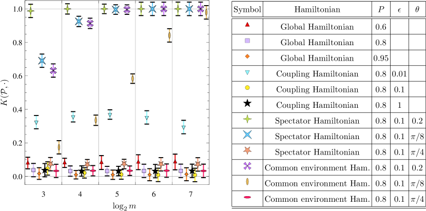
The results of this section can be summarized in a figure containing the Kolmogorov distance between the results for the dynamical system, and the statical ensemble, (6). We present those results in figure 6.

Error bars, obtained using the Kolmogorov distance between the exact distribution, and an equivalent Monte Carlo simulation [see Appendix C] with the same number of data points as the dynamical situation, is also included. This number should be interpreted as the error arising both from finite sampling and finite binning.

We can see that the results for the static model and the dynamical models agree well for the global Hamiltonian, and for the coupling Hamiltonian, as long as the coupling is not too small. If the coupling is very small, there are quantitative deviations, but the shape of the distribution remains similar. In this case, one can see that there is a clear difference between the static and the dynamical ensemble, which leads to intermediate values of $K$, very different both from 0 and 1. As coupling becomes very small, these deviations increase. Often such cases are associated with situations where the dynamical model will actually not reach equipartition [33, 11].

For models in which structured coupling is present (spectator and common environment models), one has similar results as for the tunable coupling model as long as the initial entanglement is maximal. For other initial states the disagreement is progressive as the dimension of the environment increases. We conjecture that in the limit of large $m$ there will be a dynamical quantum phase transition between good agreement and maximum disagreement, for arbitrarily small deviations from a Bell state.

5 Other functions: von Neumann entropy

Figure 7: (Color online) Probability distribution of the entropy $S$ for several values of purity. Each plot shows a particular purity and several dimensions of the environment. Notice the scale in the horizontal axis to observe that the distributions are already quite peaked for the dimensions shown, the effect being larger for increasing dimension.

We have also studied the von Neumann entropy (henceforth called entropy) of the reduced density matrix

$$S(\rho)=-\tr\left(\rho\ln\rho\right).$$ (37)

The algebraic structure is considerably more complicated than for purity, and thus such a detailed program as was presented in the previous sections is in general only possible in terms of solutions of transcendental equations. However much can be said using the fact that purity and entropy are closely related in typical cases.

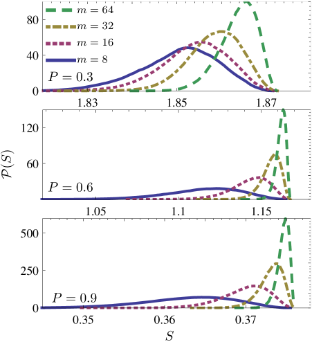
For the ensembles studied in section 3, consider the entropy. Its distribution is plotted in figure 7, for several fixed purities, and several dimensions of the environment. One can see that even for small dimensions of the environment ($m=8$), the width of the entropy distribution is already of order $10^{-2}$, and its value decreases with increasing $m$. Thus, even though the ensembles for fixed purity and fixed entropy are different (not even the support is the same), they are similar.

As an example, the equivalent to figures 1 and 2, but for fixed entropy, is shown in figure 8. We obtained numerically the corresponding limiting curves and nodes, and the probability distribution corresponding to the static ensemble. The resemblance to the case of purity is striking, and one may conclude that many of the results obtained for a fixed value of purity must hold qualitatively for a fixed value of the entropy.

Notice that we are considering just two functions of infinitely many that define a partial order over the eigenvalue vector, which mathematically corresponds to a probability distribution. This indicates that the entire theory developed by Hardy, Littlewood, and Polya [34] applies, as noted in reference [35, 36, 37]. In particular it indicates that the ordering becomes unique both near the pure states and near the maximally mixed state, thus formalizing the analogy between purity and, say, entropy when one approaches any of these limits.

Figure 8: (Color online) Probability distribution of 2 eigenvalues at fixed entropy $S=1.5$ for $m=8$, in arbitrary units. The white region leads to nonphysical eigenvalues. Nodes and limiting curves are also present here. The color coding is exactly the same as in figures 1 and 2.

6 Conclusions

In this paper we set out to give a random matrix model for density matrices of open quantum system by imposing further restrictions on an ensemble originally obtained by simply restricting an ensemble of random covariance matrices to matrices with unit trace. In section two we give some general remarks about the alternate possibilities of restricting random matrix ensembles in analogy to techniques used in statistical mechanics, as well as on the alternative of a proposing a random matrix description directly for the object of interest, as compared to proposing a random set of Hamiltonians to describe the dynamics and from that calculate the ensemble of that same object. In the latter case the condition is imposed by following evolution until it is fulfilled exactly (i.e. up to numerical exactitude).

The conditions can either be imposed in a “strict way” for each member of the ensemble resulting in microcanonical ensembles or on average in the spirit of Jayne’s principle leading to canonical ensembles. In view of the original construction [8] we opt for the microcanonical approach.

After the construction of the ensemble we concentrate on the distribution of eigenvalues of the density matrices using fixed purity as the additional restriction. The choice of purity allows us to obtain analytical results but we also consider alternate convex functions and explicitly the von Neumann entropy towards the end of the paper. Qualitatively very similar rests are obtained

To visualize our result we restrict our considerations to a four dimensional central system. The two restrictions imposed allow to give density maps over the two remaining dimensions and one clearly sees the signature of the Jacobi determinants on an otherwise smooth distribution limited by the boundaries imposed by the restrictions on trace and purity. Again, this picture remains qualitatively unchanged if we replace purity by von Neumann entropy.

For this four dimensional central system we present the comparison with the results obtained if we run the time evolution of an initially pure state of the central system under the random matrix model for decoherence given in terms of several families of random Hamiltonians for the full system (central system + environment). We find fairly good agreement if the fouling between environment and the central system is not too weak, i.e. if we are not in the “perturbative regime”. Surprisingly this holds true even if the four dimensional central system consists of two quits but one of the two does not interact with either the other or the environment, under the condition that the two qubits are maximally entangled.

We may speculate as to why the static and dynamic models agree so well, except for the case of partially entangled central systems with a structured coupling to the environment. Consider POSETS (partially ordered sets or lattices) of density matrices introduced by Uhlmann [37] as well as by Ruch and Mead [35, 36] independently. This work is based on a partial order introduced by Muirhead [38] and connected to classical bi-stochastic evolution by Hardy, Littlewood and Polya [34] (see also [35]). The classical evolution can be generalized to POSETS of pairs of distribution [39, 40] and such concepts seem to have a growing impact on recent work using majorization in the context of open quantum systems (e.g [41, 42, 43, 44]).

In this context it is well known, that near distributions with a dominant component (i.e. for almost pure states) all convex functions will yield essentially the same order, or, with other words, near its extreme points POSETS are almost completely ordered sets. Therefore a unitary dynamic acting on a initially separable density matrix will have no choice but to follow closely the time-independent partial order, which governs the static ensemble. Indeed if we look at figure 3 we see immediately that the agreement is best near maximal purity.

A number of steps along these lines are possible for the future. One may investigate if a partial orders for pairs, as suggested above, can be extended to pairs of density matrices. is feasible and weather it it brings any advantages. A note of caution must be added here, as the partial order for pairs of distributions in [39, 40] has not been successfully generalized to density matrices because the two members of the pair typically cannot be diagonalized with the same transformation. If and when this mathematical problem is overcome we may well find this to be the key to a deeper understanding of our results. Another more obvious next step is to calculate other quantities for fixed decoherence as measured by purity or some other convex function. For the two qubit case concurrence would be the obvious candidate, as it would allow to calculate $CP$ diagrams (concurrence purity) without referring to time evolution.

References

Appendix A A isometrical description for the 2 qubit case

Figure 9: (Color online) Region of interest. The boundary between positive (physical) eigenvalues and negative is showed in red, for each of the eigenvalues. The border between some degenerate eigenvalues is plotted in blue. Thus, the physical region with sorted eigenvalues restricts only to the black area.

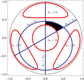
For the 2 qubit case, one case visualize the distribution of eigenvalues in the $(\lambda_{1},\lambda_{2})$ plane. However this is not the only way of visualizing the results. One would like a way that preserves the natural symmetry of the problem, and that conserves a notion of “volume” in this space. Taking the natural volume in $\Re^{n}$, one can come up with an isometry, after rotating, doing an isometrical stereographical projection, a simple plane. There, one can calculate the position of triple degenerate states, and the physical regions ($\lambda_{i}>0$).

One reason to perform the analysis done with the other visualization, is that reading the eigenvalues directly from a point in the plane is straightforward. With the representation presented in this appendix, it is not the case. One thus sacrifices symmetry and isometry for clarity.

We shall initially restrict to the 3 dimensional space defined by the normalization condition. We found convenient to transform condition 3 to one that involves a single variable. A rotation seems the most appropriate, and since the distance to the origin must remain invariant, one has to search for a rotation that transforms 3 to

$$\lambda_{1}=1/2.$$ (38)

This is the same rotation that transforms the vector $(1/2,1/2,1/2,1/2)$ (normal to the hyperplane 3) to the vector $(1,0,0,0)$ (normal to the hyperplane 38). One can build such a rotation with a sequence of 2-dimensional rotations, the first acting on the last two coordinates and transforming $(1/2,1/2)$ to $(\sqrt{2}/2,0)$, the second one acting on the second and third coordinate and transforming thus $(1/2,\sqrt{2}/2)$ to $(\sqrt{3}/2,0)$ and the last one acting on the first two coordinates and taking $(1/2,\sqrt{3}/2)$ to $(1,0)$. The overall sequence of rotations lead to the matrix

$$R=\begin{pmatrix}\frac{1}{\sqrt{2}}&-\frac{1}{\sqrt{2}}&0&0\\ \frac{1}{\sqrt{6}}&\frac{1}{\sqrt{6}}&-\frac{\sqrt{6}}{3}&0\\ \frac{1}{2\sqrt{3}}&\frac{1}{2\sqrt{3}}&\frac{1}{2\sqrt{3}}&-\frac{\sqrt{3}}{2}\\ 1/2&1/2&1/2&1/2\end{pmatrix}.$$ (39)

The condition regarding purity transforms trivially: a rotated hyper-sphere is a hyper-sphere. The intersection of the “rotated” sphere with the rotated hyperplane (38) can be readily evaluated, and yields

$$\sum_{i=2}^{4}\lambda_{i}^{2}=P-\frac{1}{4}$$ (40)

which is the familiar 3-sphere with a radius ranging from 0 to $3/4$.

The planes which describe the semi positivity condition of the eigenvalues are transformed into planes in $\mathbb{R}^{3}$ with equations

$$2\sqrt{3}\lambda_{4} \leq 1$$ (41a)

$$2\sqrt{2}\lambda_{3}-\lambda_{4} \leq\frac{\sqrt{3}}{2}$$ (41b)

$$\sqrt{6}\lambda_{2}-\sqrt{2}\lambda_{3}-\lambda_{4} \leq\frac{\sqrt{3}}{2}$$ (41c)

$$-\sqrt{6}\lambda_{2}-\sqrt{2}\lambda_{3}-\lambda_{4} \leq\frac{\sqrt{3}}{2}$$ (41d)

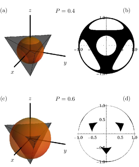
These planes define a regular tetrahedron, inside which must lay the (rotated) eigenvalues of any physical density matrix. For $P<1/3$ the sphere is completely inside the tetrahedron, and at $P=1/3$ it is tangent to the faces. At $P=1/2$ the sphere touches the vertexes. Finally, at $P=1$ it touches the tetrahedron only in the corners, allowing only 4 situations, namely when a single eigenvalue is 1 and the others are 0. We invite the reader to refer to Figs. 10, (a) and (c).

The next step is to project the sphere obtained to a plane, but keeping the natural measure in $\mathbb{R}^{n}$. Thus the usual stereographic projection is not an option. We write the point in the three dimensional space, previously found, in spherical coordinates $(r,\theta,\phi)$, and map them to polar coordinates in the plane $(R,\vartheta)$. As for a fixed purity one has constant $r$, this coordinate can be ignored. Mapping $\phi\to\vartheta$ and choosing $R$ as a function (to be determined) of $\theta$ so as to make an “stretched” stereographic projection, will do the required job. With that freedom one can make the transformation an isometry. The isometry requirement can be written formally as

$$\sin\theta\rmd\theta\propto R\rmd R$$ (42)

ignoring a normalization constant. This can be fulfilled using $R=\sin(\theta/2)$.

In figure 9, we present the limiting regions studied before. That is, the regions which delimit the semi-positive definitiveness of the density matrix. That is, where the eigenvalues are zero. This results in four red curves, with a threefold symmetry. Moreover, the curves that represent the degenerate points ($\lambda_{i}=\lambda_{j}$) necessary to delimit the region that leads to ordered eigenvalues are presented in blue. That region is colored in black.

We are now interested in the allowed areas [black regions in figure 10 (b) and (d)]. However an analytic form of the curve seems to be too complicated to be obtained. One can still appreciate a high degree of symmetry in the plot. This is due to the possibility of exchanging different eigenvalues. This brings up 24 equivalent zones, since there are $4!=24$ ways of ordering 4 different objects. Since the ordering will not bring any difference in the distributions, one can restrict to the area in which

$$\lambda_{i}\geq\lambda_{i+1}.$$ (43)

Figure 10: (Color online) Representation of the eigenvalues in the hyperplane where the normalization condition is met (left) and its projection to two dimensions using a measure preserving map. We show two values of purity ($P=0.4,0.6$ for the top/bottom figure) where the region is connected and disconnected.

Appendix B Distribution of individual eigenvalues

One can consider the individual distributions of the ordered eigenvalues. We can study such distribution in the $(\lambda_{1},\lambda_{2})$ plane. We shall then restrict to the area that contains $\lambda_{i}\geq\lambda_{i+1}$ indicated by a dark curve enclosing the area of interest in figure 2. To obtain the distribution of the smallest eigenvalue, the following integral must be performed:

$$\mathcal{P}_{\lambda_{1}}(\lambda_{1,\min}\leq\lambda_{1}\leq\lambda_{1,\max})\\ \propto\int_{\lambda_{2,\min}(\lambda_{1})}^{\lambda_{2,\max}(\lambda_{1})}\rmd\lambda_{2}\prod_{i}\lambda_{i}^{m-4}\prod_{i<j}(\lambda_{i}-\lambda_{j})^{2}$$ (44)

with $\lambda_{3,4}=\lambda_{3,4}(\lambda_{1},\lambda_{2})$ given by (14) and the limits being given by the relations

$$\lambda_{1,\min} =\max\left\{0,\frac{1}{4}\left(1-\sqrt{12P-3}\right)\right\}$$ (45)

$$\lambda_{1,\max} =\frac{3-\sqrt{12P-3}}{12}$$ (46)

$$\lambda_{2,\min}(\lambda_{1}) =\max\left\{\lambda_{1},\frac{1-\lambda_{1}-\sqrt{6P-2+4\lambda_{1}-8\lambda_{1}^{2}}}{3}\right\}$$ (47)

$$\lambda_{2,\max}(\lambda_{1}) =\frac{2-2\lambda_{1}-\sqrt{6P-2+4\lambda_{1}-8\lambda_{1}^{2}}}{6}.$$ (48)

Similarly one can obtain the distribution for the second smallest eigenvalue:

$$\mathcal{P}_{\lambda_{2}}(\lambda_{2,\min}\leq\lambda_{2}\leq\lambda_{2,\max})\\ \propto\int_{\lambda_{1,\min}(\lambda_{2})}^{\lambda_{1,\max}(\lambda_{2})}\rmd\lambda_{1}\prod_{i}\lambda_{i}^{m-4}\prod_{i<j}(\lambda_{i}-\lambda_{j})^{2}$$ (49)

with

$$\lambda_{2,\min} =\max\left\{0,\frac{1}{4}\left(1-\sqrt{4P-1}\right)\right\}$$ (50)

$$\lambda_{2,\max} =\begin{cases}\frac{2-\sqrt{6P-2}}{6}&\text{$P>1/3$},\\ \frac{3-\sqrt{12P-3}}{12}&\text{$P\leq 1/3$}\end{cases}$$ (51)

$$\lambda_{1,\min}(\lambda_{2}) =\max\left\{0,\frac{1-\lambda_{2}-\sqrt{6P-2+4\lambda_{2}-8\lambda_{2}^{2}}}{3}\right\}$$ (52)

$$\lambda_{1,\max}(\lambda_{2}) =\min\left\{\lambda_{2},\frac{1-2\lambda_{2}-\sqrt{2P-1+4\lambda_{2}-8\lambda_{2}^{2}}}{2}\right\}.$$ (53)

The expressions for the projected probabilities are straightforward to obtain for fixed $m$, but in general result in lengthy expressions, that can be obtained from a computer program.

Appendix C Monte Carlo simulations

We performed Monte Carlo simulations of the eigenvalues at fixed purity and entropy. This was done for the following three reasons. (i) To check the formulae obtained; (ii) to estimate the statistical error in calculating the Kolmogorov distance, due both to finite sampling and finite binning; and (iii) to calculate the distribution of the eigenvalues at fixed entropy, as it is easier than solving the resulting transcendental equation. Inspired in [8], we consider a potential energy for the eigenvalues of

$$E(\vec{\lambda})=-(m-4)\sum_{i}\log\lambda_{i}-2\sum_{i<j}\log|\lambda_{i}-\lambda_{j}|$$ (54)

for $\lambda_{i}\in\mathbb{R}^{+}$. A step in which the first two eigenvalues are displaced in a random angle a distance $\epsilon$ is used, and the other two are obtained by requiring normalization and the desired value of purity. That way, fixed purity and normalization condition are ensured. Moreover, if this results in a negative eigenvalue, its absolute value is taken. With these conditions, $\epsilon$ is set such that the acceptance rate is between $0.4$ and $0.6$. The particular value depends strongly on both $m$ and $P$. To perform the simulations for fixed entropy, one can simply solve for the other two eigenvalues, but, of course, at fixed entropy. This is however considerably more demanding. This method can be generalized for arbitrary dimensions, one should just perform a random walk in $n-2$ dimensions, with potential energy given by eq. (54), and calculate the other two eigenvalues to fulfill the conditions of normalization and fixed, say, purity.

References

- [1] J. von Neumann. Mathematical Foundations of Quantum Mechanics. Princeton University Press, 1955.
- [2] H.P. Breuer and F. Petruccione. The Theory of Open Quantum Systems. OUP Oxford, 2007.
- [3] G. Lindblad. On the generators of quantum dynamical semigroups. Communications in Mathematical Physics, 48(2):119–130, June 1976.
- [4] Vittorio Gorini, Andrzej Kossakowski, and E C G Sudarshan. Completely positive dynamical semigroups of N-level systems. Journal of Mathematical Physics, 17(5):821, May 1976.
- [5] T. Gorin and T. H. Seligman. Decoherence in chaotic and integrable systems: a random matrix approach. Phys. Lett. A, 309:61–67, Mar 2003.
- [6] T. Gorin, C. Pineda, H. Kohler, and T. H. Seligman. A random matrix theory of decoherence. New J. Phys., 10(11):115016–+, November 2008.
- [7] C. Nadal, S. N. Majumdar, and M. Vergassola. Phase transitions in the distribution of bipartite entanglement of a random pure state. Phys. Rev. Lett., 104(11):110501, Mar 2010.
- [8] Celine Nadal, Satya N. Majumdar, and Massimo Vergassola. Statistical Distribution of Quantum Entanglement for a Random Bipartite State. Journal of Statistical Physics, 142(2):403–438, January 2011.
- [9] P. A. Mello, P. Pereyra, and T. H. Seligman. Information theory and statistical nuclear reactions. i. general theory and applications to few-channel problems. Annals of Physics, 161(2):254 – 275, 1985.
- [10] F. Haake. Quantum Signatures of Chaos, II ed. Springer, Berlin, 2001.
- [11] C. Pineda, T. Gorin, and T. H. Seligman. Decoherence of two-qubit systems: a random matrix description. New J. Phys., 9(4):106, April 2007.
- [12] M. Žnidarič, C. Pineda, and I. García-Mata. Non-markovian behavior of small and large complex quantum systems. Phys. Rev. Lett., 107(8):080404, Aug 2011.
- [13] C. Pineda and T. H. Seligman. Bell pair in a generic random matrix environment. Phys. Rev. A, 75(1):012106, 2007.
- [14] D Agassi, H.A Weidenmüller, and G Mantzouranis. The statistical theory of nuclear reactions for strongly overlapping resonances as a theory of transport phenomena. Physics Reports, 22(3):145 – 179, 1975.
- [15] J. J. M. Verbaarschot, H. A Weidenmüller, and M. R. Zirnbauer. Grassmann integration in stochastic quantum physics: the case of compound-nucleus scattering. Phys. Rev., 129(6):367–438, 1985.
- [16] T. H. Seligman. Analitic and constructive use of information theory in physics. In S. Moore and B.G. Moreno, editors, Stochastic Processes Applied to Physics and Other Related Fields: Cali, Colombia, 21 June - 9 July 1982, Singapore, 1983. World Scientific.
- [17] É. Cartan. Quasi composition algebras. Abh. Math. Sem. Hamburg, 11:116, 1935.
- [18] M. L. Mehta. Random Matrices. Academic Press, San Diego, California, second edition, 1991.
- [19] N. Bohr and J. A. Wheeler. The mechanism of nuclear fission. Phys. Rev., 56(5):426, 1939.
- [20] C. Pineda and T. H. Seligman. Evolution of pairwise entanglement in a coupled -body system. Phys. Rev. A, 73(1):012305, 2006.
- [21] T. Gorin, C. Pineda, H. Kohler, and T.H. Seligman. A random matrix theory of decoherence. New J. Phys., 10(11):115016, 2008.
- [22] H. J. Moreno, T. Gorin, and T. H. Seligman. Improving coherence with nested environments. Phys. Rev. A, 92:030104, Sep 2015.
- [23] E. T. Jaynes. Information theory and statistical mechanics. ii. Phys. Rev., 108:171–190, Oct 1957.
- [24] E. T. Jaynes. Information theory and statistical mechanics. Phys. Rev., 106:620–630, May 1957.
- [25] Raphael D. Levine and Richard B. Bernstein. Molecular Reaction Dynamics and Chemical Reactivity. Oxford University Press, Inc., New York, 1987.
- [26] P.A. Mello and T.H. Seligman. On the entropy approach to statistical nuclear reactions. Nucl. Phys. A, 344(3):489–508, 1980.
- [27] P.A. Mello. A statistical theory of nuclear reactions based on a variational principle. Phys. Lett. B, 81(2):103 – 106, 1979.
- [28] H. U. Baranger and P. A. Mello. Mesoscopic transport through chaotic cavities: A random s-matrix theory approach. Phys. Rev. Lett., 73(1):142, 1994.
- [29] P. W. Brouwer. Generalized circular ensemble of scattering matrices for a chaotic cavity with nonideal leads. Phys. Rev. B, 51(23):16878, 1995.
- [30] U. Kuhl, M. Martínez-Mares, R.A. Méndez-Sánchez, and H.-J. Stöckmann. Direct processes in chaotic microwave cavities in the presence of absorption. Phys. Rev. Lett., 94(14):144101, 2005.
- [31] Seth Lloyd and Heinz Pagels. Complexity as thermodynamic depth. Ann. Phys., 188(1):186 – 213, 1988.
- [32] T. Gorin and T. H. Seligman. A random matrix approach to decoherence. J. Opt. B, 4(4):S386, 2002.
- [33] M. Carrera, T. Gorin, and T. H. Seligman. Single-qubit decoherence under a separable coupling to a random matrix environment. Phys. Rev. A, 90:022107, Aug 2014.
- [34] G.H. Hardy, J.E. Littlewood, and G. Pólya. Inequalities. Cambridge Mathematical Library. Cambridge University Press, 1952.
- [35] E. Ruch. The diagram lattice as structural principle a. new aspects for representations and group algebra of the symmetric group b. definition of classification character, mixing character, statistical order, statistical disorder; a general principle for the time evolution of irreversible processes. Theor. Chim. Acta, 38(3):167–183, 1975.
- [36] Ernst Ruch and Alden Mead. The principle of increasing mixing character and some of its consequences. Theor. Chim. Acta, 41(2):95–117, 1976.
- [37] A. Uhlmann. Endlich-dimensionale dichtematrizen. i. Wissenschaftliche Zeitschrift der Karl-Marx-Universität Leipzig. Mathematisch-Naturwissenschaftliche Reihe, 21:421–452, 1972.
- [38] R. F. Muirhead. Some methods applicable to identities and inequalities of symmetric algebraic functions of n letters. Proceedings of the Edinburgh Mathematical Society, 21:144–162, 2 1902.
- [39] E. Ruch, R. Schranner, and T. H. Seligman. The mixing distance. J. Chem. Phys., 69(1):386–392, 1978.
- [40] E. Ruch, R. Schranner, and T. H. Seligman. Generalization of a theorem by Hardy, Littlewood, and Pólya. J. Math. Anal. Appl., 76(1):222 – 229, 1980.
- [41] H. Wilming, R. Gallego, and J. Eisert. Weak thermal contact is not universal for work extraction. arXiv preprint arXiv:1411.3754, 2014.
- [42] P. Faist, J. Oppenheim, and R. Renner. Gibbs-preserving maps outperform thermal operations in the quantum regime. New J. Phys., 17(4):043003, 2015.
- [43] M. Lostaglio, K. Korzekwa, D. Jennings, and T. Rudolph. Quantum coherence, time-translation symmetry, and thermodynamics. Phys. Rev. X, 5(2):021001, 2015.
- [44] G. Gour, M. P Müller, V. Narasimhachar, R. W Spekkens, and N. Y. Halpern. The resource theory of informational nonequilibrium in thermodynamics. Phys. Rep., 583:1 – 58, 2015.