Observation of Intensity-Intensity Correlation Speckle Patterns with Thermal Light

Abstract

In traditional Hanbury Brown and Twiss (HBT) schemes, the thermal intensity-intensity correlations are phase insensitive. Here we propose a modified HBT scheme with phase conjugation to demonstrate the phase-sensitive and nonfactorizable features for thermal intensity-intensity correlation speckle. Our scheme leads to results that are similar to those of the two-photon speckle. We discuss the possibility of the experimental realization. The results provide us a deeper insight of the thermal correlations and may lead to more significant applications in imaging and speckle technologies.

Optical speckle usually refers to the random interference phenomenon that happens when coherent light fields are reflected from (or pass through) a disorder scattering medium Goodman2006 . This phenomenon has been recognized to be the manifestations of the random characteristics (e. g., randomly varying phase and amplitude) of a scattering medium. Various applications have been developed to make use of the speckle phenomena in fields ranging from astronomy to random lasers Goodman2006 ; Bortolozzo2011 .

To observe optical speckle, one often needs the light source with good spatial coherence. It is widely believed that there is no speckle effect for thermal or incoherent light fields. The conventional speckle is usually described by the scattered intensity, which is regarded as the one-photon probability density. Recently, the concept of two-photon speckle, described via a two-photon probability density, was developed elegantly within the theory of quantum correlations Beenakker2009 ; Cande2013 and was demonstrated experimentally via the coincidence measurements (or intensity-intensity correlation measurements) Peeters2010 ; vanExter2012 ; LorenzoPires2012 . These studies are important to directly visualize the spatial structure of the entanglement in the scattered light.

Recently, there have also been a series of theoretical and experimental investigations Bennink2002 ; Bennink2004 ; Gatti2004 ; ZhuSY2004 ; WangKG2004 ; Ferri2005 ; ZhaiYH2005 with pseudothermal or true thermal light, on ghost imaging, ghost diffraction and interference due to certain similarity between a two-photon source and an incoherent light Saleh2000 . Until now, the intensity-intensity correlation speckle for thermal and incoherent light has remained unexplored. It was claimed that the nonfactorizable features in two-photon speckle are not present for thermal light Peeters2010 , since thermal correlations are phase insensitive Erkmen2008 .

In this Letter, we propose a modified Hanbury-Brown and Twiss (HBT) scheme to change thermal correlations for observing the intensity-intensity correlation speckle for thermal light. Our scheme, same as two-photon speckle Peeters2010 ; LorenzoPires2012 , is different from those based on ghost imaging. The thermal photons in our case pass through a common transmission mask (TM), and the light source here is thermal light not the entangled two-photon source.

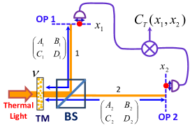
Figure 1: (color online). The traditional HBT scheme. The TM is in front of the beam splitter (BS), and the intensities on the output planes (OPs) 1 and 2 are correlated by a correlator. Optical paths 1 (2) from the TM to the OPs 1 (2) are characterized by the $2\times 2$ ray transfer matrices.

We first briefly discuss the traditional HBT scheme HanburyBrown1956 ; AlQasimi2010 , see Fig. 1. The light passes through the TM, and then it is divided into two paths by the beam splitter (BS). It is known that, for thermal or incoherent sources obeying Gaussian statistics, the intensity-intensity correlation $C_{T}(x_{1},x_{2})$ is expressed by Siegert relation Saleh1978

$$C_{T}(x_{1},x_{2})=\left\langle I_{T}(x_{1})\right\rangle\left\langle I_{T}(x_{2})\right\rangle+\left|W_{T}(x_{1},x_{2})\right|^{2},$$ (1)

where $\left\langle I_{T}(x_{j})\right\rangle$ ($j=1,2$) are the average intensities on the output planes, $W_{T}(x_{1},x_{2})$ is the cross-spectral density between the two output planes, and they are respectively given by Saleh2000

$$\left\langle I_{T}(x_{j})\right\rangle\!=\!\!\!\iint\!\!\!W_{i}(\nu_{1},\nu_{2})h_{j}^{\ast}(\nu_{1},x_{j})h_{j}(\nu_{2},x_{j})d\nu_{1}d\nu_{2},$$ (2)

$$\!W_{T}(x\!_{1}\!,x_{2})\!=\!\!\!\iint\!\!\!W_{i}(\nu_{1}\!,\!\nu_{2})h_{1}^{\ast}(\nu_{1}\!,\!x_{1})h_{2}(\nu_{2}\!,\!x_{2})d\nu_{1}d\nu_{2}.$$ (3)

Here $W_{i}(\nu_{1},\nu_{2})\equiv\left\langle E_{i}^{\ast}(\nu_{1})E_{i}(\nu_{2})\right\rangle$ is the initial cross-spectral density of the input random light fields $E_{i}(\nu)$ at the TM. The impulse response functions $h_{j}(\nu,x_{j})$, from the Collins’ formula, can be expressed as Collins1970 ; WangSMZhaoDM

$$h_{j}(\nu,x_{j})=t(\nu)(\frac{-i}{\lambda B_{j}})^{\frac{1}{2}}e^{\frac{i\pi}{\lambda B_{j}}(A_{j}\nu^{2}-2\nu x_{j}+D_{j}x_{j}^{2})}$$ (4)

under the paraxial approximation, where $\lambda$ is the wavelength, $A_{j}$, $B_{j}$, and $D_{j}$ are the elements of the $2\times 2$ ray transfer matrices $\left(\begin{array}[]{cc}A_{j}&B_{j}\\ C_{j}&D_{j}\end{array}\right)$ describing the linear optical systems Milonni2010 from the TM to the output planes, and $t(\nu)$ is the complex transmission coefficient of the TM.

For simplicity, both optical paths 1 and 2 are assumed to be within the range of Fraunhofer diffraction WangSMZhaoDM , i. e., $A_{j}=0$. Meanwhile, the input light is a thermal or incoherent source, i. e., $W_{i}(u_{1},u_{2})=I_{0}\delta(u_{1}-u_{2})$ with $I_{0}$ a constant. Therefore, $C_{T}(x_{1},x_{2})$ can be written as

$$C_{T}(x_{1},x_{2})=\left\langle I_{T}(x_{1})\right\rangle\left\langle I_{T}(x_{2})\right\rangle\left[1+\mu_{T}(x_{1},x_{2})\right],$$ (5)

where

$$\mu_{T}(x_{1},x_{2})=\frac{1}{N_{0}^{2}}\left|\tciFourier_{1}\left[\left|t(u)\right|^{2}\right](\frac{x_{2}}{\lambda B_{2}}-\frac{x_{1}}{\lambda B_{1}})\right|^{2}$$ (6)

is the normalized phase-insensitive shape function. This shape function is only related to $\left|t(\nu)\right|^{2}$, $\left\langle I_{T}(x_{j})\right\rangle=I_{0}N_{0}(\lambda\left|B_{j}\right|)^{-1}$ with $N_{0}=\int\left|t(\nu)\right|^{2}d\nu$, and $\tciFourier_{1}$ denotes the one-dimensional Fourier transform of $\left|t(\nu)\right|^{2}$ with the argument of $\frac{x_{2}}{\lambda B_{2}}-\frac{x_{1}}{\lambda B_{1}}$. It is clear that $\mu_{T}(x_{1},x_{2})$ contains only the partial information of $t(\nu)$ [i. e., the amplitude of $t(\nu)$], and it does not have any phase information of $t(\nu)$. Therefore, the thermal intensity-intensity correlations based on the traditional HBT scheme are essentially phase insensitive Peeters2010 ; Erkmen2008 . It should be emphasized that both $\left\langle I_{T}(x_{1})\right\rangle$ and $\left\langle I_{T}(x_{2})\right\rangle$ are uniform and have no any information of $t(\nu)$ for completely incoherent fields.

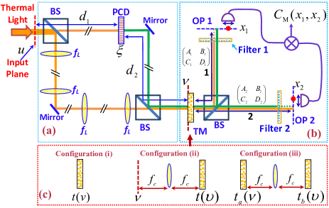
Figure 2: (Color) The modified HBT scheme for demonstrating the intensity-correlation speckle with the phase-sensitive effects by using thermal light fields. Part (a) provides the modified thermal source at the incident plane ($\nu$) of the TM. In the upper path of (a), the random light fields pass through a forward non-degenerated PC device (PCD), and the optical distances $d_{1}$($d_{2}$) between the input plane (the PCD) and the PCD (the TM) are adjustable in order for generating the conjugated fields at the incident plane ($\nu$) of the TM. In the lower path of (a), the random light fields pass through two pairs of 4-$f$ optical systems, which directly image the thermal light fields onto the incident plane of the TM. Part (b) provides the intensity-correlation measurements similar to the case of Fig. 1, except for the filters added in each arm. Part (c) shows three configurations (i)-(iii) for displaying three different intensity-correlation speckles.

In order to overcome the limit of the traditional HBT-based scheme, we design a new optical system to fulfill the phase-sensitive intensity-intensity correlation scheme for thermal light, as shown in Fig. 2. The thermal fields first pass through the optical systems in Fig. 2(a), for generating the modified thermal source at the incident plane ($\nu$) of the TM [in Fig. 2(b)]. A forward non-degenerated phase conjugation (PC) device HeGS2002 is inserted into the upper path in Fig. 2(a), and it generates the PC waves with wavelength $\lambda_{p}$ (here $\lambda_{p}\neq\lambda$). When $\lambda d_{1}=\lambda_{p}d_{2}$, where $d_{1}$ ($d_{2}$) are the distances from the input plane $u$ (the PC device) to the PC device (the TM), then the random light at the TM via the upper path forms a conjugated image of the input light, i. e., $E_{\nu,\text{up}}(\nu)=\alpha E_{i}^{\ast}(\nu)$ Note02 , where $\nu$ is the coordinate on the incident plane of the TM, and $\alpha$ is the rate of generating the PC light. In the lower path of Fig. 2(a), it consists of two pairs of $4-f$ optical systems Goodman1996 ; Pedrotti2007 with the same focus length $f_{L}$. Thus, the light at the TM via the lower optical path is the same as the input field, i. e., $E_{\nu,\text{low}}(\nu)=E_{i}(\nu)$ Note02 . In Fig. 2(b), it displays the measurement diagram of the intensity-intensity correlation, and the total light fields from both two paths of Fig. 2(a) pass through the common TM. The subsystems from the TM to two output planes 1 and 2 also lie in Fraunhofer region (i. e., $A_{j}=0$) WangSMZhaoDM , and they are the same as those in Fig.1 except for the additional optical filters. The filters 1 and 2 transmit the light fields of wavelength $\lambda_{p}$ and $\lambda$, respectively, while blocking the remainder in each arm. Therefore, the intensity-intensity correlation in the modified system can also be derived from its definition: $C_{M}(x_{1},x_{2})\equiv\left\langle I_{M}(x_{1})I_{M}(x_{2})\right\rangle$ MandelWolf , where $I_{M}(x_{1,2})$ are the instantaneous intensities on each output plane. It is the correlation between the original random light fields and their PC fields that leads to the phase-sensitive term. Thus, $C_{M}(x_{1},x_{2})$ now can be written as Note03

$$C_{M}(x_{1},x_{2})=\left\langle I_{M}(x_{1})\right\rangle\left\langle I_{M}(x_{2})\right\rangle[1+\mu_{M}^{(p)}(x_{1},x_{2})],$$ (7)

where $\mu_{M}^{(p)}(x_{1},x_{2})=|W_{M}^{(p)}(x_{1},x_{2})|^{2}/[\left\langle I_{M}(x_{1})\right\rangle\left\langle I_{M}(x_{2})\right\rangle]$ is the normalized phase-sensitive shape function and it is dependent on the detailed configuration of the optical system containing the TM [see Fig. 2(c)], and $W_{M}^{(p)}\!(x_{1},x_{2}\!)\!\!=\!\!\alpha\iint\!\!W_{i}\!(\nu_{1},\nu_{2}\!)h_{1}\!(\nu_{1},x_{1}\!)h_{2}\!(\nu_{2},x_{2}\!)d\nu_{1}\!d\nu_{2}$ is the phase-sensitive cross-spectral density between the two output planes in Fig. 2(b). Actually, $\mu_{M}^{(p)}(x_{1},x_{2})$ determines the main behavior of $C_{M}(x_{1},x_{2})$ since the common factor $\left\langle I_{M}(x_{1})\right\rangle\left\langle I_{M}(x_{2})\right\rangle$ is separable.

Next we present the results for three configurations with thermal light, as shown in Fig. 2(c), demonstrating the similar features as two-photon speckle patterns Peeters2010 , although the calculation is tedious but straightforward.

In the configuration (i), the TM is located at the common imaging position of both paths of Fig. 2(a). In this case, $\mu_{M}^{(p)}(x_{1},x_{2})$ in Eq. (7) is given by Note04

$$\mu_{M}^{(p)}(x_{1},x_{2})=\frac{1}{N_{0}^{2}}\left|\tciFourier_{1}\left[t^{2}(\nu)\right](\frac{x_{1}}{\lambda_{p}B_{1}}+\frac{x_{2}}{\lambda B_{2}})\right|^{2}.$$ (8)

It is clear that $\mu_{M}^{(p)}(x_{1},x_{2})$ has a different form compared to Eq. (6) as $|t(\nu)|^{2}$ is replaced by $t^{2}(\nu)$. The modified intensity-intensity correlation in this case naturally contains all phase-sensitive information of $t(\nu)$. Here the average output intensities are $\left\langle I_{M}(x_{1})\right\rangle=I_{0}N_{0}\alpha^{2}(\lambda_{p}\left|B_{1}\right|)^{-1}$ and $\left\langle I_{M}(x_{2})\right\rangle=I_{0}N_{0}(\lambda\left|B_{2}\right|)^{-1}$, which are constants and can also be subtracted from the measurement of $C_{M}(x_{1},x_{2})$. When $\lambda_{p}B_{1}=\lambda B_{2}$, Eq. (8) becomes $\mu_{M}^{(p)}(x_{1},x_{2})=N_{0}^{-2}\left|\tciFourier_{1}\left[t^{2}(\nu)\right](\frac{x_{1}+x_{2}}{\lambda_{p}B_{1}})\right|^{2}$, i. e., a function of the sum coordinate $x_{1}+x_{2}$. This property is the same as that of the two-photon speckle for the configuration (a) in Ref. Peeters2010 .

In the configuration (ii), the TM is placed at the exit plane of a 2-$f$ Fourier optical system with the focus length $f_{c}$ Goodman1996 ; Pedrotti2007 , so that $\mu_{M}^{(p)}(x_{1},x_{2})$ is given by Note04

$$\mu_{M}^{(p)}(x_{1},x_{2})=\frac{\lambda_{p}}{\lambda N_{0}^{2}}\left|\tciFourier_{1}\left[\Omega(\upsilon)\right](\frac{x_{2}}{\lambda B_{2}}-\frac{x_{1}}{\lambda B_{1}})\right|^{2},$$ (9)

where $\Omega(\upsilon)=t(\upsilon)t(-\frac{\lambda_{p}}{\lambda}\upsilon)$ is a phase-sensitive function. From Eq. (9), the phase sensitive effect comes from the Fourier transformation of $\Omega(\upsilon)$. The average intensities here are the same as that of the configuration (i). Different from the previous case, when $B_{1}=B_{2}$, Eq. (9) can be rewritten as $\mu_{M}^{(p)}(x_{1},x_{2})=\frac{\lambda_{p}}{\lambda N_{0}^{2}}\left|\tciFourier_{1}\left[\Omega(\upsilon)\right](\frac{x_{2}-x_{1}}{\lambda B_{1}})\right|^{2}$, which is a function of the difference coordinate $x_{2}-x_{1}$. This property is also similar to that of the two-photon speckle for the configuration (b) in Ref. Peeters2010 .

For the configuration (iii), two TMs are located at the incident and exit planes of the 2-$f$ Fourier optical system with the same $f_{c}$. As pointed out in Ref. Peeters2010 , this configuration mimics a volume scatterer. By a tedious but straightforward calculation, $\mu_{M}^{(p)}(x_{1},x_{2})$ is given by Note04

$$\mu_{M}^{(p)}(x_{1},x_{2})=\frac{\left|\tciFourier_{2}\left[\Theta_{p}(\upsilon_{1},\upsilon_{2})\right](\frac{x_{1}}{\lambda_{p}B_{1}},\frac{x_{2}}{\lambda B_{2}})\right|^{2}}{S(x_{1})S(x_{2})},$$ (10)

where $\tciFourier_{2}$ denotes the two-dimensional Fourier transform, $\Theta_{p}(\upsilon_{1},\upsilon_{2})=\eta t_{b}(\upsilon_{1})t_{b}(\upsilon_{2})\tciFourier_{1}[t_{a}^{2}(\nu)](\frac{\upsilon_{1}}{\lambda_{p}f_{c}}+\frac{\upsilon_{2}}{\lambda f_{c}})$ with $\eta=f_{c}^{-1}(\lambda_{p}\lambda)^{-1/2}$, and $S(x_{j})=\tciFourier_{2}[\Theta_{n,j}(\upsilon_{1},\upsilon_{2})](-\frac{x_{j}}{\lambda_{j}B_{j}},\frac{x_{j}}{\lambda_{j}B_{j}})$ with $\Theta_{n,j}(\upsilon_{1},\upsilon_{2})=(\lambda_{j}f_{c})^{-1}t_{b}^{\ast}(\upsilon_{1})t_{b}(\upsilon_{2})\tciFourier_{1}[\left|t_{a}(\nu)\right|^{2}](\frac{\upsilon_{2}-\upsilon_{1}}{\lambda_{j}f_{c}})$. Here $t_{a}(\nu)$ and $t_{b}(\upsilon)$ are the complex transmission coefficients for the two TMs, respectively; and the output average intensities are $\left\langle I_{M}(x_{1})\right\rangle=\alpha^{2}I_{0}(\lambda_{p}\left|B_{1}\right|)^{-1}S(x_{1})$ and $\left\langle I_{M}(x_{2})\right\rangle=I_{0}(\lambda\left|B_{2}\right|)^{-1}S(x_{2})$, which are not constant any more. It is clear that $\Theta_{p}(\nu_{1},\nu_{2})$ includes all phase information of both $t_{a}(\nu)$ and $t_{b}(\upsilon)$, while $\Theta_{n,j}(\upsilon_{1},\upsilon_{2})$ are phase insensitive and they are only related to the average intensities. The difference between $\Theta_{p}(\upsilon_{1},\upsilon_{2})$ and $\Theta_{n,j}(\upsilon_{1},\upsilon_{2})$ is the key point for generating the phase-sensitive effect of the intensity-intensity correlation patterns for the volume scattering phenomena in this modified HBT scheme.

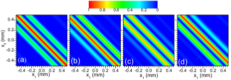
Figure 3: (Color) Dependence of $\mu_{M}^{(p)}(x_{1},x_{2})$ on the phase of one of double slits. (a) $\phi=0$ or $\pi$, (b) $\phi=\pi/4$, (c) $\phi=\pi/2$, and (d) $\phi=3\pi/4$. Other parameters are $\lambda_{p}B_{1}=\lambda B_{2}=0.25$ mm², $a=0.5$ mm, and $b=1.0$ mm.

From the above cases, all phase information of the TMs is included in the function $\mu_{M}^{(p)}(x_{1},x_{2})$ although different configurations may have different specific forms. In order to understand the phase sensitive effect in our modified scheme, we first consider a simple example–the double slits in the configuration (i) of Fig. 2(c). The complex value of $t(\nu)$ for the double slits is given in Ref. Note05 . After substituting $t(\nu)$ into Eq. (8), we obtain $\mu_{M}^{(p)}(x_{1},x_{2})=\sin^{2}\left[\phi+\pi d(\frac{x_{1}}{\lambda_{p}B_{1}}+\frac{x_{2}}{\lambda B_{2}})\right]\operatorname{sinc}^{2}\left[\pi a(\frac{x_{1}}{\lambda_{p}B_{1}}+\frac{x_{2}}{\lambda B_{2}})\right]$, where $a$ is the slit width, $d$ the slit separation, and $\phi$ the phase of one slit. It is clear that the phase $\phi$ has the influence on the distribution $\mu_{M}^{(p)}(x_{1},x_{2})$ [see Fig. 3], and different values of $\phi$ correspond to different intensity-intensity correlation interference patterns. From Eq. (7), due to the background term, the maximal visibility of the intensity-intensity correlation interference pattern is equal to 1/3 for the cases $\phi=m\pi$ with $m$ being an integer. Thus, we obtain different visibility for different $\phi$. Here only the distributions of $\mu_{M}^{(p)}(x_{1},x_{2})$ are demonstrated since the background term $\left\langle I_{M}(x_{1})\right\rangle\left\langle I_{M}(x_{2})\right\rangle$ can be subtracted from the intensity correlation, like the situations in thermal ghost imaging and interference Bennink2002 ; Bennink2004 ; Gatti2004 ; YanhuaShih2007 .

We now discuss the intensity-intensity correlation speckle patterns of the thermal light passing through the different configurations in Fig. 2. Figure 4 shows the effect of the phase distribution of $t(\nu)$ on the distribution of $\mu_{M}^{(p)}(x_{1},x_{2})$ for three different diffusers in the configuration (i). The random amplitude and phase distributions of three diffusers are correspondingly shown at the upper parts in Figs. 4(a)-4(c). Note that the values of $\left|t(\nu)\right|$ in Figs. 4(a)-4(c) are the same, while their phase magnitudes are totally different. It is seen that the patterns of $\mu_{M}^{(p)}(x_{1},x_{2})$ vary with changing the phase distributions of $t(\nu)$, and the more randomness of the phase distributions may lead to the more homogeneous interference speckle patterns with the smaller average speckle size.

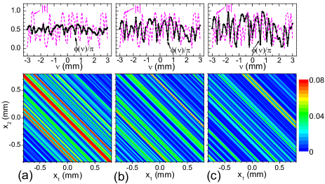
Figure 4: (Color) Different distributions of $\mu_{M}^{(p)}(x_{1},x_{2})$ for three different random diffusers in the configuration (i) of Fig. 2(c). The corresponding upper parts show the amplitude and phase distributions of three different TMs. Other parameters are $\lambda_{p}B_{1}=\lambda B_{2}=0.25$ mm².

In Fig. 5, we demonstrate the patterns of $\mu_{M}^{(p)}(x_{1},x_{2})$ for the diffusers in (a) the configuration (ii), and (b-c) the configuration (iii). The functions of the TMs in these simulations are the same as that in Fig. 4(c). Comparing with Fig. 4(c), the pattern in Fig. 5(a) is along with the difference coordinate $x_{1}-x_{2}$ not along with the sum coordinate $x_{1}+x_{2}$. Such changes are similar to the cases in two-photon speckle Peeters2010 , and they cannot happen in the traditional HBT scheme with thermal light. From Figs. 5(b-c), for the configuration (iii), the patterns of $\mu_{M}^{(p)}(x_{1},x_{2})$ mimic the volume scatterer, and the nonfactorizable features in the correlation patterns are clearly seen. For a small value of $f_{c}$ in Fig. 5(c), the correlation speckle spots in the pattern of $\mu_{M}^{(p)}(x_{1},x_{2})$ are elongated along the difference coordinate of $x_{1}-x_{2}$. This can be understood from the fact that the second diffuser is illuminated with the far-field patterns of the first diffuser. Within the same area of the second diffuser, the smaller of $f_{c}$, the less information from the first diffuser can be projected. This can be seen from the form of the function $\Theta_{p}(\nu_{1},\nu_{2})$. Therefore, we can conclude that the modified HBT scheme with thermal light can provide the phase-sensitive intensity-intensity correlation speckle.

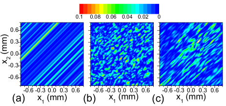
Figure 5: (Color) Distributions of $\mu_{M}^{(p)}(x_{1},x_{2})$ for the random diffusers in the cases of (a) the configuration (ii), and (b-c) the configuration (iii). Other parameters are $\lambda_{p}=550$nm, $\lambda=500$nm, $B_{1}=B_{2}=500$ mm, $f_{c}=500$mm for (b) and $150$mm for (c).

Lastly, we discuss the possibility of experimentally realizing our scheme. The key challenge of our scheme in Fig. 2 is to generate the non-degenerate PC fields of thermal light. For demonstrating our predicted result, one can employ the psudothermal light source (produced via the random scattering when a laser field passes through a ground glass) as the input light. The PC light of the psudothermal light can be generated via the conventional PC technologies, such as the four-wave mixing processes (e. g., Refs. Hellwarth1977 ; Bloom1977 ; Heer1979 ; Khyzniak1984 ) and the stimulated scattering processes (e. g., Refs. Yu1972 ; Wang1978 ; Mullen1992 ; Bowers1998 ). For example, the nondegenerate PC light is generated by using a Pr³⁺:Y₂SiO₅ crystal based on the electromagnetically induced transparency effect ZhaiZH2011 . Meanwhile, the fidelity of the PC fields may have an influence on the correlations between the input and PC fields, and this will in turn affect the intensity-intensity correlations. In another scheme, we can use the novel digital PC technology Cui2010 ; Hsieh2010 ; Wang2012 ; Hillman2013 , which does not involve the nonlinear processes and can even generate the high-quality PC waves for the weak, incoherent fluorescence signal Vellekoop2013 , to verify this effect. In fact, if the filters in Fig. 2(b) are removed or disabled (when $\lambda_{p}=\lambda$), both the phase-sensitive and phase-insensitive terms will occur in Eq. (7), which only increases the complexity to determine the phase-sensitive patterns.

In summary, we have presented the phase-sensitive intensity-intensity correlation speckle effect of thermal light in the modified HBT scheme. This scheme is based on introducing the PC light to change the correlations between the two optical paths. It is revealed that the phase-sensitive and nonfactorizable features can be seen in thermal intensity-intensity correlation speckle. Finally, the discussion on the experimental realization is presented. This scheme is different from those thermal ghost imaging and diffraction Bennink2002 ; Bennink2004 ; Gatti2004 ; YanhuaShih2007 ; Borghi2006 and the unbalanced interferometer-based scheme via the direct intensity measurements Zhang2009 , since all thermal photons in our case pass through the common sample. Our scheme can also be used to recover the phase information in the thermal-like temporal intensity-intensity correlation cases Torres-Company2012 . This modified HBT scheme may have important applications for developing the intensity-intensity correlation speckle and imaging technologies of thermal or incoherent light sources.

- (1) J. W. Goodman, Speckle Phenomena in Optics (Roberts and Company, Englewood, CO, 2007).
- (2) U. Bortolozzo, S. Residori, and P. Sebbah, Phys. Rev. Lett. 106, 103903 (2011).
- (3) C. W. J. Beenakker, J. W. F. Venderbos, and M. P. van Exter, Phys. Rev. Lett. 102, 193601 (2009).
- (4) M. Candé and S. E. Skipetrov, Phys. Rev. A 87, 013846 (2013).
- (5) W. H. Peeters, J. J. D. Moerman, and M. P. van Exter, Phys. Rev. Lett. 104, 173601 (2010).
- (6) M. P. van Exter, J. Woudenberg, H. Di Lorenzo Pires, and W. H. Peeters, Phys. Rev. A 85, 033823 (2012).
- (7) H. Di Lorenzo Pires, J. Woudenberg, and M. P. van Exter, Phys. Rev. A 85, 033807 (2012).
- (8) R. S. Bennink, S. J. Bentley, and R. W. Boyd, Phys. Rev. Lett. 89, 113601 (2002).
- (9) R. S. Bennink, S. J. Bentley, R. W. Boyd, and J. C. Howell, Phys. Rev. Lett. 92, 033601 (2004).
- (10) A. Gatti, E. Brambilla, M. Bache, and L. A. Lugiato, Phys. Rev. Lett. 93, 093602 (2004).
- (11) Y. Cai and S. Y. Zhu, Opt. Lett. 29, 2716 (2004).
- (12) K. Wang and D. Z. Cao, Phys. Rev. A 70, 041801(R) (2004).
- (13) F. Ferri, D. Magatti, A. Gatti, M. Bache, E. Brambilla, and L. A. Lugiato, Phys. Rev. Lett. 94, 183602 (2005).
- (14) Y. H. Zhai, X. H. Chen, D. Zhang, and L. A. Wu, Phys. Rev. A 72, 043805 (2005).
- (15) B. E. A. Saleh, A. F. Abouraddy, A. V. Sergienko, and M. C. Teich, Phys. Rev. A 62, 043816 (2000).
- (16) B. I. Erkmen and J. H. Shapiro, Phys. Rev. A 78, 023835 (2008).
- (17) R. Hanbury Brown and R. Q. Twiss, Nature 178, 1046 (1956).
- (18) A. Al-Qasimi, M. Lahiri, D. Kuebel, D. F. V. James, and E. Wolf, Opt. Exp. 18, 17124 (2010).
- (19) B. E. A. Saleh, Photoelectron Statistics (Springer, New York, 1978).
- (20) S. A. Collins, J. Opt. Soc. Am. 60, 1168 (1970).
- (21) S. Wang and D. Zhao, Matrix Optics (Springer-Verlag, Berlin, 2000)
- (22) P. W. Milonni and J. H. Eberly, Laser Physics (John Wiley & Sons, Hoboken, NJ, 2010).
- (23) G. S. He, Progress in Quantum Electronics 26, 131-191 (2002).
- (24) See Supplemental Material at [URL will be inserted by publisher] for the derivation of the light fields at the incident plane of the transmission mask. Here is the function of the input field at the input plane , see Fig. 2.
- (25) J. W. Goodman, Introduction to Fourier Optics (2nd Edition) (McGraw-Hill, New York, 1996).
- (26) F. L. Pedrotti, L. M. Pedrotti, and L. S. Pedrotti, Introduction to Optics (San Francisco: Pearson Prentice-Hall, 2007).
- (27) L. Mandel and E. Wolf, Optical Coherence and Quantum Optics (Cambridge University Press, Cambridge, England, 1995).
- (28) See Supplemental Material at [URL will be inserted by publisher] for the derivation of Eq. (7).
- (29) See Supplemental Material at [URL will be inserted by publisher] for the derivation of Eqs. (8)-(10).
- (30) For the phase-dependent double slits, the transmission coefficient here is defined by for , and for , otherwise , where is the slit width, () is the separation of two slits, and is the phase of one slit.
- (31) Y. Shih, “Quantum imaging”, IEEE Journal of Selected Topics in Quant. Electronics 13, 1016 (2007).
- (32) R. W. Hellwarth, J. Opt. Soc. Am. 67, 1 (1977).
- (33) D. M. Bloom and G. C. Bjorkund, Appl. Phys. Lett. 31, 592 (1977).
- (34) C. V. Heer and N. C. Griffen, Opt. Lett. 4, 239 (1979).
- (35) A. Khyzniak, V. Kondilenko, Y. Kucherov, S. Lesnik, S. Odoulov, and M. Soskin, J. Opt. Soc. Am. A 1, 169 (1984).
- (36) O. Y. Nosach, V. I. Popovichev, V. V. Ragul’skii, and F. S. Faizullov, JETP Lett. 16, 435 (1972).
- (37) V. Wang and C. R. Giuliano, Opt. Lett. 2, 4 (1978).
- (38) R. A. Mullen, D. J. Vickers, L. West, and D. M. Pepper, J. Opt. Soc. Am. B 9, 1726 (1992).
- (39) M. W. Bowers and R. W. Boyd, IEEE J. of Quant. Electronics 34, 634 (1998).
- (40) Z. Zhai, Y. Dou, J. Xu, and G. Zhang, Phys. Rev. A 83, 043825 (2011).
- (41) M. Cui and C. Yang, Opt. Express 18, 3444 (2010).
- (42) C. L. Hsieh, Y. Pu, R. Grange, G. Laporte, and D. Psaltis, Opt. Express 18, 20723 (2010).
- (43) Y. M. Wang, B. Judkewitz, C. A. DiMarzio, and C. Yang, Nature Communications 3, 928 (2012).
- (44) T. R. Hillman, T. Yamauchi, W. Choi, R. R. Dasari, M. S. Feld, Y. Park, and Z. Yaqoob, Scientific Reports 3, 1909 (2013).
- (45) I. M. Vellekoop, M. Cui, and C. Yang, Appl. Phys. Lett. 101, 081108 (2012).
- (46) R. Borghi, F. Gori, and M. Santarsiero, Phys. Rev. Lett. 96, 183901 (2006).
- (47) S. -H. Zhang, L. Gao, J. Xiong, L. -J. Feng, D. -Z. Cao, and K. Wang, Phys. Rev. 102, 073904 (2009).
- (48) V. Torres-Company, J. P. Torres, and A. T. Friberg, Phys. Rev. Lett. 109, 243905 (2012).