Dynamical diffusion and renormalization group equation for the Fermi velocity in doped graphene

Abstract

The aim of this work is to study the electron transport in graphene with impurities by introducing a generalization of linear response theory for linear dispersion relations and spinor wave functions. Current response and density response functions are derived and computed in the Boltzmann limit showing that in the former case a minimum conductivity appears in the no-disorder limit. In turn, from the generalization of both functions, an exact relation can be obtained that relates both. Combining this result with the relation given by the continuity equation, is possible to obtain general functional behavior of the the diffusion pole. Finally, a dynamical diffusion is computed in the quasistatic limit using the definition of relaxation function. A lower cutoff must be introduce to regularize infrared divergences which allows to obtain a full renormalization group equation for the Fermi velocity, which is solved up to order $O(\hbar^{2})$.

1 Introduction

Graphene is a two dimensional hexagonal lattice of carbon atoms and is one of the most important topics in solid state physics due to the vast application in nano-electronics, opto-electronics, superconductivity and Josephson junctions ([1],[2],[3],[4] and [5]). The band structure shows that the conduction and valence band touch at the Dirac point and the dispersion relation is approximately linear and isotropic [6]. This linear dispersion near the symmetry points have striking similarities with those of massless relativistic Dirac fermions [4]. This leads to a number of fascinating phenomena such as the half-quantized Hall effect ([7],[8]) and minimum quantum conductivity in the limit of vanishing concentration of charge carriers [1]. Although this is an outstanding experimental result, there is no consensus about the theoretical value computed through different theoretical methods (see [9]), neither the physical reason for such minimum value (see [10]), where the minimum is due to the impurity resonance and is not related to the Dirac point.

In particular, one of the theoretical methods used to compute response functions within the linear response theory is the Kubo formalism [11]. Deviations of charge and current densities from their equilibrium values are described by density and current response functions through Kubo formulas using the same two-particle Green function. Although, generally is unable to obtain exact relations between these response functions, several approximations can be obtained taking into account the dimensionality and dispersion relation of the system (see [12]). But these approximate relations are based on the continuity equation and Ward identities and is not clear if these assumptions are valid for linear dispersion relations and spinor wave functions.

In turn, impurities in graphene can be considered in various type of forms: substitutional, where the site energy is different from those of carbon atoms, which originates resonances [13] and as adsorbates, that can be placed on various points in graphene; sixfold hollow site of a honeycomb lattice, twofold bridge site of two neighboring carbons or top site of a carbon atom [14]. Theoretical as well as experimental studies have indicated that substitutional doping of carbon materials can be used to tailor their physical and/or chemical properties ([15], [16], [17]). In particular, nitrogen or boron dopants can be added to pristine graphene ([18],[19],[20],[21]).

The detection and absorption of low levels of hydrogen becomes very important for sensor gas and hydrogen energy. Different methods of hydrogen detection are not entirely selective or it have a high cost of manufacture due to their complexity. Pd-doped reduced graphene have a clear response to hydrogen and are very selective ([22], [23]). In the other side, the decoration of carbon support by transition metals can also be independently used to enhance the hydrogen storage of the specimens. Transition metals eliminate the hydrogen dissociation barrier altogether [24].

In this sense, the density and current response function of doped-graphene with low concentration of subtitutional impurities is of major importance for the consequences in the sensor effect ([25], [26]). In particular, the simplest graphene-based sensor detects the conductivity change upon adsorption of analyte molecules. The change of conductivity could be attributed to the changes of charge carrier concentration in the graphene induced by adsorbed gas molecules. It has been proposed that such device may be capable of detecting individual molecule [27]. These reactions release captured electrons in the interaction zone between the gas and the sensor, and increase their concentration in the conductivity zone. But the conductivity of electrons are based on the diffusion phenomena of charge carriers through the sample. Electrons moving in randomly distributed scatterers has a diffusive character, which is described at long distances by a diffusion equation. It has been shown that it is possible to supress diffusion (see [28]), giving rise to a localization phenomena, which will affect the sensor characteristics of the material. In turn, a dynamical generalization of the diffusion constant from the electron-hole correlation function cannot be linked to the frequency dependent conductivity (see eq.(3.18) and eq.(3.19) of [12]). In this sense, the aim of this work is two-fold: to introduce a generalization of the linear response theory for linear dispersion relation and spinor wave functions, to apply it to graphene, and the subsequent computation of minimal conductivity and dynamical diffusion, to analize the general behavior of the system under local perturbations and the implications for sensor gas.

This work will be organized as follow: In section II, the impurity averaged Green function will be computed. In section III and IV, a generalization of the conductivity tensor and response function will be computed using the current definition for relativistic Dirac fermions. In section V, different limit behavior of the current and density response functions are computed. The Boltzmann limit is introducedshowing the minimal conductivity value. In section VI, the dynamical diffusion will be computed through the relaxation function, showing how the obtain the full renormalization group equation for the Fermi velocity. Finally, the conclusion are presented. Appendix A and B are introduced for self-contained lecture.

2 Impurity averaged Green function

The Hamiltonian of clean graphene in the $K$ point in the Brillouin zone and in the long wavelength approximation reads (see [4])

$$H=v_{F}\left(\begin{array}[]{cc}0&p_{x}+ip_{y}\\ p_{x}-ip_{y}&0\end{array}\right)$$ (1)

where $v_{F}\sim 10^{6}m/s$ is the Fermi velocity. The eigenfunctions of this Hamiltonian reads

$$\psi_{\mathbf{k}}(\mathbf{r})=\frac{1}{\sqrt{2}}\left(\begin{array}[]{c}1\\ \lambda e^{i\varphi_{\mathbf{k}}}\end{array}\right)e^{i\mathbf{k}\cdot\mathbf{r}}$$ (2)

where

$$\varphi_{\mathbf{k}}=\arctan(\frac{k_{y}}{k_{x}})$$ (3)

In turn, the eigenvalues reads

$$E_{\lambda}(\mathbf{k})=\lambda v_{f}\hbar k$$ (4)

where $k=\left|\mathbf{k}\right|$ and where $\lambda=1$ are positive energy states (conduction band) and $\lambda=-1$ are negative energy states (valence band).With the eigenfunctions of eq.(2) we can compute the retarded and advanced Green function for conduction electrons $(\lambda=1)$ in momentum space

$$G_{0}^{R(A)}(\mathbf{q},E)=\frac{1}{E-v_{f}\hbar q\mp is}\left(\begin{array}[]{cc}1&e^{i\varphi_{\mathbf{q}}}\\ e^{-i\varphi_{\mathbf{q}}}&1\end{array}\right)$$ (5)

where the minus sign correspond to the retarded Green function and the plus sign to the advanced Green function. The contribution to second order in the perturbation expansion in the impurity potential reads (see [29], eq.(3.31), page 136)

$$\left\langle G_{2}^{R}(\mathbf{k},\mathbf{k}^{\prime},E)\right\rangle^{i=j}=\delta_{\mathbf{k,k}^{\prime}}n_{i}[G_{0}^{R}(\mathbf{k},E)]^{2}\int\frac{d^{2}\mathbf{k}^{\prime}}{(2\pi)^{2}}\left|V_{imp}(\mathbf{k}-\mathbf{k}^{\prime})\right|^{2}IG_{0}^{R}(\mathbf{k}^{\prime},E)$$ (6)

where $n_{i}$ is the impurity concentration, $\left|V_{imp}(\mathbf{k}-\mathbf{k}^{\prime})\right|^{2}I$ is a diagonal matrix

$$\left|V_{imp}(\mathbf{k}-\mathbf{k}^{\prime})\right|^{2}I=\left(\begin{array}[]{cc}\left|V_{imp}(\mathbf{k}-\mathbf{k}^{\prime})\right|^{2}&0\\ 0&\left|V_{imp}(\mathbf{k}-\mathbf{k}^{\prime})\right|^{2}\end{array}\right)$$ (7)

and the angle brackets represent the configurational averaging that can be computed as

$$\left\langle A\right\rangle=\int\overset{N}{\underset{i=1}{\prod}}d\mathbf{r_{i}}A(\mathbf{r_{1},r_{2},...,r_{N}})P(\mathbf{r_{1},r_{2},...,r_{N}})$$ (8)

where $P(\mathbf{r_{1},r_{2},...,r_{N}})=P(\mathbf{r_{1}})P(\mathbf{r_{2}})...P(\mathbf{r_{N}})$ and $P(\mathbf{r_{i}})$ is the probability density for having the impurity located around point $\mathbf{r_{i}}$. In eq.(6), the Fourier transform of $G_{2}^{R}(\mathbf{r},\mathbf{r}^{\prime},E)~{}$has been taken first. Replacing last equation and eq.(5) in eq.(6) the diagonal part of the averaged Green function reads

$$\int\frac{d^{2}\mathbf{k}^{\prime}}{(2\pi)^{2}}\frac{\left|V_{imp}(\mathbf{k}-\mathbf{k}^{\prime})\right|^{2}}{E-v_{f}\hbar k^{\prime}-is}=$$ (9)

$$\int\frac{d^{2}\mathbf{k}^{\prime}}{(2\pi)^{2}}\left|V_{imp}(\mathbf{k}-\mathbf{k}^{\prime})\right|^{2}\left(\frac{E-v_{f}\hbar k^{\prime}}{(E-v_{f}\hbar k^{\prime})^{2}+s^{2}}+i\frac{s}{(E-v_{f}\hbar k^{\prime})^{2}+s^{2}}\right)$$

If we consider for simplicity that the impurity potential is a Dirac delta potential, then

$$V_{imp}(\mathbf{k})=\int d^{2}\mathbf{r}e^{-i\mathbf{r}\cdot\mathbf{q}}V_{imp}(\mathbf{r})=\int d^{2}\mathbf{r}e^{-i\mathbf{r}\cdot\mathbf{q}}V_{0}\delta(\mathbf{r})=V_{0}$$ (10)

Using the last result, the integral of eq.(9) reads

$$V_{0}^{2}\underset{s\rightarrow 0}{\lim}\int\frac{d^{2}\mathbf{k}^{\prime}}{(2\pi)^{2}}\left(\frac{E-v_{f}\hbar k^{\prime}}{(E-v_{f}\hbar k^{\prime})^{2}+s^{2}}+i\frac{s}{(E-v_{f}\hbar k^{\prime})^{2}+s^{2}}\right)=$$ (11)

$$i\pi V_{0}^{2}\int\frac{d^{2}\mathbf{k}^{\prime}}{(2\pi)^{2}}\delta(E-v_{f}\hbar k^{\prime})=i\pi V_{0}^{2}n(E_{F})$$

where we have used that $\delta(x)=\frac{1}{\pi}\underset{s\rightarrow 0}{\lim}\frac{s}{x^{2}+s^{2}}$ and $n(E)$ is the density of states at the Fermi energy. At this point is important to notice that in clean graphene, the density of states $n(E)$ at the Fermi energy is $n(E_{F})=0$ (see [30], eq.(33)). Nevertheless, when impurities are introduced, the density of states at the Fermi energy is not zero (see [30], figure 3), which implies that disorder introduce an imaginary term to the self-energy.

The non-diagonal term reads

$$\int\frac{d^{2}\mathbf{k}^{\prime}}{(2\pi)^{2}}\frac{V_{0}^{2}}{E-v_{f}\hbar k^{\prime}-is}\frac{k_{x}^{\prime}+ik_{y}^{\prime}}{k^{\prime}}$$ (12)

$$\int\frac{d^{2}\mathbf{k}^{\prime}}{(2\pi)^{2}}\frac{V_{0}^{2}}{k^{\prime}}\left(\frac{k_{x}^{\prime}(E-v_{f}\hbar k^{\prime})-k_{y}^{\prime}s}{(E-v_{f}\hbar k^{\prime})^{2}+s^{2}}+i\frac{sk_{x}^{\prime}+k_{y}^{\prime}(E-v_{f}\hbar k^{\prime})}{(E-v_{f}\hbar k^{\prime})^{2}+s^{2}}\right)$$

Introducing polar coordinates in the wave vector $\mathbf{k}^{\prime}$, $k_{x}^{\prime}=k^{\prime}\cos\lambda$ and $k_{y}^{\prime}=k^{\prime}\sin\lambda$, is not difficult to show the last integral is zero due to the cosine and sine functions, which are integrated between $0$ and $2\pi$. Then, the averaged Green function at second order in the perturbation expansion in the impurity potential reads

$$\left\langle G_{2}^{R}(\mathbf{k},\mathbf{k}^{\prime},E)\right\rangle^{i=j}=\delta_{\mathbf{k,k}^{\prime}}[G_{0}^{R}(\mathbf{k},E)]^{2}\left(\begin{array}[]{cc}i\eta&0\\ 0&i\eta\end{array}\right)$$ (13)

where $\eta=\pi n_{i}V_{0}^{2}n(E)$. By introducing the one-particle irreducible propagator, which correspond to all the diagrams which cannot be cut in two by cutting an internal line, the impurity averaged propagator can be written as a geometric series in terms of the self-energy (see [29], page 141)

$$G=G_{0}+G_{0}\Sigma G_{0}+...=G_{0}\sum\limits_{n=0}^{+\infty}(\Sigma G_{0})^{n}=G_{0}\left(I-\Sigma G_{0}\right)^{-1}$$ (14)

where $\Sigma=\Sigma_{1}^{R}+\Sigma_{2}^{R}+...$ contains the contributions at different orders in the perturbation expansion of the impurity concentration. With the computation done in eq.(13) we finally obtain

$$G^{R(A)}(\mathbf{q})=G_{0}\left(I-\Sigma G_{0}\right)^{-1}=\frac{1}{E-v_{f}\hbar q\mp is-i\eta}\left(\begin{array}[]{cc}1&e^{i\varphi_{\mathbf{q}}}\\ e^{-i\varphi_{\mathbf{q}}}&1\end{array}\right)$$ (15)

This last result is the impurity averaged Green function which take into account the first contribution of the self-energy by comparing last equation with eq.(5). This is known as the full Born approximation, which include electronic scattering from a single impurity. The diagonal part contains the shifted pole due to the imaginary part of the self energy. The non-diagonal part contains the same contribution multiplied by a phase factor. The last result will be used in the following sections.

3 Current response function

In this section, a generalization of the conducitivity tensor for Dirac fermion systems, that is, linear dispersion relation and spinors wave functions, will be introduced. To do it we will follow the development introduced in [29] and by taking into account the differences introduced by Dirac systems. The Hamiltonian of Bloch electrons in the long wavelength approximation in a electric field and random impurities reads

$$H=v_{f}\mathbf{\sigma}\cdot(\mathbf{p}-e\mathbf{A})+V_{imp}(\mathbf{r})$$ (16)

where $\mathbf{A}(\mathbf{r})$ is the vector potential that is related to the electric field as

$$\mathbf{E}=-\frac{\partial\mathbf{A}}{\partial t}$$ (17)

and where $V_{imp}(\mathbf{r})$ is the impurity field. We can compute the current density to linear order in the external electric field (see eq.(7.84) of [29])

$$\mathbf{j}(\mathbf{r},t)=Tr(\rho_{0}(t)\mathbf{j})-\frac{i}{\hbar}\int_{t_{i}}^{t}d\overline{t}Tr(\rho_{0}(t_{r})[\mathbf{j}_{p}(\mathbf{r},t),H_{A}(\overline{t})]+O(E^{2})$$ (18)

where the charge current density operator can be written as

$$\mathbf{j}_{p}=v_{F}\left|\mathbf{r}\right\rangle\mathbf{\sigma}\left\langle\mathbf{r}\right|$$ (19)

which is the usual definition of current in relativistic Dirac system, where $v_{F}$ plays the role of velocity of light and

$$H_{A}(t)=ev_{f}\mathbf{\sigma}\cdot\mathbf{A}$$ (20)

Taking into account the direction of the current in index notation and to linear order in the electric field we obtain

$$j_{\alpha}(\mathbf{r},t)=\left\langle j_{\alpha}(\mathbf{r},t)\right\rangle_{0}+\sum\limits_{\beta}\int d\mathbf{r}^{\prime}\int_{t}^{+\infty}Q_{\alpha\beta}(\mathbf{r},t;\mathbf{r}^{\prime},t^{\prime})A_{\beta}(\mathbf{r}^{\prime},t^{\prime})$$ (21)

where $Q_{\alpha\beta}$ is the current response function. Taking into accout that in linear response, each frequency contributes additively, only is necesary to study what happens at one driving frequency

$$\mathbf{A}(\mathbf{r},t)=\mathbf{A}(\mathbf{r},\omega)e^{-i\omega t}$$ (22)

Then, the Fourier transform of the current reads

$$j_{\alpha}(\mathbf{r},\omega)=\left\langle j_{\alpha}(\mathbf{r},\omega)\right\rangle_{0}+\sum\limits_{\beta}\int d\mathbf{r}^{\prime}Q_{\alpha\beta}(\mathbf{r},\mathbf{r}^{\prime},\omega)A_{\beta}(\mathbf{r}^{\prime},\omega)$$ (23)

where

$$Q_{\alpha\beta}(\mathbf{r},\mathbf{r}^{\prime},\omega)=K_{\alpha\beta}(\mathbf{r},\mathbf{r}^{\prime},\omega)-K_{\alpha\beta}(\mathbf{r},\mathbf{r}^{\prime},0)$$ (24)

and

$$K_{\alpha\beta}(\mathbf{r},\mathbf{r}^{\prime},\omega)=\sum\limits_{\lambda\lambda^{\prime}}\frac{\rho_{\lambda}-\rho_{\lambda^{\prime}}}{\epsilon_{\lambda}-\epsilon_{\lambda^{\prime}}+\hbar\omega+is}\left\langle\lambda\left|j_{\alpha}^{p}(\mathbf{r})\right|\lambda^{\prime}\right\rangle\left\langle\lambda^{\prime}\left|j_{\beta}^{p}(\mathbf{r}^{\prime})\right|\lambda\right\rangle$$ (25)

where $\left|\lambda\right\rangle$ are eigenstates of unperturbed Hamiltonian and $\rho_{\lambda}$ is the mean ocuppation number for a energy level $\epsilon_{\lambda}$. At this point, if we use the usual definition of current in non-relativistic quantum mechanics

$$\mathbf{j}=\frac{e}{2m}\{\mathbf{P},\left|\mathbf{r}\right\rangle\left\langle\mathbf{r}\right|\}$$ (26)

then

$$\left\langle\lambda\left|j_{\alpha}^{p}(\mathbf{r})\right|\lambda^{\prime}\right\rangle=-\frac{i\hbar e}{2m}[\psi_{\lambda^{\prime}}^{\ast}(\mathbf{r})\overrightarrow{\nabla}\psi_{\lambda}(\mathbf{r})-\psi_{\lambda}(\mathbf{r})\overrightarrow{\nabla}\psi_{\lambda^{\prime}}^{\ast}(\mathbf{r})]$$ (27)

In the same line of thought, we can use the definition of relativistic Dirac current, then

$$v_{F}\left\langle\lambda\mid\mathbf{r}\right\rangle\mathbf{\sigma}\left\langle\mathbf{r}\mid\lambda^{\prime}\right\rangle=v_{F}\psi_{\lambda}^{{\dagger}}(\mathbf{r})\mathbf{\sigma}\psi_{\lambda^{\prime}}(\mathbf{r})$$ (28)

and in the same way

$$\left\langle\lambda^{\prime}\left|j_{\beta}^{p}(\mathbf{r})\right|\lambda\right\rangle=v_{F}\psi_{\lambda^{\prime}}^{{\dagger}}(\mathbf{r}^{\prime})\mathbf{\sigma}\psi_{\lambda}(\mathbf{r}^{\prime})$$ (29)

Introducing eq.(28) and eq.(29) into eq.(25) and writing in index notation which allows to move the functions $\psi$ and the Pauli matrices we have

$$K_{\alpha\beta}(\mathbf{r},\mathbf{r}^{\prime},\omega)=e^{2}v_{F}^{2}\int\frac{dE}{2\pi}\int\frac{dE^{\prime}}{2\pi}\frac{\rho(E)-\rho(E^{\prime})}{E-E^{\prime}+\hbar\omega+is}\psi_{l}^{\lambda}(\mathbf{r}^{\prime})\psi_{i}^{\lambda\ast}(\mathbf{r})\sigma_{ij}^{\alpha}\sigma_{kl}^{\beta}\psi_{j}^{\lambda^{\prime}}(\mathbf{r})\psi_{k}^{\lambda^{\prime}\ast}(\mathbf{r}^{\prime})=$$ (30)

$$e^{2}v_{F}^{2}\int\frac{dE}{2\pi}\int\frac{dE^{\prime}}{2\pi}\frac{\rho(E)-\rho(E^{\prime})}{E-E^{\prime}+\hbar\omega+is}A_{li}(\mathbf{r}^{\prime},\mathbf{r},E)\sigma_{ij}^{\alpha}\sigma_{kl}^{\beta}A_{jk}(\mathbf{r},\mathbf{r}^{\prime},E^{\prime})$$

where we have used the relation between the spectral weigth $A(\mathbf{r},\mathbf{r}^{\prime},E)$ and the wave functions (see Appendix A, eq.(118) and eq.(119)). Finally, applying the relation between the spectral weight and the Green function we obtain

$$K_{\alpha\beta}(\mathbf{r},\mathbf{r}^{\prime},\omega)=-e^{2}v_{F}^{2}\int\frac{dE}{2\pi}\int\frac{dE^{\prime}}{2\pi}\frac{\rho(E)-\rho(E^{\prime})}{E^{\prime}-E+\hbar\omega+is}\times$$ (31)

$$\left[G_{li}^{R}(\mathbf{r}^{\prime},\mathbf{r},E)-G_{li}^{A}(\mathbf{r}^{\prime},\mathbf{r},E)\right]\sigma_{ij}^{\alpha}\sigma_{kl}^{\beta}\left[G_{jk}^{R}(\mathbf{r},\mathbf{r}^{\prime},E^{\prime})-G_{jk}^{A}(\mathbf{r},\mathbf{r}^{\prime},E^{\prime})\right]$$

which is the desired generalization of the current response function for Dirac fermion systems. In this case, the Pauli matrices play the rol of momentum in eq.(7.96) of [29]. In the momentum space, the current-current response function reads

$$K_{\alpha\beta}(\mathbf{q},\mathbf{q}^{\prime},\omega)=e^{2}v_{F}^{2}\int\frac{d^{2}\mathbf{k}}{(2\pi)^{2}}\int\frac{d^{2}\mathbf{k}^{\prime}}{(2\pi)^{2}}\int\frac{dE}{2\pi}\int\frac{dE^{\prime}}{2\pi}\frac{\rho(E)-\rho(E^{\prime})}{E^{\prime}-E+\hbar\omega+is}\times$$ (32)

$$Tr(\left[G^{R}(\mathbf{k}+\mathbf{q}^{\prime},\mathbf{k}^{\prime}+\mathbf{q},E)-G^{A}(\mathbf{k}+\mathbf{q}^{\prime},\mathbf{k}^{\prime}+\mathbf{q},E)\right]\sigma^{\alpha}\left[G^{R}(\mathbf{k}^{\prime}-\mathbf{q},\mathbf{k}-\mathbf{q}^{\prime},E^{\prime})-G^{A}(\mathbf{k}^{\prime}-\mathbf{q},\mathbf{k}-\mathbf{q}^{\prime},E^{\prime})\right]\sigma^{\beta})$$

Introducing the impurity averaging of two Green function (see [29], eq.(8.3))

$$\left\langle G^{R(A)}(\mathbf{k}+\mathbf{q}^{\prime},\mathbf{k}^{\prime}+\mathbf{q},E)G^{A(R)}(\mathbf{k}^{\prime}-\mathbf{q},\mathbf{k}-\mathbf{q}^{\prime},E^{\prime})\right\rangle=$$ (33)

$$\delta_{\mathbf{q},\mathbf{q}^{\prime}}\left\langle G^{R(A)}(\mathbf{k}+\mathbf{q},\mathbf{k}^{\prime}+\mathbf{q},E)G^{A(R)}(\mathbf{k}^{\prime}-\mathbf{q},\mathbf{k}-\mathbf{q},E^{\prime})\right\rangle$$

computing one of the energy integration and exploting the analytical properties of the averaged Green function we obtain (see [29], page 283)

$$K_{\alpha\beta}(\mathbf{q},\omega)=K_{\alpha\beta}^{AR}(\mathbf{q},\omega)+K_{\alpha\beta}^{AA}(\mathbf{q},\omega)+K_{\alpha\beta}^{RR}(\mathbf{q},\omega)$$ (34)

where

$$K_{\alpha\beta}^{RA}(\mathbf{q},\omega)=e^{2}v_{F}^{2}\sigma_{ij}^{\alpha}\sigma_{kl}^{\beta}\int\frac{dE}{2\pi i}[\rho(E+\hbar\omega)-\rho(E)]\Phi_{lijk}^{AR}(E+\hbar\omega,E,\mathbf{q})$$ (35)

and

$$K_{\alpha\beta}^{AA}(\mathbf{q},\omega)=-e^{2}v_{F}^{2}\sigma_{ij}^{\alpha}\sigma_{kl}^{\beta}\int\frac{dE}{2\pi i}\rho(E+\hbar\omega)\Phi_{lijk}^{AA}(E+\hbar\omega,E,\mathbf{q})$$ (36)

$$K_{\alpha\beta}^{RR}(\mathbf{q},\omega)=e^{2}v_{F}^{2}\sigma_{ij}^{\alpha}\sigma_{kl}^{\beta}\int\frac{dE}{2\pi i}\rho(E)\Phi_{lijk}^{RR}(E+\hbar\omega,E,\mathbf{q})$$ (37)

where the electron (hole)-electron (hole) correlation function $\Phi_{lijk}^{ab}$ reads

$$\Phi_{lijk}^{ab}(E+\hbar\omega,E,\mathbf{q})=\int\frac{d^{2}\mathbf{k}}{(2\pi)^{2}}\int\frac{d^{2}\mathbf{k}^{\prime}}{(2\pi)^{2}}\left\langle G_{li}^{a}(\mathbf{k}+\mathbf{q},\mathbf{k}^{\prime}+\mathbf{q},E+\hbar\omega)G_{jk}^{b}(\mathbf{k}^{\prime}-\mathbf{q},\mathbf{k}-\mathbf{q},E)\right\rangle$$ (38)

The final conductivity tensor can be written in terms of the current response function $K_{\alpha\beta}(\mathbf{q},\omega)$ (see [29], eq.(8.51)) using the Kramer-Kronig relation

$$\sigma_{\alpha\beta}(\mathbf{q},\omega)=\frac{K_{\alpha\beta}(\mathbf{q},\omega)-K_{\alpha\beta}(\mathbf{q},0)}{i\omega}$$ (39)

As we can see in eq.(32), we have the multiplication of one Green matrix functions with the Pauli matrix in the $\alpha$ direction and the other with the Pauli matrix in the $\beta$ direction

$$G_{li}^{R(A)}(\mathbf{k}+\mathbf{q},\mathbf{k}^{\prime}+\mathbf{q},E+\hbar\omega)\sigma_{ij}^{\alpha}=M_{lj}^{R(A)}(\mathbf{k}+\mathbf{q},\mathbf{k}^{\prime}+\mathbf{q},E+\hbar\omega)$$ (40)

$$G_{jk}^{R(A)}(\mathbf{k}^{\prime}-\mathbf{q},\mathbf{k}-\mathbf{q},E)\sigma_{kl}^{\beta}=M_{jl}^{R(A)}(\mathbf{k}^{\prime}-\mathbf{q},\mathbf{k}-\mathbf{q},E)$$ (41)

The two possible Pauli matrices are $\sigma^{x}$ and $\sigma^{y}$ and in particular if we choose the direction of the Pauli matrix in such a way that $\sigma^{\alpha}$ is $\sigma^{\alpha}=\sigma^{x}\cos\phi e_{x}+\sigma^{y}\sin\phi e_{y}$ and $\sigma^{\beta}=\sigma^{x}\cos\theta e_{x}+\sigma^{y}\sin\theta e_{y}$, where $\phi$ and $\theta$ are angles in real space, then

$$\sigma^{\alpha}=\left(\begin{array}[]{cc}0&e^{-i\phi}\\ e^{i\phi}&0\end{array}\right)\text{ \ \ \ \ \ \ \ }\sigma^{\beta}=\left(\begin{array}[]{cc}0&e^{-i\theta}\\ e^{i\theta}&0\end{array}\right)$$ (42)

At this point, we have to used the perturbation expansion of the product of two matrix Green functions in the impurity concentration which has been computed in last section.

4 Density response function

In a similar way, we can generalize the density response function $\chi(\mathbf{r},\mathbf{r}^{\prime},\omega)$ for linear dispersion and spinor wave functions, which is defined as (see eq.(7.23) of [29])

$$\chi(\mathbf{r},\mathbf{r}^{\prime},\omega)=-\sum\limits_{\lambda\lambda^{\prime}}\frac{\rho_{\lambda}-\rho_{\lambda^{\prime}}}{\epsilon_{\lambda}-\epsilon_{\lambda^{\prime}}+\hbar\omega+is}\left\langle\lambda\mid\mathbf{r}\right\rangle\left\langle\mathbf{r}\mid\lambda^{\prime}\right\rangle\left\langle\lambda^{\prime}\mid\mathbf{r}^{\prime}\right\rangle\left\langle\mathbf{r}^{\prime}\mid\lambda\right\rangle$$ (43)

Using eq.(119) and computing the Fourier transform we obtain for the density response function

$$\chi(\mathbf{q},\mathbf{q}^{\prime},\omega)=\int\frac{d^{2}\mathbf{k}}{(2\pi)^{2}}\int\frac{d^{2}\mathbf{k}^{\prime}}{(2\pi)^{2}}\int\frac{dE}{2\pi}\int\frac{dE^{\prime}}{2\pi}\frac{\rho(E)-\rho(E^{\prime})}{E^{\prime}-E+\hbar\omega+is}\times$$ (44)

$$\left[G_{ij}^{R}(\mathbf{k}+\mathbf{q}^{\prime},\mathbf{k}^{\prime}+\mathbf{q},E)-G_{ij}^{A}(\mathbf{k}+\mathbf{q}^{\prime},\mathbf{k}^{\prime}+\mathbf{q},E)\right]\left[G_{ji}^{R}(\mathbf{k}^{\prime}-\mathbf{q},\mathbf{k}-\mathbf{q}^{\prime},E^{\prime})-G_{ji}^{A}(\mathbf{k}^{\prime}-\mathbf{q},\mathbf{k}-\mathbf{q}^{\prime},E^{\prime})\right]$$

Introducing the impurity averaging of two Green function

$$\chi(\mathbf{q},\omega)=\int\frac{d^{2}\mathbf{k}}{(2\pi)^{2}}\int\frac{d^{2}\mathbf{k}^{\prime}}{(2\pi)^{2}}\int\frac{dE}{2\pi}\int\frac{dE^{\prime}}{2\pi}\frac{\rho(E)-\rho(E^{\prime})}{E^{\prime}-E+\hbar\omega+is}\times$$ (45)

$$Tr(A(\mathbf{k}+\mathbf{q},\mathbf{k}^{\prime}+\mathbf{q},E)A(\mathbf{k}^{\prime}-\mathbf{q},\mathbf{k}-\mathbf{q},E^{\prime}))$$

and computing one of the energy integration by exploting the analytical properties of the averaged Green function we obtain

$$\chi(\mathbf{q},\omega)=\chi^{AR}(\mathbf{q},\omega)+\chi^{AA}(\mathbf{q},\omega)+\chi^{RR}(\mathbf{q},\omega)$$ (46)

where

$$\chi^{RA}(\mathbf{q},\omega)=\int\frac{dE}{2\pi i}\left[\rho(E+\hbar\omega)-\rho(E)\right]\Phi_{lijk}^{AR}(E+\hbar\omega,E,q)$$ (47)

and

$$\chi^{AA}(\mathbf{q},\omega)=-\int\frac{dE}{2\pi i}\rho(E+\hbar\omega)\Phi_{lijk}^{AA}(E+\hbar\omega,E,\mathbf{q})$$ (48)

$$\chi^{RR}(\mathbf{q},\omega)=\int\frac{dE}{2\pi i}\rho(E)\Phi_{lijk}^{RR}(E+\hbar\omega,E,\mathbf{q})$$ (49)

With this result, the generalization of the density response function for linear dispersion relation and spinor wave function is obtained.

5 Current and density response relations

With the generalization of the current and density response functions for linear dispersion relations and spinors, we can proceed to obtain a relation between those functions. Introducing a Kronecker delta product $\delta_{ij}\delta_{kl}$ in $\chi(\mathbf{q},\omega)$ and using eq.(39) we can write

$$i\omega\sigma_{\alpha\beta}(\mathbf{q},\omega)+e^{2}v_{F}^{2}\chi(\mathbf{q},\omega)=\xi(\mathbf{q},\omega)-K_{\alpha\beta}(\mathbf{q},0)$$ (50)

where

$$\xi(\mathbf{q},\omega)=Tr(\Lambda\Gamma)=\Lambda_{ijkl}^{\alpha\beta}\Gamma_{ijkl}(\mathbf{q},\omega)$$ (51)

where

$$\Lambda_{ijkl}^{\alpha\beta}=e^{2}v_{F}^{2}(\sigma_{ij}^{\alpha}\sigma_{kl}^{\beta}+\delta_{ij}\delta_{kl})$$ (52)

and

$$\Gamma_{ijkl}(\mathbf{q},\omega)=\int\frac{d^{2}\mathbf{k}}{(2\pi)^{2}}\int\frac{d^{2}\mathbf{k}^{\prime}}{(2\pi)^{2}}\int\frac{dE}{2\pi}\int\frac{dE^{\prime}}{2\pi}\frac{\rho(E)-\rho(E^{\prime})}{E^{\prime}-E+\hbar\omega+is}\times$$ (53)

$$\left\langle\left[G_{li}^{R}(\mathbf{k}+\mathbf{q},\mathbf{k}^{\prime}+\mathbf{q},E)-G_{li}^{A}(\mathbf{k}+\mathbf{q},\mathbf{k}^{\prime}+\mathbf{q},E)\right]\left[G_{jk}^{R}(\mathbf{k}^{\prime}-\mathbf{q},\mathbf{k}-\mathbf{q},E^{\prime})-G_{jk}^{A}(\mathbf{k}^{\prime}-\mathbf{q},\mathbf{k}-\mathbf{q},E^{\prime})\right]\right\rangle$$

Relation eq.(50) is analogous to the relation introduced in [12], eq.(38), but in the former case, the relation obtained is not a definition as it occurs in [12]. The main difference is that in graphene and in general for spinor systems with linear dispersion relation, the space derivate is replaced by the Pauli matrix, then the Fourier transform do not introduce any momentum $\mathbf{p}$. The non-appearance of the momentum in the current response function implies a different functional behavior, but the same diagrammatic expansion. In the other side, whenever there is a continuity equation, which expresses the charge conservation, it is possible to obtain a direct relation between isotropic conductivity and density response function

$$\sigma(\mathbf{q},\omega)=-\frac{ie^{2}\omega}{q^{2}}\chi(\mathbf{q},\omega)$$ (54)

In the particular case of graphene, a continuity equation can be obtained, which is identical to continuity equation for quantum relativistic systems. Combining last equation and eq.(50) we obtain for the conductivity tensor $\sigma_{\alpha\alpha}(q,\omega)=\sigma(q,\omega)$

$$\sigma_{\alpha\beta}(\mathbf{q},\omega)=\frac{\omega\left[\xi(\mathbf{q},\omega)-K_{\alpha\beta}(\mathbf{q},0)\right]}{i\omega^{2}+iv_{F}^{2}q^{2}}$$ (55)

The static limit of the homogeneous conductivity can be computed as (see eq.(40a) of [12])

$$\sigma=\underset{\omega\rightarrow 0}{\lim}\underset{\mathbf{q}\rightarrow 0}{\lim}\sigma(\mathbf{q},\omega)=\underset{\omega\rightarrow 0}{\lim}\frac{1}{i\omega}\xi(0,\omega)-\frac{1}{i\omega}\underset{\mathbf{q}\rightarrow 0}{\lim}\underset{\omega\rightarrow 0}{\lim}K_{\alpha\beta}(\mathbf{q},\omega)=e^{2}D\frac{\partial n}{\partial\mu}$$ (56)

that relates the diffusion constant $D$ with the static conductivity, known as Einstein relation. At zero temperature, $\frac{\partial n}{\partial\mu}=n_{F}$, where $n_{F}$ is the density of states at the Fermi energy. In the other side, replacing eq.(54) in eq.(50) we obtain for the density response function

$$\chi(\mathbf{q},\omega)=\frac{q^{2}\left[\xi(\mathbf{q},\omega)-K_{\alpha\alpha}(\mathbf{q},0)\right]}{e^{2}\omega^{2}+e^{2}v_{F}^{2}q^{2}}$$ (57)

which is similar to eq.(42) of [12], but in this case, this relation is exact.

5.1 Current and density limits

To compute the two limits $\omega\rightarrow 0$ and $\mathbf{q}\rightarrow 0$ for the response functions it is only necessary to study the tensor $\Gamma_{ijkl}(\mathbf{q},\omega)$ that can be separated as

$$\Gamma_{ijkl}(\mathbf{q},\omega)=\Gamma_{ijkl}^{RA}(\mathbf{q},\omega)+\Gamma_{ijkl}^{AA}(\mathbf{q},\omega)+\Gamma_{ijkl}^{RR}(\mathbf{q},\omega)$$ (58)

In particular, the $\omega\rightarrow 0$ limit reads

$$\underset{\omega\rightarrow 0}{\lim}\Gamma_{ijkl}(\mathbf{q},\omega)=\int\frac{dE}{2\pi i}\rho(E)\left[\Phi_{lijk}^{RR}(E,E,\mathbf{q})-\Phi_{lijk}^{AA}(E,E,\mathbf{q})\right]$$ (59)

using that $G^{A}=[G^{R}]^{\ast}$we have

$$\Phi_{lijk}^{RR}(E,E,\mathbf{q})-\Phi_{lijk}^{AA}(E,E,\mathbf{q})=-2i\Im\left[\Phi_{lijk}^{RR}(E,E,\mathbf{q})\right]$$ (60)

Finally, taking the $\mathbf{q}\rightarrow 0$ limit and using the Ward identity (see [31]) we obtain

$$\underset{\mathbf{q}\rightarrow 0}{\lim}\underset{\omega\rightarrow 0}{\lim}\Gamma_{ijkl}(\mathbf{q},\omega)=\int\frac{dE}{\pi}\rho(E)\int\frac{d^{2}\mathbf{k}}{(2\pi)^{2}}\Im\left[\frac{\partial g_{R}(\mathbf{k},E)}{\partial E}\right]f_{li}(\mathbf{k})f_{jk}(\mathbf{k})$$ (61)

where

$$g_{R}(\mathbf{k},E)=\frac{1}{E-\hbar v_{F}k-i\eta-is}$$ (62)

and

$$f(\mathbf{k})=\left(\begin{array}[]{cc}1&e^{i\varphi_{\mathbf{k}}}\\ e^{-i\varphi_{\mathbf{k}}}&1\end{array}\right)=\left(\begin{array}[]{cc}1&e^{i\lambda}\\ e^{-i\lambda}&1\end{array}\right)$$ (63)

where $\lambda$ is the polar angle of the wave vector. Applying the chain rule in the derivate

$$\underset{\mathbf{q}\rightarrow 0}{\lim}\underset{\omega\rightarrow 0}{\lim}\Gamma_{ijkl}(\mathbf{q},\omega)=-\int\frac{dE}{\pi}\frac{\partial\rho}{\partial\mu}\int\frac{d^{2}\mathbf{k}}{(2\pi)^{2}}\Im\left[g_{R}(\mathbf{k},E)\right]f_{li}(\mathbf{k})f_{jk}(\mathbf{k})$$ (64)

Those integral matrix elements that contains $e^{\pm i\lambda}$ will not contribute because the angular integration vanish. Multypling last result with $e^{2}v_{F}^{2}\sigma_{ij}^{\alpha}\sigma_{kl}^{\alpha}$ and taking the $T\rightarrow 0$ limit we obtain

$$\underset{\mathbf{q}\rightarrow 0}{\lim}\underset{\omega\rightarrow 0}{\lim}\left(K_{\alpha\alpha}^{AA}(\mathbf{q},\omega)+K_{\alpha\alpha}^{RR}(\mathbf{q},\omega)\right)=-\underset{\mathbf{q}\rightarrow 0}{\lim}\underset{\omega\rightarrow 0}{\lim}K_{\alpha\alpha}(\mathbf{q},\omega)=-e^{2}v_{F}^{2}n_{F}(\eta)$$ (65)

The longitudinal conductivity depends only in the electron-hole correlation function as it is expected:

$$\underset{\mathbf{q}\rightarrow 0}{\lim}\underset{\omega\rightarrow 0}{\lim}\sigma(\mathbf{q},\omega)=\underset{\omega\rightarrow 0}{\lim}\frac{K_{\alpha\alpha}^{RA}(0,\omega)}{i\omega}$$ (66)

In the other side, taking the $\mathbf{q}\rightarrow 0$ limit and using the Ward identity we obtain

$$\underset{\mathbf{q}\rightarrow 0}{\lim}\Gamma_{ijkl}(\mathbf{q},\omega)=\int\frac{dE}{2\pi i}\int\frac{d^{2}\mathbf{k}}{(2\pi)^{2}}[\rho(E+\hbar\omega)\left(g_{A}(\mathbf{k},E+\hbar\omega)-g_{R}(\mathbf{k},E+\hbar\omega)\right)-$$ (67)

$$\rho(E)\left(g_{A}(\mathbf{k},E)-g_{R}(\mathbf{k},E)\right)]f_{li}(\mathbf{k})f_{jk}(\mathbf{k})=0$$

Because both contributions gives the density of states at the Fermi level when the tensor $f_{li}(\mathbf{k})f_{jk}(\mathbf{k})$ is contracted with $\Lambda_{ijkl}^{\alpha\beta}$. Last equation and the result of eq.(65) implies that the tensor $\Gamma_{ijkl}(\mathbf{q},\omega)$ is not analytical in the $\mathbf{q}\rightarrow 0$ and $\omega\rightarrow 0$ limit as it occurs in conventional systems.

5.2 Boltzmann limit and minimum conductivity

The Boltzmann limit can be introduced by making the following approximation (see [29])

$$\left\langle G_{li}^{R(A)}(\mathbf{k}+\mathbf{q},\mathbf{k}^{\prime}+\mathbf{q},E)G_{jk}^{R(A)}(\mathbf{k}^{\prime}-\mathbf{q},\mathbf{k}-\mathbf{q},E^{\prime})\right\rangle\sim$$ (68)

$$\left\langle G_{li}^{R(A)}(\mathbf{k}+\mathbf{q},\mathbf{k}^{\prime}+\mathbf{q},E)\right\rangle\left\langle G_{jk}^{R(A)}(\mathbf{k}^{\prime}-\mathbf{q},\mathbf{k}-\mathbf{q},E^{\prime})\right\rangle$$

$$=\delta_{k,k^{\prime}}G_{li}^{R(A)}(\mathbf{k}+\mathbf{q},E)G_{jk}^{R(A)}(\mathbf{k}-\mathbf{q},E^{\prime})$$

where $G_{li}^{R(A)}(\mathbf{k}+\mathbf{q},E)$ is the impurity averaged Green function computed in Section I. Because in the $\omega\rightarrow 0$ limit, the conductivity will depends on the electron-hole correlation function $\Phi_{lijk}^{RA}$, we will compute $\Gamma_{ijkl}^{RA}(\mathbf{q},\omega)$. Introducing a shift $E\rightarrow E-\frac{\hbar\omega}{2}$ we have

$$\Gamma_{ijkl}^{RA}(\mathbf{q},\omega,\eta)=-i\int\frac{dE}{2\pi}\left[\rho(E+\frac{\hbar\omega}{2})-\rho(E-\frac{\hbar\omega}{2})\right]\int\frac{d^{2}\mathbf{k}}{(2\pi)^{2}}G_{li}^{R}(\mathbf{k-q},E+\frac{\hbar\omega}{2})G_{jk}^{A}(\mathbf{k}-\mathbf{q},E-\frac{\hbar\omega}{2})$$ (69)

Because we have to compute the trace $\Lambda_{ijkl}^{\alpha\alpha}\Gamma_{ijkl}(\mathbf{q},\omega,\eta)$, the only tensor elements that are not zero reads

$$\xi(\mathbf{q},\omega)=e^{2}v_{F}^{2}(\Lambda_{1212}^{\alpha\alpha}\Gamma_{1212}^{RA}+\Lambda_{1221}^{\alpha\alpha}\Gamma_{1221}^{RA}+\Lambda_{2112}^{\alpha\alpha}\Gamma_{2112}^{RA}+\Lambda_{2121}^{\alpha\alpha}\Gamma_{2121}^{RA}+$$ (70)

$$\Lambda_{1111}^{\alpha\alpha}\Gamma_{1111}^{RA}+\Lambda_{1122}^{\alpha\alpha}\Gamma_{1122}^{RA}+\Lambda_{2211}^{\alpha\alpha}\Gamma_{2211}^{RA}+\Lambda_{2222}^{\alpha\alpha}\Gamma_{2222}^{RA})$$

where

$$\Lambda_{1212}^{\alpha\alpha}=\sigma_{12}^{\alpha}\sigma_{12}^{\alpha}=e^{2}v_{F}^{2}e^{2i\phi}\text{ \ \ \ \ \ \ \ \ \ \ \ \ \ }\Lambda_{2121}^{\alpha\alpha}=\sigma_{21}^{\alpha}\sigma_{21}^{\alpha}=e^{2}v_{F}^{2}e^{-2i\phi}$$ (71)

$$\Lambda_{1221}^{\alpha\alpha}=\Lambda_{2112}^{\alpha\alpha}=\Lambda_{1111}^{\alpha\alpha}=\Lambda_{1122}^{\alpha\alpha}=\Lambda_{2211}^{\alpha\alpha}=\Lambda_{2222}^{\alpha\alpha}=e^{2}v_{F}^{2}$$ (72)

In turn

$$\Gamma_{1221}^{RA}=\Gamma_{2112}^{RA}=\Gamma_{1111}^{RA}=\Gamma_{2222}^{RA}=g^{RA}(k,q,E,\omega)$$ (73)

and

$$\Gamma_{2121}^{RA} = g^{RA}(\mathbf{k},\mathbf{q},E,\omega)e^{i(\varphi_{\mathbf{k}+\mathbf{q}}+\varphi_{\mathbf{k}-\mathbf{q}})}\text{ \ \ \ \ \ \ \ \ \ \ \ }\Gamma_{1122}^{RA}=g^{RA}(\mathbf{k},\mathbf{q},E,\omega)e^{i(\varphi_{\mathbf{k}-\mathbf{q}}-\varphi_{\mathbf{k}+\mathbf{q}})}$$ (74)

$$\Gamma_{2211}^{RA} = g^{RA}(\mathbf{k},\mathbf{q},E,\omega)e^{i(\varphi_{\mathbf{k}+\mathbf{q}}-\varphi_{\mathbf{k}-\mathbf{q}})}\text{ \ \ \ \ \ \ \ \ \ \ \ }\Gamma_{1212}^{RA}=g^{RA}(\mathbf{k},\mathbf{q},E,\omega)e^{-i(\varphi_{\mathbf{k}+\mathbf{q}}+\varphi_{\mathbf{k}-\mathbf{q}})}$$

where

$$g^{RA}(\mathbf{k},\mathbf{q},E,\omega)=g_{R}(\mathbf{k}+\mathbf{q},E+\frac{\hbar\omega}{2})g_{A}(\mathbf{k}-\mathbf{q},E-\frac{\hbar\omega}{2})=$$ (75)

$$\frac{1}{\left(E+\frac{\hbar\omega}{2}-\hbar v_{F}\left|\mathbf{k}+\mathbf{q}\right|-i\eta-is\right)\left(E-\frac{\hbar\omega}{2}-\hbar v_{F}\left|\mathbf{k}-\mathbf{q}\right|-i\eta+is\right)}$$

For $\mathbf{q}=0$

$$\xi^{RA}(0,\omega)=\Lambda_{ijkl}^{\alpha\alpha}\Gamma_{ijkl}^{RA}(0,\omega)=-e^{2}v_{F}^{2}\int\frac{dE}{2\pi}\left[\rho(E+\frac{\hbar\omega}{2})-\rho(E-\frac{\hbar\omega}{2})\right]$$ (76)

$$\int\frac{d^{2}\mathbf{k}}{(2\pi)^{2}}\frac{e^{2i\phi}e^{-2i\varphi_{\mathbf{k}}}+e^{-2i\phi}e^{2i\varphi_{\mathbf{k}}}+2}{\left(E+\frac{\hbar\omega}{2}-\hbar v_{F}k-i\eta-is\right)\left(E-\frac{\hbar\omega}{2}-\hbar v_{F}k-i\eta+is\right)}$$

writing

$$e^{\pm 2i\varphi\mathbf{{}_{\mathbf{k}}}}=\cos(2arctg(\frac{k_{y}}{k_{x}}))+i\sin(2arctg(\frac{k_{y}}{k_{x}}))=\frac{1}{k^{2}}\left(k_{x}^{2}-k_{y}^{2}\pm 2ik_{x}k_{y}\right)$$ (77)

using that $k_{x}=k\cos\lambda$ and $k_{y}=k\sin\lambda$ and computing the angular integration, we obtain

$$\xi^{RA}(0,\omega)=\Lambda_{ijkl}^{\alpha\alpha}\Gamma_{ijkl}^{RA}(0,\omega)=-2e^{2}v_{F}^{2}\int\frac{dE}{2\pi}\left[\rho(E+\frac{\hbar\omega}{2})-\rho(E-\frac{\hbar\omega}{2})\right]$$ (78)

$$\int\frac{d^{2}\mathbf{k}}{(2\pi)^{2}}\frac{1}{\left(E+\frac{\hbar\omega}{2}-\hbar v_{F}k-i\eta-is\right)\left(E-\frac{\hbar\omega}{2}-\hbar v_{F}k-i\eta+is\right)}$$

The small parameter $is$ can be disregard because the self-energy $i\eta$ moves the poles of $\xi^{RA}(0,\omega)$ away from the real line. Using a simplified version of the Ward identity, we can compute the integral in $k$ as follows

$$\frac{1}{2\pi}\int_{0}^{1/a}\frac{kdk}{(E+\frac{\hbar\omega}{2}-v_{f}\hbar k-i\eta)(E-\frac{\hbar\omega}{2}-v_{f}\hbar k-i\eta)}=$$ (79)

$$\frac{1}{2\pi\hbar\omega}\int_{0}^{1/a}dk\left(\frac{k}{E+\frac{\hbar\omega}{2}-v_{f}\hbar k-i\eta}-\frac{k}{E-\frac{\hbar\omega}{2}-v_{f}\hbar k-i\eta}\right)$$

A special feature about graphene is the no disorder limit $\eta\rightarrow 0$. In this case, the density of states at the Fermi level is zero $n(E_{F})=0$ which implies that there is no charge carriers. Nevertheless, a minimal conductivity value can be found as follows: last equation can be separated in a real and imaginary part, but the principal part will not contribute to the conducticity because it vanishes since $\frac{k(E+\frac{\hbar\omega}{2}-v_{f}\hbar k)}{(E+\frac{\hbar\omega}{2}-v_{f}\hbar k)^{2}+\eta^{2}}$ is an odd function of $E\pm\frac{\hbar\omega}{2}-v_{f}\hbar k$, the width $\eta$ is small and $k$ is a slow varying function from $0$ to $1/a$, then

$$\underset{\eta\rightarrow 0}{\lim}\frac{i}{2\pi\hbar\omega}\int_{0}^{1/a}dk\left[\frac{k\eta}{(E+\frac{\hbar\omega}{2}-v_{f}\hbar k)^{2}+\eta^{2}}-\frac{k\eta}{(E-\frac{\hbar\omega}{2}-v_{f}\hbar k)^{2}+\eta^{2}}\right]=-\frac{i}{2v_{F}^{2}\hbar^{2}}$$ (80)

Using last result in eq.(78) and taking into account that

$$\rho(E+\frac{\hbar\omega}{2})-\rho(E-\frac{\hbar\omega}{2})=-\frac{\sinh(\frac{\beta\hbar\omega}{2})}{\cosh(\frac{\beta\hbar\omega}{2})+\cosh(\beta E)}$$ (81)

which behaves at low temperatures as $\rho(E+\frac{\hbar\omega}{2})-\rho(E-\frac{\hbar\omega}{2})\sim 1\,$between $-\frac{\hbar\omega}{2}$ and $\frac{\hbar\omega}{2}$ and zero in the remaining energy values, then

$$\int\frac{dE}{2\pi}\left[\rho(E+\frac{\hbar\omega}{2})-\rho(E-\frac{\hbar\omega}{2})\right]b(E)=\int_{-\frac{\hbar\omega}{2}}^{\frac{\hbar\omega}{2}}b(E)dE$$ (82)

where $b(E)$ is any function. Eq.(78) finally reads

$$\xi^{RA}(0,\omega)=\Lambda_{ijkl}^{\alpha\alpha}\Gamma_{ijkl}^{RA}(0,\omega,\eta)=\frac{ie^{2}\hbar\omega}{2\pi\hbar^{2}}$$ (83)

by applying eq.(56)

$$\sigma_{0}=\frac{1}{i\omega}\frac{ie^{2}\hbar\omega}{2\pi\hbar^{2}}=\frac{e^{2}}{2\pi\hbar}$$ (84)

Altough there is no disorder ($\eta\rightarrow 0~{}$limit) and in consequence no density of states at the Fermi energy, is unusual to obtain a minimal conductivity. This result is agreement with the result found in ([30], eq.(2.53)), but in disagreement with other results (see [9]). As we point before, we are using the Born approximation to treat impurity effects in graphene, which is valid only in the weak scattering regime. This impose conditions on the possible value of the the impurity potential $V_{0}$, in particular, it should be less than the bandwidth because we are in the linear dispersion regime. In turn, this approximation ommit scatterings on pairs and larger groups of impurities, then it is expected to remain valid provided cluster effects are insignificant. In the other side, when impurity concentration is gradually increased, individual impurity states begin to overlap and the contribution from these states to the self–energy is becoming more pronounced in the vicinity of the impurity state energy and a spectrum rearrangement appears for a critical concentration (see [10]). This impose several restrictions to the possible values for the the concentration of impurities and the potential $V_{0}$ value (see [32] and [33]), which in turn impose several restrictions to the approximation used in this work, because it cannot be applied in a close vicinity of the Dirac point in the spectrum due to the increase in cluster scattering. Nevertheless, in [34] and [35], a $E_{F}\rightarrow 0$ limit is taken on the average Green function and by using the Ioffe-Regel criterion (see [36]), one of the solutions of this limit implies that the self-consistent method is not applicable near the nodal point, which is equivalent to the conditions found in [32], but another low energy asymptotics solution exists, which impose more suitable conditions for the applicability of the Born approximation (see eq.(9) of [35]). This point deserves more attention, because the low energy limit in the graphene Green function and correlation functions raise up a non-analytical behavior which produces different results (see [9]). Another important point is to compute minimum conductivity by taking into account the Velický-Ward identity, which introduce a two-particle irreducible vertex consistent with the coherent-potential approximation for the self-energy (see [37], [38] and [39]). In particular, a Cooper pole could be computed in the two-particle irreducible vertex due to backscattering, which will dominate the low-energy behavior of the conductivity and this could give some insight for the minimum conductivity puzzle.

6 Dynamical diffusion

A dynamical generalization of the diffusion constant from the electron-hole correlation function cannot be linked to the frequency dependent conductivity (see eq.(3.18) and eq.(3.19) of [12]). For this, is necessary to obtain a dynamical diffusion from a different procedure. The relaxation of a non-equilibrium particle density distribution can be studied through the diffusion equation

$$\frac{\partial\delta n}{\partial t}-D\nabla^{2}\delta n=0$$ (85)

where the Fourier transformed solution reads

$$\delta n(\mathbf{q},\omega)=\frac{\delta n(t=0,\mathbf{q})}{i\omega-Dq^{2}}$$ (86)

The induced non-equilibrium density variation that arose as a response to a weak inhomogeneous electric field, where this perturbation is first slowly switched on during the time interval $(-\infty,0)$ and then suddenly turned off at $t=0$ reads (see [40])

$$\delta n(\mathbf{q},t)=eV(\mathbf{q})\theta(t)\int_{-\infty}^{0}dt^{\prime}e^{\epsilon t^{\prime}}\chi(\mathbf{q},t-t^{\prime})=eV(\mathbf{q})\phi(\mathbf{q},t)$$ (87)

where $V(\mathbf{q})$ is the Fourier transform of the scalar potential and $\phi(\mathbf{q},t)$ is the relaxation function. The Fourier transform of last equation gives a relation between $\delta n(\mathbf{q},\omega)$ and $\phi(\mathbf{q},\omega)$, then

$$\phi(\mathbf{q},\omega)=\frac{\frac{\partial n}{\partial\mu}}{-i\omega+D(\omega)q^{2}}$$ (88)

where

$$\frac{\partial n}{\partial\mu}=\frac{\delta n(t=0,\mathbf{q})}{eV(\mathbf{q})}$$ (89)

From eq.(88) we can obtain the dynamical diffusion

$$2\frac{\partial n}{\partial\mu}D(\omega)=\omega^{2}\frac{\partial^{2}\phi}{\partial\mathbf{q}^{2}}\mid_{\mathbf{q}=0}$$ (90)

In turn, from eq.(87) we obtain a relation between the relaxation function $\phi(\omega,q)$ and the response function $\chi(\omega,q)$

$$i\omega\phi(\mathbf{q},\omega)=\chi(\mathbf{q},\omega)-\chi(\mathbf{q},0)$$ (91)

Using eq.(57), we can obtain the dynamical diffusion in terms of $\xi(\mathbf{q},\omega)$ without taking the $\eta\rightarrow 0$ limit

$$2\frac{\partial n}{\partial\mu}D(\omega,\eta)=\frac{2}{ie^{2}\omega}(\xi(0,\omega)-\underset{\mathbf{q}\rightarrow 0}{\lim}\underset{\omega\rightarrow 0}{\lim}K_{\alpha\alpha}(\mathbf{q},\omega))+\frac{i\omega}{e^{2}v_{F}^{2}}(\frac{\partial^{2}K_{\alpha\alpha}(\mathbf{q},0)}{\partial\mathbf{q}^{2}}\mid_{\mathbf{q}=0}-\frac{\partial^{2}\xi(\mathbf{q},0)}{\partial\mathbf{q}^{2}}\mid_{\mathbf{q}=0})$$ (92)

The dynamical diffusion will contain two contributions at order $O(\omega)$. The first one contains the diffusion pole $1/\omega$ of the relaxation function and will not depends on disorder. The second term will be proportional to $\omega$ and the factor will be a $\eta$ dependent function. From last section, we found that $\xi(0,\omega)=0$ and that $\underset{\mathbf{q}\rightarrow 0}{\lim}\underset{\omega\rightarrow 0}{\lim}K_{\alpha\alpha}(\mathbf{q},\omega)=e^{2}v_{F}^{2}n_{F}$, then

$$2\frac{\partial n}{\partial\mu}D(\omega)=-\frac{2v_{F}^{2}n_{F}}{i\omega}-i\omega\frac{\partial^{2}\Gamma_{iill}(\mathbf{q},0)}{\partial\mathbf{q}^{2}}\mid_{\mathbf{q}=0}$$ (93)

where we have used eq.(50) to eq.(52). The $\eta$ dependent factor will depends on the electron-hole correlation function, but in this case, we have take into account the $\mathbf{q}$ dependence. Using eq.(61), last term of the r.h.s. of eq.(59) can be written as

$$\frac{\partial^{2}\Gamma_{iill}(\mathbf{q},0)}{\partial\mathbf{q}^{2}}\mid_{\mathbf{q}=0}=-\int\frac{dE}{\pi}\rho(E)\frac{\partial^{2}\Im\left[\Phi_{liil}^{RR}(E,E,\mathbf{q})\right]}{\partial\mathbf{q}^{2}}\mid_{\mathbf{q}=0}$$ (94)

Writing

$$\frac{\partial^{2}\Im\left[\Phi_{liil}^{RR}(E,E,\mathbf{q})\right]}{\partial\mathbf{q}^{2}}\mid_{\mathbf{q}=0}=\frac{dS}{dE}$$ (95)

Eq.(94) can be written as

$$\frac{\partial^{2}\Gamma_{iill}(\mathbf{q},0)}{\partial\mathbf{q}^{2}}\mid_{\mathbf{q}=0}=-\int\frac{dE}{\pi}\rho(E)\frac{\partial^{2}\Im\left[\Phi_{liil}^{RR}(E,E,\mathbf{q})\right]}{\partial\mathbf{q}^{2}}\mid_{\mathbf{q}=0}=\frac{1}{\pi}S(-\infty)+\frac{S(0)}{\pi}$$ (96)

where we have integrate by parts and used that $\frac{\partial\rho}{\partial E}=\delta(E)$ in the $T\rightarrow 0$ limit.  Taking into account eq.(38) in the Boltzmann limit, the electron-electron correlation function $\Phi_{liil}^{RR}(E,E,\mathbf{q})$ can be written as

$$\Phi_{liil}^{RR}(E,E,\mathbf{q})=$$ (97)

$$\int_{0}^{1/a}\int_{0}^{2\pi}\frac{dkkd\lambda}{(2\pi)^{2}}\frac{1+\frac{k^{2}-q^{2}}{\sqrt{(k^{2}-2qk\cos\lambda+q^{2})(k^{2}+2qk\cos\lambda+q^{2})}}}{(E-\hbar v_{F}\sqrt{k^{2}+2kq\cos\lambda+q^{2}}-i\eta)(E-\hbar v_{F}\sqrt{k^{2}-2kq\cos\lambda+q^{2}}-i\eta)}$$

where we have put the $\mathbf{q}$ direction in the same direction as $k_{x}$, then $\mathbf{q\cdot k}=qk\cos\lambda$ where $\lambda$ is the polar angle of $\mathbf{k}$. In appendix C we have computed $\frac{\partial^{2}\Im\left[\Phi_{liil}^{RR}(E,E,q)\right]}{\partial\mathbf{q}^{2}}\mid_{\mathbf{q}=0}$, where the result reads

$$\frac{\partial^{2}\left[\Phi_{liil}^{RR}(E,E,\mathbf{q})\right]}{\partial\mathbf{q}^{2}}\mid_{\mathbf{q}=0}=\frac{1}{\pi}\int_{0}^{1/a}dk\left[-\hbar v_{F}g_{R}^{3}(k,E)+k\hbar^{2}v_{F}^{2}g_{R}^{4}(k,E)-\frac{g_{R}^{2}(k,E)}{k}\right]$$ (98)

Last integral will contain give a divergent result in the limit $k\rightarrow 0$, which is an infrared divergence due to the masless behavior of electrons. To isolate the divergence, we can expand the integral in powers of $k$ before introducing the integral limits

$$\frac{\partial^{2}\left[\Phi_{liil}^{RR}(E,E,\mathbf{q})\right]}{\partial\mathbf{q}^{2}}\mid_{\mathbf{q}=0}=-\frac{10+6iarctg(\frac{\eta}{E})}{6\pi(E-i\eta)^{2}}+\frac{1}{2\pi(E-i\eta)^{2}}\ln(\frac{E^{2}+\eta^{2}}{\hbar^{2}v_{F}^{2}k^{2}})$$ (99)

$$+\frac{1}{\pi}\underset{j=1}{\overset{+\infty}{\sum}}b_{j}\frac{(\hbar v_{F}k)^{j}}{(E-i\eta)^{j+2}}$$

where

$$b_{j}=\frac{j^{3}-3j^{2}-10j-6}{6j}$$ (100)

Introducing a lower cutoff $\Lambda$, integral of eq.(98) reads

$$\frac{\partial^{2}\left[\Phi_{liil}^{RR}(E,E,\mathbf{q})\right]}{\partial\mathbf{q}^{2}}\mid_{\mathbf{q}=0}=\frac{\ln(a\Lambda)}{\pi(E-i\eta)^{2}}+\frac{1}{\pi}\underset{j=1}{\overset{+\infty}{\sum}}b_{j}\frac{(\hbar v_{F})^{j}}{(E-i\eta)^{j+2}}(\frac{1}{a^{j}}-\Lambda^{j})$$ (101)

Taking the imaginary part of eq.(101)

$$\Im\frac{\partial^{2}\left[\Phi_{liil}^{RR}(E,E,\mathbf{q})\right]}{\partial\mathbf{q}^{2}}\mid_{\mathbf{q}=0}=\frac{2E\eta\ln(a\Lambda)}{\pi(E^{2}+\eta^{2})^{2}}$$ (102)

$$+\frac{1}{\pi}\underset{j=1}{\overset{+\infty}{\sum}}b_{j}(\hbar v_{F})^{j}(E^{2}+\eta^{2})^{-\frac{1}{2}(j+2)}\sin((j+2)arctg(\frac{\eta}{E}))(\frac{1}{a^{j}}-\Lambda^{j})$$

Integrating in $E$ and taking the two limits of eq.(96)

$$\frac{\partial^{2}\Gamma_{iill}(\mathbf{q},0)}{\partial\mathbf{q}^{2}}\mid_{\mathbf{q}=0}=-\frac{\ln(a\Lambda)}{\pi\eta}-\frac{1}{\pi}\underset{j=1}{\overset{+\infty}{\sum}}b_{j}\frac{\sin(1+j)\frac{\pi}{2})}{j+1}\frac{(\hbar v_{F})^{j}}{\eta^{j+1}}(\frac{1}{a^{j}}-\Lambda^{j})$$ (103)

Last equation depends on the lower cutoff $\Lambda$, which is not desired. A correct procedure can be applied by assuming that the Fermi velocity $v_{F}$ will change with $\Lambda$. A renormalization group equation can be obtained by assuming that the dynamical diffusion do not depends on $\Lambda$. Then

$$\frac{4n_{F}v_{F}}{i\omega}\frac{dv_{F}}{d\Lambda}+i\omega\frac{\partial}{\partial v_{F}}\left(\frac{\partial^{2}\Gamma_{iill}(\mathbf{q},0,\eta,\Lambda,v_{F}(\Lambda))}{\partial\mathbf{q}^{2}}\mid_{\mathbf{q}=0}\right)\frac{dv_{F}}{d\Lambda}+$$ (104)

$$i\omega\frac{\partial}{\partial\Lambda}\left(\frac{\partial^{2}\Gamma_{iill}(\mathbf{q},0,\eta,\Lambda,v_{F}(\Lambda))}{\partial\mathbf{q}^{2}}\mid_{\mathbf{q}=0}\right)=0$$

Eq.(103) is suitable to compute differents orders of $\hbar$ to the renormalization group equation for $v_{F}$. At order $\hbar^{0}$ we obtain

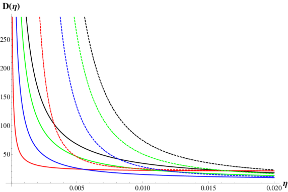
Figure 1: Dynamical diffusion as a function of disorder for different values of $\omega$ in arbitrary units. From red to black solid lines, $\omega$ increase. Dashed lines for dynamical diffusion at order $O(\hbar^{2})$.

$$-\frac{4v_{F}n_{F}}{i\omega}\frac{dv_{F}}{d\Lambda}+\frac{i\omega}{\pi\eta}\ln(a\Lambda)=0$$ (105)

and the solution reads

$$v_{F}(\Lambda)=\sqrt{v_{F_{0}}^{2}-\frac{\omega^{2}}{2\pi\eta n_{F}}\ln(\Lambda)}$$ (106)

because we are in the approximation $\omega\rightarrow 0$, last equation reads

$$v_{F}(\Lambda)=v_{F_{0}}-\frac{\omega^{2}}{4\pi n_{F}\eta v_{F}^{(0)}}\ln(\Lambda)$$ (107)

which is similar to the results found in ([41], [42]) and shows a singular behavior with the impurity factor $\eta$ that is similar to the singular behavior of the Fermi velocity with impurities found in [43]. Using eq.(106), the dynamical diffusion at order $\hbar^{0}$ reads

$$D(\omega)=\frac{iv_{F_{0}}^{2}}{\omega}+\frac{i\omega}{2\pi\eta n_{F}}\ln(a)$$ (108)

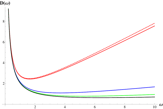
Figure 2: Dynamical diffusion as a function of $\omega$ for different values of $\eta$ in arbitrary units. From red to black solid lines, $\eta$ increase. Dashed lines for dynamical diffusion at order $O(\hbar^{2})$.

From last equation, there is no real value for $\omega$ where $D(\omega)=0$, which is expected because suppression of diffusion can be achieved by taking into account maximally crossed diagrams in the perturbation expansion. Nevertheless, we can plot $D(\omega,\eta)$ as a function of $\omega$ for different values of $\eta$ and $D(\omega,\eta)$ as a function of $\eta$ for different values of $\omega$. Both figures show the diffusion pole at $\omega=0$  (see 1 and 2). Dynamical diffusion tends to $\frac{v_{F_{0}}^{2}}{2i\omega}$ for $\eta\rightarrow\infty$. In turn, dynamical diffusion shows a minimum which corresponds to the following frequency

$$\omega=\sqrt{\frac{2\pi v_{F_{0}}^{2}\eta n_{F}}{\ln(a)}}$$ (109)

which is proportional to the impurity potential $V_{0}$. This implies that at low resonance frequencies, a decrease in the diffusion can be expected. The full renormalization group equation can be computed in the no-disorder limit $\eta\rightarrow 0$, which gives the following differential equation at order $O(\hbar^{j})$:

$$\frac{dv_{F}}{v_{F}}=\frac{\Lambda^{j-1}d\Lambda}{(\frac{1}{a^{j}}-\Lambda^{j})}$$ (110)

where the solution reads

$$v_{F}(\Lambda)=v_{F_{0}}(\frac{1-a^{-j}}{\Lambda^{j}-a^{-j}})^{1/j}$$ (111)

In the cut off limit $\Lambda\rightarrow 0$, the Fermi velocity change as

$$\frac{v_{F}}{v_{F_{0}}}=a(a^{-j}-1)^{1/j}$$ (112)

which decreases with increasing order of $\hbar$. In turn, Fermi velocity at higher orders of $\hbar$ and in the no disorder limit do not depends on the frequency of the external perturbation. High impurity concentrations in graphene can lead to a diffusion suppresion which would leave without effect the high performance of the material sample as a gas sensor. Weak localization of electrons in doped graphene implies to take into account higher orders in the diagrammatic perturbation expansion of the current response function. Some theoretical computations has been done (see [44], [45]). For conventional impurities, the correction becomes positive and it leads to the fact that anti-localization is realized, which would enhance the gas sensor peformance. In contrast, negative corrections for short-range impurities are expected from symmetry consideration. This suggest that the high sensitivity of graphene to detect individual dopants is highly dependent on the quantum corrections to the conductivity. Finally, taking into account the first quantum correction to the renormalization group equation for $v_{F}$ we obtain

$$v_{F}dv_{F}=\frac{5\omega\hbar^{2}v_{F}^{2}}{3\pi\eta^{3}}\frac{d\Lambda}{L(\Lambda,\omega,\eta,a)}-\frac{1}{\pi\eta}\frac{d\Lambda}{\Lambda^{2}L(\Lambda,\omega,\eta,a)}$$ (113)

where

$$L(\Lambda,\omega,\eta,a)=\frac{1}{\Lambda}\left(\frac{4n_{F}}{\omega^{2}}+\frac{5}{3\pi}\frac{\hbar^{2}}{\eta^{3}}(\frac{1}{a^{2}}-\Lambda^{2})\right)$$ (114)

Solution of eq.(114) in a integral form reads

$$v_{F}^{2}(\Lambda)=v_{F_{0}}^{2}-\frac{2}{\pi\eta}\int_{1}^{\Lambda}\frac{d\Lambda^{\prime}}{\Lambda^{\prime 2}L(\Lambda^{\prime},\omega,\eta,a)}+\frac{10\omega\hbar^{2}}{3\pi\eta^{3}}\int_{1}^{\Lambda}\frac{v_{F}^{2}(\Lambda^{\prime})d\Lambda^{\prime}}{L(\Lambda^{\prime},\omega,\eta,a)}$$ (115)

at order $O(\hbar^{2})$ we need to compute the second term of r.h.s. of last equation

$$\int_{1}^{\Lambda}\frac{d\Lambda^{\prime}}{\Lambda^{\prime 2}L(\Lambda^{\prime},\omega,\eta,a)}=\frac{3a^{2}\pi\omega^{2}\eta^{3}}{10\hbar^{2}\omega^{2}+24a^{2}n_{F}\pi\eta^{3}}\ln\left[\frac{\left(5\hbar^{2}\omega^{2}(a^{2}-1)-12a^{2}n_{F}\pi\eta^{3}\right)\Lambda^{2}}{5\hbar^{2}\omega^{2}(a^{2}\Lambda^{2}-1)-12a^{2}n_{F}\pi\eta^{3}}\right]$$ (116)

Introducing $v_{F}^{2}(\Lambda)$ in eq.(115) inside the integral of the r.h.s. in the same equation and using eq.(116), the dynamical diffusion reads at order $O(\hbar^{2})$

$$D(\omega)=\frac{v_{F_{0}}^{2}}{\omega}+\frac{i\omega\ln(a)}{2\pi\eta n_{F}}+\frac{5\omega}{12\pi}\frac{v_{F_{0}}^{2}\hbar^{2}}{\eta^{3}n_{F}a^{2}}$$ (117)

The correction introduced at order $O(\hbar^{2})$ can be seen in both figures as dashed lines. In the case of dynamical diffusion in terms of frequency, the correction is small and only is appreciable for low values of $\eta$. In this sense, quantum corrections to the diffusion do not alter the behavior under local perturbations at linear order in $\omega$.

7 Conclusion

In this work a generalization of linear response theory with Kubo formula has been introduced for linear dispersion relations and spinor wave functions. A minimal conductivity can be found in the no disorder limit and the result is in discordance by a factor of $2$ with other theoretical results, although there is no consensus of the physical reason of such value. Using the generalization introduced in the first sections, an exact relation between current and density response functions can be obtained. Combining this result with the relation obtained with the continuity equation, an exact functional form of response functions are obtained, where in particular, a singular behavior appears at $\omega\rightarrow 0$ and $q\rightarrow 0$ limit. Finally, dynamical diffusion is computed through the relaxation function at low order in $\omega$. A regularization is introduced to avoid infrared divergences, which introduce a renormalization group equation for the Fermi velocity. Different contributions to this equation can be analyzed at different order in $\hbar$. Different results are obtained which are of importance for local pertubations of graphene sample.

8 Acknowledgment

This paper was partially supported by grants of CONICET (Argentina National Research Council) and Universidad Nacional del Sur (UNS) and by ANPCyT through PICT 1770, and PIP-CONICET Nos. 114-200901-00272 and 114-200901-00068 research grants, as well as by SGCyT-UNS., E.A.G. and P.V.J. are members of CONICET. P.B. and J. S.A. are fellow researchers at this institution.

The authors are extremely grateful to the referee, whose relevant observations have greatly improved the final version of this paper.

9 Appendix

9.1 Spectral weight

The Green function for Dirac fermion systems reads

$$G_{ij}^{R(A)}(\mathbf{r},\mathbf{r}^{\prime},E)=\int\frac{d^{2}\mathbf{k}}{(2\pi)^{2}}\frac{\psi_{i}^{(k)}(\mathbf{r})\psi_{j}^{(k){\dagger}}(\mathbf{r}^{\prime})}{E-v_{f}\hbar k(\mp)is}$$ (118)

we can define the spectral weight as

$$A_{ij}(\mathbf{r},\mathbf{r}^{\prime},E)=i[G_{ij}^{R}(\mathbf{r},\mathbf{r}^{\prime},E)-G_{ij}^{A}(\mathbf{r},\mathbf{r}^{\prime},E)]$$ (119)

If we integrate the spectral weight in the volume we obtain the density of states

$$\int d^{2}\mathbf{r}A_{ij}(\mathbf{r},\mathbf{r},E)=2\pi\delta_{ij}\int\frac{d^{2}\mathbf{k}}{(2\pi)^{2}}\delta(E-v_{f}\hbar k)=2\pi n(E)\delta_{ij}$$ (120)

where $n(E)$ is the density of states.

9.2 Electron-electron correlation function

The electron-electron hole correlation function reads

$$\Phi_{liil}^{RR}(E,E,\mathbf{q})=\int_{0}^{1/a}\int_{0}^{2\pi}\frac{dkkd\lambda}{(2\pi)^{2}}\varrho(\mathbf{k},\mathbf{q},E)$$ (121)

where $\varrho(\mathbf{k},\mathbf{q},E)=g_{R}(\left|\mathbf{k}+\mathbf{q}\right|,E)g_{R}(\left|\mathbf{k}-\mathbf{q}\right|,E)\alpha(\mathbf{k},\mathbf{q})$

$$g_{R}(\left|\mathbf{k}\pm\mathbf{q}\right|,E)=\frac{1}{E-\hbar v_{F}\left|\mathbf{k}\pm\mathbf{q}\right|-i\eta}$$ (122)

and

$$\alpha(\mathbf{k},\mathbf{q})=1+\frac{k^{2}-q^{2}}{\left|\mathbf{k}+\mathbf{q}\right|\left|\mathbf{k}-\mathbf{q}\right|}$$ (123)

We can take the $q$ derivate inside the integral in $k$. Taking into account that

$$\frac{\partial g_{R}(\left|\mathbf{k}\pm\mathbf{q}\right|,E)}{\partial\mathbf{q}}=-\frac{\hbar v_{F}\frac{\partial\left|\mathbf{k}\pm\mathbf{q}\right|}{\partial\mathbf{q}}}{(E-\hbar v_{F}\left|\mathbf{k}\pm\mathbf{q}\right|-i\eta)^{2}}=-\hbar v_{F}\frac{\partial\left|\mathbf{k}\pm\mathbf{q}\right|}{\partial\mathbf{q}}g_{R}^{2}(\left|\mathbf{k}\pm\mathbf{q}\right|,E)$$ (124)

then

$$\frac{\partial\varrho(\mathbf{k},\mathbf{q},E)}{\partial\mathbf{q}}=\varrho(\mathbf{k},\mathbf{q},E)B(\mathbf{k},\mathbf{q},E)$$ (125)

where

$$B(\mathbf{k},\mathbf{q},E)=-\hbar v_{F}\frac{\partial\left|\mathbf{k}+\mathbf{q}\right|}{\partial\mathbf{q}}g_{R}(\left|\mathbf{k}+\mathbf{q}\right|,E)-\hbar v_{F}\frac{\partial\left|\mathbf{k}-\mathbf{q}\right|}{\partial\mathbf{q}}g_{R}(\left|\mathbf{k}-\mathbf{q}\right|,E)+\frac{\partial\alpha(\mathbf{k},\mathbf{q})}{\partial\mathbf{q}}\frac{1}{\alpha(\mathbf{k},\mathbf{q})}$$ (126)

The second derivate reads

$$\frac{\partial^{2}\varrho(\mathbf{k},\mathbf{q},E)}{\partial\mathbf{q}^{2}}=\varrho(\mathbf{k},\mathbf{q},E)\left[B^{2}(\mathbf{k},\mathbf{q},E)+\frac{\partial B(\mathbf{k},\mathbf{q},E)}{\partial\mathbf{q}}\right]$$ (127)

where

$$\frac{\partial B(\mathbf{k},\mathbf{q},E)}{\partial\mathbf{q}}=g_{R}(\left|\mathbf{k}+\mathbf{q}\right|,E)\left[-\hbar v_{F}\frac{\partial^{2}\left|\mathbf{k}+\mathbf{q}\right|}{\partial\mathbf{q}^{2}}+\hbar^{2}v_{F}^{2}\left(\frac{\partial\left|\mathbf{k}+\mathbf{q}\right|}{\partial\mathbf{q}}\right)^{2}g_{R}(\left|\mathbf{k}+\mathbf{q}\right|,E)\right]+$$ (128)

$$g_{R}(\left|\mathbf{k}-\mathbf{q}\right|,E)\left[-\hbar v_{F}\frac{\partial^{2}\left|\mathbf{k}-\mathbf{q}\right|}{\partial\mathbf{q}^{2}}+\hbar^{2}v_{F}^{2}\left(\frac{\partial\left|\mathbf{k}-\mathbf{q}\right|}{\partial\mathbf{q}}\right)^{2}g_{R}(\left|\mathbf{k}-\mathbf{q}\right|,E)\right]+$$

$$\frac{1}{\alpha(\mathbf{k},\mathbf{q})}\left[\frac{\partial^{2}\alpha(\mathbf{k},\mathbf{q})}{\partial\mathbf{q}^{2}}-\frac{1}{\alpha(\mathbf{k},\mathbf{q})}\left(\frac{\partial\alpha(\mathbf{k},\mathbf{q})}{\partial\mathbf{q}}\right)^{2}\right]$$

Finally using that

$$\frac{\partial\left|\mathbf{k}\pm\mathbf{q}\right|}{\partial\mathbf{q}}=\frac{q\pm k\cos\lambda}{\left|\mathbf{k}\pm\mathbf{q}\right|}$$ (129)

and that the second derivate reads

$$\frac{\partial^{2}\left|\mathbf{k}\pm\mathbf{q}\right|}{\partial\mathbf{q}^{2}}=\frac{1}{\left|\mathbf{k}\pm\mathbf{q}\right|}-\frac{(q\pm k\cos\lambda)^{2}}{\left|\mathbf{k}\pm\mathbf{q}\right|^{3}}$$ (130)

Putting $\mathbf{q}=0$ in eq.(127)

$$\varrho(k,0,E)=2g_{R}(\mathbf{k},E)g_{R}(\mathbf{k},E)$$ (131)

and using that $\frac{\partial\alpha(k,\mathbf{q})}{\partial\mathbf{q}}\mid_{\mathbf{q}=0}=0$,,

$$B^{2}(k,0,E)=0$$ (132)

In turn,

$$\frac{\partial B(\mathbf{k},\mathbf{q},E)}{\partial\mathbf{q}}=2g_{R}(\mathbf{k},E)\left[-\hbar v_{F}\frac{\sin^{2}\lambda}{k}+\hbar^{2}v_{F}^{2}\cos^{2}\lambda g_{R}(k,E)\right]-\frac{2\sin^{2}\lambda}{k^{2}}$$ (133)

where we have used that

$$\frac{\partial^{2}\alpha(\mathbf{k},\mathbf{q})}{\partial\mathbf{q}^{2}}\mid_{\mathbf{q}=0}=-\frac{4\sin^{2}\lambda}{k^{2}}$$ (134)

Finally the second derivate of $\varrho(\mathbf{k},\mathbf{q},E)$ at $\mathbf{q}=0$ reads

$$\frac{\partial^{2}\varrho(\mathbf{k},\mathbf{q},E)}{\partial\mathbf{q}^{2}}\mid_{\mathbf{q}=0}=4g_{R}^{2}(\mathbf{k},E)\left[g_{R}(\mathbf{k},E)\left[-\hbar v_{F}\frac{\sin^{2}\lambda}{k}+\hbar^{2}v_{F}^{2}\cos^{2}\lambda g_{R}(\mathbf{k},E)\right]-\frac{\sin^{2}\lambda}{k^{2}}\right]$$ (135)

which is the desired result which will be used in Section VI.

References

• [1] K. S. Novoselov, A. K. Geim, S. V. Morozov, D. Jiang, M. I. Katsnelson, I. V. Grigorieva, S. V. Dubonos and A. A. Firsov, Nature, 438, 197 (2005).
• [2] A.K. Geim and K. S. Novoselov, Nature Materials, 6, 183 (2007).
• [3] Y. B. Zhang, Y.W. Tan, H. L. Stormer and P. Kim, Nature, 438, 201 (2005).
• [4] A. H. Castro Neto, F. Guinea, N. M. R. Peres, K. S. Novoselov and A. K. Geim, Rev. Mod. Phys., 81, 109 (2009).
• [5] M. O. Goerbig, Rev. Mod. Phys., 83, 4 (2011).
• [6] J. McClure, Phys. Rev., 104, 666 (1956).
• [7] V. P. Gusynin and S. G. Sharapov, Phys. Rev. Lett., 95, 146801 (2005).
• [8] A. H. Castro Neto, F. Guinea and N. M. R. Peres, Phys. Rev. B, 73, 205408 (2006).
• [9] K. Ziegler, Phys. Rev. B, 75, 233407, (2007).
• [10] Y.V. Skrypnyk and V.M. Loktev, Phys. Rev. B, 82, 085436 (2010).
• [11] R. Kubo, Lectures in Theoretical Physics (Wiley-Interscience, New York, 1959).
• [12] V. Janis, J. Kolorenc and V. Spicka, Eur. Phys. J. B, 35, 77-91 (2003).
• [13] G.D. Mahan, Phys. Rev. B, 69, 125407 (2004).
• [14] E. Rotenberg, Graphene Nanoelectronics, edited by H. Raza (Springer-Verlag, Berlin, Heidelberg, 2012).
• [15] R. Ströbel, J. Garche, P. T. Moseley, L. Jörissen, G. Wolf, J. Pow. Sour., 159, 781-801 (2006).
• [16] J. Jiang, Q. Gao, Z. Zheng, K. Xia, J. Hu, Int. J. Hydrogen Energy, 35, 210-216 (2010).
• [17] M. Sankaran, B. Viswanathan, M. Srinivasa, Int. J. Hydrogen Energy, 33, 393-403 (2008).
• [18] H. Zeng, J. Zhao, J. W. Wei, H. F. Hu, Eur. Phys. J. B, 79, 335-340 (2011).
• [19] H. Y. Wu, X. Fan, J. L. Kuo, W. Q. Deng, J. Phys. Chem. C, 115, 9241-9249 (2011).
• [20] Y. C. Lin, C. Y. Lin, P. W. Chiu, Appl. Phys. Lett., 96, 133110-3 (2010).
• [21] D. H. Lee, J. A. Lee, W. J. Lee, S. O. Kim, Small, 7, 95-100 (2011).
• [22] P. A. Pandey, N. R. Wilson and J. A. Covington, Sensors and Actuators B: Chemical, 183, 478-487 (2013).
• [23] I. Lopez-Corral, E. German, A. Juan, M. A. Volpe and G. P. Brizuela, J. Phys. Chem. C, 115, 4315–4323 (2011).
• [24] B. D. Adams, C. K. Ostrom, S. Chen and A. Chen, J. Phys. Chem. C, 114, 19875-19882 (2010).
• [25] F. Schedin, A. K. Geim, S. V. Moeozov, E. W. Hill, P. Blake,  M. I. Katsnelson and K. S. Novoselov, Nat. Mater., 6, 652 (2007).
• [26] I. I. Barbolina, K. S. Novoselov, S. V. Morozov, S. V. Dubonos, M. Missous, A. O. Volkov, D. A. Christian, I. V. Grigorieva and A. K. Geim, Appl. Phys. Lett., 88, 013901 (2006).
• [27] J. Kong, N. R. Franklin, C. Zhou, M. G. Chapline, S. Peng, K. Cho and H. Dai, Science, 287, 622 (2000).
• [28] P. W. Anderson, Phys. Rev., 109, 1492 (1958).
• [29] J. Rammer, Quantum transport theory (Perseus books, Reading, Massachusetts, 1998).
• [30] N. M. R. Peres, F. Guinea and A. H. Castro Neto, Phys. Rev. B, 73, 125411 (2006).
• [31] V. Janis and J. Kolorenc, Mod. Phys. Lett. B, 18, 1051 (2004).
• [32] Y. Skrypnyk, Jour. Non-Crystalline Solids, 352, 4325–4330 (2006).
• [33] Y. Skrypnyk, Phys. Rev. B, 70, 212201 (2004).
• [34] V. M. Loktev and Y. G. Pogorelov, Low Temp. Phys. 27, 767 (2001).
• [35] V. M. Loktev and Y. G. Pogorelov, Nodal quasiparticles in doped d-wave superconductors: self-consistent T-matrix approach, arXiv:cond-mat/0308427.
• [36] A. F. Ioffe, and A. R. Regel, Prog. Semicond. 4, 237 (1960).
• [37] B. Velický, Phys. Rev., 184, 614 (1969).
• [38] G. Baym and L. P. Kadanoff, Phys. Rev. 124, 287 (1961).
• [39] G. Baym. Phys. Rev. 127,1391 (1962).
• [40] D. Belitz and T. R. Kirkpatrick. The Anderson-Mott transition. Rev. Mod. Phys. 66, 261 (1994).
• [41] C. Attaccalite and A. Rubio, Phys. Status Solidi B, 246, 11–12, 2523–2526 (2009).
• [42] H. Pei-Song, O. Sung-Jin, C. Yu and T. Guang-Shan, Commun. Theor. Phys., 54, 897–907 (2010).
• [43] Yu. V. Skrypnyk and V. M. Loktev, JETP. Letters, 94, 7, 565–569 (2011).
• [44] M. O. Nestoklon, N. S. Averkiev and S. A. Tarasenko, Solid State Comm., 151, 1550 (2011).
• [45] H. Suzuura and T. Ando, J. Phys Soc. Jpn., 72, Suppl. A, pp. 69–70 (2003).