BICEP’s bispectrum

Abstract

The simplest interpretation of the Bicep2 result is that the scalar primordial power spectrum is slightly suppressed at large scales Contaldi et al. (2014); Contaldi (2014). These models result in a large tensor-to-scalar ratio $r$. In this work we show that the type of inflationary trajectory favoured by Bicep2 also leads to a larger non-Gaussian signal at large scales, roughly an order of magnitude larger than a standard slow-roll trajectory.

I Introduction

The recent results from Bicep2 Ade et al. (2014), hinting at a detection of primordial $B$-mode power in the Cosmic Microwave Background (CMB) polarisation, place the inflationary paradigm on much firmer footing. This result, in combination with the Planck total intensity measurement Ade et al. (2013), imply that primordial perturbations are generated from an almost de-Sitter like phase of expansion early in the Universe’s history before the standard big bang scenario.

At first glance there is potential tension between the polarisation measurements made by Bicep2 and Planck’s total intensity measurements. Planck’s power spectrum is lower than the best-fit $\Lambda$CDM models at multipoles $\ell\lesssim 40$ and Bicep2’s high $B$-mode measurement exacerbates this since tensor modes also contribute to the total intensity. The tension is indicated by the difference in the $r\sim 0.2$ value implied by Bicep2’s measurements and the 95% limit of $r<0.1$ implied by the Planck data for $\Lambda$CDM models. Many authors have pointed out how the tension can be alleviated by going beyond the primordial power-law, $\Lambda$CDM paradigm by allowing running of the spectral indices, enhanced neutrino contributions (see for examples Czerny et al. (2014); Contaldi et al. (2014); Gong and Gong (2014); Zhang et al. (2014)) or more exotic scenarios Anchordoqui et al. (2014). However the simplest explanation, that also fits the data best, is one where there is a slight change in acceleration trajectory during the inflationary phase when the largest modes were exiting the horizon. This was shown by Contaldi et al. (2014) where a specific model was used to generate a slightly faster rolling trajectory at early times. The effect of such a “slow-to-slow-roll” transition is to result in a slightly suppressed primordial, scalar power spectrum that fits the Planck data despite the large tensor contribution required by Bicep2. In Contaldi (2014) the author analyses generalised accelerating, or inflating, trajectories that fit the combination of Bicep2 and Planck data and conclude that the suppression is required at a significant level and the best-fit trajectories are all of the form where the acceleration has a slight enhancement at early times.

An alternative explanation is that the $B$-mode power observed by Bicep2 is not due to foregrounds and is not primordial. This possibility has been discussed by various authors Mortonson and Seljak (2014); Flauger et al. (2014) who point out that more measurements on the frequency dependence of the signal are required to definitively state whether we have detected the signature of primordial tensor modes. These measurements will be provided in part by the Planck polarisation analysis and Bicep2’s cross-correlation with further KECK data Ade et al. (2014).

If the Bicep2 result stands the test of time then the signal we point out in the analysis below is expected to be present if the simplest models of inflation driven by a single, slow-rolling scalar field are the explanation behind the measurements. In this case a measurement of tensor mode amplitude, or $r$, is a direct measurement of the background acceleration since $r\sim 16\epsilon$ and the tension between Bicep2 polarisation and Planck total intensity measurements implies a change in the acceleration at early times. In turn, the change in acceleration enhances the non-Gaussianity on scales that were exiting the horizon while the acceleration was changing.

In this paper we construct a simple toy-model inspired by the best fitting trajectories found in Contaldi (2014) and calculate its bispectrum numerically. At small scales, as one would expect, the non-Gaussianity is small $\mathcal{O}(10^{-2})$ Maldacena (2003); Creminelli and Zaldarriaga (2004) but at large scales, where the scalar power spectrum is suppressed, the non-Gaussianity can be significantly larger, $\mathcal{O}(10^{-1})$. The results are compared against the slow-roll approximation in the equilateral configuration and the squeezed limit consistency relation. Whilst at small scales there is exceptional agreement with the slow-roll approximation, at large scales the results can deviate by up to 10%.

This paper is organised as follows. We outline the calculation of the scalar and tensor power spectra in Section II and summarise the calculation of the bispectrum in Section III. Our results are presented in Section IV and we discuss their implications in Section V.

II Computation of the scalar power spectrum

The calculation is best performed in a gauge where all the scalar perturbations are absorbed into the metric such that $g_{ij}=a^{2}\,(t)e^{2\zeta(t,\mathbf{x})}\delta_{ij}$ and the inflaton perturbation $\delta\phi(t,\mathbf{x})=0$. The primordial power spectrum is then simply given by:

$$\langle\zeta_{k_{1}}\zeta^{\star}_{k_{2}}\rangle=(2\pi)^{3}\delta^{(3)}(\mathbf{k}_{1}+\mathbf{k}_{2})P_{\zeta}(k_{1})\,,$$ (1)

where $\mathbf{k}$ is the Fourier wavevector and $k\equiv|\mathbf{k}|$. The mode $\zeta_{k}(t)$ satisfies the Mukhanov-Sasaki equation Mukhanov (1985); Sasaki (1986)

$$\frac{\mathrm{d}^{2}\zeta_{k}}{\mathrm{d}N^{2}}+(3+\epsilon-2\eta)\frac{\mathrm{d}\zeta_{k}}{\mathrm{d}N}+\frac{k^{2}}{a^{2}H^{2}}\zeta_{k}=0\,.$$ (2)

In the above $N$ is the number of $e-$folds which increases with time or alternatively

$$H=\frac{\dot{a}}{a}=\frac{dN}{dt}\,,$$ (3)

and $\epsilon$ and $\eta$ are the usual slow-roll variables defined by

$$\epsilon=-\frac{\dot{H}}{H^{2}},\,\,\,\,\,\,\,\,\eta=\epsilon-\frac{1}{2H}\frac{d\ln\epsilon}{dt}\,.$$ (4)

Outside the horizon $\zeta_{k}$ quickly goes to a constant and the power spectrum is then related to the freeze-out value of $\zeta_{k}$ on scales $k\ll aH$

$$P_{\zeta}(k)=\left|\zeta_{k\ll aH}\right|^{2}\,.$$ (5)

The initial conditions for the solutions to (2) can be set when the mode is much smaller than the horizon $k\gg aH$ and takes on the Bunch-Davies form Bunch and Davies (1978)

$$\zeta_{k}\to\frac{1}{M_{\rm pl}}\,\frac{e^{-ik\tau}}{2a\sqrt{k\epsilon}}\,,$$ (6)

where $\tau$ is conformal time defined by $\mathrm{d}N/\mathrm{d}\tau=aH$.

An identical calculation can be performed for the tensor power spectrum $P_{h}(k)=\left|h_{k\ll aH}\right|^{2}$ with $h_{k}$ satisfying the following differential equation

$$\frac{\mathrm{d}^{2}h_{k}}{\mathrm{d}N^{2}}+(3-\epsilon)\frac{\mathrm{d}h_{k}}{\mathrm{d}N}+\frac{k^{2}}{a^{2}H^{2}}h_{k}=0\,,$$ (7)

with initial condition

$$h_{k}\to\frac{1}{M_{\rm pl}}\,\frac{e^{-ik\tau}}{a\sqrt{2k}}\,,$$ (8)

in the limit where $k\gg aH$. Solving for $P_{\zeta}(k)$ and $P_{h}(k)$ numerically we can calculate $n_{s},r$ and $n_{t}$ directly from their definitions:

$$n_{s}(k_{\star}) = 1+\left.\frac{\mathrm{d}\ln\left[k^{3}P_{\zeta}(k)\right]}{\mathrm{d}\ln k}\right|_{k=k_{\star}}\,$$ (9)

$$r(k_{\star}) = 8\,\frac{P_{h}(k_{\star})}{P_{\zeta}(k_{\star})}\,$$

$$n_{t}(k_{\star}) = \left.\frac{\mathrm{d}\ln\left[k^{3}P_{h}(k)\right]}{\mathrm{d}\ln k}\right|_{k=k_{\star}}\,$$

The factor of 8 comes from how the tensor perturbations are normalised in the second order action.

The above procedure outlines the general calculation of the primordial power spectrum from inflation. In this work we are interested in specifying a background model favoured by the recent Bicep2 + Planck data. In particular we choose a function for $\epsilon$, then $\eta$ and $H$ are easily obtained by its derivative and integral respectively.

Instead of a direct function of time or $N$ though we specify $\epsilon(x)$ where $x=\ln(k^{\prime}/k_{\rm min})$. $k^{\prime}$ is the mode crossing the horizon at $e-$foldings $N$ ($k^{\prime}=aH$) and $k_{\rm min}\sim 10^{-5}(\text{Mpc})^{-1}$ is the largest scale observable today. In addition to being proportional to $r$ this condition allows one to easily specify how the background should evolve in our observational window. For concreteness we require $\epsilon$ to be relatively large, but still satisfying the slow-roll limit, at large scales and then to flatten out into another slow-roll regime with a smaller value. To this end we adopt a simple toy-model for $\epsilon$ as a function of x

$$\epsilon=\left\{\epsilon_{1}\tanh\left[(x-x_{0})\right]+\epsilon_{2}\right\}\left(1+mx\right)\,,$$ (10)

where the coefficients $\epsilon_{1}$, $\epsilon_{2}$, $m$, and $x_{0}$ are chosen to give a final power spectrum with the required suppression and position ($\sim 26\%$ and 1.5$\times 10^{-3}$ Mpc^-1 respectively Contaldi et al. (2014)) and $n_{s}\sim 0.96$ on small scales. Fig. 1 shows $\epsilon$ and $\eta$ as a function of $N$ for this toy-model and the resulting power spectra are shown in Fig. 2.

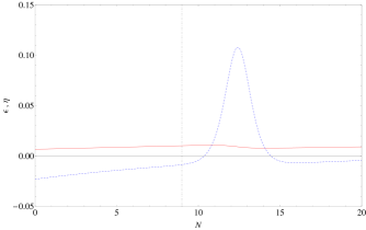
Figure 1: Background functions $\epsilon$ (red, solid) and $\eta$ (blue, dashed) of our toy-model plotted as a function of $e-$folds $N$. The grey vertical line indicates roughly the time when the first observable mode crosses the horizon.

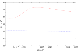
Figure 2: Left: Scalar (red, solid) and tensor (blue, dashed) dimensionless power-spectra. The tensors have been multiplied by a factor of 25 for comparison. Right: $r$ (red, solid) and $n_{s}-1$ as functions of $k$. The parameters in the toy-model were chosen to give a good match to the Planck and Bicep2 data.

III Computation of the bispectrum

The largest contribution to primordial non-Gaussianity will come from the bispectrum of the curvature perturbation

$$\langle\zeta_{k_{1}}\zeta_{k_{2}}\zeta_{k_{3}}\rangle=(2\pi)^{3}\delta^{(3)}(\mathbf{k}_{1}+\mathbf{k}_{2}+\mathbf{k}_{3})B(k_{1},k_{2},k_{3})\,.$$ (11)

The quantity that is often quoted in observational constraints is the dimensionless, reduced bispectrum

$$f_{\mathrm{NL}}(k_{1},k_{2},k_{3}) = \frac{5}{6}\,B(k_{1},k_{2},k_{3})/\left(|\zeta_{k_{1}}|^{2}|\zeta_{k_{2}}|^{2}+\right.$$ (12)

$$\left.|\zeta_{k_{1}}|^{2}|\zeta_{k_{3}}|^{2}+|\zeta_{k_{2}}|^{2}|\zeta_{k_{3}}|^{2}\right)\,,$$

The analytical calculation is much simpler if we consider the equilateral configuration $f_{\text{NL}}(k,k,k)$ however this is not a directly observed quantity as the estimator requires $B(k_{1},k_{2},k_{3})$ to be factorizable Creminelli et al. (2006). This is not true for the general case, which we are considering. However the overall amplitude of the reduced bispectrum gives a good indication of the size of the expected observable $f_{\mathrm{NL}}$.

All theories of inflation will produce a non-zero bispectrum. This is simply because gravity coupled to a scalar field is a non-linear theory and will contain interaction terms for the primordial curvature perturbation $\zeta(t,\textbf{x})$. These interaction terms will source the bispectrum with the largest contributors coming from tree-level diagrams associated with the cubic interaction terms. The bispectrum can then be calculated using the “in-in” formalism Adshead et al. (2009); Maldacena (2003); Seery and Lidsey (2005), which to tree level becomes

$$\langle\zeta^{3}(t)\rangle=-i\int_{-\infty}^{t}\mathrm{d}t^{\prime}\langle\left[\zeta^{3}(t),H_{\text{int}}(t^{\prime})\right]\rangle\,,$$ (13)

where $H_{\text{int}}$ is the interaction Hamiltonian associated with the following third order action

$$S_{3} = \!\!\int d^{4}x\,a^{3}\epsilon\left[\left(2\eta-\epsilon\right)\zeta\dot{\zeta}^{2}+\frac{1}{a^{2}}\epsilon\zeta(\partial\zeta)^{2}\right.$$ (14)

$$\!\!\!\!\left.-(\epsilon-\eta)\zeta^{2}\partial^{2}\zeta-2\epsilon\left(1-\frac{\epsilon}{4}\right)\dot{\zeta}\partial_{i}\zeta\partial_{i}\partial^{-2}\dot{\zeta}\right.$$

$$\!\!\!\!\left.+\frac{\epsilon^{2}}{4}\partial^{2}\zeta\partial_{i}\partial^{-2}\dot{\zeta}\partial_{i}\partial^{-2}\dot{\zeta}\right]\,,$$

The numerical calculation of the bispectrum is technically challenging and is described in more detail in Horner and Contaldi (2013). Briefly, for the equilateral configuration it requires the calculation of the following integral

$$f_{\mathrm{NL}}=\frac{1}{3|\zeta|^{4}}\times{\cal I}\left[\zeta^{*3}\int_{N_{0}}^{N_{1}}dN\,(f_{1}\zeta^{3}+f_{2}\zeta\zeta^{\prime 2})\right]\,,$$ (15)

where $\zeta=\zeta_{k}$, $\zeta^{\prime}=\mathrm{d}\zeta/\mathrm{d}N$, and $\cal I$ represents the imaginary part. The background functions $f_{i}$ are given by

$$\!\!\!\!\!f_{1} = \frac{5k^{2}a\epsilon}{H}(2\eta-3\epsilon)\,,$$

$$\!\!\!\!\!f_{2} = -5Ha^{3}\epsilon\left(4\eta-\frac{3}{4}\epsilon^{2}\right)\,.$$ (16)

The times $N_{0}$ and $N_{1}$ correspond to when the mode is sufficiently sub- and super-horizon respectively. For calculating the shape dependence we restrict ourselves to the case of isosceles triangles so we parametrise our modes in the following way. $|\textbf{k}_{1}|=|\textbf{k}_{2}|=k,|\textbf{k}_{3}|=\beta k$. This covers most configurations of interest ($\beta=0$ is squeezed, $\beta=1$ is equilateral, $\beta=2$ is folded) and is simple to interpret.

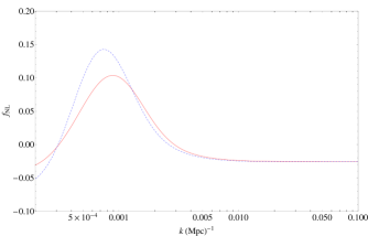
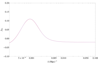
Figure 3: $f_{\rm NL}$as a function of $k$ for equilateral (left) and squeezed (right) configurations. The blue (dashed) curves represents the numerical calculation. The red curves represent the slow roll approximation (17) (left) and the consistency condition $5/12(n_{s}-1)$ (right). It is not possible to calculate the exact squeezed configuration numerically so a configuration with $\beta=0.1$ was used to approximate the squeezed limit.

IV Results

For the toy-model given in (10) the non-Gaussianity amplitude is plotted in Fig. 3. For comparison, as well as a consistency check, we plot the full-numerical calculation (blue-dashed) as well as the the slow-roll approximation (red-solid) which, in the equilateral limit, is given by Maldacena (2003)

$$f_{\mathrm{NL}}(k)=\frac{5}{12}\left(n_{s}(k)-1+\frac{5}{6}n_{t}(k)\right)\,.$$ (17)

In applying this formula we used the exact values of $n_{s}$ and $n_{t}$ given by equations 9. As can be seen from Fig. 3, if values close to $r\sim 0.2$ are confirmed from polarisation measurements, the non-Gaussianity on large scales are likely to be an order of magnitude larger than expected. This is simply because $r\propto\epsilon$ but on smaller scales $\epsilon$ is constrained to be lower by the total intensity measurements. The only way to reconcile the two regimes is by having $\epsilon$ change to a lower value at later times and this results in an enhancement of non-Gaussianity being generated as the value is changing. Fig. 3 also shows that, even with strong scale dependence, there is remarkable agreement between the full numerical results and the Maldacena formula, with deviations only occurring at the largest scales. Fig. 4 shows the complete scale and shape dependence of $f_{\rm NL}$.

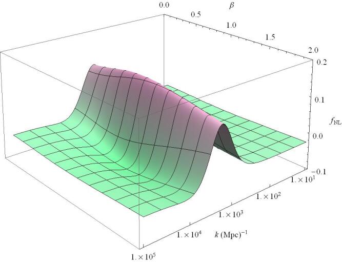
Figure 4: $f_{\rm NL}$as a function of scale $k$ and shape $\beta$. There is a mild peak in the equilateral limit, $\beta=1$. For all shapes the non-Gaussianity peaks around the scales corresponding to the size of the horizon at the time when the background acceleration is changing.

V Discussion

Models of inflation that contain a feature causing the background acceleration to change can reconcile Planck and Bicep2 observations of the CMB total intensity and polarisation power spectra. We have shown that these models result in enhanced non-Gaussianity at scales corresponding to the size of the horizon at the time when the acceleration is changing. The level of non-Gaussianity at these scales is an order of magnitude larger than what is expected in the standard case with no feature and is strongly scale dependent.

Whilst the effect was illustrated using a simple toy-model of the background evolution $H(t),\epsilon(t)$, etc, we expect the non-Gaussian enhancement to be present in any model where the acceleration changes relatively quickly in order to fit the Planck and Bicep2 combination. The exact form of non-Gaussianity will obviously be model dependent.

It is not clear that this level of non-Gaussianity will be observable since it corresponds to scales $\ell\sim 2\to 80$ where there may not be a sufficient number of CMB modes on the sky to ever constrain $f_{\rm NL}$to ${\cal O}(10^{-1})$. However cross-correlation with other surveys of large scale structure may help to constrain non-Gaussianity on these scales. In particular it may be possible to detect any anomalous correlation of modes induced by the non-Gaussianity.

The biggest question at this time however is whether or not the claimed detection of primordial tensor modes by Bicep2 is correct. This will be addressed in the near future as the polarisation signal is observed at more frequencies at the same signal-to-noise levels reached by the Bicep2 experiment.