Overstability of acoustic waves in strongly magnetized anisotropic MHD shear flows

Abstract

We present a linear stability analysis of the perturbation modes in anisotropic MHD flows with velocity shear and strong magnetic field. Collisionless or weakly collisional plasma is described within the 16-momentum MHD fluid closure model, that takes into account not only the effect of pressure anisotropy, but also the effect of anisotropic heat fluxes. In this model the low frequency acoustic wave is revealed into a standard acoustic mode and higher frequency fast thermo-acoustic and lower frequency slow thermo-acoustic waves. It is shown that thermo-acoustic waves become unstable and grow exponentially when the heat flux parameter exceeds some critical value. It seems that velocity shear makes thermo-acoustic waves overstable even at subcritical heat flux parameters. Thus, when the effect of heat fluxes is not profound acoustic waves will grow due to the velocity shear, while at supercritical heat fluxes the flow reveals compressible thermal instability. Anisotropic thermal instability should be also important in astrophysical environments, where it will limit the maximal value of magnetic field that a low density ionized anisotropic flow can sustain.

I Introduction

Physical properties of space plasmas in magnetized environments often reveal their collisioness or weakly collisional character. Among these are the magnetosphere of the Earth and other planets, solar and stellar winds, astrophysical jets, magnetized accretion around compact objects, as well as ionized low density interstellar and intercluster media. Such plasmas can not be described by the simple one fluid magnetohydrodynamic (MHD) approach, since they are characterized by pressure and temperature anisotropies with respect to the magnetic field orientation.

Observations show strong anisotropy of solar wind plasmas OMHC12 ; HWC12 . Similar features are observed in the near earth magnetospheric plasmas. In this case, the mean free path is longer than the gyroradius of the particle, and thus MHD description is not adequate. Similar features should occur in the inner regions of accretion disks around black holes, where the typical collision distance is longer then the event horizon of the central black hole. In such situations, the magnetorotational instability that is thought to drive accretion should be considered in the collisionless limit Mikh08a ; Mikh08b ; QDH02 ; SQHS07 ; SQHS03 . It has been also shown that pressure anisotropy has a significant effect on MHD turbulence in the intracluster medium SdKFLN12 ; NdKS12 ; MS14 .

The most commonly used approach to analyze the anisotropic effects in the one fluid approximation is the Chew-Goldberger-Low (CGL) approximation CGL56 . This limit is often referred to as double adiabatic law MHD, emphasizing the adiabatic equations of state that are the parallel and perpendicular components of the pressure, respectively.

The CGL closure of the MHD equations does not include the effects of heat fluxes on the flow. This in turn sets a high frequency limit to the applicability of the model. Indeed, heat fluxes can be neglected for processes with characteristic frequencies much higher than thermal buoyancy effects. Hence, it can be marginally valid for the stability analysis, where modes with zero or imaginary frequencies are involved. Indeed, the CGL model was only a partial success when describing well known instabilities in collisionless plasmas: the fire-hose and mirror instabilities. Although the double adiabatic anisotropic description was able to resolve these instabilities, the criteria of their onset were not properly replicated as compared to the results of a more rigorous kinetic theory. As a matter of fact, results of the CGL model, especially on the flow stability analysis, should be considered in some sense as a somewhat crude estimate of the flow stability. The deficiencies of the CGL model in the stability analysis of anisotropic plasmas are already well known. Attempts have been made to overcome them using linearized kinetic equations for the parallel and transverse components of the pressure. The stability of low frequency modes in this approach is studied based on the variational principle for the potential energy Grigorev07 ; Grigorev08 .

Still, probably the most effective method to overcome the deficiencies of the CGL closure method in the MHD approximation is to consider three additional moments during the closure method Oraevskii68 . In this limit, the authors retain the heat fluxes along the magnetic field and derive a so-called 16-momentum approximation of anisotropic MHD plasmas Dzhalilov08 ; Kuznetsov09 ; Kuznetsov10 ; Dzhalilov10 ; Ramos03 . Indeed, the 16-momentum anisotropic MHD model proved to be successful in replicating properties of classical instabilities (mirror, fire-hose) obtained in kinetic theory using the fluid approximation Dzhalilov10 ; Kuznetsov09 . The 16-momentum MHD approximation has been used to describe the instability of entropy waves in cosmic plasma Somov08 , or to propose a solar coronal heating mechanism due to large scale wave mechanism Dzhalilov11 .

The purpose of the present paper is to analyze the linear stability of weakly collisional plasmas in the presence of inhomogeneous background flow. Indeed, velocity shear is a widely occurring factor in solar and stellar winds and accretion flows. An attempt to describe the velocity shear effects in the CGL-MHD approximation has shown a diversity of velocity shear effects occurring in pressure anisotropic flows. Modifications to the fire-hose and mirror instabilities have been analyzed Chagelishvili97 . Still, the obtained results are to be considered within the limitations of the CGL model.

In the present paper we adopt a simple shear configuration with a flow aligned with the magnetic field, and a shear normal to the magnetic field direction. We present the results of linear analysis of perturbation modes in an anisotropic MHD shear flow in the strong magnetic field limit. In the context of flow stability we focus on the low frequency solutions of the dispersion equation. It seems that the existence of anisotropic heat fluxes modifies the linear spectrum of the system. Stationary entropy modes become compressional and we identify the fast and slow thermo-acoustic modes in the linear spectrum. Hence, we study the stability of thermo-acoustic waves in shear flows.

The mathematical formalism of the physical model is described in Sec. 2. Here, we describe strongly magnetized anisotropic shear flow and introduce linear perturbations. Sec. 3 discusses the linear spectrum of the problem in the uniform and nonuniform flow limits. We study the linear spectrum and instabilities occurring for different heat flux parameters. The results are summarized in Sec. 4.

II Anisotropic MHD formalism

In this section we formulate the 16-momentum MHD framework Oraevskii68 ; Dzhalilov08 in order to study the linear stability of compressible plasmas with anisotropic pressure and heat fluxes. The standard MHD equations are complemented by anisotropic pressure terms as follows:

$${\mathrm{d}\rho\over\mathrm{d}t}+\rho(\nabla\cdot\mathbf{V})=0~{},$$ (1)

$$\rho{\mathrm{d}\mathbf{V}\over\mathrm{d}t}+\nabla\left(P_{\perp}+{B^{2}\over 8\pi}\right)-{1\over 4\pi}(\mathbf{B}\cdot\nabla)\mathbf{B}=\hskip 85.35826pt$$

$$~{}~{}~{}~{}=(P_{\perp}-P_{\|})\left[\mathbf{h}(\nabla\cdot\mathbf{h})+(\mathbf{h}\cdot\nabla)\mathbf{h}\right]+\mathbf{h}(\mathbf{h}\cdot\nabla)(P_{\perp}-P_{\|})~{},$$ (2)

$${\mathrm{d}\mathbf{B}\over\mathrm{d}t}+\mathbf{B}(\nabla\cdot\mathbf{V})-(\mathbf{B}\cdot\nabla)\mathbf{V}=0~{},$$ (3)

$$(\nabla\cdot\mathbf{B})=0~{}.$$ (4)

Here, for the shortness of notations we use the convective derivative $\mathrm{d}/\mathrm{d}t\equiv\partial/\partial t+(\mathbf{V}\cdot\nabla)$, and $\mathbf{h}=\mathbf{B}/B$ is the unity vector field following the streamlines of the magnetic field. Parallel and perpendicular pressure ($P_{\|}$,$P_{\perp}$) form two adiabatic invariants in the CGL model. However, in the 16-momentum approximation the derivatives of these CGL invariants are not zero due to the existence of nonzero heat fluxes ($S_{\|}$,$S_{\perp}$):

$${\mathrm{d}\over\mathrm{d}t}\left({P_{\|}B^{2}\over\rho^{3}}\right)=-{B^{2}\over\rho^{3}}\left[B(\mathbf{h}\cdot\nabla){S_{\|}\over B}+{2S_{\perp}\over B}(\mathbf{h}\cdot\nabla)B\right]~{},$$ (5)

$${\mathrm{d}\over\mathrm{d}t}\left({P_{\perp}\over\rho B}\right)=-{B\over\rho}(\mathbf{h}\cdot\nabla){S_{\perp}\over B^{2}}~{}.$$ (6)

Finally, the 16-momentum closure model provides two more equations for the heat fluxes:

$${\mathrm{d}\over\mathrm{d}t}\left({S_{\|}B^{3}\over\rho^{4}}\right)=-j{3P_{\|}B^{3}\over\rho^{4}}(\mathbf{h}\cdot\nabla){P_{\|}\over\rho}~{},$$ (7)

$${\mathrm{d}\over\mathrm{d}t}\left({S_{\perp}\over\rho^{2}}\right)=-j{P_{\|}\over\rho^{2}}\left[(\mathbf{h}\cdot\nabla){P_{\perp}\over\rho}+{P_{\perp}\over\rho}{P_{\perp}-P_{\|}\over P_{\|}B}(\mathbf{h}\cdot\nabla)B\right]~{}.$$ (8)

The parameter $j$ is used to switch to the CGL limit with zero heat fluxes:

$$j=\left\{\begin{array}[]{lll}1&~{}~{}\mathrm{when}&(S_{\perp}\not=0~{},S_{\|}\not=0)\\ 0&~{}~{}\mathrm{when}&(S_{\perp}=0~{},S_{\|}=0)\end{array}\right.~{},$$

making it possible to set $S_{\perp}=S_{\|}\not=0$ consistently in the Eqs. (7,8).

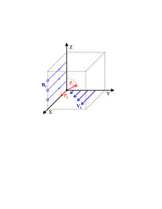
Figure 1: Equilibrium MHD configuration with shear flow along the background magnetic field. Direction parallel to the magnetic field is set by $X$ axis, while the perpendicular direction lays in the $YZ$ plane. The flow along the $X$ axis is nonuniform in the $Y$ direction.

II.1 Background Flow

We consider a stationary shear flow along the magnetic field with constant background density and temperature:

$$\mathbf{V_{0}}=(Ay,0,0)~{},~{}~{}\mathbf{B_{0}}=(B_{0},0,0)~{},$$ (9)

where $A$ is the velocity shear rate. Fig. 1 schematically shows the flow configuration.

We define an anisotropy parameter $\alpha$ as the ratio between the perpendicular and parallel components of the background pressure or heat fluxes:

$$\alpha\equiv{P_{\perp 0}/P_{\|0}}={S_{\perp 0}/S_{\|0}}~{}.$$ (10)

We may introduce sound speeds parallel and perpendicular to the background flow:

$$C_{\|}^{2}\equiv P_{\|0}/\rho_{0}~{},~{}~{}C_{\perp}^{2}\equiv P_{\perp 0}/\rho_{0}~{},$$ (11)

Hence we may define a non-dimensional anisotropic heat flux parameter as follows:

$$\gamma\equiv{S_{\|0}\over P_{\|0}C_{\|}}~{}.$$ (12)

The parameter $\gamma$ is the normalized measure of the heat flux effects in pressure anisotropic MHD flows. When the heat fluxes can be neglected ($j=0$, $\gamma=0$) we obtain the double adiabatic limit of the CGL anisotropic model.

II.2 Linear Perturbations

To proceed with a linear analysis of the anisotropic MHD shear flow we split the physical variables into background and perturbation components:

$${\bf\rho} = {\bf\rho_{0}}+{\bf\rho^{\prime}}~{},~{}~{}$$

$${\bf V} = {\bf V_{0}}+{\bf V^{\prime}}~{},$$

$${\bf B} = {\bf B_{0}}+{\bf B^{\prime}}~{},$$ (13)

$$P_{\parallel} = P_{0\parallel}+P_{\parallel}^{\prime}~{},~{}~{}~{}P_{\perp}=P_{0\perp}+P_{\perp}^{\prime}~{},$$

$$S_{\parallel} = S_{0\parallel}+S_{\parallel}^{\prime}~{},~{}~{}~{}S_{\perp}=S_{0\perp}+S_{\perp}^{\prime}~{}.$$

Hence, we may employ the shearing sheet formalism to analyze the linear dynamics of perturbations in shear flow Goldreich65 . In this limit the shearing transformation is used to transfer the spatial dependence due to the velocity shear into a temporal variation of the wave-numbers in the direction of the velocity shear and analyze the initial value problem. This method, often called a non-modal approach, is based on the study of the evolution of the spatial Fourier harmonics (SFH) in time Chagelishvili97 ; ChChLT97 ; T98 . Hence, we follow the non-modal analysis and introduce the spatial Fourier transformation with time dependent wave-numbers:

$$\Psi({\bf r},t)\propto\psi({\bf K},t)\exp\left({\rm i}K_{x}x+{\rm i}K_{y}(t)y+{\rm i}K_{z}z\right)~{},$$ (14)

where

$$K_{y}(t)=K_{y0}-AK_{x}t~{}.$$ (15)

Here $\Psi({\bf r},t)$ and $\psi({\bf K},t)$ are generalized vectors introduced for shortness of notations:

$$\Psi\equiv\left({\rho^{\prime}\over\rho_{0}},~{}{P_{\|}^{\prime}\over P_{\|0}},~{}{P_{\perp}^{\prime}\over P_{\perp 0}},~{}{S_{\|}^{\prime}\over P_{\|0}},~{}{S_{\perp}^{\prime}\over P_{\perp 0}},~{}{{\bf V^{\prime}}\over V_{A}},~{}{{\bf B^{\prime}}\over B_{0}}\right),$$ (16)

$$\psi\equiv\left({\rm i}{\varrho},~{}{\rm i}{p_{\|}},~{}{\rm i}{p_{\perp}},~{}{\rm i}{s_{\|}},~{}{\rm i}{s_{\perp}},~{}{\bf v},~{}{\rm i}{\bf b}\right)~{}.$$ (17)

Note that the perturbation SFH $\psi$ is introduced in the non-dimensional form with complex coefficients used to account for intrinsic phase differences between the kinetic and thermodynamic quantities in the wave-number space.

Linearized with respect to assumed to be small perturbations, the PDE system (1-8) can be transformed into a system of ODEs for the spatial harmonics of perturbations using the Fourier expansion (14). Hence, the system describing the evolution of linear perturbations in time will read as follows:

$$\dot{\varrho} = -k_{x}v_{x}-k_{y}v_{y}-k_{z}v_{z}$$ (18)

$$\dot{v}_{x} = -Rv_{y}+\beta_{\|}k_{x}p_{\|}+(\beta_{\perp}-\beta_{\|})k_{x}b_{x}$$ (19)

$$\dot{v}_{y} = \beta_{\perp}k_{y}p_{\perp}-(1+\beta_{\perp}-\beta_{\|})k_{x}b_{y}+k_{y}b_{x}$$ (20)

$$\dot{v_{z}} = \beta_{\perp}k_{z}p_{\perp}-(1+\beta_{\perp}-\beta_{\|})k_{x}b_{z}+k_{z}b_{x}$$ (21)

$$\dot{p_{\|}} = -3k_{x}v_{x}-k_{y}v_{y}-k_{z}v_{z}-ik_{x}s_{\|}+$$

$$~{}~{}~{}~{}~{}~{}~{}~{}~{}~{}~{}~{}~{}~{}~{}~{}~{}+{\rm i}\gamma(1-2\alpha^{2})\beta_{\|}^{1\over 2}k_{x}b_{x}-2{\rm}Rb_{y}~{},$$

$$\dot{p_{\perp}} = -k_{x}v_{x}-2k_{y}v_{y}-2k_{z}v_{z}-ik_{x}s_{\perp}+$$

$$~{}~{}~{}~{}~{}~{}~{}~{}~{}~{}~{}~{}~{}~{}~{}~{}~{}~{}~{}~{}~{}~{}~{}~{}~{}~{}~{}+2{\rm i}\gamma\beta_{\perp}^{1\over 2}k_{x}b_{x}+{\rm}Rb_{y}~{},$$

$$\dot{s_{\|}} = -4\gamma\beta_{\|}^{1\over 2}k_{x}v_{x}-\gamma\beta_{\|}^{1\over 2}k_{y}v_{y}-\gamma\beta_{\|}^{1\over 2}k_{z}v_{z}+$$

$$~{}~{}~{}~{}~{}~{}~{}~{}~{}~{}~{}~{}~{}~{}~{}~{}~{}+3{\rm i}j\beta_{\|}k_{x}\left(\rho-p_{\|}\right)-3\gamma R\beta_{\|}^{1\over 2}b_{y}~{},$$

$$\dot{s_{\perp}} = -2\gamma\beta_{\perp}^{1\over 2}k_{x}v_{x}-2\gamma\beta_{\perp}^{1\over 2}k_{y}v_{y}-2\gamma\beta_{\perp}^{1\over 2}k_{z}v_{z}+$$

$$~{}~{}~{}~{}~{}~{}~{}~{}~{}~{}~{}~{}~{}~{}~{}~{}~{}+{\rm i}j\beta_{\|}k_{x}\left(\rho-p_{\perp}+(1-\alpha)b_{x}\right)~{},$$

$$\dot{b_{y}} = k_{x}v_{y}$$ (26)

$$\dot{b_{z}} = k_{x}v_{z}$$ (27)

$$0 = k_{x}b_{x}+k_{y}b_{y}+k_{z}b_{z},$$ (28)

where $\textbf{k}\equiv\textbf{K}/K_{\perp}$ is non-dimensional wave-vector with $K_{\perp}=(K_{y}^{2}+K_{z}^{2})^{1\over 2}$, $\tau\equiv V_{A}K_{\perp}t$ is non-dimensional time, $\dot{\psi}$ denotes time derivative of $\psi$ with respect to $\tau$. We define longitudinal and transverse plasma $\beta$ parameters:

$$\beta_{\|}\equiv{C_{\|}^{2}\over V_{A}^{2}}~{},~{}~{}~{}\beta_{\perp}\equiv{C_{\perp}^{2}\over V_{A}^{2}}~{},$$

and $R\equiv A/(V_{A}K_{\perp})$ is the non-dimensional shear rate.

III Linear Spectrum

Strictly speaking, the linear spectrum of the problem can be obtained using the Fourier expansion of the spatial harmonics of the perturbations in time. In fact, the coefficients of the Eqs. (18-28) are explicitly time dependent due to the velocity shear of the flow. However, it is still possible to employ the adiabatic approximation when

$$\dot{\psi}({\rm k},\tau)\approx-{\rm i}\omega\psi({\rm k},\tau)~{},$$ (29)

where $\omega$ can be a slowly varying function in time. The considered approximation is valid for low or moderate velocity shear of the flow and is strongly justified for low frequency modes of the spectrum. The linear spectrum of anisotropic MHD uniform flow (with zero shear) is analyzed in Dzhalilov08 . Velocity shear introduces farther complications to the general dispersion equation (see Eqs. A1-A4 in the Appendix). In the present paper we intend to describe the compressible sound waves in more detail using the cold plasma approximation. In this limit the magnetic pressure dominates over the hydrodynamic one and hence:

$$\beta_{\|},\beta_{\perp}\ll 1~{}.$$ (30)

This leads to a somewhat simplified dispersion equation for the considered problem, that can be factorized into the high frequency

$$\omega^{2}-k_{x}^{2}=0$$ (31)

and low frequency modes:

$$(\omega^{2}-j\beta_{\|}k_{x}^{2})D_{0}-{\rm i}R\beta_{\perp}{k_{x}k_{y}\over k^{2}}D_{1}=0~{},$$ (32)

where

$$D_{0}=\omega^{4}-3(j+1)\beta_{\|}k_{x}^{2}\omega^{2}-4\gamma\beta_{\|}^{3\over 2}k_{x}^{3}\omega+3j\beta_{\|}^{2}k_{x}^{4}~{},~{}~{}~{}~{}$$ (33)

$$D_{1} = (2\omega^{5}+2\alpha\gamma\beta_{\|}^{1\over 2}k_{x}\omega^{4}-(5+7j)\beta_{\|}k_{x}^{2}\omega^{3}-~{}~{}~{}~{}~{}~{}~{}~{}$$ (34)

$$- (2\alpha(2+3j)+7)\gamma\beta_{\|}^{3\over 2}k_{x}^{3}\omega^{2}+$$

$$+ (j(3j+5)-6\alpha\gamma^{2})\beta_{\|}^{2}k_{x}^{4}\omega+$$

$$+ 3\gamma j\beta_{\|}^{5\over 2}k_{x}^{5})~{}.$$

We can solve the dispersion equation in the zero shear limit when it reduces to $(\omega^{2}-j\beta_{\|}k_{x}^{2})D_{0}=0$. In the absence of heat fluxes ($j=\gamma=0$), the dispersion relation reduces to $\omega^{2}(\omega^{2}-3\beta_{\|}k_{x}^{2})=0$ with the well known CGL solution for acoustic waves: $\omega^{2}=3\beta_{\|}k_{x}^{2}$. In case of nonzero heat fluxes we get three different periodic solutions:

• fast thermo-acoustic mode with $\omega_{+}=\beta_{\|}^{1\over 2}k_{x}\eta_{+}$,

• acoustic mode with $\omega_{s}^{2}=\beta_{\|}k_{x}^{2}$,

• slow thermo-acoustic mode with $\omega_{-}=\beta_{\|}^{1\over 2}k_{x}\eta_{-}$,

where $\eta_{\pm}$ are the upper and lower pair solutions of the equation: $\eta^{4}-6\eta^{2}-4\gamma\eta+3=0$. We identify these solutions as fast and slow thermo-acoustic modes since they obey the property: $\eta_{+}^{2}>1>\eta_{-}^{2}$. The linear instability for uniform flow with zero shear of velocity is found when heat flux parameter exceeds some critical value. Indeed, Fig. 2 shows the growth rate of the slow thermo-acoustic mode that becomes unstable at supercritical heat flux rates: $\gamma>\gamma_{cr}\approx 0.85$.

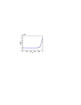
Figure 2: Growth rate of the compressible heat flux instability vs heat flux parameter $\gamma$ in the uniform flow: $R=0$. Figure reveals the critical value of heat flux parameter $\gamma_{cr}=0.85$ that is necessary for the instability.

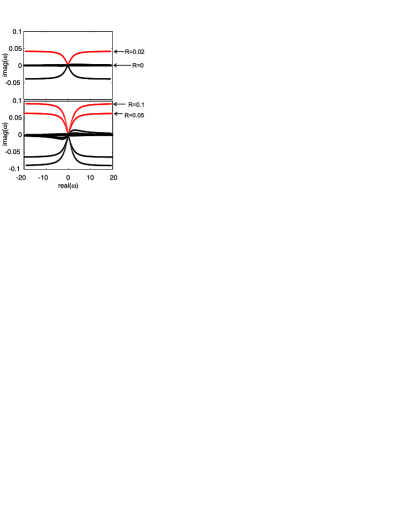
Figure 3: Dispersion curves at subcritical heat flux parameter $\gamma=0.5$, anisotropy parameter $\alpha=2$ and different values of normalized shear parameter: $R=0,0.02,0.05,0.1$. Here $\beta_{\|}=0.01$ and harmonics with $k_{y}/k_{x}=2$ are shown for different values of $k_{z}/k_{x}$. Instability growth rate grows with the velocity shear of the flow.

Figure 4: Dispersion curves at supercritical heat flux parameter $\gamma=1.5$, anisotropy parameter $\alpha=2$ and different values of normalized shear parameter: $R=0,0.02,0.05,0.1$. Here $\beta_{\|}=0.01$ and harmonics with $k_{y}/k_{x}=2$ are shown for different values of $k_{z}/k_{x}$. Effect of the velocity shear is dominated by the heat flux instability growth rate (see Fig. 5).

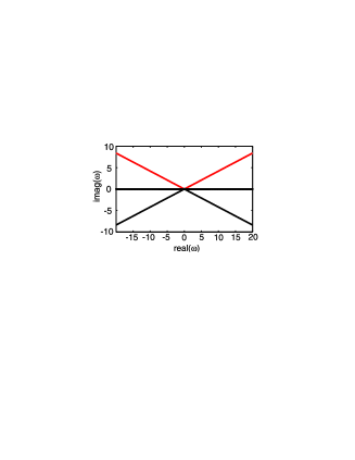
Figure 5: Dispersion curves at supercritical heat flux parameter $\gamma=1.5$ in zero shear limit: $R=0$. Figure shows that the growth rate of exponential thermal instability is much higher compared to the growth rate of acoustic overstability at the same parameters of the system (see Fig. 4).

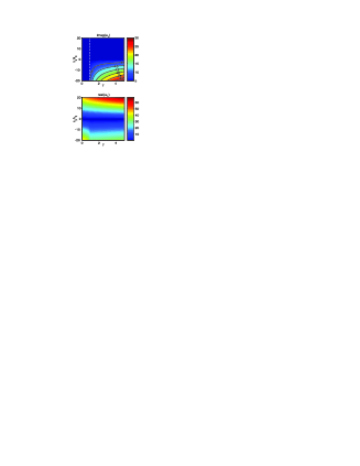
Figure 6: Surfaces of the growth rate ($Im(\omega)$) and frequency ($Re(\omega)$) of the fast thermo-acoustic mode are shown for the different values of stream-wise wave-number $k_{x}$ and heat flux parameter $\gamma$. Vertical white dashed lines shows the critical value of $\gamma$ parameter for the instability due to heat fluxes. Complex part reveals the instability area, where the real part of the solution is not vanishing. Moreover, in this area real part is similar to the complex one, thus identifying the overstability of the mode. The growth rates of the overstability increase with the growth of heat flux parameter and streamwise wavenumber.

III.1 Shear flow solutions

In the presence of velocity shear the linear modes are modified proportional to the transverse plasma beta $\beta_{\perp}$ and velocity shear rate $R$, see the second term in Eq. (32). For more specific results we use numerical methods to calculate the solutions of the dispersion equation.

Fig. 3 shows the solution of the dispersion equation for different velocity shear parameters. Numerical solutions of the dispersion equation (32) show the growth rate of the thermo-acoustic mode. The instability is stronger for higher velocity shear rates. The growth rates reach maximum values for the perturbations with the smallest stream-wise length-scales ($k_{x}\gg 1$).

Dispersion curves at the supercritical heat flux parameter ($\gamma>\gamma_{cr}$) and zero velocity shear ($R=0$) are shown in Fig. 5. This instability is nearly insensitive to the velocity shear rate. The heat flux instability is stronger compared to the velocity shear effects shown on Fig. 4. Thus, at supercritical values and any value of the velocity shear rate, the plasma will reveal strong compressible thermal instability features.

Figs. 6 shows the frequency and the growth rate of slow thermo-acoustic waves for different stream-wise wave-numbers and heat flux parameters. Numerical results show that the real an complex parts of the solutions are of the same order in the area of instability. Thus, energy growth is achieved through thermo-acoustic wave overstability: the time-scale of the growth is comparable with the oscillation period of the growing wave mode. In this case, in the vicinity of the outflow acoustic waves will grow due to the shear flow overstability mechanism. This will lead to an enhanced dissipation of compressible waves and flow heating. At larger distances, where $r>r_{\rm cr}$ and $\gamma>\gamma_{\rm cr}$ an exponential instability will develop due to anisotropic heat flux instabilities. This in turn can lead to a fragmentation into magnetized clouds at large scales.

IV Summary

We presented the linear stability analysis of an anisotropic strongly magnetized MHD shear flow within the 16-momentum MHD approximation. We identify three compressible solutions of the dispersion equation as fast and slow thermo-acoustic and standard acoustic wave modes in strongly magnetized anisotropic collisionless plasmas. We find the critical value of the normalized heat flux parameter that leads to compressible thermal instability in uniform flows with strong magnetic field: $\gamma_{\rm cr}=0.85$.

We study the effects of velocity shear on the thermo-acoustic waves. It seems that background flow inhomogeneity leads to the overstability of thermo-acoustic modes. In this case, compressible perturbations in the inhomogeneous anisotropic plasma outflow will grow in amplitude and lead to enhanced dissipation and heating. The effect of anisotropic heat fluxes is most profound at supercritical heat flux parameters, when an exponential instability develops. In this regime compressible shear flow overstability is well dominated by exponential thermal heat flux instability.

The overstability of acoustic waves described in the present paper can have important consequences for the space plasma dynamics. This process will draw shear flow energy into the compressible waves and eventually to heat via dissipation in solar and stellar winds, leading to heating due to intrinsic wind shear.

A better understanding of the turbulent processes responsible for the heating and acceleration of the solar and stellar winds is of special interest here. In this respect, overstability of acoustic waves due to anisotropic heat fluxes and velocity shear can contribute to the in-situ heating of the astrophysical winds that are observed to be hotter than predicted by a simple adiabatic expansion model. On the other hand, it is interesting to examine the role of the additional modes appearing in the linear spectrum in the turbulent heating models like recently reported shergelashvili12 . Another important aspect of the developed model is to understand the role of the thermal modification of the MHD wave modes found within the 16-momentum approximation. It is known that shear flow induces wave couplings and enhanced dissipation processes e.g., see the self-heating mechanism described in the solar coronal heating context shergelashvili2006 .

Many ionized flows from astrophysical objects fall into the category of expanding anisotropic plasmas. Among these are solar and stellar winds, magnetized outflows from galaxies or even spherically expanding shells of supernovae. It seems that the radial decay laws of expanding outflows may define their local thermal stability far away from the source. Indeed, if the heat flux parameter increases with outflow, at some distance from the source it may exceed the critical value ($\gamma>\gamma_{cr}$) and the exponential instability will develop. Such a situation can occur not only in strongly magnetized stellar winds, but also in specific types of jet outflows. Similar arguments can be applied to the opposite case of accreting flows, when anisotropic plasma falls onto a central massive object. In this case the thermal instability can be developed during the accretion process.

The phenomena described in the present paper may be also important in extremely rarified plasmas, such as intracluster gas or galactic winds. The low density of these outflows provides an environment where the local Larmor radius of ions is shorter than mean free path of the particles. Often these outflows are strongly magnetized and exhibit nonuniform velocity features. Galactic winds are thought to carry dynamo generated strong magnetic fields at larger scales, where they are observed. In such situations, the local exponential thermal instability will lead to the destruction of a directed flow and the buoyant generation of magnetic bubbles in the outflow. This mechanism will also limit the maximal value of magnetic field that such rarified ionized flow can sustain.

Appendix

The linear dispersion equation of the anisotropic MHD shear flow with heat fluxes can be obtained from Eqs. (18-28) using adiabatic approximation set by Eq. (29). Hence, 10th order system yields dispersion equation that can be factorized into the following two equations:

$$\omega^{2}-(1+(\alpha-1)\beta_{\|})k_{x}^{2}=0~{},$$ (1)

$$\omega^{8}+\sum_{n=0}^{6}{(\beta_{\|}^{1/2}k_{x})^{6-n}\left[a_{n}\omega^{n}+{\rm i}Rk_{y}b_{n}\right]}=0~{},$$ (2)

where $k_{\perp}\equiv k_{x}^{2}+k_{y}^{2}$,

$$\begin{array}[]{lll}a_{0}&=&3j\left(k^{2}-(1-\alpha)\beta_{\|}(k_{x}^{2}-2\alpha k_{\perp}^{2})\right),\\ a_{1}&=&4j\gamma\left(((1-\alpha)\beta_{\|}-1)k_{x}^{2}+(\alpha(2\alpha^{3\over 2}-{\alpha\over 2}(\alpha^{1\over 2}-1)-\right.\\ &&~{}~{}~{}~{}~{}~{}~{}~{}~{}~{}~{}~{}~{}~{}~{}~{}\left.2+\alpha)\beta_{\|}-1)k_{\perp}^{2}\right),\\ a_{2}&=&\left((10\alpha-18)j-4\alpha^{3\over 2}\gamma^{2}\right)\alpha\beta_{\|}k_{\perp}^{2}+3(2-3\alpha)j\beta_{\|}k_{x}^{2}\\ &&~{}~{}~{}~{}~{}~{}~{}~{}~{}~{}~{}~{}~{}~{}~{}~{}~{}~{}~{}~{}~{}~{}~{}~{}~{}~{}~{}~{}~{}~{}~{}~{}~{}~{}~{}~{}~{}~{}~{}~{}~{}~{}~{}~{}~{}~{}~{}-9jk^{2},\\ a_{3}&=&4\gamma((1+(\alpha-1+j)\beta_{\|})k_{x}^{2}+(1+\alpha\left(2-\alpha\right.\\ &&~{}~{}~{}~{}~{}~{}~{}~{}~{}~{}~{}~{}~{}~{}~{}~{}~{}~{}~{}~{}~{}~{}~{}~{}\left.{\alpha^{3\over 2}+1\over 2}\right)\beta_{\|}))k_{\perp}^{2},\\ a_{4}&=&(4j+3)k^{2}+((8-\alpha)j+6-\alpha)\alpha\beta_{\|}k_{\perp}^{2}\\ &&~{}~{}~{}~{}~{}~{}~{}~{}~{}~{}~{}~{}~{}~{}~{}~{}~{}~{}~{}~{}~{}~{}~{}~{}+((5+4\alpha)j+3\alpha-3)\beta_{\|}k_{x}^{2}~{},\\ a_{5}&=&-4\gamma\beta_{\|}k_{x}^{2},\\ a_{6}&=&-(1+2\alpha\beta_{\|})k^{2}-(4j+2-\alpha)\beta_{\|}k_{x}^{2},\end{array}$$ (3)

and

$$\begin{array}[]{rllll}b_{0}&=&3j\gamma\alpha\beta_{\|}^{1/2}~{},&b_{1}=&{(8j-6\alpha^{1\over 2}\gamma^{2})\alpha\beta_{\|}^{1/2}}~{},\\ b_{2}&=&-((4+6j)\alpha^{1\over 2}+7)\gamma\alpha\beta_{\|}^{1/2}~{},&b_{3}=&-(7j+5)\alpha\beta_{\|}^{1/2}~{},\\ b_{4}&=&2\gamma\alpha^{3\over 2}\beta_{\|}^{1/2}~{},&b_{5}=&2\alpha\beta_{\|}^{1/2}~{},\\ b_{6}&=&0~{}.&&\end{array}$$ (4)

The Eq. (A1) shows solution for the well known fire-hose mode, while the solutions of the Eq. (A2) identify the remaining modes that are affected by the presence of the velocity shear ($R\not=0$).

References

- (1) K. T. Osman, W. H. Matthaeus, B. Hnat, S.C. Chapman, Phys. Rev. Letters 108, 261103 (2012).
- (2) T. S. Horbury, R. T. Wicks, C. H. K. Chen, Space Sci. Reviews 172, 325 (2012).
- (3) A. B. Mikhailovskii, J. G. Lominadze, A. I. Smolyakov, A. P. Churikov, V. D. Pustovitov, N. N. Erokhin, Phys. Plasmas, 15, 062904 (2008).
- (4) A. B. Mikhailovskii, J. G. Lominadze, A. P. Churikov, N. N. Erokhin, N. S. Erokhin, V. S. Tsypin, JETP 106, 371 (2008).
- (5) E. Quataert, W. Dorland, G. Hammett, Astrophys. J. 577, 524, (2002).
- (6) P. Sharma, E. Quataert, G. W. Hammett, J. M. Stone, Astrophys. J. 667, 714 (2007).
- (7) P. Sharma, G. W. Hammett, E. Quataert, E. Astrophys. J. 596, 1121 (2003).
- (8) R. Santos-Lima, E. M. de Gouveia Dal Pino, G. Kowal, D. Falceta-Gon alves, A. Lazarian, M. S. Nakwacki, Astrophys. J. 781, 84 (2014).
- (9) F. Mogavero and A. A. Schekochihin, Mon. Not. R. Astron. Soc. 440, 3226 (2014).
- (10) M. S. Nakwacki, E. M. de Gouveia Dal Pino, G. Kowal, R. Santos-Lima, J. Phys. 370, 012043 (2012).
- (11) G. F. Chew, M. L. Goldberger and F. E. Low, Proc. R. Soc. A 236, 12 (1956).
- (12) I. A. Grigor ev and V. P. Pastukhov, Plasma Phys. Rep. 34, 297 (2008).
- (13) I. A. Grigor ev and V. P. Pastukhov, Plasma Phys. Rep. 33, 690 (2007).
- (14) V. Oraevskii, R. Chodura, W. Feneberg, Plasma Phys. 10, 819 (1968)
- (15) N. S. Dzhalilov, V. D. Kuznetsov, and J. Staude, Contrib. Plasma Phys. 51, 621 (2010).
- (16) N. S. Dzhalilov, V. D. Kuznetsov, and J. Staude, Astron. Astrophys. 489, 769 (2008).
- (17) V. D. Kuznetsov, N. S. Dzhalilov, Plasma Phys. Rep. 36, 788 (2010).
- (18) V. D. Kuznetsov, N. S. Dzhalilov, Plasma Phys. Rep. 35, 962 (2009).
- (19) J. J. Ramos, Phys. Plasmas, 10, 3601 (2003).
- (20) B. V. Somov , N. S. Dzhalilov, J. Staude, Cosmic Research 46, 408 (2008).
- (21) N. S. Dzhalilov, V. D. Kuznetsov, Astr. Letters 37, 649 (2011).
- (22) G. D. Chagelishvili, A. D. Rogava, D. Tsiklauri, Phys. Plasmas 4, 1182 (1997).
- (23) P. Goldreich and D. Lynden-Bell, Mon. Not. R. Astron. Soc. 130, 125 (1965).
- (24) G. D. Chagelishvili, R. G. Chanishvili, J. G. Lominadze, A. G. Tevzadze, Phys. Plasmas 4, 259 (1997).
- (25) A. G. Tevzadze, Phys. Plasmas 5, 1557 (1998).
- (26) B. M. Shergelashvili, S. Poedts A. D. Pataraya, Astrophys. J. 642, L73-L76 (2006).
- (27) B. M. Shergelashvili and H. Fichtner, Astrophys. J. 752, 142 (2012).