Angular Density Perturbations to Filled Type I Strong Explosions

Abstract

In this paper we extend the Sedov - Taylor - Von Neumann model for a strong explosion to account for small angular and radial variations in the density. We assume that the density profile is given by $\rho\left(r,\theta,\phi\right)=kr^{-\omega}\left(1+\varepsilon\left(\frac{r}{r_{0}}\right)^{q}Y_{lm}\left(\theta,\phi\right)\right)$, where $\varepsilon\ll 1$ and $\omega\leq\frac{7-\gamma}{\gamma+1}$. In order to verify our results we compare them to analytical approximations and full hydrodynamic simulations. We demonstrate how this method can be used to describe arbitrary (not just self similar) angular perturbations.

This work complements our previous analysis on radial, spherically symmetric perturbations, and allows one to calculate the response of an explosion to arbitrary perturbations in the upstream density. Together, they settle an age old controversy about the inner boundary conditions.

¹Racah Institute of Physics, the Hebrew University, 91904, Jerusalem, Israel
²California Institute of Technology, MC 130-33, Pasadena, CA 91125

1 Introduction

Expanding shock waves are naturally produced by diverse astrophysical phenomena, such as supernovae, gamma ray bursts, stellar winds, and more. So far, analytical self similar solutions have been found for several simple cases, of which we take special interest in the case of strong spherical shocks propagating into a density profile that decays as a power of the radius

$$\rho_{a}\left(r\right)=Kr^{-\omega}$$ (1)

The first solutions of this kind to be found, now commonly known as the Sedov Taylor Von Neumann solutions [14, 12, 6], for the case $\omega<3$ describe decelerating shocks. The solutions are based on the conservation of energy inside the shocked region, and they are called type I solutions. If $\omega<\frac{7-\gamma}{\gamma+1}$, where $\gamma$ is the adiabatic index of the ambient gas, then the explosion is filled, i.e. the pressure is greater than zero everywhere inside the shocked region. If $\frac{7-\gamma}{\gamma+1}<\omega<3$, then the explosion is hollow, i.e. the pressure (and the density) vanishes at a finite radius [15]. If $\omega=\frac{7-\gamma}{\gamma+1}$, then the hydrodynamic equations admit a relatively simple solution known as the Primakoff solution [13].

The solutions discussed above, while useful, falls short when describing shocks propagating into density profiles that deviate from a simple power law decay. This might occur in a variety of astrophysical scenarios, e.g. supernova shock propagating into a modulated stellar wind. For this reason it is desirable to generalize as much as possible the external density profile for which we can obtain analytic solutions, and this is what we attempt here. This paper takes after a similar endeavor for type II solutions [10], and for radial type I solutions [16]. These two cases have to be treated differently, because of different inner boundary conditions. We note that while there is a consensus about the inner boundary conditions in the case of type II explosions [11], the inner boundary conditions in the case of type I explosions have been a bone of contention for decades [9, 1, 2, 3].

The plan in this paper is as follows: In §2 we develop the perturbation equations and boundary conditions and compare the solutions to numerical results from a full hydrodynamic simuation. In §3 we present a few cases where the equations admit an analytic solution. In §4 we demonstrate how this formalism can be used for any angular perturbation in the upstream density (not just spherical harmonics). Finally, we conclude and discuss the results in §5.

2 Density Perturbations

2.1 The Perturbation Equations

For the perturbation equation to be tractable we aim at a self similar solution by carefully choosing a perturbation whose characteristic wavelength scales like the radius. Namely, we take the perturbed density profile to be

$$\rho_{a}\left(r\right)+\delta\rho_{a}\left(r\right)=Kr^{-\omega}\left(1+\varepsilon\left(\frac{r}{r_{0}}\right)^{q}Y_{lm}\left(\theta,\phi\right)\right)$$ (2)

where $r_{0}$ has dimensions of length and bears only on the phase of the perturbation, $q$ is the growth rate of the perturbation and $\varepsilon$ is a small, real and dimensionless amplitude. We take the real part of any complex quantity to be the physically significant element.

We define perturbed flow variables

$$\delta\mathbf{u}\left(r,\theta,\phi,t\right)=\dot{R}\xi\left[\delta U_{r}\left(\xi\right)Y_{lm}\left(\theta,\phi\right)+\delta U_{T}\left(\xi\right)\nabla_{T}Y_{lm}\left(\theta,\phi\right)\right]f\left(t\right)$$ (3)

$$\delta\rho\left(r,\theta,\phi,t\right)=KR^{-\omega}\delta G\left(\xi\right)Y_{lm}\left(\theta,\phi\right)f\left(t\right)$$ (4)

$$\delta p\left(r,\theta,\phi,t\right)=KR^{-\omega}\dot{R}^{2}\delta P\left(\xi\right)Y_{lm}\left(\theta,\phi\right)f\left(t\right)$$ (5)

$$\delta R\left(t\right)=R\left(t\right)Y_{lm}\left(\theta,\phi\right)f\left(t\right)$$ (6)

Where $\xi=\frac{r}{R}$ is the dimensionless radius, $G\left(\xi\right)$, $P\left(\xi\right)$ and $U\left(\xi\right)$ are the dimensionless unperturbed density, pressure and velocity and $\delta G\left(\xi\right)$, $\delta P\left(\xi\right)$, $\delta U_{r}\left(\xi\right)$, $\delta U_{T}\left(\xi\right)$ are the dimensionless perturbations in the density, pressure, radial velocity and angular velocity.

To allow separation of variables, the function $f\left(t\right)$ must satisfy

$$f\left(t\right)=\frac{\varepsilon}{d}\left(\frac{R}{r_{0}}\right)^{q}\quad\Rightarrow\quad\frac{\dot{f}R}{f\dot{R}}=q$$ (7)

We note that the boundary conditions at the blast front dictate that the perturbed density ahead of the shock and the perturbed variables behind the shock would have the same growth rate $q$. The parameter $d$ represents the coupling between perturbations in the upstream to perturbations in the downstream. The larger it is the weaker the coupling and the downstream perturbation would be weaker. It is determined by the inner boundary conditions, as described in the next section.

Plugging the perturbed hydrodynamic variables into the hydrodynamic equations yields dimensionless ODEs (ordinary differential equations) for the perturbed variables

$$l\left(l+1\right)\delta U_{T}G-G\left(q-\omega+3U+\xi U^{\prime}\right)-\xi\left(1-U\right)G\delta U_{r}^{\prime}+-\delta U_{r}\left(3G+\xi G^{\prime}\right)=0$$ (8)

$$-\delta GP^{\prime}+\xi\delta U_{r}G^{2}\left(\frac{1}{2}+q-\frac{1}{2}\omega+2U+\xi U^{\prime}\right)+G\left(\delta P^{\prime}-\xi^{2}\left(1-U\right)G\delta U_{r}^{\prime}\right)=0$$ (9)

$$\frac{\delta P}{G}+\xi^{2}\left(\left(\frac{1}{2}+q+2U\right)\delta U_{T}-\xi\left(1-U\right)\delta U_{T}^{\prime}\right)=0$$ (10)

$$G\left(\xi\left(\gamma\left(1-U\right)\delta GP^{\prime}\right)+G\left(\delta U_{r}P^{\prime}-\left(1-U\right)\delta P^{\prime}\right)\right)+$$ (11)

$$\delta P\left(\left(q+3+\omega\gamma\right)G-\gamma\xi\left(-1+U\right)G^{\prime}\right)-$$

$$\gamma P\left(\delta G\left(\left(q+3+\omega\gamma\right)G+\left(\gamma+1\right)\xi\left(1-U\right)G^{\prime}\right)+\xi G\left(-\left(1-U\right)\delta G^{\prime}+\delta U_{r}G^{\prime}\right)\right)=0$$

2.2 Boundary Conditions for the Perturbations

The boundary conditions for the perturbed variables at the blast front are [3, 8, 10, 7]

$$\delta G\left(\xi=1\right)=\frac{\gamma+1}{\gamma-1}\left(d-\omega\right)-G^{\prime}\left(\xi=1\right)$$ (12)

$$\delta U_{r}\left(\xi=1\right)=\frac{2}{\gamma+1}q-U^{\prime}\left(\xi=1\right)$$ (13)

$$\delta U_{t}\left(\xi=1\right)=-\frac{2}{\gamma+1}$$ (14)

$$\delta P\left(\xi=1\right)=\frac{2}{\gamma+1}\left[2\left(q+1\right)-\omega+d\right]-P^{\prime}\left(\xi=1\right)$$ (15)

In analogy to the unperturbed solution, where the parameter $\alpha=\frac{d\ln R}{d\ln t}$ (where $R$ is the radius of the shock front and $t$ is the time) is determined by the inner boundary conditions, the parameter $d$ is also determined by the inner boundary condition. The inner boundary condition is that the tangential velocity does not diverge there, and that is achieved only if the pressure perturbation vanishes there [9].

If $q$ is imaginary, the real part of $f\left(t\right)$ is periodic, the solution is discretely self similar, i.e. it repeats itself up to a scaling factor in intervals of $\frac{\Delta R}{R}=\exp\left(\frac{2\pi}{Im\left(q\right)}\right)-1$. While the unperturbed solution and the perturbations in their complex form are both self similar, the physical solution which is the real part of their sum is not.

2.3 Solution of the Perturbed Equations

While self similarity simplifies the problem by reducing the PDEs (partial differential equations) to ODEs, the resulting ODEs, in general, do not admit analytic solutions. Therefore, for each specific set of parameters $\gamma$, $\omega$, $l$ and $q$, the functions $\delta G$, $\delta P$, $\delta U_{r}$, $\delta U_{t}$ and the parameter $d$ are found numerically. Since the ODEs are linear, there exists a matrix that relates the vector of the values of the flow variables at the center to the same vector at the front

$$\left(\begin{array}[]{c}\delta G\left(\xi=1\right)\\ \delta P\left(\xi=1\right)\\ \delta U_{r}\left(\xi=1\right)\\ \delta U_{t}\left(\xi=1\right)\end{array}\right)=\mathbf{M}\left(\begin{array}[]{c}\delta G\left(\xi=0\right)\\ \delta P\left(\xi=0\right)\\ \delta U_{r}\left(\xi=0\right)\\ \delta U_{t}\left(\xi=0\right)\end{array}\right)$$ (16)

The ODEs are independent of the parameter $d$, or any of the boundary conditions for that matter. Hence, the matrix $\mathbf{M}$ can be obtained by direct numerical integration of the ODEs.

We require that the pressure perturbation vanishes at the center

$$\delta P\left(\xi=0\right)=0$$ (17)

Thus equations 12 through 17 constitute 5 linear equation for 5 variables ($d$, $\delta G\left(\xi=0\right)$, $\delta P\left(\xi=0\right)$, $\delta U_{r}\left(\xi=0\right)$ and $\delta U_{t}\left(\xi=0\right)$). Solving these equations yield the value of $d$.

A comparison between the solutions discussed above and a hydrodynamic simulation is presented in figure 1, for a perturbation with the following parameters $\gamma=\frac{5}{3}$, $\omega=0$, $q=0$, $l=1$ and $\varepsilon=0.1$ . All curves seem to agree. The numerical calculations was carried out using the hydrocode RICH [Yalinewich, Steinberg & Sari, in perperation]. The initial grid consisted of points at fixed angular intervals $\Delta\theta=\frac{2\pi}{100}$ along a logarithmic, i.e. the radius of the $n$th cell is given by $r_{n}=r_{0}e^{n\Delta\theta}$ where $r_{0}=10^{-3}$ and points outside the computational domain $\left(x,y\right)\in\left[0,2\right]\times\left[-2,2\right]$ were omitted. In order to extract the perturbation from the 2D numerical data, we projected the raw unstructured data into a series of concentric rings, and fit the values of each ring to an expression of the form $\underset{l}{\sum}A_{l}Y_{l0}\left(\theta,0\right)$ and the result of the fit are the coefficients $A_{l}$. In our case, $l=1$ so the expression we fit to is $A_{0}+A_{1}\cos\theta$, and the perturbation is given by the ratio $\frac{A_{1}}{A_{0}}$, except for the tangential velocity, where the expression was $A_{1}\sin\theta$ and for normalization use the coefficient $A_{0}$ of the radial velocity.

Figure 1 shows that the wavelength of the density fluctuations is shorter than those of the pressure and velocity. This happens because the density is affected by both traveling sound waves and entropy waves, while the pressure and velocity are affected solely by sound waves. From this argument it follows that the characteristic wavelength are given by $\frac{2\pi}{\Im\left(q\right)}\left(1-\xi U\pm\sqrt{\gamma\frac{P}{G}}\right)$ for the pressure and velocity, together with $\frac{2\pi}{\Im\left(q\right)}\left(1-\xi U\right)$ for density perturbations.

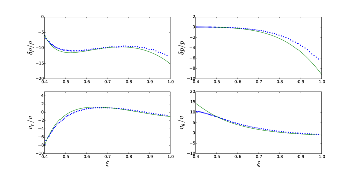
Figure 1: Comparison of the analytic (green solid line) and numeric profiles (blue dots) of the perturbed hydrodynamic variables: density (top left), pressure (top right), radial velocity (bottom left) and angular velocity (bottom right). The horizontal axis is the dimensionless radius (radius divided by the shock radius). The explosion parameters are $\gamma=\frac{5}{3}$, $\omega=0$, $q=0$, $l=1$, $\varepsilon=0.1$. In order to extract the information from the two dimensional simulations, we fit each ring to an expression of the form $A_{0}+A_{1}\cos\theta$ and plotted the ratio $\frac{A_{1}}{A_{0}}$ versus radius (except for the tangential velocity where we used $\sin\theta$ instead of $\cos\theta$, and normalized by the coefficient $A_{0}$ of the radial velocity). The inconsistency near the shock front stems from the fact that some of the ring is in the upstream.

3 Analytical Results for Special Cases

Though for a general choice of the parameters $\omega$, $q$, $l$ and $\gamma$ a numerical method must be employed to determine $d$, in some special cases it is possible to obtain an explicit analytic expression for $d$. In this section we will present few such cases which we were able to find.

3.1 Shifted Explosion

We consider a spherically symmetric explosion in a coordinate system where the origin is offset by $\varepsilon r_{0}\hat{z}$ to the hot spot. In such a coordinate system the ambient density profile, to first order in $\varepsilon$

$$\rho_{i}\left(r\right)\approx kr^{-\omega}\left(1+\omega\varepsilon\frac{r_{0}}{r}\cos\theta\right)$$ (18)

where $\cos\theta=\hat{r}\cdot\hat{z}$. The radius of the shock front, to first order in $\varepsilon$, is given accordingly by

$$R+\delta R=R\left(1+\varepsilon\cos\theta\right)$$ (19)

so

$$d\left(l=1,q=-1\right)=\omega$$ (20)

The hydrodynamic variables can be obtained from the unperturbed solutions in a similar manner

$$\delta P\left(\xi\right)=-P^{\prime}\left(\xi\right)$$ (21)

$$\delta G\left(\xi\right)=-G^{\prime}\left(\xi\right)$$ (22)

$$\delta U_{r}\left(\xi\right)=-\frac{U\left(\xi\right)}{\xi}-U^{\prime}\left(\xi\right)$$ (23)

$$\delta U_{t}\left(\xi\right)=-\frac{U\left(\xi\right)}{\xi}$$ (24)

It is easy to verify that these expressions satisfy the differential equations 8-11. This result supports the idea that at the center $\delta P=0$. The reason for that is that in the case of a filled type I explosion, the pressure plateaus as the radius approaches zero, so $\underset{\xi\rightarrow 0}{\lim}P^{\prime}\left(\xi\right)=0$ and hence $\delta P\left(0\right)=0$.

3.2 Thin Shell Model

In the limit $\gamma\rightarrow 1$ it is possible to use the thin shell approximation to find an analytic relation for $d$. Following [8], we define

$$\delta=\frac{\sigma-\sigma_{0}}{\sigma_{0}}$$ (25)

$$\Delta R=R-R_{0}$$ (26)

where

$$\sigma_{0}=\frac{1}{R^{2}}\int_{0}^{R}\rho r^{2}dr$$ (27)

$$\sigma=\frac{1}{\left(R+\delta R\right)^{2}}\int_{0}^{R+\delta R}\left(\rho+\delta\rho\right)r^{2}dr$$ (28)

are the unperturbed and perturbed surface density. The perturbation equations are

$$\frac{\partial\delta}{\partial t}=-\frac{2}{R_{0}}\frac{\partial\Delta R}{\partial t}+2\frac{\dot{R}_{0}}{R_{0}^{2}}\Delta R+\frac{\Delta\rho}{\sigma_{0}}\dot{R}_{0}-\omega\frac{\rho_{0}}{\sigma_{0}}\frac{\Delta R}{R_{0}}\dot{R}_{0}+\frac{\rho_{0}}{\sigma_{0}}\frac{\partial\Delta R}{\partial t}-\nabla_{T}\mathbf{v}_{T}-\delta\frac{\rho_{0}}{\sigma_{0}}\dot{R}_{0}$$ (29)

$$\frac{\partial^{2}\Delta R}{\partial t^{2}}=-\delta\dot{R}_{0}-2\frac{\rho_{0}\dot{R}_{0}}{\sigma_{0}}\frac{\partial\Delta R}{\partial t}-\frac{\Delta\rho\dot{R}_{0}^{2}}{\sigma_{0}}+\omega\frac{\rho_{0}}{\sigma_{0}}\frac{\Delta R}{R_{0}}\dot{R}_{0}^{2}$$ (30)

$$\frac{\partial\mathbf{v}_{T}}{\partial t}=-\frac{\rho_{0}\dot{R}_{0}}{\sigma_{0}}\mathbf{v}_{T}-\frac{\dot{R}_{0}}{R_{0}}\mathbf{v}_{T}-\frac{1}{R_{0}}\frac{P_{i}}{\sigma_{0}}\nabla_{T}\Delta R$$ (31)

where $\Delta\rho=\rho-\rho_{0}$. Assuming $\Delta\rho,\Delta R,\delta\propto Y_{lm}\left(\theta,\phi\right)R_{0}^{q}$ and $\mathbf{v}_{T}\propto\nabla_{T}Y_{lm}\left(\theta,\phi\right)R_{0}^{q}$ we can solve for the coefficients and find the parameter $d$ using the ratio $\Delta\rho/\Delta R$

$$d\left(\gamma=1\right)=(s+1)\left(\omega^{2}-8\omega+15\right)(s(\omega-5)+\omega-3)/$$ (32)

$$\left[4l\left(l+1\right)(\omega-3)^{2}+(s+1)(\omega-5)\left(s^{3}(\omega-5)^{3}+\right.\right.$$

$$\left.\left.s^{2}(5\omega-17)(\omega-5)^{2}+s\left(8\omega^{3}-90\omega^{2}+328\omega-390\right)+4(\omega-3)^{2}(\omega-2)\right)\right]$$

where $s=q\alpha$ and $\alpha=\frac{2}{5-\omega}$. This relation reproduces equation 20 for $l=1$ and $q=-1$.

3.3 Primakoff Solution

In the case of the Primakoff explosion, the perturbation equations can be solved analytically. With the substitution

$$\mathbf{Y}=\left(\frac{\delta G}{G},\frac{\delta P}{P},\frac{\delta U_{r}}{U},\frac{\delta U_{T}}{U}\right)^{T}$$ (33)

the system of ODEs can be reduced to the form

$$\frac{d\mathbf{Y}}{d\ln\xi}=\mathbf{M}\cdot\mathbf{Y}$$ (34)

$$\mathbf{M}=\left(\begin{array}[]{cccc}\frac{q(\gamma+1)^{2}+6(\gamma-1)}{\gamma^{2}-1}&-\frac{2(\gamma q+q+3\gamma-3)}{\gamma^{2}-1}&-\frac{2(\gamma q+q-\gamma+7)}{\gamma^{2}-1}&\frac{2l(l+1)}{\gamma+1}\\ \frac{6\gamma}{\gamma+1}&-\frac{\gamma q+q+6\gamma}{\gamma+1}&-\frac{2\left(q\gamma^{2}+(q+5)\gamma-3\right)}{\gamma^{2}-1}&\frac{2l(l+1)\gamma}{\gamma+1}\\ \frac{3(\gamma-1)}{\gamma+1}&-\frac{\gamma q+q+3\gamma-3}{\gamma+1}&-\frac{\gamma q+q+3\gamma+11}{\gamma+1}&\frac{2l(l+1)\gamma}{\gamma+1}\\ 0&1&0&\frac{\gamma q+q-3\gamma+5}{\gamma-1}\end{array}\right)$$ (35)

The general solution is

$$\mathbf{Y}\left(\xi\right)=\exp\left(\mathbf{M}\ln\xi\right)\mathbf{Y}\left(1\right)$$ (36)

Every term in $\mathbf{Y}\left(\xi\right)$ is the sum of 4 power laws in $\xi$, and the powers are eigenvalues. The value at the shock front is determined by the Rankine Hugoniot conditions (equations 12,13,14,15) and the inner boundary conditions that the pressure perturbation vanishes. Usually, out of the 4 eigenvector modes, one would diverge at the center (we denote the well behaved modes by $\mathbf{Y}_{1}$, $\mathbf{Y}_{2}$ and $\mathbf{Y}_{3}$, and the diverging mode by $\mathbf{Y}_{4}$). To prevent the divergence, we require that the solution will be a linear superposition of only the well behaved modes

$$\mathbf{Y}\left(1\right)=\sum_{i=1}^{3}a_{i}\mathbf{Y}_{i}$$ (37)

This gives us 4 linear equations with 4 variables ($a_{1}$,$a_{2}$, $a_{3}$ and $d$), from which we can extract the value of the paramter $d$. Unfortunately, the expression for the parameter $d$ is too long to be written here. We evaluate $d$ numerically as a function of both $q$ and $l$ for $\gamma=\frac{5}{3}$ and show the results in figure 2. If we interpret $q$ as the radial wave number, and $l$ as the angular wave number, then from figure 2 it seems that the magnitude of $d$ increases linearly with $q$ and $l$. Using the appropriate approximations for large $l$ reveals that in that limit $\underset{l\rightarrow\infty}{\lim}\frac{d}{l}=-\frac{\sqrt{2\gamma}}{\sqrt{\gamma+1}}$. We note that in the case of the Primakoff explosion the speed of sound vanishes at the center, whereas in the general filled type I explosion the speed of sound diverges there, so in the Primakoff explosion there are no reflections from the center, while the general case has them. For that reason, the general explosion does not have this asymptotic behavior.

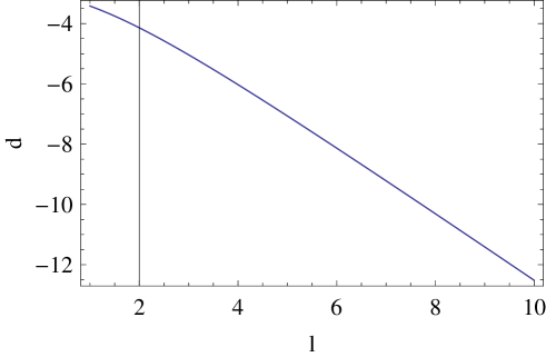
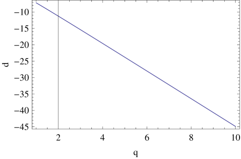
Figure 2: $d$ as a function of $l$ for $\gamma=\frac{5}{3}$ and $q=0$ (top) and $d$ as a function of $q$ for $\gamma=\frac{5}{3}$ (bottom), both for the Primakoff explosion

4 Extension to Arbitrary Angular Dependence

The formalism presented so far is limited to just one angular mode. However, due to linearity, any perturbation can be decomposed into spherical harmonics and each mode solved for individually. We demonstrate this using a problem similar to that used in the case of density perturbation to type II explosion [10]. The problem we are considering is an explosion that happens on the planar interface between two half spaces. Each half space has uniform density, but there is a slight difference between the densities of each of the half spaces. The ambient density profile can thus be described by the formula $\rho_{a}\left(r,\theta\right)=\rho_{0}\left(1+\sigma\Theta\left(\theta\right)\right)$, where $\Theta\left(x\right)$ is the Heaviside step function and $\sigma$ and $\rho_{0}$ are constants. Such expression can be expanded in spherical harmonics

$$\Theta\left(\theta\right)=\sum_{n=0}^{\infty}\frac{\pi\sqrt{4n+3}}{\Gamma\left(\frac{1}{2}-n\right)\Gamma\left(2+n\right)}Y_{2n+1,0}\left(\theta,0\right)$$ (38)

The shape of the perturbation to the shock front is given by

$$\frac{\delta R\left(\theta,t\right)}{R\left(t\right)}=\sigma\sum_{n=0}^{\infty}\frac{1}{d\left(2n+1\right)}\frac{\pi\sqrt{4n+3}}{\Gamma\left(\frac{1}{2}-n\right)\Gamma\left(2+n\right)}Y_{2n+1,0}\left(\theta,0\right)$$ (39)

In order to verify this result, we ran a numerical simulation for this scenario with $\sigma=0.1$ and compared it to the analytic result (equation 39) calculated up to order $n=100$. The results are plotted in figure 3, and there seems to be a good fit between the two methods, and they get closer as the resolution of the numerical simulation increases (the simulation we did had 1000 cells in the radial direction and 100 cells in the angular direction).

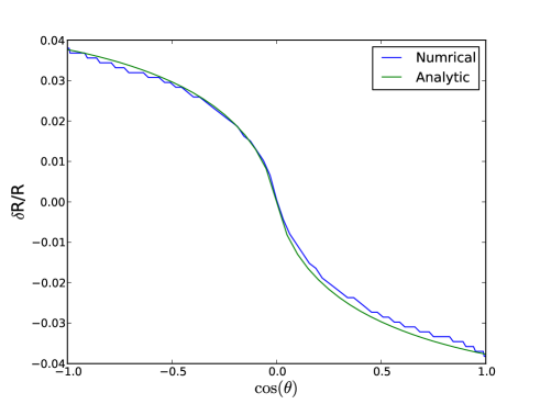
Figure 3: A comparison between the angular profiles of the analytic perturbation to the shock front (green) and the numerical simulation (blue) in case of an explosion between two uniform density half spaces with small density difference between them ($\sigma=\frac{\rho_{2}-\rho_{1}}{\rho_{1}}=0.1$).

5 Discussion

We have laid out a method for solving the strong explosion problem in density profiles that deviate from a pure radial power law dependence. The key lies in choosing radially log-periodic perturbations which do not introduce a new scale into the problem. This leads to self similar perturbation in the hydrodynamic quantities behind the shock, which can be found by solving a set of ordinary differential equations. The perturbations are fully self similar when the density perturbation is given in equation 2, but if $q$ is imaginary, then the solution is only discretely self similar because of the periodic nature of the perturbations.

The inner boundary condition in radial perturbation differs from that proposed here. We recall that in the case of radial perturbations to filled type I explosions the inner boundary condition is $\delta U_{r}\left(\xi=0\right)=0$, as given from the requirement that the total energy remains constant. This condition cannot be used for angular perturbation, because the total contribution of the perturbations to the energy is always zero for $l=0$. From the other end, the condition that the tangential velocity does not diverge cannot be applied to radial perturbations, as the tangential velocity is always zero.

The linearized perturbation treatment naturally ensures that the perturbations will be linear in $\varepsilon$ (and will contain no higher power of $\varepsilon$). This simplifies the solution of the problem but limits the validity of the method to small perturbations. The perturbation theory developed above fails when $\varepsilon$ becomes too large. The deviation from linear theory is of order $\varepsilon^{2}$.

References

- [1] I. B. Bernstein and D. L. Book. Stability of the Primakoff-Sedov blast wave and its generalizations. ApJ, 240:223–234, August 1980.
- [2] B. Gaffet. Stability of Self-Similar Flow - Correct Form of the Basic Equations and of the Shock Boundary Conditions. ApJ, 279:419, April 1984.
- [3] D. Kushnir, E. Waxman, and D. Shvarts. The Stability of Decelerating Shocks Revisited. ApJ, 634:407–418, November 2005.
- [4] L. D. Landau and E. M. Lifshitz. Fluid mechanics. 1959.
- [5] A. Mignone, G. Bodo, S. Massaglia, T. Matsakos, O. Tesileanu, C. Zanni, and A. Ferrari. PLUTO: A Numerical Code for Computational Astrophysics. apjs, 170:228–242, May 2007.
- [6] John Von Neumann, A. W. Taub, and A. H. Taub. The Collected Works of John Von Neumann: 6-Volume Set. Reader’s Digest Young Families, 1963.
- [7] Y. Oren and R. Sari. Discrete self-similarity in type-II strong explosions. Physics of Fluids, 21(5):056101–+, May 2009.
- [8] D. Ryu and E. T. Vishniac. The growth of linear perturbations of adiabatic shock waves. apj, 313:820–841, February 1987.
- [9] D. Ryu and E. T. Vishniac. The dynamic instability of adiabatic blast waves. apj, 368:411–425, February 1991.
- [10] R. Sari, N. Bode, A. Yalinewich, and A. MacFadyen. Slightly two- or three-dimensional self-similar solutions. Physics of Fluids, 24(8):087102, August 2012.
- [11] R. Sari, E. Waxman, and D. Shvarts. Shock Wave Stability in Steep Density Gradients. ApJS, 127:475–479, April 2000.
- [12] L. I. Sedov. Similarity and Dimensional Methods in Mechanics. 1959.
- [13] L. I. Sedov. Similarity methods and dimensional analysis in mechanics /8th revised edition/. Moscow Izdatel Nauka, 1977.
- [14] Geoffrey Taylor. The formation of a blast wave by a very intense explosion. i. theoretical discussion. Proceedings of the Royal Society of London. Series A. Mathematical and Physical Sciences, 201(1065):159–174, 1950.
- [15] E. Waxman and D. Shvarts. Second-type self-similar solutions to the strong explosion problem. Physics of Fluids, 5:1035–1046, April 1993.
- [16] Almog Yalinewich and Reem Sari. Discrete self similarity in filled type i strong explosions. Physics of Fluids (1994-present), 25(12):–, 2013.