Quantum Cellular Automaton Theory of Light

Abstract

We present a quantum theory of light based on quantum cellular automata (QCA). This approach allows us to have a thorough quantum theory of free electrodynamics encompassing an hypothetical discrete Planck scale. The theory is particularly relevant because it provides predictions at the macroscopic scale that can be experimentally tested. We show how, in the limit of small wave-vector $\mathbf{k}$, the free Maxwell’s equations emerge from two Weyl QCAs derived from informational principles in Ref. D’Ariano and Perinotti (2013). Within this framework the photon is introduced as a composite particle made of a pair of correlated massless Fermions, and the usual Bosonic statistics is recovered in the low photon density limit. We derive the main phenomenological features of the theory, consisting in dispersive propagation in vacuum, the occurrence of a small longitudinal polarization, and a saturation effect originated by the Fermionic nature of the photon. We then discuss whether these effects can be experimentally tested, and observe that only the dispersive effects are accessible with current technology, from observations of arrival times of pulses originated at cosmological distances.

I Introduction

The Quantum Cellular Automaton (QCA) is the quantum version of the popular cellular automaton of von Neumann von Neumann (1966). It describes the finite evolution of a discrete set of quantum systems, each one interacting with a finite number of neighbors via the unitary transformation of a single step evolution. The idea of a quantum version of a cellular automaton was already contained in the early work of Feynman Feynman (1982), and later has been object of investigation in the quantum-information community Schumacher and Werner (2004); Arrighi et al. (2011); Gross et al. (2012), with special enphasis on the so-called Quantum Walks (QW) which decribes the one particle sector of QCA’s with evolution linear in a quantum field Grossing and Zeilinger (1988); Succi and Benzi (1993); Meyer (1996); Bialynicki-Birula (1994); Ambainis et al. (2001).

The interest in QCAs is motivated by their potential applications in several fields, like the statistical mechanics of lattice systems and the quantum computation with microtraps Cirac and Zoller (2000) and with optical lattices Bloch (2004). Moreover, Quantum Walks have been used in the design of new quantum algorithms with a computational speed-up Childs et al. (2003); Farhi et al. (2007).

Recently, the idea that QCA could be used to describe a more fundamental discrete Plank scale dynamics from which the usual Quantum Field Theory emerges D’Ariano (2011); Bisio et al. (2012); D’Ariano and Perinotti (2013), is gathering increasing attention Farrelly and Short (2014); Arrighi et al. (2013). The proposal of modeling Planck scale physics with a classical automaton on a discrete background first appeared in the work of ’t Hooft ’t Hooft (1990), and Quantum Walks were considered for the simulation of Lorentz-covariant differential equations in Refs. Succi and Benzi (1993); Bialynicki-Birula (1994); Meyer (1996); Strauch (2006); Yepez (2006).

Up to now, most of the interest was focused on the emergence of the Dirac equation for a free Fermionic field. The choice of cosidering Fermions as the elementary physical systems is motivated by the idea that the amount of information that can be stored in a finite volume must be finite, as also suggested by black hole physics Bekenstein (1973); Hawking (1975). However, the question whether a Fermionic QCA could recover the dynamics of a Bosonic field was never addressed before. Here we will see how free electrodynamics emerges from two Weyl QCAs D’Ariano and Perinotti (2013) with Fermionic fields. The dynamical equations resulting in the limit of small wavevector $\mathbf{k}$ are the Maxwell’s equations. However, for high value of $\mathbf{k}$ the discreteness of the Planck scale manifests itself, producing deviations from Maxwell. Most notably, the QCA dynamics introduces a $\mathbf{k}$-dependent speed of light, a feature that was already considered in some approaches to quantum gravity, and that could be in principle experimentally detected in astrophysical observations Ellis et al. (1992); Lukierski et al. (1995); ’t Hooft (1996); Amelino-Camelia et al. (1998); Amelino-Camelia (2001); Amelino-Camelia and Piran (2001); Magueijo and Smolin (2002); Christiansen et al. (2006); Ellis and Mavromatos (2013).

In the present approach the photon turns out to be a composite particle made of a pair of correlated massless Fermions. This scenario closely resembles the neutrino theory of light of De Broglie De Broglie (1934); Jordan (1935); Kronig (1936); Perkins (1972, 2002) which suggested that the photon could be composed of a neutrino-antineutrino pair bound by some interaction. The failure of the neutrino theory of light was determined by the fact that a composite particle cannot obey the exact Bosonic commutation relations Pryce (1938). However, as it was shown in Ref. Perkins (2002), the non-Bosonic terms introduce negligible contribution at ordinary energy densities. In our case, as a consequence of the composite nature of the photon, we have that the number of photons that can occupy a single mode is bounded. However, as we will see, a saturation effect originated by the Fermionic nature of the photon is far beyond the current laser technology.

In Section II, after recalling some basic notions about the QCA,we review the Weyl automaton of Ref. D’Ariano and Perinotti (2013). In Section III we build a set of Fermionic bilinear operators, which in Sect. IV are proved to evolve according to the Maxwell equations. In Section V we will show that the polarization operators introduced in Sect. IV can be considered as Bosonic operators in a low energy density regime. As a spin-off of this analysis we found a result that completes the proof, given in Ref. Chudzicki et al. (2010), that the amount of entanglement quantifies whether pairs of Fermions can be considered as independent Bosons. Section VI presents the phenomenological consequences of the present QCA theory, the most relevant one being the the appearence of a $\mathbf{k}$-dependent speed of light. In the same section we discuss possible experimental tests of such $\mathbf{k}$-dependence in the astrophysical domain, and we compare our result with those from Quantum Gravity literature Ellis et al. (1992); Lukierski et al. (1995); ’t Hooft (1996); Amelino-Camelia et al. (1998); Amelino-Camelia (2001); Amelino-Camelia and Piran (2001); Magueijo and Smolin (2002); Christiansen et al. (2006); Ellis and Mavromatos (2013). We conclude with Section VII where we review the main results and discuss future developments.

II The Weyl automaton: a review

The basic ingredient of the Maxwell automaton is Weyl’s, whis has been derived in Ref. D’Ariano and Perinotti (2013) from first principles. Here, we will briefly review the construction for completeness.

A QCA represents the evolution of a numerable set $G$ of cells $g\in G$, each one containing an array of Fermionic local modes. The evolution occurs in discrete identical steps, and in each one every cell interacts with a the others. The Weyl automaton is derived from the following principles: unitarity, linearity, locality, homogeneity, transitivity, and isotropy. Unitarity means just that each step is a unitary evolution. Linearity means that the unitary evolution is linear in the field. Locality means that at each step every cell interacts with a finite number of others. We call cells interacting in one step neighbors. The neighboring notion also naturally defines a graph over the automaton, with $g$ as vertices and the neighboring couples as edges. Homogeneity means both that all steps are the same, all cells are identical systems, and the set of interactions with neigbours is the same for each cell, hence also the number of neigbours, and the dimension of the cell field array, which we will denote by $s>0$. We will denote by $A$ the matrix representing the linear unitary step. Transitivity means that every two cells are connected by a path of neighbours. Isotropy means that the neighboring relation is symmetric, and there exists a group of automorphisms for the graph for which the automaton itself is covariant. Homogeneity, transitivity, and isotropy together imply that $G$ is a group, and the graph is a Cayley graph $\Gamma(G,S_{+})$ where $G=\langle S_{+}|R\rangle$ is a presentation of $G$ with generator set $S_{+}$ and relator set $R$. The set of neighboring cells is then given by $S:=S_{+}\cup S_{-}$ where $S_{-}$ is the set of the inverse generators. Linearity, locality, and homogeneity imply that each step can be described in terms of transition matrices $A_{h}\in\rm{M}(\mathbb{C},s)$ for each $h\in S$, and then the step is described mathematically as follows

$$\psi_{g}(t+1)=\sum_{h\in S}A_{h}\psi_{hg}(t)$$ (1)

where $\psi_{g}(t)$ is the $s$-array of field operators at $g$ at step $t$. Therefore, upon denoting by $T_{g}$ $g\in G$ the unitary representation of $G$ on $\ell^{2}(G)$, $T_{g}|f\rangle:=|gf\rangle$, for $f\in G$, $A$ is a unitary operator on $\ell^{2}(G)\otimes\mathbb{C}^{s}$ of the form

$$A:=\sum_{h\in S}T_{h}\otimes A_{h}.$$ (2)

Covariance of the isotropy property means precisely that the group $L$ of automorphisms of the graph is a transitive permutation group of $S_{+}$, and there exists a (generally projective) unitary representation $U_{l}$ $l\in L$ of $L$ such that

$$A=\sum_{h\in S}T_{lh}\otimes U_{l}A_{h}U_{l}^{\dagger},\qquad\forall l\in L.$$ (3)

In Ref. D’Ariano and Perinotti (2013) attention was restricted to group $G$ quasi-isometrically embeddable in an Euclidean space, which is then virtually Abelian de Cornulier et al. (2007), namely it has an Abelian subgroup $G^{\prime}\subset G$ of finite index, namely with a finite number of cosets. Then it can be shown the automaton is equivalent to another one with group $G^{\prime}$ and dimension $s^{\prime}$ multiple of $s$. We further assume that the representation of the isotropy group $L$ induced by the embedding is orthogonal, which implies that the graph neighborhood is embedded in a sphere. We call such a property orthogonal isotropy.

For $s=1$ the automaton is trivial, namely $A=I$. For $s=2$ and for Euclidean space $\mathbb{R}^{3}$ one has $G=\mathbb{Z}^{3}$, and the Cayley graphs satisfying orthogonal isotropy are the Bravais lattices. The only lattice that has a nontrivial set of transition matrices giving a unitary automaton is the BCC lattice. We will label the group element as vectors $\mathbf{x}\in\mathbb{Z}^{3}$, and use the customary additive notation for the group composition, whereas the unitary representation of $\mathbb{Z}^{3}$ is expressed as follows

$$T_{\mathbf{z}}|\mathbf{x}\rangle=|\mathbf{z}+\mathbf{x}\rangle.$$ (4)

Being the group Abelian, we can Fourier transform, and the operator $A$ can be easily block-diagonalized in the $\mathbf{k}$ representation as follows

$$A=\int_{B}\operatorname{d}^{3}\!\mathbf{k}\,|{\mathbf{k}}\rangle\langle{\mathbf{k}}|\otimes A_{\mathbf{k}}$$ (5)

with $A_{\mathbf{k}}:=\sum_{\mathbf{h}\in S}\mathbf{k}\,e^{-i\mathbf{k}\cdot\mathbf{h}}A_{\mathbf{h}}$ unitary for every $\mathbf{k}\in B$, and the vectors $|{\mathbf{k}}\rangle$ given by

$$|\mathbf{k}\rangle:=\frac{1}{\sqrt{2\pi}^{3}}\sum_{\mathbf{x}\in G}e^{i\mathbf{k}\cdot\mathbf{x}}|\mathbf{x}\rangle,$$ (6)

is a Dirac-notation for the direct integral over $\mathbf{k}$, and the domain $B$ is the first Brillouin zone of the BCC. There are only two QCAs, with unitary matrices

$$A^{\pm}_{\mathbf{k}}:=d^{\pm}_{\mathbf{k}}I+\tilde{\mathbf{n}}^{\pm}_{\mathbf{k}}\cdot\boldsymbol{\sigma}=\exp[-i\mathbf{n}^{\pm}_{\mathbf{k}}\cdot\boldsymbol{\sigma}],$$ (7)

where

$$\tilde{\mathbf{n}}^{\pm}_{\mathbf{k}}:=\begin{pmatrix}s_{x}c_{y}c_{z}\mp c_{x}s_{y}s_{z}\\ \mp c_{x}s_{y}c_{z}-s_{x}c_{y}s_{z}\\ c_{x}c_{y}s_{z}\mp s_{x}s_{y}c_{z}\end{pmatrix}\!\!,\,{\mathbf{n}}^{\pm}_{\mathbf{k}}:=\frac{\lambda^{\pm}_{\mathbf{k}}\tilde{\mathbf{n}}^{\pm}_{\mathbf{k}}}{\sin\lambda^{\pm}_{\mathbf{k}}},$$

$$\operatorname{d}^{\pm}_{\mathbf{k}}:=(c_{x}c_{y}c_{z}\pm s_{x}s_{y}s_{z}),\;\lambda^{\pm}_{\mathbf{k}}:=\arccos(d^{\pm}_{\mathbf{k}}),$$

and

$$c_{\alpha}:=\cos({k}_{\alpha}/\sqrt{3}),\;s_{\alpha}:=\sin({k}_{\alpha}/\sqrt{3}),\;\alpha=x,y,z.$$

The matrices $A_{\mathbf{k}}^{\pm}$ in Eq. (7) describe the evolution of a two-component Fermionic field,

$${\psi}({\mathbf{k}},t+1)=A_{\mathbf{k}}^{\pm}{\psi}({\mathbf{k}},t),\quad{\psi}({\mathbf{k}},t):=\begin{pmatrix}{\psi}_{R}({\mathbf{k}},t)\\ {\psi}_{L}({\mathbf{k}},t)\end{pmatrix}.$$ (8)

The adimensional framework of the automaton corresponds to measure everything in Planck units. In such a case the limit $|{\mathbf{k}}|\ll 1$ corresponds to the relativistic limit, where on has

$$\mathbf{n}^{\pm}({\mathbf{k}})\sim\tfrac{{\mathbf{k}}}{\sqrt{3}},\quad A^{\pm}_{\mathbf{k}}\sim\exp[-i\tfrac{{\mathbf{k}}}{\sqrt{3}}\cdot\boldsymbol{\sigma}],$$ (9)

corresponding to the Weyl’s evolution, with $\tfrac{{\mathbf{k}}}{\sqrt{3}}$ playing the role of momentum.

III The Maxwell automaton

In order to build the Maxwell dynamics, we need to consider two different Weyl QCAs the first one acting on a Fermionic field $\psi(\mathbf{k})$ by matrix $A_{\mathbf{k}}$ as in Eq. (8), and the second one acting on the field $\varphi(\mathbf{k})$ by the complex conjugate matrix $A_{\mathbf{k}}^{*}=\sigma_{y}A_{\mathbf{k}}\sigma_{y}$, i.e.

$${\varphi}(\mathbf{k},t+1)=A_{\mathbf{k}}^{*}{\varphi}(\mathbf{k},t),\quad{\varphi}(\mathbf{k},t)=\begin{pmatrix}{\varphi}_{R}(\mathbf{k},t)\\ {\varphi}_{L}(\mathbf{k},t)\end{pmatrix}.$$ (10)

The matrix $A_{\mathbf{k}}$ can be either one of the Weyl matrices $A^{\pm}_{\mathbf{k}}$, and the whole derivation is independent of the choice.

The Fermionic fields ${\varphi}$ and ${\psi}$ are independent and obey the following anti-commutation relations

$$[\psi_{i}(\mathbf{k}),\psi_{j}(\mathbf{k}^{\prime})]_{+}=[\varphi_{i}(\mathbf{k}),\varphi_{j}(\mathbf{k}^{\prime})]_{+}=$$

$$[\varphi_{i}(\mathbf{k}),\psi_{j}(\mathbf{k}^{\prime})]_{+}=[\varphi_{i}(\mathbf{k}),\psi^{\dagger}_{j}(\mathbf{k}^{\prime})]_{+}=0$$

$$[\psi_{i}(\mathbf{k}),\psi^{\dagger}_{j}(\mathbf{k}^{\prime})]_{+}=[\varphi_{i}(\mathbf{k}),\varphi^{\dagger}_{j}(\mathbf{k}^{\prime})]_{+}=\delta_{B}(\mathbf{k}-\mathbf{k}^{\prime})\delta_{i,j}$$

$$i,j=R,L\qquad\mathbf{k},\mathbf{k}^{\prime}\in B,$$ (11)

where $\delta_{B}(\mathbf{k})$ is the 3d Dirac’s comb delta-distribution (which repeats periodically with $\mathbb{R}^{3}$ tasselated into Brillouin zones).

Given now two arbitrary fields ${\eta}(\mathbf{k})$ and ${\theta}(\mathbf{k})$ we define the following bilinear function

$$\!\!G_{f}^{\mu}(\eta,\theta,\mathbf{k}):=\!\!\int\!\!\frac{\operatorname{d}\mathbf{q}}{(2\pi)^{3}}f_{\mathbf{k}}(\mathbf{q}){{\eta}}^{T}\left(\tfrac{\mathbf{k}}{2}-\mathbf{q}\right)\sigma^{\mu}{\theta}\left(\tfrac{\mathbf{k}}{2}+\mathbf{q}\right)$$ (12)

where $\sigma^{0}:=I$, $\sigma^{1}:=\sigma^{x}$, $\sigma^{2}:=\sigma^{y}$, $\sigma^{3}:=\sigma^{z}$ and $\int\frac{\operatorname{d}\mathbf{q}}{(2\pi)^{3}}|f_{\mathbf{k}}(\mathbf{q})|^{2}=1,\forall\mathbf{k}$. In the following we will also treat the vector part $\boldsymbol{\sigma}:=(\sigma^{1},\sigma^{2},\sigma^{3})$ of the four-vector $\sigma^{\mu}$ separately. This allows us to define the following operators

$$F^{\mu}(\mathbf{k}):=G_{f}^{\mu}(\varphi,\psi,\mathbf{k})$$ (13)

In the following sections we study the evolution of the bilinear functions $F^{\mu}(\mathbf{k})$ and their commutation relations and show that, in the relativistic limit and for small particle densities the quantum Maxwell equations are recovered for both choices of $A_{\mathbf{k}}=A^{\pm}_{\mathbf{k}}$.

IV The Maxwell dynamics

In the following we will use the short notations

$$[Z\eta](\mathbf{k}):=Z_{\mathbf{k}}\eta(\mathbf{k}),\quad[ZW]_{\mathbf{k}}:=Z_{\mathbf{k}}W_{\mathbf{k}},$$ (14)

for $\eta$ a field and $Z$ and $W$ matrices. If the fields $\psi$ and $\varphi$ evolve according to Eqs. (8) and (10), then the evolution of the bilinear functions $F^{\mu}(\mathbf{k})$ introduced in Eq. (13) obeys the following equation

$$F^{\mu}(\mathbf{k},t)=G_{f}^{\mu}([{A^{*}}^{t}\varphi],[A^{t}\psi],\mathbf{k}),$$ (15)

where we used the notation in (14). Now, let us define

$$\tilde{F}^{\mu}(\mathbf{k},t):=G_{f}^{\mu}([{U^{\mathbf{k},t}}^{*}\varphi],[U^{\mathbf{k},t}\psi],\mathbf{k}),$$

$$U^{\mathbf{k},t}_{\mathbf{q}}:=A^{-t}_{\tfrac{\mathbf{k}}{2}}A^{t}_{\mathbf{q}},$$ (16)

where we remind that $[{U^{\mathbf{k},t}}^{*}\varphi](\mathbf{q}):={U_{\mathbf{q}}^{\mathbf{k},t}}^{*}\varphi(\mathbf{q})$. Clearly, one has $[A^{t}\eta]=[A_{\frac{\mathbf{k}}{2}}^{t}U^{\mathbf{k},t}\eta]$. We now need the identity

$$\exp(-\tfrac{i}{2}\mathbf{v}\cdot\boldsymbol{\sigma})\boldsymbol{\sigma}\exp(\tfrac{i}{2}\mathbf{v}\cdot\boldsymbol{\sigma})=\operatorname{Exp}(-i\mathbf{v}\cdot\mathbf{J})\boldsymbol{\sigma},$$

$$\exp(-\tfrac{i}{2}\mathbf{v}\cdot\boldsymbol{\sigma})\sigma^{0}\exp(\tfrac{i}{2}\mathbf{v}\cdot\boldsymbol{\sigma})=\sigma^{0},$$ (17)

where the matrix $\operatorname{Exp}(-i\mathbf{v}\cdot\mathbf{J})$ acts on $\boldsymbol{\sigma}$ regarded as a vector, and $\mathbf{J}=(J_{x},J_{y},J_{z})$ is the vector of angular momentum operators. We can then recast Eq. (15) in terms of the following functions

$$\mathbf{F}(\mathbf{k},t) :=(F^{1}(\mathbf{k},t),F^{2}(\mathbf{k},t),F^{3}(\mathbf{k},t))^{T},$$ (18)

and $\tilde{\mathbf{F}}(\mathbf{k},t)$ similarly defined, obtaining

$$F^{0}(\mathbf{k},t)=\tilde{F}^{0}(\mathbf{k},t),$$

$$\mathbf{F}(\mathbf{k},t)=\operatorname{Exp}\left(-2i{\mathbf{n}}_{\tfrac{\mathbf{k}}{2}}\cdot\mathbf{J}t\right)\tilde{\mathbf{F}}(\mathbf{k},t).$$ (19)

If we assume that

$$\int_{|\mathbf{q}|\geq\bar{q}(\mathbf{k})}\frac{\operatorname{d}\mathbf{q}}{(2\pi)^{3}}|f_{\mathbf{k}}(\mathbf{q})|^{2}\ll 1\quad\mbox{for}\ \bar{q}(\mathbf{k})\ll|\mathbf{k}|,$$ (20)

by taking the Taylor expansion of ${\mathbf{n}}_{\tfrac{\mathbf{k}}{2}+\mathbf{q}}$ with respect to $\mathbf{q}$ we can make the approximation

$${U}^{\mathbf{k},t}_{\tfrac{\mathbf{k}}{2}\pm\mathbf{q}} \simeq\exp\left(i{\mathbf{n}}_{\tfrac{\mathbf{k}}{2}}\cdot\boldsymbol{\sigma}t\right)\exp\left[-i\left({\mathbf{n}}_{\tfrac{\mathbf{k}}{2}}\pm\mathbf{l}_{\mathbf{k},\mathbf{q}}\right)\cdot\boldsymbol{\sigma}t\right]$$

$$\simeq\exp\left(\pm ic_{\mathbf{k},\mathbf{q}}\frac{{\mathbf{n}}_{\frac{\mathbf{k}}{2}}}{|{\mathbf{n}}_{\frac{\mathbf{k}}{2}}|}\cdot\boldsymbol{\sigma}t\right)+O\big{(}\tfrac{\bar{q}(\mathbf{k})}{|\mathbf{n}_{\frac{\mathbf{k}}{2}}|}\big{)},$$ (21)

where $\mathbf{l}_{\mathbf{k},\mathbf{q}}:=J_{{\mathbf{n}}}\left(\frac{\mathbf{k}}{2}\right)\mathbf{q}$ and $J_{{\mathbf{n}}}\left(\frac{\mathbf{k}}{2}\right)$ denotes the Jacobian matrix of the function $\mathbf{n}_{\mathbf{k}}$ evaluated at $\frac{\mathbf{k}}{2}$ and $c_{\mathbf{k},\mathbf{q}}:=\frac{{\mathbf{n}}_{\frac{\mathbf{k}}{2}}}{|{\mathbf{n}}_{\frac{\mathbf{k}}{2}}|}\cdot\mathbf{l}_{\mathbf{k},\mathbf{q}}$ (the proof of Eq. 21 is given in Appendix A). By introducing the transverse field operators

$$\begin{split}\tilde{\mathbf{F}}_{T}(\mathbf{k},t):=\tilde{\mathbf{F}}(\mathbf{k},t)-\left(\frac{\mathbf{n}_{\frac{\mathbf{k}}{2}}}{|\mathbf{n}_{\frac{\mathbf{k}}{2}}|}\cdot\tilde{\mathbf{F}}(\mathbf{k},t)\right)\frac{\mathbf{n}_{\frac{\mathbf{k}}{2}}}{|\mathbf{n}_{\frac{\mathbf{k}}{2}}|}\\ \mathbf{F}_{T}(\mathbf{k},t):=\mathbf{F}(\mathbf{k},t)-\left(\frac{\mathbf{n}_{\frac{\mathbf{k}}{2}}}{|\mathbf{n}_{\frac{\mathbf{k}}{2}}|}\cdot{\mathbf{F}}(\mathbf{k},t)\right)\frac{\mathbf{n}_{\frac{\mathbf{k}}{2}}}{|\mathbf{n}_{\frac{\mathbf{k}}{2}}|}.\end{split}$$ (22)

and using Eq. (21) into Eq. (18) we get (see Appendix B)

$$\begin{split}\tilde{\mathbf{F}}_{T}(\mathbf{k},t)={\mathbf{F}}_{T}(\mathbf{k})+O\big{(}\tfrac{\bar{q}(\mathbf{k})}{|\mathbf{n}_{\frac{\mathbf{k}}{2}}|}\big{)}.\end{split}$$ (23)

Finally, combining Eq. (23) with Eq. (IV) we obtain a closed expression for the time evolution of the operator ${\mathbf{F}_{T}}(\mathbf{k})$,

$$\begin{split}\mathbf{F}_{T}(\mathbf{k},t)=\exp\left[\left(2\mathbf{n}_{\tfrac{\mathbf{k}}{2}}\cdot\mathbf{J}\right)t\right]{\mathbf{F}_{T}}(\mathbf{k})+\Lambda(\mathbf{k},t),\end{split}$$ (24)

where $\|\Lambda(\mathbf{k},t)\|=O\big{(}\tfrac{\bar{q}(\mathbf{k})}{|\mathbf{n}_{\frac{\mathbf{k}}{2}}|}\big{)}$. Taking the time derivative in Eq. (24) and reminding the definition (22) we obtain

$$\begin{split}&\partial_{t}\mathbf{F}_{T}(\mathbf{k},t)=2\mathbf{n}_{\frac{\mathbf{k}}{2}}\times\mathbf{F}_{T}(\mathbf{k},t)+\partial_{t}\Lambda(\mathbf{k},t)\\ &2\mathbf{n}_{\frac{\mathbf{k}}{2}}\cdot\mathbf{F}_{T}(\mathbf{k},t)=0,\end{split}$$ (25)

where $\|\partial_{t}\Lambda(\mathbf{k},t)\|=O\big{(}\tfrac{\bar{q}(\mathbf{k})}{|\mathbf{n}_{\frac{\mathbf{k}}{2}}|}\big{)}$ (see Appendix B).

Let now $\mathbf{E}$ and $\mathbf{B}$ be two Hermitian operators defined by the relation

$$\mathbf{E}:=|{\mathbf{n}}_{\tfrac{\mathbf{k}}{2}}|(\mathbf{F}_{T}+\mathbf{F}_{T}^{\dagger}),\quad\mathbf{B}:=i|{\mathbf{n}}_{\tfrac{\mathbf{k}}{2}}|(\mathbf{F}_{T}^{\dagger}-\mathbf{F}_{T}),$$

$$2|{\mathbf{n}}_{\tfrac{\mathbf{k}}{2}}|\mathbf{F}_{T}=\mathbf{E}+i\mathbf{B}.$$ (26)

We now show that in the limit of small wavevectors $\mathbf{k}$ and by interpreting $\mathbf{E}$ and $\mathbf{B}$ as the electric and magnetic field the usual vacuum Maxwell’s equations can be recovered. For $|\mathbf{k}|\ll 1$ one has $2\mathbf{n}_{\frac{\mathbf{k}}{2}}\simeq\mathbf{k}/\sqrt{3}$, and Eq. (LABEL:eq:maxwell2) becomes

$$\begin{split}&\partial_{t}\mathbf{F}_{T}(\mathbf{k},t)=\frac{\mathbf{k}}{\sqrt{3}}\times\mathbf{F}_{T}(\mathbf{k},t)\\ &\mathbf{k}\cdot\mathbf{F}_{T}(\mathbf{k},t)=0\end{split}\;.$$ (27)

As in Ref. D’Ariano and Perinotti (2013), we recover physical dimensions from the previous adimensional equations using Planck units, taking $c:=l_{P}/t_{P}$, time measured in Planck times $t\to t*t_{P}$, and lengths measured in Planck lenghts as $x\to x*\sqrt{3}l_{P}$, the $\sqrt{3}l_{P}$ corresponding to the distance between neighboring cells. Then Eq. (LABEL:eq:maxwell3) becomes

$$\begin{split}&\partial_{t}\mathbf{F}_{T}(\mathbf{x},t)=-ic\nabla\times\mathbf{F}_{T}(\mathbf{x},t)\\ &\nabla\cdot\mathbf{F}_{T}(\mathbf{x},t)=0\end{split}$$ (28)

which in terms of $\mathbf{E}$ and $\mathbf{B}$ become the vacuum Maxwell’s equations

$$\begin{array}[]{lcl}\nabla\cdot\mathbf{E}=0&&\nabla\cdot\mathbf{B}=0\\ \partial_{t}\mathbf{E}=c\nabla\times\mathbf{B}&&\partial_{t}\mathbf{B}=-c\nabla\times\mathbf{E}\;\;.\end{array}$$ (31)

Introducing the polarization vectors $\mathbf{u}_{\mathbf{k}}^{1}$ and $\mathbf{u}_{\mathbf{k}}^{2}$ satisfying

$$\mathbf{u}^{i}_{\mathbf{k}}\cdot\mathbf{n}_{\mathbf{k}}=\mathbf{u}^{1}_{\mathbf{k}}\cdot\mathbf{u}^{2}_{\mathbf{k}}=0,\ |\mathbf{u}^{i}_{\mathbf{k}}|=1,\ (\mathbf{u}^{1}_{\mathbf{k}}\times\mathbf{u}^{2}_{\mathbf{k}})\cdot\mathbf{n}_{\mathbf{k}}>0,$$ (32)

we can now interpret the following operators

$$\gamma^{i}(\mathbf{k}) :=\mathbf{u}^{i}_{\mathbf{k}}\cdot\mathbf{F}(\mathbf{k},0),\quad i=1,2,$$ (33)

as the two polarization operators of the field. In the light of this analysis, one can conclude that the automaton discrete evolution leads to modified Maxwell’s equations in the form of Eqs. (LABEL:eq:maxwell2), with the electromagnetic field rotating around $\mathbf{n}_{\tfrac{\mathbf{k}}{2}}$ instead of $\mathbf{k}$. Moreover, since in this framework the photon is a composite particle, the internal dynamics of the consitutent Fermions is responsible for an additional term $O\big{(}\tfrac{\bar{q}(\mathbf{k})}{|\mathbf{n}_{\frac{\mathbf{k}}{2}}|}\big{)}$. As a consequence of this distorsion, one can immediately see that the electric and magnetic fields are no longer exactly transverse to the wave vector but we have the appearence of a longitudinal component of the polarization (see Fig. 1). In Section VI we discuss the new phenomenology that emerges from Eqs. (LABEL:eq:maxwell2).

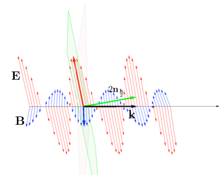
Figure 1: (colors online) A rectilinear polarized electromagnetic wave. We notice that the polarization plane (in green) is sligtly tilted with respect the plane orthogonal to $\mathbf{k}$ (in gray).

V Photons as composite Bosons

In the previous section we proved that the operators defined in Eq. (IV) dynamically evolve according to the free Maxwell’s equation. However, in order to interpret $\mathbf{E}(\mathbf{k})$ and $\mathbf{B}(\mathbf{k})$ as the electric and magnetic fields we need to show that they obey the correct commutation relation. The aim of this paragraph is to show that, in a regime of low energy density, the polarization operators defined in Eq. (33) actually behave as independent Bosonic modes.

In order to avoid the technicalities of the continuum we now suppose to confine the system in finite volume $\mathcal{V}$. The finiteness of the volume introduces a discretization of the momentum space and the operators $\psi(\mathbf{k})$, $\varphi(\mathbf{k})$, obey Eq. (11) where the periodic Dirac delta is replaced by the Kronecker delta. All the integrals over the Brillouin zone are then replaced by sums, and the polarization operators of Eq. (33) become

$$\gamma^{i}(\mathbf{k}):=\sum_{\mathbf{q}}f_{\mathbf{k}}(\mathbf{q}){\varphi}^{T}\left(\tfrac{\mathbf{k}}{2}-\mathbf{q}\right)(\mathbf{u}^{i}_{\tfrac{\mathbf{k}}{2}}\cdot\boldsymbol{\sigma}){\psi}\left(\tfrac{\mathbf{k}}{2}+\mathbf{q}\right).$$ (34)

These operators can be simply expressed in terms of the functions $\gamma_{\alpha,\beta}(\mathbf{k})$ defined as follows

$$\gamma_{\alpha,\beta}(\mathbf{k}):=\sum_{\mathbf{q}}{f}_{\mathbf{k}}(\mathbf{q})\varphi_{\alpha}\left(\tfrac{\mathbf{k}}{2}-\mathbf{q}\right)\psi_{\beta}\left(\tfrac{\mathbf{k}}{2}+\mathbf{q}\right),$$

$$\alpha,\beta=R,L.$$ (35)

Since the polarisation operators $\gamma^{i}(\mathbf{k})$ are linear combinations of $\gamma_{\alpha,\beta}(\mathbf{k})$, it is useful to compute the commutation relations of the latter. We have

$$[\gamma_{\alpha,\beta}(\mathbf{k}),\gamma_{\alpha^{\prime},\beta^{\prime}}(\mathbf{k}^{\prime})]_{-}=0,$$

$$[\gamma_{\alpha,\beta}(\mathbf{k}),\gamma^{\dagger}_{\alpha^{\prime},\beta^{\prime}}(\mathbf{k}^{\prime})]_{-}=\delta_{\alpha,\alpha^{\prime}}\delta_{\beta,\beta^{\prime}}\delta_{\mathbf{k},\mathbf{k}^{\prime}}-\Delta_{\alpha,\alpha^{\prime},\beta,\beta^{\prime},\mathbf{k},\mathbf{k}^{\prime}},$$

$$\Delta_{\alpha,\alpha^{\prime},\beta,\beta^{\prime},\mathbf{k},\mathbf{k}^{\prime}}:=\left(\delta_{\alpha,\alpha^{\prime}}H^{+}_{\psi,\beta^{\prime},\beta,\mathbf{k}^{\prime},\mathbf{k}}+\delta_{\beta,\beta^{\prime}}H^{-}_{\varphi,\alpha^{\prime},\alpha,\mathbf{k}^{\prime},\mathbf{k}}\right),$$

$$H^{\pm}_{\eta,\alpha^{\prime},\alpha,\mathbf{k}^{\prime},\mathbf{k}}:=\sum_{\mathbf{q}}{f}_{\mathbf{k}}(\mathbf{q}){f}_{\mathbf{k}^{\prime}}^{*}(\tfrac{\mathbf{k}^{\prime}-\mathbf{k}}{2}+\mathbf{q})$$

$$\qquad\times\eta_{\alpha^{\prime}}^{\dagger}\left(\tfrac{2\mathbf{k}^{\prime}-\mathbf{k}}{2}\pm\mathbf{q}\right)\eta_{\alpha}\left(\tfrac{\mathbf{k}}{2}\pm{\mathbf{q}}\right).$$ (36)

Then the operators $\gamma_{\alpha,\beta}$ fail to be Bosonic annihilation operators because of the apperance of the operator $\Delta_{\alpha,\alpha^{\prime},\beta,\beta^{\prime},\mathbf{k},\mathbf{k}^{\prime}}$ in the commutation relation (V). However, if we restrict to the subset $\mathcal{S}$ of states such that $\operatorname{Tr}[\rho H^{-}_{\varphi,\beta^{\prime},\beta,\mathbf{k}^{\prime},\mathbf{k}}]\simeq 0$ and $\operatorname{Tr}[\rho H^{+}_{\psi,\alpha^{\prime},\alpha,\mathbf{k}^{\prime},\mathbf{k}}]\simeq 0$ for all $\rho\in\mathcal{S}$, we could make the approximation $[\gamma_{\alpha,\beta}(\mathbf{k}),\gamma^{\dagger}_{\alpha^{\prime},\beta^{\prime}}(\mathbf{k}^{\prime})]_{-}\simeq\delta_{\alpha,\alpha^{\prime}}\delta_{\beta,\beta^{\prime}}\delta_{\mathbf{k},\mathbf{k}^{\prime}}$. If we consider the modulus of the expectation value of the operators $H^{\pm}_{\eta,\beta^{\prime},\beta,\mathbf{k}^{\prime},\mathbf{k}}$ we have

$$|\langle H^{\pm}_{\eta,\beta^{\prime},\beta,\mathbf{k}^{\prime},\mathbf{k}}\rangle|\leq\sum_{\mathbf{q}}\left|{f}_{\mathbf{k}}(\mathbf{q})\right|\left|{f}_{\mathbf{k}^{\prime}}^{*}(\tfrac{\mathbf{k}^{\prime}-\mathbf{k}}{2}+\mathbf{q})\right|$$

$$\quad\times\left|\left\langle\eta_{\beta^{\prime}}^{\dagger}\left(\tfrac{2\mathbf{k}^{\prime}-\mathbf{k}}{2}\pm\mathbf{q}\right)\eta_{\beta}\left(\tfrac{\mathbf{k}}{2}\pm\mathbf{q}\right)\right\rangle\right|\leq$$

$$\qquad\sqrt{\langle\Gamma^{\pm}_{\eta,\beta,\mathbf{k}}\rangle\langle\Gamma^{\pm}_{\eta,\beta^{\prime},\mathbf{k}^{\prime}}\rangle},$$ (37)

$$\Gamma^{\pm}_{\eta,\beta,\mathbf{k}}=\sum_{\mathbf{q}}\left|{f}_{\mathbf{k}}(\mathbf{q})\right|^{2}\eta^{\dagger}_{\beta}\left(\tfrac{\mathbf{k}}{2}\pm\mathbf{q}\right)\eta_{\beta}\left(\tfrac{\mathbf{k}}{2}\pm\mathbf{q}\right),$$ (38)

where we repeatedly applied the Schwartz inequality.

The operators $\Gamma^{-}_{\varphi,\beta,\mathbf{k}}$ and $\Gamma^{+}_{\psi,\alpha,\mathbf{k}}$ can be interpreted as number operators “shaped” by the probability distribution $|{f}_{\mathbf{k}}(\mathbf{q})|^{2}$. If we suppose $|{f}_{\mathbf{k}}(\mathbf{q})|^{2}$ to be a constant function over a region $\Omega_{\mathbf{k}}$ which contains $N_{\mathbf{k}}$ modes, i.e. $|{f}_{\mathbf{k}}(\mathbf{q})|^{2}=\tfrac{1}{N_{\mathbf{k}}}$ if $\mathbf{q}\in\Omega_{\mathbf{k}}$ and $|{f}_{\mathbf{k}}(\mathbf{q})|^{2}=0$ if $\mathbf{q}\not\in\Omega_{\mathbf{k}}$, we have

$$\left\langle\Gamma^{+}_{\psi,\alpha,\mathbf{k}}\right\rangle=\frac{1}{N_{\mathbf{k}}}\sum_{\mathbf{q}\in\Omega_{\mathbf{k}}}\left\langle\psi^{\dagger}_{\alpha}\left(\tfrac{\mathbf{k}}{2}+\mathbf{q}\right)\psi_{\alpha}\left(\tfrac{\mathbf{k}}{2}+\mathbf{q}\right)\right\rangle=\frac{M_{\psi,\alpha,\mathbf{k}}}{N_{\mathbf{k}}}$$

where we denoted with $M_{\psi,\alpha,\mathbf{k}}$ the number of $\psi_{\alpha}$ Fermions in the region $\Omega_{k}$ (clearly the same result applies to $\Gamma^{-}_{\varphi,\beta,\mathbf{k}}$). Then, if we consider states $\rho$ such that $M_{\xi,\chi,\mathbf{k}}/N_{\mathbf{k}}\leq\varepsilon$ for all $\xi_{\chi}$ and $\mathbf{k}$ and for $\varepsilon\ll 1$ we can safely assume $[\gamma_{\alpha,\beta}(\mathbf{k}),\gamma^{\dagger}_{\alpha^{\prime},\beta^{\prime}}(\mathbf{k}^{\prime})]_{-}=\delta_{\alpha,\alpha^{\prime}}\delta_{\beta,\beta^{\prime}}\delta_{\mathbf{k},\mathbf{k}^{\prime}}$ in Eq. (V) which after an easy calculation gives

$$[\gamma^{i}(\mathbf{k}),{\gamma^{j}}^{\dagger}(\mathbf{k}^{\prime})]_{-}=\delta_{i,j}\delta_{\mathbf{k},\mathbf{k}^{\prime}}\quad i=0,1,2,3.$$ (39)

In Eq. (39), besides the previously defined transverse polarizations $\gamma^{1}(\mathbf{k})$ and $\gamma^{2}(\mathbf{k})$, we considered also the “longitudinal” polarization operator $\gamma^{3}(\mathbf{k}):=\sum_{\mathbf{q}}f_{\mathbf{k}}(\mathbf{q}){\varphi}^{T}\left(\tfrac{\mathbf{k}}{2}-\mathbf{q}\right)(\mathbf{e}_{\tfrac{\mathbf{k}}{2}}\cdot\boldsymbol{\sigma}){\psi}\left(\tfrac{\mathbf{k}}{2}+\mathbf{q}\right)$, where $\mathbf{e}_{\mathbf{k}}:=\mathbf{n}_{\mathbf{k}}/|\mathbf{n}_{\mathbf{k}}|$, and the “timelike” polarization operator $\gamma^{0}(\mathbf{k}):=\sum_{\mathbf{q}}{f}_{\mathbf{k}}(\mathbf{q}){\varphi}^{T}\left(\tfrac{\mathbf{k}}{2}-\mathbf{q}\right)I{\psi}\left(\tfrac{\mathbf{k}}{2}+\mathbf{q}\right)$.

This result tells us that, as far as we restrict ourselves to states in $\mathcal{S}$ we are allowed to interpret the operators $\gamma^{i}(\mathbf{k})$ as $4$ independent Bosonic field modes and then to interpret $\mathbf{E}$ and $\mathbf{B}$ defined in Eq. (IV) as the electric and the magnetic field operators. This fact together with the evolution given by Eq. (LABEL:eq:maxwell3) proves that we realized a consistent model of quantum electrodynamics in which the photons are composite particles made by correlated Fermions whose evolution is described by a cellular automaton.

V.1 Composite Bosons and entanglement

The results that we had in this section are in agreement with the recent works Combescot and Tanguy (2001); Rombouts et al. (2002); Avancini et al. (2003); Combescot et al. (2003) which studied the conditions under which a pair of Fermionic fields can be considered as a Boson. In Refs. Law (2005); Chudzicki et al. (2010) it was shown that a sufficient condition is that the two Fermionic fields $\psi,\phi$ are sufficiently entangled. More precisely, for a composite Boson $c:=\sum_{i}f(i)\psi_{i}\phi_{i}$, $\sum_{i}|f(i)|^{2}=1$ one has

$$[c,c^{\dagger}]=1-(\Gamma_{\psi}+\Gamma_{\phi}),$$ (40)

where

$$\Gamma_{\psi}=\sum_{i}|f(i)|^{2}\psi^{\dagger}_{i}\psi_{i},\quad\Gamma_{\phi}=\sum_{i}|f(i)|^{2}\phi^{\dagger}_{i}\phi_{i},$$ (41)

and in Ref. Chudzicki et al. (2010) it was shown that the following bound holds

$$\forall N\geq 1,\quad NP\geq\langle{N}|\Gamma_{\psi}|{N}\rangle\geq P,$$ (42)

and the same holds for $\Gamma_{\phi}$, where $P=\sum_{i=1}^{N}|f(i)|^{4}$ is the purity of the reduced state of a single particle and $|{N}\rangle=\tfrac{1}{\sqrt{N!}}\chi_{N}(c^{\dagger})^{N}|{0}\rangle$ ($\chi_{N}$ is a normalization constant). From this result, the authors of Ref. Chudzicki et al. (2010) concluded that, as far as $P,NP\approx 0$, $c$ and $c^{\dagger}$ can be safely considered as a Bosonic annihilation/creation pair. Our criterion, which restricts the state $\rho$ to satisfy $\operatorname{Tr}[\rho\Gamma_{\psi}],\operatorname{Tr}[\rho\Gamma_{\phi}]\leq\varepsilon$ in this simplified scenario, gives the criterion in Refs. Law (2005); Chudzicki et al. (2010) for $\rho=|N\rangle\langle N|$. Moreover it is interesting to show that the technique applied in the derivation of Eq. (V) can be used to answer an open question raised in Ref. Chudzicki et al. (2010). The conjecture is that, given two different composite Bosons $c_{1}=\sum_{i}f_{1}(i)\psi_{i}\phi_{i}$ and $c_{2}=\sum_{i}f_{2}(i)\psi_{i}\phi_{i}$ such that $\sum_{i}f_{1}(i)f_{2}(i)^{*}=0$, the commutation relation $[c_{1},c_{2}^{\dagger}]$ should vanish as the two purities $P_{1}$ and $P_{2}$ ($P_{a}=\sum_{i=1}^{N}|f_{a}(i)|^{4}$) decrease. Since $[c_{1},c_{2}^{\dagger}]=-\sum_{i}f_{1}(i)f_{2}(i)^{*}(\psi_{i}^{\dagger}\psi_{i}+\phi_{i}^{\dagger}\phi_{i})$ we have

$$|\langle[c_{1},c_{2}^{\dagger}]\rangle|\leq\sum_{x}\sqrt{\langle\Gamma^{(1)}_{x}\rangle\langle\Gamma^{(2)}_{x}\rangle},$$ (43)

by the same reasoning that we followed in the derivation of Eq. (V). Combining this last inequality with the condition $\langle N|\Gamma^{(i)}_{x}|N\rangle\leq NP$ we have $|\langle N|[c_{1},c_{2}^{\dagger}]|N\rangle|\leq 2NP$ which proves the conjecture.

VI Phenomenological analysis

We now investigate the new phenomenology predicted from the modified Maxwell equations (LABEL:eq:maxwell2) and the modified commutation relations (V), with a particular focus on practically testable effects.

Let us first have a closer look at the dynamics described by Eq. (24). If $\mathbf{u}_{+}$ and $\mathbf{u}_{-}$ are the two eigenvectors of the matrix $\operatorname{Exp}[(2\mathbf{n}_{\frac{\mathbf{k}}{2}}\cdot\mathbf{J})t]$, corresponding to eigenvalues $e^{\mp i2|\mathbf{n}_{\frac{\mathbf{k}}{2}}|t}$, Eq. (24) can be written as

$$\mathbf{F}_{T}(\mathbf{k},t)=e^{-i2|\mathbf{n}_{\frac{\mathbf{k}}{2}}|t}\gamma_{+}(\mathbf{k})\mathbf{u}_{+}+e^{i2|\mathbf{n}_{\frac{\mathbf{k}}{2}}|t}\gamma_{-}(\mathbf{k})\mathbf{u}_{-}$$ (44)

where the corresponding polarization operators $\gamma_{\pm}(\mathbf{k})$ are defined according to Eq. (33). According to Eq. (44) the angular frequency of the electromagnetic waves is given by the modified dispersion relation

$$\omega(\mathbf{k})=2|\mathbf{n}_{\tfrac{\mathbf{k}}{2}}|.$$ (45)

The usual relation $\omega(\mathbf{k})=|\mathbf{k}|$ is recovered in the $|\mathbf{k}|\ll 1$ regime. The speed of light is the group velocity of the electromagnetic waves, i.e. the gradient of the dispersion relation. The major consequence of Eq. (45) is that the speed of light depends on the value of $\mathbf{k}$, as for Maxwell’s equations in a dispersive medium.

The phenomenon of a $\mathbf{k}$-dependent speed of light was already analyzed in the in the context of quantum gravity where many authors considered the hypothesis that the existence of an invariant length (the Planck scale) could manifest itself in terms of modified dispersion relations Ellis et al. (1992); Lukierski et al. (1995); ’t Hooft (1996); Amelino-Camelia (2001); Magueijo and Smolin (2002). In these models the $\mathbf{k}$-dependent speed of light $c(\mathbf{k})$, at the leading order in $k:=|\mathbf{k}|$, is expanded as $c(\mathbf{k})\approx 1\pm\xi k^{\alpha}$, where $\xi$ is a numerical factor of order $1$, while $\alpha$ is an integer. This is exactly what happens in our framework, where the intrinsic discreteness of the quantum cellular automata $A^{\pm}$ leads to the dispersion relation of Eq. (45) from which the following $\mathbf{k}$-dependent speed of light

$$c^{\mp}(\mathbf{k})\approx 1\pm 3\frac{k_{x}k_{y}k_{z}}{|\mathbf{k}|^{2}}\approx 1\pm\tfrac{1}{\sqrt{3}}k,$$ (46)

can be obtained by computing the modulus of the group velocity and power expanding in $\mathbf{k}$ with the assumption $k_{x}=k_{y}=k_{z}=\tfrac{1}{\sqrt{3}}k$, ($k=|\mathbf{k}|$). It is interesting to observe that depending on the automaton $A^{+}(\mathbf{k})$ of $A^{-}(\mathbf{k})$ in Eq. (7) we obtain corrections to the speed of light with opposite sign. Moreover the correction is not isotropic and can be superluminal, though uniformly bounded for all $\mathbf{k}$ as shown for the Weyl automaton in Ref. D’Ariano and Perinotti (2013).

Models leading to modified dispersion relations recently received attention because they allow one to derive falsifiable predictions of the Plank scale hypothesis. These can be experimentally tested in the astrophysical domain, where the tiny corrections to the usual relativistic dynamics can be magnified by the huge time of flight. For example, observations of the arrival times of pulses originated at cosmological distances, like in some $\gamma$-ray burstsAmelino-Camelia et al. (1998); Abdo et al. (2009); Vasileiou et al. (2013); Amelino-Camelia and Smolin (2009), are now approaching a sufficient sensitivity to detect corrections to the relativistic dispersion relation of the same order as in Eq. (46).

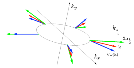
Figure 2: (colors online) The graphics shows the vector $2\mathbf{n}_{\tfrac{\mathbf{k}}{2}}$ (in green), which is orthogonal to the polarization plane, the wavevector $\mathbf{k}$ (in red) and the group velocity $\nabla\omega(\mathbf{k})$ (in blue) as function of $\mathbf{k}$ for the value $|\mathbf{k}|=0.8$ and different directions. Notice that the three vectors are not parallel and the angles between them depend on $\mathbf{k}$. Such anisotropic behavior can be traced back to the anisotropy of the dispersion relation of the Weyl automaton.

A second distinguishing feature of Eq. (LABEL:eq:maxwell2) is that the polarization plane is neither orthogonal to the wavevector, nor to the group velocity, which means that the electromagnetic waves are no longer exactly transverse (see Figs. 1 and 2). However the angle $\theta$ between the polarization plane and the plane orthogonal to $\mathbf{k}$ or $\nabla\omega(\mathbf{k})$ is of the order $\theta\approx 2k$, which gives $10^{-15}\mathrm{rad}$ for a $\gamma$-ray wavelength, a precision which is not reachable by the present technology. Since for a fixed $\mathbf{k}$ the polarization plane is constant, exploiting greater distances and longer times does not help in magnifying this deviation from the usual electromagnetic theory.

Finally, the third phenomenological consequence of our modelling is that, since the photon is described as a composite Boson, deviations from the usual Bosonic statistics are in order. As we proved in Section V, the choice of the function ${f}_{\mathbf{k}}(\mathbf{q})$ determines the regime where the composite photon can be approximately treated as a Boson. However, independently on the details of function ${f}_{\mathbf{k}}(\mathbf{q})$ one can easily see that a Fermionic saturation of the Boson is not visible, e.g. for the most powerful laser Dunne (2007) one has a approximately an Avogadro number of photons in $10^{-15}$cm³, whereas in the same volume on has around $10^{90}$ Fermionic modes.

Another test for the composite nature of photons is provided by the prediction of deviations from the Planck’s distribution in Blackbody radiation experiments. A similar analysis was carried out in Ref. Perkins (2002), where the author showed that the predicted deviation from Planck’s law is less than one part over $10^{-8}$, well beyond the sensitivity of present day experiments.

VII Conclusions

In this paper we derive a complete theoretical framework of the free quantum radiation field at the Planck scale, based on a quantum Weyl automaton derived from first principles in Ref. D’Ariano and Perinotti (2013). Differently from previous arguments based just on discreteness of geometry, the present approach provides fully quantum theoretical treatment that allows for precise observational predictions which involve electromagnetic radiation, e. g. about deep-space astrophysical sources. Within the present framework the electromagnetic field emerges from two correlated massless Fermionic fields whose evolution is given by the Weyl automaton. Then the electric and magnetic field are described in terms of bilinear operators of the two constituent Fermionic fields. This framework recalls the so-called “neutrino theory of light” considered in Refs. De Broglie (1934); Jordan (1935); Kronig (1936); Perkins (1972, 2002).

The automaton evolution leads to a set of modified Maxwell’s equations whose dynamics differs from the usual one for ultra-high wavevectors. This model predicts a longitudinal component of the polarization and a $\mathbf{k}$-dependent speed of light. This last effect could be observed by measuring the arrival times of light originated at cosmological distances, like in some $\gamma$-ray bursts, exploiting the huge distance scale to magnify the tiny corrective terms to the relativistic kinematics. This prediction agrees with the one presented in Ref. Amelino-Camelia et al. (1998) where $\gamma$-ray bursts were for the first time considered as tests for physical models with non-Lorentzian dispersion relations. Within this perspective, our quantum cellular automaton singles out a specific modified dispersion relation as emergent from a Planck-scale microscopic dynamics.

Another major feature of the proposed model, is the composite nature of the photon which leads to a modification of the Bosonic commutation relations. Because of the Fermionic structure of the photon we expect that the Pauli exclusion principle could cause a saturation effects when a critical energy density is achieved. However, an order of magnitude estimation shows that the effect is very far from being detectable with the current laser technology.

As a spin-off of the analysis of the composite nature of the photons, we proved a result that strenghten the thesis that the amount of entanglement quantifies whether a pair of Fermions can be treated as a Boson Law (2005); Chudzicki et al. (2010). Indeed we showed that, even in the case of several composite Bosons, the amount of entanglement for each pair is a good measure of how much the different pair of Fermions can be treated as independent Bosons. This question was proposed as an open problem in Ref. Chudzicki et al. (2010).

The results of this work leave a lot of room for future investigation. The major question is the study of how symmetry transformations can be represented in the model. The scenario we considered is restricted to a fixed reference frame and in order to properly recover the standard theory we should discuss how the Poincarè group acts on our physical model. This analysis could be done following the lines of Ref. Bibeau-Delisle et al. (2013) where it is shown how a QCA dynamical model is compatible with a deformed relativity model Amelino-Camelia (2002); Magueijo and Smolin (2002) which exhibits a non-linear action of the Poincarè group.

Appendix A Proof of Eq. (21)

Given two vector $\mathbf{a},\mathbf{a}^{\prime}\in\mathbb{R}^{3}$, we define

$$U=R_{\mathbf{-a}}R_{\mathbf{a}+\mathbf{a}^{\prime}}$$ (47)

$$R_{\mathbf{-a}}=\exp(i\mathbf{a}\cdot\boldsymbol{\sigma}\,t)$$

$$R_{\mathbf{a}+\mathbf{a}^{\prime}}\exp(-i\left(\mathbf{a}+\mathbf{a}^{\prime}\right)\cdot\boldsymbol{\sigma}\,t),.$$

By explicit computation $R_{\mathbf{a}+\mathbf{a}^{\prime}}$ can be written as

$$R_{\mathbf{a}+\mathbf{a}^{\prime}}=\exp(-i(\mathbf{a}+\mathbf{a}^{\prime})\cdot\boldsymbol{\sigma}\,t)=$$

$$=\exp(-it|\mathbf{a}+\mathbf{a}^{\prime}|\mathbf{e}_{\mathbf{a}+\mathbf{a}^{\prime}}\cdot\boldsymbol{\sigma})=$$

$$=I\cos(|\mathbf{a}+\mathbf{a}^{\prime}|t)-i\sin\left(|\left(\mathbf{a}+\mathbf{a}^{\prime}\right)|t\right)\mathbf{e}_{\mathbf{a}+\mathbf{a}^{\prime}}\cdot\boldsymbol{\sigma}$$ (48)

where we introduced $\mathbf{e}_{\mathbf{a}}=\frac{\mathbf{a}}{|\mathbf{a}|}$ and $\mathbf{e}_{\mathbf{a}+\mathbf{a}^{\prime}}=\frac{\mathbf{a}+\mathbf{a}^{\prime}}{|\mathbf{a}+\mathbf{a}^{\prime}|}$. For $|\mathbf{a}^{\prime}|\ll|\mathbf{a}|$ we have

$$\begin{split}&|\mathbf{a}+\mathbf{a}^{\prime}|=\sqrt{|\mathbf{a}|^{2}+|\mathbf{a}^{\prime}|^{2}+2\mathbf{a}\cdot\mathbf{a}^{\prime}}=\\ &=|\mathbf{a}|+\frac{\mathbf{a}\cdot\mathbf{a}^{\prime}}{|\mathbf{a}|^{2}}+O\left(\tfrac{|\mathbf{a}^{\prime}|^{2}}{|\mathbf{a}|^{2}}\right)\end{split}$$ (49)

and

$$|\mathbf{e}_{\mathbf{a}+\mathbf{a}^{\prime}}-\mathbf{e}_{\mathbf{a}}| =\left|\tfrac{\mathbf{a}+\mathbf{a}^{\prime}}{|\mathbf{a}+\mathbf{a}^{\prime}|}-\tfrac{\mathbf{a}}{|\mathbf{a}|}\right|=\left|\tfrac{\mathbf{a}(-|\mathbf{a}+\mathbf{a}^{\prime}|+|\mathbf{a}|)+\mathbf{a}^{\prime}|\mathbf{a}|}{|\mathbf{a}+\mathbf{a}^{\prime}||\mathbf{a}|}\right|\leq$$

$$\leq\tfrac{|\mathbf{a}^{\prime}|}{|\mathbf{a}+\mathbf{a}^{\prime}|}+1-\tfrac{|\mathbf{a}|}{|\mathbf{a}+\mathbf{a}^{\prime}|}=O\left(\tfrac{|\mathbf{a}^{\prime}|}{|\mathbf{a}|}\right).$$ (50)

Then, for $|\mathbf{a}^{\prime}|\ll|\mathbf{a}|$ we obtain

$$R_{\mathbf{a}+\mathbf{a}^{\prime}}=I\cos\left(\left(|\mathbf{a}|+\tfrac{\mathbf{a}\cdot\mathbf{a}^{\prime}}{|\mathbf{a}|}\right)t\right)+$$

$$-i\sin\left(\left(|\mathbf{a}|+\tfrac{\mathbf{a}\cdot\mathbf{a}^{\prime}}{|\mathbf{a}|}\right)t\right)\mathbf{e}_{\mathbf{a}}\cdot\boldsymbol{\sigma}+\Lambda^{\prime}(\mathbf{a},\mathbf{a}^{\prime})+\Theta^{\prime}(\mathbf{a},\mathbf{a}^{\prime})=$$

$$\exp\left(-it\left(|\mathbf{a}|+\tfrac{\mathbf{a}\cdot\mathbf{a}^{\prime}}{|\mathbf{a}|}\right)\mathbf{e}_{\mathbf{a}}\cdot\boldsymbol{\sigma}\right)+\Lambda^{\prime}(\mathbf{a},\mathbf{a}^{\prime})+\Theta^{\prime}(\mathbf{a},\mathbf{a}^{\prime},t)$$

where $\Lambda^{\prime}(\mathbf{a},\mathbf{a}^{\prime})$ + $\Theta^{\prime}(\mathbf{a},\mathbf{a}^{\prime},t)$ are a couple of operators such that

$$|\Lambda^{\prime}(\mathbf{a},\mathbf{a}^{\prime})|=O\left(\tfrac{|\mathbf{a}^{\prime}|}{|\mathbf{a}|}\right),\quad|\Theta^{\prime}(\mathbf{a},\mathbf{a}^{\prime})|=O\left(\tfrac{|\mathbf{a}^{\prime}|^{2}}{|\mathbf{a}|^{2}}t\right)$$

from which we finally get

$$U=\exp\left(-it\frac{\mathbf{a}\cdot\mathbf{a}^{\prime}}{|\mathbf{a}|}\mathbf{e}_{\mathbf{a}}\cdot\boldsymbol{\sigma}\right)+\Lambda(\mathbf{a},\mathbf{a}^{\prime})+\Theta(\mathbf{a},\mathbf{a}^{\prime},t)$$

$$|\Lambda(\mathbf{a},\mathbf{a}^{\prime})|=O\left(\tfrac{|\mathbf{a}^{\prime}|}{|\mathbf{a}|}\right),\quad|\Theta(\mathbf{a},\mathbf{a}^{\prime})|=O\left(\tfrac{|\mathbf{a}^{\prime}|^{2}}{|\mathbf{a}|^{2}}t\right)$$ (51)

which leads to Eq. (21) if we identify $\mathbf{a}=\mathbf{n}_{\mathbf{k}}$, $\mathbf{a}^{\prime}=\mathbf{l}_{\mathbf{k},\mathbf{q}}$.

Appendix B Proof of Eq. (22)

Let us introduce the vectors $\mathbf{u}^{1}_{\mathbf{k}},\mathbf{u}^{2}_{\mathbf{k}}\in\mathbb{R}^{3}$ such that

$$\begin{split}\mathbf{u}^{1}_{\mathbf{k}}\cdot\mathbf{n}_{\mathbf{k}}=0\quad\mathbf{u}^{2}_{\mathbf{k}}:=\mathbf{e}_{\mathbf{k}}\times\mathbf{u}^{1}_{\mathbf{k}}\quad\mathbf{e}_{\mathbf{k}}:={|\mathbf{n}_{\tfrac{\mathbf{k}}{2}}|}^{-1}{\mathbf{n}_{\tfrac{\mathbf{k}}{2}}}.\end{split}$$ (52)

The transverse field $\tilde{\mathbf{F}}_{T}(\mathbf{k},t)$ defined in Eq. (22) can then be written in the basis $\{\mathbf{u}^{i}_{\mathbf{k}}\}$ as

$$\begin{split}\tilde{\mathbf{F}}_{T}(\mathbf{k},t)=\begin{pmatrix}\mathbf{u}^{1}_{\tfrac{\mathbf{k}}{2}}\cdot\tilde{\mathbf{F}}^{\mathbf{u}_{1}}(\mathbf{k},t)\\ \mathbf{u}^{2}_{\tfrac{\mathbf{k}}{2}}\cdot\tilde{\mathbf{F}}^{\mathbf{u}_{2}}(\mathbf{k},t)\end{pmatrix}\end{split}$$ (53)

Reminding the definition (18) we have

$$\mathbf{u}^{i}_{\tfrac{\mathbf{k}}{2}}\cdot\tilde{\mathbf{F}}(\mathbf{k},t)=\int\!\!\frac{\operatorname{d}\mathbf{q}}{(2\pi)^{3}}f_{\mathbf{k}}(\mathbf{q}){{\varphi}}^{T}\left(\tfrac{\mathbf{k}}{2}-\mathbf{q}\right)Q^{i}{\psi}\left(\tfrac{\mathbf{k}}{2}+\mathbf{q}\right)$$

$$\qquad Q^{i}(\mathbf{k},\mathbf{q},t):=({U}^{\mathbf{k},t}_{\tfrac{\mathbf{k}}{2}-\mathbf{q}})^{\dagger}\mathbf{u}^{i}_{\tfrac{\mathbf{k}}{2}}\cdot\boldsymbol{\sigma}{U}^{\mathbf{k},t}_{\tfrac{\mathbf{k}}{2}+\mathbf{q}}.$$ (54)

If we insert Eq. (21), which can be written as

$${U}^{\mathbf{k},t}_{\tfrac{\mathbf{k}}{2}\pm\mathbf{q}}=R_{\pm\xi\mathbf{e}}+O\big{(}\tfrac{\bar{q}(\mathbf{k})}{|\mathbf{n}_{\frac{\mathbf{k}}{2}}|}\big{)}$$ (55)

$$R_{\pm\xi\mathbf{e}}:=\exp(\pm i\xi\mathbf{e}\cdot\boldsymbol{\sigma})\quad\xi:=c_{\mathbf{k},\mathbf{q}}t\;,$$ (56)

inside Eq. (54) we have

$$Q^{i}(\mathbf{k},\mathbf{q},t)=R_{-\xi\mathbf{e}}\mathbf{u}^{i}_{\tfrac{\mathbf{k}}{2}}\cdot\boldsymbol{\sigma}R_{-\xi\mathbf{e}}+O\big{(}\tfrac{\bar{q}(\mathbf{k})}{|\mathbf{n}_{\frac{\mathbf{k}}{2}}|}\big{)}=$$

$$=\mathbf{u}^{i}_{\tfrac{\mathbf{k}}{2}}\cdot\boldsymbol{\sigma}+O\big{(}\tfrac{\bar{q}(\mathbf{k})}{|\mathbf{n}_{\frac{\mathbf{k}}{2}}|}\big{)}=Q^{i}(\mathbf{k},\mathbf{q},0)+O\big{(}\tfrac{\bar{q}(\mathbf{k})}{|\mathbf{n}_{\frac{\mathbf{k}}{2}}|}\big{)},$$ (57)

where we used the identity

$$(\mathbf{a}\cdot\boldsymbol{\sigma})(\mathbf{b}\cdot\boldsymbol{\sigma})(\mathbf{a}\cdot\boldsymbol{\sigma})=-\mathbf{b}\cdot\boldsymbol{\sigma}$$ (58)

holding for $\mathbf{a}\cdot\mathbf{b}=0$, $|\mathbf{a}|=|\mathbf{b}|=1$, which implies

$$\exp(i\xi\mathbf{e}\cdot\boldsymbol{\sigma})\mathbf{u}^{i}_{\tfrac{\mathbf{k}}{2}}\cdot\boldsymbol{\sigma}\exp(i\xi\mathbf{e}\cdot\boldsymbol{\sigma})=\mathbf{u}^{i}_{\tfrac{\mathbf{k}}{2}}\cdot\boldsymbol{\sigma}\quad\forall\xi\in\mathbb{R}.$$ (59)

Inserting Eq. (57) in Eq. (54) we have

$$\mathbf{u}^{i}_{\tfrac{\mathbf{k}}{2}}\cdot\tilde{\mathbf{F}}(\mathbf{k},t)=\mathbf{u}^{i}_{\tfrac{\mathbf{k}}{2}}\cdot\tilde{\mathbf{F}}(\mathbf{k},0)+O\big{(}\tfrac{\bar{q}(\mathbf{k})}{|\mathbf{n}_{\frac{\mathbf{k}}{2}}|}\big{)}\quad i=1,2$$

which then implies

$$\tilde{\mathbf{F}}_{T}(\mathbf{k},t)=\tilde{\mathbf{F}}_{T}(\mathbf{k},0)+O\big{(}\tfrac{\bar{q}(\mathbf{k})}{|\mathbf{n}_{\frac{\mathbf{k}}{2}}|}\big{)}={\mathbf{F}}_{T}(\mathbf{k})+O\big{(}\tfrac{\bar{q}(\mathbf{k})}{|\mathbf{n}_{\frac{\mathbf{k}}{2}}|}\big{)}$$

References

• D’Ariano and Perinotti (2013) G. M. D’Ariano and P. Perinotti, arXiv preprint arXiv:1306.1934 (2013).
• von Neumann (1966) J. von Neumann, Theory of self-reproducing automata (University of Illinois Press, Urbana and London, 1966).
• Feynman (1982) R. Feynman, International journal of theoretical physics 21, 467 (1982).
• Schumacher and Werner (2004) B. Schumacher and R. Werner, Arxiv preprint quant-ph/0405174 (2004).
• Arrighi et al. (2011) P. Arrighi, V. Nesme, and R. Werner, Journal of Computer and System Sciences 77, 372 (2011).
• Gross et al. (2012) D. Gross, V. Nesme, H. Vogts, and R. Werner, Communications in Mathematical Physics pp. 1–36 (2012).
• Grossing and Zeilinger (1988) G. Grossing and A. Zeilinger, Complex Systems 2, 197 (1988).
• Succi and Benzi (1993) S. Succi and R. Benzi, Physica D: Nonlinear Phenomena 69, 327 (1993).
• Meyer (1996) D. Meyer, Journal of Statistical Physics 85, 551 (1996).
• Bialynicki-Birula (1994) I. Bialynicki-Birula, Physical Review D 49, 6920 (1994).
• Ambainis et al. (2001) A. Ambainis, E. Bach, A. Nayak, A. Vishwanath, and J. Watrous, in Proceedings of the thirty-third annual ACM symposium on Theory of computing (ACM, 2001), pp. 37–49.
• Cirac and Zoller (2000) J. I. Cirac and P. Zoller, Nature 404, 579 (2000).
• Bloch (2004) I. Bloch, Physics World 17, 25 (2004).
• Childs et al. (2003) A. M. Childs, R. Cleve, E. Deotto, E. Farhi, S. Gutmann, and D. A. Spielman, in Proceedings of the thirty-fifth annual ACM symposium on Theory of computing (ACM, 2003), pp. 59–68.
• Farhi et al. (2007) E. Farhi, J. Goldstone, and S. Gutmann, arXiv preprint quant-ph/0702144 (2007).
• D’Ariano (2011) G. M. D’Ariano, Phys. Lett. A 376 (2011).
• Bisio et al. (2012) A. Bisio, G. D’Ariano, and A. Tosini, arXiv preprint arXiv:1212.2839 (2012).
• Farrelly and Short (2014) T. C. Farrelly and A. J. Short, Physical Review A 89, 012302 (2014).
• Arrighi et al. (2013) P. Arrighi, M. Forets, and V. Nesme, arXiv preprint arXiv:1307.3524 (2013).
• ’t Hooft (1990) G. ’t Hooft, Nuclear Physics B 342, 471 (1990).
• Strauch (2006) F. W. Strauch, Phys. Rev. A 73, 054302 (2006).
• Yepez (2006) J. Yepez, Quantum Information Processing 4, 471 (2006).
• Bekenstein (1973) J. D. Bekenstein, Physical Review D 7, 2333 (1973).
• Hawking (1975) S. W. Hawking, Communications in mathematical physics 43, 199 (1975).
• Ellis et al. (1992) J. Ellis, N. Mavromatos, and D. V. Nanopoulos, Physics Letters B 293, 37 (1992).
• Lukierski et al. (1995) J. Lukierski, H. Ruegg, and W. J. Zakrzewski, Annals of Physics 243, 90 (1995).
• ’t Hooft (1996) G. ’t Hooft, Class. Quantum Grav. 13, 1023 (1996).
• Amelino-Camelia et al. (1998) G. Amelino-Camelia, J. Ellis, N. Mavromatos, D. V. Nanopoulos, and S. Sarkar, Nature 393, 763 (1998).
• Amelino-Camelia (2001) G. Amelino-Camelia, Physics Letters B 510, 255 (2001).
• Amelino-Camelia and Piran (2001) G. Amelino-Camelia and T. Piran, Physical Review D 64, 036005 (2001).
• Magueijo and Smolin (2002) J. Magueijo and L. Smolin, Phys. Rev. Lett. 88, 190403 (2002).
• Christiansen et al. (2006) W. A. Christiansen, Y. J. Ng, and H. van Dam, Phys. Rev. Lett. 96, 051301 (2006), URL http://link.aps.org/doi/10.1103/PhysRevLett.96.051301.
• Ellis and Mavromatos (2013) J. Ellis and N. E. Mavromatos, Astroparticle Physics 43, 50 (2013).
• De Broglie (1934) L. De Broglie, Une nouvelle conception de la lumière, vol. 181 (Hermamm & Cie, 1934).
• Jordan (1935) P. Jordan, Zeitschrift für Physik 93, 464 (1935).
• Kronig (1936) R. d. L. Kronig, Physica 3, 1120 (1936).
• Perkins (1972) W. Perkins, Physical Review D 5, 1375 (1972).
• Perkins (2002) W. Perkins, International Journal of Theoretical Physics 41, 823 (2002).
• Pryce (1938) M. Pryce, Proceedings of the Royal Society of London. Series A. Mathematical and Physical Sciences 165, 247 (1938).
• Chudzicki et al. (2010) C. Chudzicki, O. Oke, and W. K. Wootters, Phys. Rev. Lett. 104, 070402 (2010), URL http://link.aps.org/doi/10.1103/PhysRevLett.104.070402.
• de Cornulier et al. (2007) Y. de Cornulier, R. Tessera, and A. Valette, GAFA Geometric And Functional Analysis 17, 770 (2007), ISSN 1016-443X, URL http://dx.doi.org/10.1007/s00039-007-0604-0.
• Combescot and Tanguy (2001) M. Combescot and C. Tanguy, EPL (Europhysics Letters) 55, 390 (2001).
• Rombouts et al. (2002) S. Rombouts, D. Van Neck, K. Peirs, and L. Pollet, Modern Physics Letters A 17, 1899 (2002).
• Avancini et al. (2003) S. Avancini, J. Marinelli, and G. Krein, Journal of Physics A: Mathematical and General 36, 9045 (2003).
• Combescot et al. (2003) M. Combescot, X. Leyronas, and C. Tanguy, The European Physical Journal B-Condensed Matter and Complex Systems 31, 17 (2003).
• Law (2005) C. K. Law, Phys. Rev. A 71, 034306 (2005), URL http://link.aps.org/doi/10.1103/PhysRevA.71.034306.
• Abdo et al. (2009) A. Abdo, M. Ackermann, M. Ajello, K. Asano, W. Atwood, M. Axelsson, L. Baldini, J. Ballet, G. Barbiellini, M. Baring, et al., Nature 462, 331 (2009).
• Vasileiou et al. (2013) V. Vasileiou, A. Jacholkowska, F. Piron, J. Bolmont, C. Couturier, J. Granot, F. Stecker, J. Cohen-Tanugi, and F. Longo, Physical Review D 87, 122001 (2013).
• Amelino-Camelia and Smolin (2009) G. Amelino-Camelia and L. Smolin, Physical Review D 80, 084017 (2009).
• Dunne (2007) M. Dunne, in Conference on Lasers and Electro-Optics/Pacific Rim (Optical Society of America, 2007), pp. 1–2.
• Bibeau-Delisle et al. (2013) A. Bibeau-Delisle, A. Bisio, G. M. D’Ariano, P. Perinotti, and A. Tosini, arXiv preprint arXiv:1310.6760 (2013).
• Amelino-Camelia (2002) G. Amelino-Camelia, International Journal of Modern Physics D 11, 35 (2002).