Runs in coin tossing: a general approach for deriving distributions for functionals

Abstract

We take a fresh look at the classical problem of runs in a sequence of i.i.d. coin tosses and derive a general identity/recursion which can be used to compute (joint) distributions of functionals of run types. This generalizes and unifies already existing approaches. We give several examples, derive asymptotics, and pose some further questions.

Keywords and phrases. regeneration, coin tossing, runs, longest run, Poisson approximation, Laplace transforms, Rouché’s theorem

AMS 2010 subject classifications. Primary 60G40; secondary 60G50, 60F99, 60E10

1 Introduction

The tendency of “randomly occurring events” to clump together is a well-understood chance phenomenon which has occupied people since the birth of probability theory. In tossing i.i.d. coins, we will, from time to time, see “long” stretches of heads. The phenomenon has been studied and quantified extensively. For a bare-hands approach see Erdős and Rényi [3] its sequel paper by Erdős and Révész [4] and the review paper by Révész [15].

We shall consider a sequence $(\xi_{n},n\in\mathbb{N})$ of Bernoulli random variables with $\mathbb{P}(\xi_{n}=1)=p$, $\mathbb{P}(\xi_{n}=0)=q=1-p$, and let

$$S(n):=\xi_{1}+\cdots+\xi_{n},\quad n\geq 1,\quad S(0):=0.$$

Throughout the paper, a “run” refers to an interval $I\subset\mathbb{N}:=\{1,2,\ldots\}$ such that $\xi_{n}=1$ for all $n\in I$ and there is no interval $J\supset I$ such that $\xi_{n}=1$ for all $n\in J$. There has been an interest in computing the distribution of runs of various types such as the number of runs of a given length in $n$ coin tosses. Feller [5, Section XIII.7] considers the probability that a run of a given length $\ell$ first appears at the $n$-th coin toss and, using renewal theory, computes the distribution of the number of runs of a given length [5, Problem 26, Section XIII.12] as well as asymptotics [5, Problem 25, Section XIII.12]. (Warning: his definition of a run is slightly different.) He attributes this result to von Mises [16]. Philippou and Makri [14] derive the joint distribution of the longest run and the number of runs of a given length. More detailed computations are considered in [11]. The literature is extensive and there are two books on the topic [2, 6].

In this paper, we take a more broad view: we study real- or vector-valued functionals of runs of various types and derive, using elementary methods, an equation which can be specified at will to result into a formula for the quantity of interest. To be more specific, let $R_{\ell}(n)$ be the number of runs of length $\ell$ in the first $n$ coin tosses. Consider the vector

$$R(n):=(R_{1}(n),R_{2}(n),\ldots)$$

as an element of the set

$$\mathbb{Z}_{+}^{*}:=\{x\in\mathbb{Z}_{+}^{\mathbb{N}}:\,x_{k}=0\text{ eventually}\}$$

which be identified with the set $\bigcup_{\ell=1}^{\infty}\mathbb{Z}_{+}^{\ell}$ of nonempty words from the alphabet of nonnegative integers, but, for the purpose of our analysis, it is preferable to append, to each finite word, an infinite sequence of zeros. This set is countable, and so the random variable $R(n)$ has a discrete distribution. If $h:\mathbb{Z}_{+}^{*}\to\mathbb{R}^{d}$ is any function then we refer to the random variable $h(R(n))$ as a $d$-dimensional functional of a run-vector. For example, for $d=1$, if $h_{1}(x)=\sup\{\ell:\,x_{\ell}>0\}$ (with $\sup\varnothing=0$), then $h_{1}(R(n))$ is the length of the longest run of heads in $n$ coin tosses. If $h_{2}(x):=\sum_{\ell=1}^{\infty}{\text{\Large$\mathfrak{1}$}}\{x_{\ell}>0\}$, then $h_{2}(R(n))$ is the total number of runs of any length in $n$ coin tosses. Letting $d=2$, we may consider $h(x):=(h_{1}(x),h_{2}(x))$ as a 2-dimensional functional; a formula for the distribution of $h(R(n))$ would then be a formula for the joint distribution of the number of runs of a given length together with the size of the longest run. It is useful to keep in mind that $\mathbb{Z}^{*}:=\{x\in\mathbb{Z}^{N}:\,x_{k}=0,\text{ eventually}\}$, is a vector space and that $\mathbb{Z}^{*}_{+}$ is a cone in this vector space. If $x,y\in\mathbb{Z}^{*}$ then $x+y$ is defined component-wise. The symbol $0$ denotes the origin $(0,0,\ldots)$ of this vector space. For $j=1,2,\ldots$, we let $e_{j}=(e_{j}(1),e_{j}(2),\ldots)\in\mathbb{Z}^{*}$ be defined by

$$e_{j}(n):={\text{\Large$\mathfrak{1}$}}\{n=j\},\quad n\in\mathbb{N}.$$

It is convenient, and logically compatible with the last display, to set

$$e_{0}:=(0,0,\ldots),$$

thus having two symbols for the origin of the vector space $\mathbb{Z}^{*}$.

The paper is organized as follows. Theorem 1 in Section 2 is a general formula for functionals of $R^{*}$, defined as $R(\cdot)$ stopped at an independent geometric time. We call this formula a “portmanteau identity” because it contains lots of special cases of interest. To explain this, we give, in the same section, formulas for specific functionals. In Section 3 we compute binomial moments and distribution of $G_{\ell}(n):=\sum_{k\geq\ell}R_{k}(n)$, the number of runs of length at least $\ell$ in $n$ coin tosses. In particular, we point out its relationship with hypergeometric functions. Section 4 translates the portmanteau identity into a “portmanteau recursion” which provides, for example, a method for recursive evaluation of the generating function of the random vector $R(n)$. In Section 5 we take a closer look at the most common functional of $R(n)$, namely the length $L(n)$ of the longest run in $n$ coin tosses. We discuss the behavior of its distribution function and its relation to a Poisson approximation theorem, given in Proposition 2 stating that $R_{\ell_{1}}(n),\ldots,R_{\ell_{\nu}}(n)$ become asymptotically independent Poisson random variables, as $n\to\infty$, when, simultaneously, $\ell_{1},\ldots,\ell_{\nu}\to\infty$. A second approximation for the distribution function $\mathbb{P}(L(n)<\ell)$ of $L(n)$, which works well at small values of $\ell$, is obtained in Section 5.2, using complex analysis. We numerically compare the two approximations in Section 5.3 and finally pose some further questions in the last section. Although, in this paper, our method has been applied to finding very detailed information about the distribution function of the specific functional $L(n)$, many other functionals, mentioned above and in Section 2, can be treated analogously if detailed information about their distribution function is desired.

2 A portmanteau identity

Let $N^{*}$ be a geometric random variable,

$$\mathbb{P}(N^{*}=n)=w^{n-1}(1-w),\quad n\in\mathbb{N},$$

independent of the sequence $\xi_{1},\xi_{2},\ldots$. We let

$$R^{*}:=R(N^{*}-1).$$

Thus $R^{*}$ is a random element of $\mathbb{Z}_{+}^{*}$ which is distributed like $R(n)$ with probability $w^{n}(1-w)$, for $n=0,1,\ldots$ Note that $R(0)=(0,0,\ldots)$, which is consistent with our definitions. To save some space, we use the abbreviations

$$\alpha:=wp,\quad\beta:=wq,\quad\gamma:=1-w,$$ (1)

throughout the paper, noting that if $\alpha,\beta,\gamma$ are three nonnegative real numbers adding up to $1$ with $\gamma$ strictly positive, then $w,p,q=1-p$ are uniquely determined.

Theorem 1.

For any $h:\mathbb{Z}_{+}^{*}\to\mathbb{R}$ such that $\mathbb{E}h(R^{*})$ is defined we have the Stein-Chen type of identity

$$\mathbb{E}h(R^{*})=\gamma\sum_{j\geq 0}\alpha^{j}h(e_{j})+\beta\sum_{j\geq 0}\alpha^{j}\mathbb{E}h(R^{*}+e_{j}).$$ (2)

Proof.

The equation becomes apparent if we think probabilistically, using an “explosive coin”. Consider a usual coin (think of a British pound) but equip it with an explosive mechanism which is activated if the coin touches the ground on its edge. An explosion occurs with probability $\gamma=1-w$. When explosion occurs the coin is destroyed immediately. As long as explosion does not occur then the coin lands heads or tails, as usual. Clearly, $\alpha=wp$ is the probability that we observe heads and $\beta=wq$ is the probability that we observe tails. We let $\mathsf{E},\mathsf{H},\mathsf{T}$ denote “explosion”, “heads”, “tails”, respectively, for the explosive coin. The possible outcomes in tossing such a coin comprise the set

$$\Omega^{*}:=\bigcup_{k\geq 0}\{\mathsf{H},\mathsf{T}\}^{k}\times\{\mathsf{E}\}.$$

Indeed, the repeated tossing of an explosive coin results in an explosion (which may happen immediately), in which case the coin is destroyed. $R^{*}$ can then naturally be defined on $\Omega^{*}$. Let $\mathsf{H}^{j}\mathsf{E}\subset\Omega^{*}$ be an abbreviation for the event of seeing heads $j$ times followed by explosion. Similarly, for $\mathsf{H}^{j}\mathsf{T}$. Clearly, $\Omega^{*}=\bigcup_{j\geq 0}(\mathsf{H}^{j}\mathsf{E})\cup\bigcup_{j\geq 0}(\mathsf{H}^{j}\mathsf{T})$ and all events involved in the union are mutually disjoint. Hence

$$\mathbb{E}h(R^{*})=\sum_{j\geq 0}\mathbb{E}[\mathsf{H}^{j}\mathsf{E};h(R^{*})]+\sum_{j\geq 0}\mathbb{E}[\mathsf{H}^{j}\mathsf{T};h(R^{*})],$$

where, as usual, $\mathbb{E}[A;Y]:=\mathbb{E}[{\text{\Large$\mathfrak{1}$}}_{A}Y]$, if $A$ is an event and $Y$ a random variable. For $j\geq 0$, on the event $\mathsf{H}^{j}\mathsf{E}$, we have $R^{*}=e_{j}$. Hence $E[\mathsf{H}^{j}\mathsf{E};h(R^{*})]=\alpha^{j}\gamma h(e_{j})$. On the event $\mathsf{H}^{j}\mathsf{T}$ we have $R^{*}=e_{j}+\theta^{j+1}R^{*}$, where $\theta^{j+1}R^{*}=(R^{*}_{j+1},R^{*}_{j+2},\ldots)$, which is independent and identical in law to $R^{*}$. Hence $\mathbb{E}[\mathsf{H}^{j}\mathsf{T};h(R^{*})]=\alpha^{j}\beta\mathbb{E}h(e_{j}+R^{*})$. ∎

The easiest way to see that the identity we just proved actually characterizes the law of $R^{*}$ is by direct computation. If $x\in\mathbb{Z}_{+}^{*}$, we let

$$z^{x}:=z_{1}^{x_{1}}z_{2}^{x_{2}}\cdots,$$

for any sequence $z_{1},z_{2},\ldots$ of real or complex numbers such that $z_{k}\neq 0$ for all $k$. (This product is a finite product, by definition of $\mathbb{Z}_{+}^{*}$.)

Theorem 2.

There is a unique (in law) random element $R^{*}$ of $\mathbb{Z}_{+}^{*}$ such that (2) holds for all nonnegative $h$. For this $R^{*}$, we have

$$\mathbb{E}z^{R^{*}}=\gamma\frac{1+\sum_{j\geq 1}\alpha^{j}z_{j}}{1-\beta-\beta\sum_{j\geq 1}\alpha^{j}z_{j}}.$$

Moreover, for any $\ell\in\mathbb{N}$, the law of $(R_{1}^{*},\ldots,R_{\ell}^{*})$ is specified by

$$\mathbb{E}z_{1}^{R_{1}^{*}}\cdots z_{\ell}^{R_{\ell}^{*}}=\gamma\,\frac{1+\sum_{j=1}^{\ell}\alpha^{j}z_{j}+\sum_{j>\ell}\alpha^{j}}{1-\beta-\beta\sum_{j=1}^{\ell}\alpha^{j}z_{j}-\beta\sum_{j>\ell}\alpha^{j}}.$$

Proof.

Let $h(x):=z^{x}$ in (2). Then $h(e_{j})=z_{j}$, and $h(R^{*}+e_{j})=z_{j}h(R^{*})$. Substituting into (2) gives the result. Taking $z_{j}=1$ for all $j\geq\ell$ gives the second formula. ∎

We can now derive distributions of various functionals of $R^{*}$ quite easily. For example, to deal with the one-dimensional marginals of $R^{*}$, set $z_{\ell}=\theta$ and let $z_{k}=1$ for $k\neq\ell$:

$$\mathbb{E}\theta^{R_{\ell}^{*}}=\gamma\,\frac{1+\sum_{j\neq\ell}\alpha^{j}+\alpha^{\ell}\theta}{1-\beta-\beta\sum_{j\neq\ell}\alpha^{j}-\beta\alpha^{\ell}\theta}.$$ (3)

This is a geometric-type distribution (with mass at $0$), and we give it a name for our convenience.

Definition 1.

For $0\leq\alpha,\beta\leq 1$ let $\operatorname{geo}(\alpha,\beta)$ denote the probability measure $Q$ on $\mathbb{Z}_{+}\cup\{+\infty\}=\{0,1,\ldots,+\infty\}$ with

$$Q\{0\}=\alpha,\quad Q\{n\}=(1-\alpha)(1-\beta)\beta^{n-1},~{}n\geq 1.$$

For example, $N^{*}$ has $\operatorname{geo}(0,w)$ distribution and $N^{*}-1$ has $\operatorname{geo}(1-w,w)$ distribution. Abusing notation and letting $\operatorname{geo}(\alpha,\beta)$ denote a random variable with the same law, we easily see that

$$\mathbb{E}\operatorname{geo}(1-\beta,\beta)=\frac{\beta}{1-\beta}$$

$$\mathbb{E}\binom{\operatorname{geo}(\alpha,\beta)}{r}=\frac{1-\alpha}{\beta}\,\bigg{(}\frac{\beta}{1-\beta}\bigg{)}^{r},\quad r\geq 1$$

$$\mathbb{E}\theta^{\operatorname{geo}(\alpha,\beta)}=\frac{\alpha+(1-\alpha-\beta)\theta}{1-\beta\theta}=\frac{1-\displaystyle\frac{1-\alpha-\beta}{1-\beta}(1-\theta)}{1+\displaystyle\frac{\beta}{1-\beta}(1-\theta)}.$$

Therefore, comparing with (3), we have

Corollary 1.

$R_{\ell}^{*}$ has $\operatorname{geo}(\alpha_{\ell},\beta_{\ell})$ distribution with

$$\alpha_{\ell}=\gamma\,\frac{1+\sigma_{\ell}}{1-\beta-\beta\sigma_{\ell}},\quad\beta_{\ell}=\frac{\beta\alpha^{\ell}}{1-\beta-\beta\sigma_{\ell}},$$

where $\sigma_{\ell}:=\sum_{j\geq 1,j\neq\ell}\alpha^{j}$.

As a reality check, observe that $\mathbb{E}R_{\ell}^{*}=\beta_{\ell}/(1-\beta_{\ell})=(1-\alpha)^{2}\alpha^{\ell}/\gamma$ and so $\sum_{\ell=1}^{\infty}\ell\mathbb{E}R_{\ell}^{*}=\alpha/\gamma$. On the other hand, $\sum_{\ell=1}^{\infty}\ell R_{\ell}^{*}=S(N^{*}-1)$. Since $S(n)$ is binomial and $N^{*}$ is independent geometric, we have, by elementary computations, $S(N^{*}-1)\sim\operatorname{geo}\big{(}\frac{\gamma}{1-\beta},\,\frac{\alpha}{1-\beta}\big{)}$ and so $\mathbb{E}S(N^{*}-1)=\alpha/\gamma$, agreeing with the above.

As another example, consider the following functional $\overline{\lambda}:\mathbb{Z}_{+}^{*}\to\mathbb{R}$:

$$\overline{\lambda}(x)=\sup\{i>0:\,x_{i}>0\}.$$

Corollary 2.

Let $L^{*}:=\overline{\lambda}(R^{*})$ be the longest run in $N^{*}-1$ coin tosses. Then

$$\mathbb{P}(L^{*}<\ell)=\frac{\gamma(1-\alpha^{\ell})}{\gamma+\beta\alpha^{\ell}},\quad\ell\in\mathbb{N}.$$

Proof.

With $0$ denoting the zero element of $\mathbb{Z}_{+}^{*}$, we have $\overline{\lambda}(0)=0$, since $\sup\varnothing=0$. Also

$$\overline{\lambda}(x+e_{j})=\overline{\lambda}(x)\vee j,\quad j\geq 0,\quad x\in\mathbb{Z}_{+}^{*}.$$

Fix $\ell\in\mathbb{N}$, and use (2) with $h(x):={\text{\Large$\mathfrak{1}$}}\{\overline{\lambda}(x)<\ell\}$. Then $\mathbb{P}(L^{*}<\ell)=\mathbb{E}h(R^{*})$. Since $h(x+e_{j})={\text{\Large$\mathfrak{1}$}}\{\overline{\lambda}(x)\vee j<\ell\}=h(x){\text{\Large$\mathfrak{1}$}}\{j<\ell\}$, we have $\mathbb{E}h(R^{*}+e_{j})=\mathbb{P}(L^{*}<\ell)\,{\text{\Large$\mathfrak{1}$}}\{j<\ell\}$. Substituting into (2) gives

$$\mathbb{P}(L^{*}<\ell)=\gamma\sum_{j\geq 0}\alpha^{j}{\text{\Large$\mathfrak{1}$}}\{j<\ell\}+\beta\sum_{j\geq 0}\alpha^{j}\,{\text{\Large$\mathfrak{1}$}}\{j<\ell\}\,\mathbb{P}(L^{*}<\ell),$$

which immediately yields the announced formula. ∎

See also Grimmett and Stirzaker [7, Section 5.12, Problems 46,47] for another way of obtaining the distribution of $L^{*}$.

Alternatively, we can look at the functional

$$\underline{\lambda}(x):=\inf\{i>0:\,x_{i}>0\},$$

which takes value $+\infty$ at the origin of $\mathbb{Z}_{+}^{*}$, but this poses no difficulty.

Corollary 3.

Let $\underline{\lambda}(R^{*})$ be the run of least length in $N^{*}-1$ coin tosses. Then

$$\mathbb{P}^{*}(\underline{\lambda}(R^{*})\geq\ell)=\frac{\gamma(1-\alpha+\alpha^{\ell})}{\gamma-\beta(1-\alpha+\alpha^{\ell})},\quad\ell\in\mathbb{N}.$$

The random variable $\underline{\lambda}(R^{*})$ is defective with $\mathbb{P}(\underline{\lambda}(R^{*})=\infty)=\gamma(1-\alpha)/(\gamma-\beta(1-\alpha))$.

Proof.

Fix $\ell\in\mathbb{N}$ and let $h(x)={\text{\Large$\mathfrak{1}$}}\{\underline{\lambda}(x)\geq\ell\}$ in (2). We work out that $h(0)=1$ and, for $j\in\mathbb{N}$, $h(e_{j})=j$, $h(x+e_{j})=h(x){\text{\Large$\mathfrak{1}$}}\{j\geq\ell\}$. The rest is elementary algebra. ∎

Corollary 4.

If $h:\mathbb{Z}^{*}\to\mathbb{R}$ is a linear function then

$$\mathbb{E}h(R^{*})=\frac{(1-\alpha)^{2}}{\gamma}\,\sum_{j\geq 0}\alpha^{j}h(e_{j})$$

As another example of the versatility of the portmanteau formula, we specify the joint distribution of finitely many components of $R^{*}$ together with $L^{*}$.

Corollary 5.

$$\mathbb{E}\big{[}z_{1}^{R_{1}^{*}}\cdots z_{\ell-1}^{R_{\ell-1}^{*}};\,L^{*}<\ell\big{]}=\gamma\,\frac{1+\sum_{j=1}^{\ell-1}\alpha^{j}z_{j}}{1-\beta-\beta\sum_{j=1}^{\ell-1}\alpha^{j}z_{j}}.$$

Proof.

Let $h(x)=z_{1}^{x_{1}}\cdots z_{\ell-1}^{x_{\ell-1}}{\text{\Large$\mathfrak{1}$}}\{\overline{\lambda}(x)<\ell\}$ in (2). Then $h(0)=0$, $h(e_{j})=z_{j}{\text{\Large$\mathfrak{1}$}}\{j<\ell\}$, $h(x+e_{j})=h(x)h(e_{j})$, $j\in\mathbb{N}$. Again, substitution into (2) and simple algebra gives the formula. ∎

For verification, note that taking $\ell\to\infty$ in the last display gives the previous formula for $\mathbb{E}z^{R^{*}}$, while letting $z_{1}=\cdots=z_{\ell-1}=1$ gives the previous formula for $\mathbb{P}(L^{*}<\ell)$.

The joint moments and binomial moments of the components of $R^{*}$ can be computed explicitly.

Corollary 6.

Consider positive integers $\nu$, $\ell_{1},\ldots,\ell_{\nu}$, and nonnegative integers $r_{1},\ldots,r_{\nu}$, such that $r_{0}:=r_{1}+\cdots+r_{\nu}\geq 1$. Let $\bm{\ell}:=(\ell_{1},\ldots,\ell_{\nu})$ and $\bm{r}:=(r_{1},\ldots,r_{\nu})$ and set $\bm{\ell}\cdot\bm{r}=\ell_{1}r_{1}+\cdots+\ell_{\nu}r_{\nu}$. Then

$$\mathbb{E}z_{1}^{R_{\ell_{1}}^{*}}\cdots z_{\nu}^{R_{\ell_{\nu}}^{*}}=\frac{1+(1-\alpha)\sum_{j=1}^{\nu}\alpha^{\ell_{j}}(z_{j}-1)}{1-\frac{(1-\alpha)\beta}{\gamma}\sum_{j=1}^{\nu}\alpha^{\ell_{j}}(z_{j}-1)}$$ (4)

and

$$\mathbb{E}\binom{R_{\ell_{1}}^{*}}{r_{1}}\cdots\binom{R_{\ell_{\nu}}^{*}}{r_{\nu}}=\frac{r_{0}!}{r_{1}!\cdots r_{\nu}!}\,\frac{\alpha^{\bm{\ell}\cdot\bm{r}}\beta^{r_{0}-1}(1-\alpha)^{r_{0}+1}}{\gamma^{r_{0}}}$$ (5)

Proof.

By Theorem 1,

$$\mathbb{E}z_{1}^{R_{\ell_{1}}^{*}}\cdots z_{\nu}^{R_{\ell_{\nu}}^{*}} =\gamma\,\bigg{(}\sum_{j=1}^{\nu}\alpha^{\ell_{j}}z_{j}+\sum_{j\not\in\{\ell_{1},\ldots,\ell_{\nu}\}}\alpha^{j}\bigg{)}+\beta\,\bigg{(}\sum_{j=1}^{\nu}\alpha^{\ell_{j}}z_{j}+\sum_{j\not\in\{\ell_{1},\ldots,\ell_{\nu}\}}\alpha^{j}\bigg{)}\mathbb{E}z_{1}^{R_{1}^{*}}\cdots z_{\nu}^{R_{\nu}^{*}}$$

$$=\gamma\,\bigg{(}\sum_{j=1}^{\nu}\alpha^{\ell_{j}}(z_{j}-1)+\sum_{j\geq 0}\alpha^{j}\bigg{)}+\beta\,\bigg{(}\sum_{j=1}^{\nu}\alpha^{\ell_{j}}(z_{j}-1)+\sum_{j\geq 0}\alpha^{j}\bigg{)}\mathbb{E}z_{1}^{R_{1}^{*}}\cdots z_{\nu}^{R_{\nu}^{*}},$$

from which the formula (4) follows. Expanding the denominator in (4), we obtain

$$\mathbb{E}z_{1}^{R_{\ell_{1}}^{*}}\cdots z_{\nu}^{R_{\ell_{\nu}}^{*}}=\bigg{(}1+(1-\alpha)\sum_{j=1}^{\nu}\alpha^{\ell_{j}}(z_{j}-1)\bigg{)}\,\sum_{k=0}^{\infty}\bigg{(}\frac{(1-\alpha)\beta}{\gamma}\bigg{)}^{k}\,\bigg{(}\sum_{j=1}^{\nu}\alpha^{\ell_{j}}(z_{j}-1)\bigg{)}^{k}\\ =1+\sum_{k=1}^{\infty}\bigg{(}\frac{(1-\alpha)\beta}{\gamma}\bigg{)}^{k}\,\bigg{(}\sum_{j=1}^{\nu}\alpha^{\ell_{j}}(z_{j}-1)\bigg{)}^{k}+\frac{\gamma}{\beta}\,\sum_{k=1}^{\infty}\bigg{(}\frac{(1-\alpha)\beta}{\gamma}\bigg{)}^{k}\bigg{(}\sum_{j=1}^{\nu}\alpha^{\ell_{j}}(z_{j}-1)\bigg{)}^{k}\\ =1+\frac{1-\alpha}{\beta}\,\sum_{k=1}^{\infty}\bigg{(}\frac{(1-\alpha)\beta}{\gamma}\bigg{)}^{k}\sum_{\begin{subarray}{c}i_{1},\ldots,i_{\nu}\\ i_{1}+\cdots+i_{\nu}=k\end{subarray}}\frac{k!}{i_{1}!\cdots i_{\nu}!}\,\alpha^{\ell_{1}\nu_{1}+\cdots+\ell_{\nu}i_{\nu}}(z_{1}-1)^{i_{1}}\cdots(z_{\nu}-1)^{i_{\nu}}.$$

Now,

$$\mathbb{E}z_{1}^{R_{\ell_{1}}^{*}}\cdots z_{\nu}^{R_{\ell_{\nu}}^{*}} =\mathbb{E}(1+(z_{1}-1))^{R_{\ell_{1}}^{*}}\cdots(1+(z_{\nu}-1))^{R_{\ell_{\nu}}^{*}}$$

$$=\sum_{i_{1},\ldots,i_{\nu}}\mathbb{E}\binom{R_{\ell_{1}}^{*}}{r_{1}}\cdots\binom{R_{\ell_{\nu}}^{*}}{r_{\nu}}\,(z_{1}-1)^{i_{1}}\cdots(z_{\nu}-1)^{i_{\nu}},$$

and so formula (5) is obtained by inspection. ∎

Sometimes [2, 11] people are interested in the distribution of the number of runs exceeding a given length:

$$G_{\ell}(n):=\sum_{k\geq\ell}R_{k}(n).$$

Consider the $\mathbb{Z}_{+}^{*}$–valued random variable

$$G(n):=(G_{1}(n),\,G_{2}(n),\ldots).$$

We work up to a geometric random variable. Thus, let

$$G^{*}:=G(N^{*}-1).$$

We can compute $\mathbb{E}z^{G^{*}}$ easily from the first formula of Theorem 2 by replacing $z_{j}$ by $z_{1}\cdots z_{j}$:

Corollary 7.

$$\mathbb{E}z^{G^{*}}=\gamma\,\frac{1+\sum_{j\geq 1}\alpha^{j}z_{1}\cdots z_{j}}{1-\beta-\beta\sum_{j\geq 1}\alpha^{j}z_{1}\cdots z_{j}}.$$

Marginalizing, we see that

Corollary 8.

$G_{\ell}^{*}$ has $\operatorname{geo}(\widetilde{\alpha}_{\ell},\widetilde{\beta}_{\ell})$ distribution with $\widetilde{\alpha}_{\ell}=\gamma(1-\alpha^{\ell})/(\gamma+\beta\alpha^{\ell})$, $\widetilde{\beta}_{\ell}=\beta\alpha^{\ell}/(\gamma+\beta\alpha^{\ell})$.

3 Number of runs of given (or exceeding a given) length in $n$ coin tosses

Our interest next is in obtaining information about the distributions of $R_{\ell}(n)$ and $G_{\ell}(n)$. Since $R_{\ell}^{*}$ and $G_{\ell}^{*}$ are both of $\operatorname{geo}(\alpha,\beta)$ type with explicitly known parameters, and since

$$\mathcal{L}\{G_{\ell}^{*}\}=(1-w)\sum_{n\geq 0}w^{n}\,\mathcal{L}\{G(n)\}$$

(likewise for $R_{\ell}^{*}$), the problem is, in principle, solved. Moreover, such formulas exist in the numerous references. See, e.g., [13, 2]. Our intent in this section is to give an independent derivation of the formulas but also point out their relations with hypergeometric functions.

It turns out that (i) formulas for $G_{\ell}(n)$ are simpler than those for $R_{\ell}(n)$ and (ii) binomial moments for both variables are simpler to derive than moments. We therefore start by computing the $r$-th binomial moment of $G_{\ell}(n)$. By Corollary 8, $G_{\ell}^{*}$ is a $\operatorname{geo}(\widetilde{\alpha}_{\ell},\widetilde{\beta}_{\ell})$ random variable, and, from the formulas following Definition 1, we have

$$\mathbb{E}\binom{G_{\ell}^{*}}{r} =\frac{1-\widetilde{\alpha}_{\ell}}{\widetilde{\beta}_{\ell}}\,\bigg{(}\frac{\widetilde{\beta}_{\ell}}{1-\widetilde{\beta}_{\ell}}\bigg{)}^{r}=\frac{1-\alpha}{\beta}\bigg{(}\frac{\beta\alpha^{\ell}}{\gamma}\bigg{)}^{r}$$

$$=(1-wp)(wq)^{r-1}(wp)^{\ell r}(1-w)^{-r}$$

$$=(1-w)p^{\ell r}q^{r-1}\times\underbrace{(1-wp)w^{\ell r+r-1}(1-w)^{-r-1}}.$$

Now use the Taylor expansion

$$(1-w)^{-r-1}=\sum_{k=0}^{\infty}\binom{r+k}{r}w^{k}$$ (6)

to express the under-braced term above as

$$(1-wp)\sum_{k=0}^{\infty}\binom{r+k}{r}w^{\ell r+r-1+k} =\sum_{k=0}^{\infty}\binom{r+k}{r}w^{\ell r+r-1+k}-p\sum_{k=0}^{\infty}\binom{r+k}{r}w^{\ell r+r+k}$$

$$=\sum_{n}\binom{n+1-\ell r}{r}w^{n}-p\sum_{n}\binom{n-\ell r}{r}w^{n}$$

$$=\sum_{n}\bigg{[}\binom{n+1-\ell r}{r}-p\binom{n-\ell r}{r}\bigg{]}\,w^{n}.$$

So, by inspection,

$$\mathbb{E}\binom{G_{\ell}(n)}{r}=p^{\ell r}q^{r-1}\bigg{[}\binom{n+1-\ell r}{r}-p\binom{n-\ell r}{r}\bigg{]}.$$ (7)

In particular, we have

$$\mathbb{E}G_{\ell}(n)=p^{\ell}[(n-\ell+1)-p(n-\ell)],\quad n\geq\ell,$$

and, since $R_{\ell}(n)=G_{\ell}(n)-G_{\ell}(n+1)$,

$$\mathbb{E}R_{\ell}(n)=p^{\ell}[(n-\ell+1)-2(n-\ell)p+(n-\ell-1)p^{2}],\quad n>\ell,$$

while $\mathbb{E}R_{n}(n)=p^{n}$. Notice that

$$\lim_{n\to\infty}\frac{1}{n}\,\mathbb{E}R_{\ell}(n)=p^{\ell}q^{2},$$

as expected by the ergodic theorem.

We now use the standard formula relating probabilities to binomial moments:

$$\mathbb{P}(G_{\ell}(n)=x)=\sum_{r\geq x}(-1)^{r-x}\binom{r}{x}\mathbb{E}\binom{G_{\ell}(n)}{r}.$$ (8)

Substituting the formula for the binomial moment and changing variable from $r\geq x$ to $m=r-x\geq 0$ we obtain

$$\mathbb{P}(G_{\ell}(n)=x)=\sum_{m\geq 0}(-1)^{m}\binom{x+m}{x}p^{\ell(x+m)}q^{x+m-1}\bigg{[}\binom{n+1-\ell(x+m)}{x+m}-p\binom{n-\ell(x+m)}{x+m}\bigg{]}\\ =p^{\ell x}q^{x-1}\bigg{[}\sum_{m\geq 0}(-p^{\ell}q)^{m}\binom{x+m}{x}\binom{n+1-\ell(x+m)}{x+m}-p\sum_{m\geq 0}(-p^{\ell}q)^{m}\binom{x+m}{x}\binom{n-\ell(x+m)}{x+m}\bigg{]}.$$

It is interesting to notice the relation of the distribution of $G_{\ell}(n)$ to hypergeometric functions. Recall the notion of the hypergeometric function [10, Section 5.5.] (the notation is from this book and is not standard):

$$F\bigg{(}\begin{matrix}a_{1},\ldots,a_{m}\\ b_{1},\ldots,b_{n}\end{matrix}\bigg{|}\,z\bigg{)}=\sum_{k\geq 0}\frac{a_{1}^{\overline{k}}\cdots a_{m}^{\overline{k}}}{b_{1}^{\overline{k}}\cdots b_{n}^{\overline{k}}}\,\frac{z^{k}}{k!},$$

where $m,n\in\mathbb{Z}_{+}$, $a_{1},\ldots,a_{m}\in\mathbb{C}$, $b_{1},\ldots,b_{n}\in\mathbb{C}\setminus\{0,-1,-2,\ldots\}$, $z\in\mathbb{C}$, and $x^{\overline{k}}:=x(x+1)\cdots(x+k-1)$. A little algebra gives

$$H_{\ell}(x,y;z):=\sum_{m\geq 0}z^{m}\,\binom{x+m}{x}\binom{x+y-\ell m}{x+m}=\binom{x+y}{x}\,F\bigg{(}\begin{matrix}\bm{V}_{\ell+1}(y)\\ \bm{V}_{\ell}(x+y)\end{matrix}\,\bigg{|}\,-\frac{(\ell+1)^{\ell+1}}{\ell^{\ell}}\,z\bigg{)},$$ (9)

where $\bm{V}_{\ell+1}(y)$ and $\bm{V}_{\ell}(x+y)$ denote arrays of sizes $\ell+1$ and $\ell$ respectively, defined via

$$\bm{V}_{k}(u):=-\frac{1}{k}\big{(}u,\,u-1,\ldots,u-k+1\big{)}.$$

Looking back at (8) we recognize that the two terms in the bracket are expressible in terms of the function $H_{\ell}$:

$$\mathbb{P}(G_{\ell}(n)=x)=p^{\ell x}q^{x-1}\big{[}H_{\ell}(x,\,n+1-(\ell+1)x\,-p^{\ell}q)-H_{\ell}(x,\,n-(\ell+1)x\,-p^{\ell}q)\big{]}.$$

The point is that the probabilities $\mathbb{P}(G_{\ell}(n)=x)$ are expressible in terms of the function $H_{\ell}$ which is itself expressible in terms of a hypergeometric function as in (9). Hypergeometric functions are efficiently computable via computer algebra systems (we use Maple™.)

Ultimately, the hypergeometric functions appearing above are nothing but polynomials. So the problem is, by nature, of combinatorial character. Instead of digging in the literature for recursions for these functions, we prefer to transform the portmanteau identity into a recursion which can be specialized and iterated.

4 Portmanteau recursions in the time domain

Recall the identity (2). We pass from “frequency domain” (variable “$w$”) to “time domain” (variable “$n$”), we do obtain a veritable recursion in the space $\mathbb{Z}_{+}^{*}$. Recalling that $\alpha,\beta,\gamma$ are given by (1) and that $\mathcal{L}\{h(R^{*})\}=\sum_{n\geq 0}(1-w)w^{n}\,\mathcal{L}\{h(R(n)\}$, we take each of the terms in (2) and bring out its dependence on $w$ explicitly. The left-hand side of (2) is

$$\mathbb{E}h(R^{*})=(1-w)\sum_{n\geq 0}w^{n}\,\mathbb{E}h(R(n)).$$ (10)

The first term on the right-hand side of (2) is

$$\gamma\sum_{n\geq 0}\alpha^{j}h(e_{n})=(1-w)\sum_{n\geq 0}w^{n}p^{n}h(e_{n}).$$ (11)

As for the second term of (2), we have

$$\beta\sum_{j\geq 0}\alpha^{j}\mathbb{E}h(R^{*}+e_{j}) =wq\sum_{j\geq 0}w^{j}p^{j}(1-w)\sum_{n\geq 0}w^{n}\mathbb{E}h(R(n)+e_{j})$$

$$=(1-w)q\sum_{j\geq 0}\sum_{n\geq 0}w^{1+j+n}p^{j}\mathbb{E}h(R(n)+e_{j})$$

Change variables by $(j,\,n)\mapsto(j,\,m=1+j+n)$ to further write

$$\beta\sum_{j\geq 0}\alpha^{j}\mathbb{E}h(R^{*}+e_{j}) =(1-w)q\sum_{m\geq 0}\sum_{0\leq j\leq m-1}w^{m}p^{j}\mathbb{E}h(R(m-j-1)+e_{j})$$

$$=(1-w)\sum_{n\geq 0}w^{n}q\sum_{0\leq j\leq n-1}p^{j}\mathbb{E}h(R(n-j-1)+e_{j}).$$ (12)

Using (2) and (10), (11), (12), we obtain

Theorem 3.

Let $h:\mathbb{Z}_{+}^{*}\to\mathbb{R}$ be any function. Then, for all $n\in\mathbb{N}$,

$$\mathbb{E}h(R(n))=q\sum_{j=0}^{n-1}p^{j}\mathbb{E}h(R(n-j-1)+e_{j})+p^{n}h(e_{n}).$$ (13)

Remark 1.

(i) We say “any function” because $R(n)$ takes finitely many values for all $n$.
(ii) This is a linear recursion but, as expected, it does not have bounded memory.
(iii) It can easily be programmed. It is initialized with $\mathbb{E}h(R(0))=h(0)$.
(iv) Of course, this recursion is nothing else but “explicit counting”.
(v) One could provide an independent proof of Theorem 3 and obtain the result of Theorem 1. This is a matter of taste.
(vi) We asked Maple to run the recursion a few times and here is what it found:

$$\mathbb{E}h(R(1))=qh(0)+ph(e_{1})$$

$$\mathbb{E}h(R(2))=q^{2}h(0)+2qph(e_{1})+p^{2}h(e_{2})$$

$$\mathbb{E}h(R(3))=q^{3}h(0)+3q^{2}ph(e_{1})+qp^{2}h(2e_{1})+2qp^{2}h(e_{2})+p^{3}h(e_{3})$$

$$\mathbb{E}h(R(4))=q^{4}h(0)+4q^{3}ph(e_{1})+3q^{2}p^{2}h(2e_{1})+3q^{2}p^{2}h(e_{2})+2qp^{3}h(e_{1}+e_{2})+2qp^{3}h(e_{3})$$

$$\quad\qquad\qquad+p^{4}h(e_{4}),$$

which could be interpreted combinatorially.

Since $G(n)=\sigma(R(n))$ where $\sigma:\mathbb{Z}_{+}^{*}\to\mathbb{Z}_{+}^{*}$ is given by

$$\sigma(x)_{k}:=\sum_{j\geq k}x_{j},$$

if $f:\mathbb{Z}_{+}^{*}\to\mathbb{R}$ is any function then, letting $h=f\raisebox{0.43057pt}{\scriptsize$\circ$}\sigma$ in the recursion of Theorem 3, and noting that $\sigma(e_{n})=e_{1}+\cdots+e_{n}$, we have

Corollary 9.

Let $f:\mathbb{Z}_{+}^{*}\to\mathbb{R}$ is any function. Then, for all $n\in\mathbb{N}$,

$$\mathbb{E}f(G(n))=q\sum_{j=0}^{n-1}p^{j}\mathbb{E}f(G(n-j-1)+e_{j})+p^{n}f(e_{1}+\cdots+e_{n}).$$

These two recursions can be transformed into recursions for probability generating functions. Recalling that $z^{x}=\prod_{j\geq 1}z_{j}^{x_{j}}$, for $x\in\mathbb{Z}^{*}$, we consider

$$\Phi_{n}(z):=\mathbb{E}z^{R(n)},\quad\Psi_{n}(z):=\mathbb{E}z^{G(n)},\quad z\in\mathbb{C}^{\mathbb{N}},$$

and immediately obtain

Corollary 10.

The probability generating functions $\Phi_{n}$ and $\Psi_{n}$ of the random elements $R(n)$ and $G(n)$, respectively, of $\mathbb{Z}_{+}^{*}$ satisfy $\Phi_{0}(z)=\Psi_{0}(z)=1$, and, for $n\in\mathbb{N}$,

$$\Phi_{n}(z) =q\Phi_{n-1}(z)+q\sum_{1\leq j\leq n-1}p^{j}z_{j}\Phi_{n-j-1}(z)+p^{n}z_{n}$$

$$\Psi_{n}(z) =q\Psi_{n-1}(z)+q\sum_{1\leq j\leq n-1}p^{j}z_{1}\cdots z_{j}\Psi_{n-j-1}(z)+p^{n}z_{1}\cdots z_{n}.$$

Let us now look at $G_{\ell}(n)$. Consider the probability generating function

$$\Psi_{n,\ell}(\theta):=\mathbb{E}\theta^{G_{\ell}(n)},\quad\theta\in\mathbb{C}.$$

Clearly, $\Psi_{n,\ell}(\theta)=1$, for $n<\ell$ and $\Psi_{n,\ell}(\theta)=\Psi_{n}(\bm{1}+(\theta-1)e_{\ell})$, where $\bm{1}\in\mathbb{Z}^{\mathbb{N}}$ is the infinite repetition of $1$’s. We thus have

Corollary 11.

For $n<\ell$, we have $\Psi_{n,\ell}(\theta)=1$, and

$$\Psi_{n,\ell}=\begin{cases}q\displaystyle\sum_{j=0}^{n-\ell-1}p^{j}\Psi_{n-j-1,\ell}+p^{n-\ell}+(\theta-1)p^{\ell},&\ell\leq n\leq 2\ell\\ q\displaystyle\sum_{j=0}^{\ell-1}p^{j}\Psi_{n-j-1,\ell}+q\theta\sum_{j=\ell}^{n-\ell-1}p^{j}\Psi_{n-j-1,\ell}+q\theta(p^{n-\ell}-p^{\ell})+\theta p^{m},&n\geq 2\ell+1\end{cases}$$

5 Longest run, Poisson and other approximations

Recall that $L(n)=\overline{\lambda}(R(n))$ is the length of the longest run in $n$ coin tosses. Although there is an explicit formula (see Corollary 2) for

$$(1-w)\sum_{n=0}^{\infty}w^{n}\mathbb{P}(L(n)<\ell)=\mathbb{P}(L^{*}<\ell)=\frac{(1-w)(1-(wp)^{\ell})}{1-w+(wq)(wp)^{\ell}},$$ (14)

inverting this does not result into explicit expressions. To see what we get, let us, instead, note that

$$\mathbb{P}(L(n)<\ell)=\mathbb{P}(G_{\ell}(n)=0)=\sum_{r\geq 0}(-1)^{r}\,\mathbb{E}\binom{G_{\ell}(n)}{r}$$

and use the binomial moment formula (7) to obtain

$$F_{\ell}(n):=\mathbb{P}(L(n)<\ell)=1+\sum_{r\geq 1}(-1)^{r}\color[rgb]{0,0,1}\bigg{[}\binom{n-\ell r}{r}p^{\ell r}q^{r}+\binom{n-\ell r}{r-1}p^{\ell r}q^{r-1}\bigg{]}.$$ (15)

It is easy to see the function $n\mapsto F_{\ell}(n)$ satisfies a recursion.

Proposition 1.

Let $\ell\in\mathbb{N}$. Define $F_{\ell}(0)=1$ and, for $n\geq 1$, $F_{\ell}(n)=\mathbb{P}(L(n)<\ell)$. Then

$$F_{\ell}(n)=qF_{\ell}(n-1)+qpF_{\ell}(n-2)+\cdots+qp^{\ell-1}F_{\ell}(n-\ell).$$

Proof.

This can be proved directly by induction. But, since Theorem 3 is available, set $h(x):={\text{\Large$\mathfrak{1}$}}\{\overline{\lambda}(x)<\ell\}$, observe that $h(x+e_{j})=h(x){\text{\Large$\mathfrak{1}$}}\{j<\ell\}$ and substitute into (13). ∎

5.1 The Poisson regime for large lengths

According to Feller [5, Section XIII.12, Problem 25, page 341], asymptotics for $L(n)$ go back to von Mises [16]. Very sharp asymptotics for $L(n)$ are also known; see Erdős and Rényi [3], its sequel paper by Erdős, and Révész [4] and the review paper by Révész [15]. But it is a matter of elementary analysis to see that the distribution function $\ell\mapsto F_{\ell}(n)$ exhibits a cutoff at $\ell$ of the order of magnitude of $\log n$. To see this in a few lines, consider the formula (7) for the binomial moment of $G_{\ell}(n)$. Then

Lemma 1.

Keep $0<p<1$ fixed and let $\ell=\ell(n)\to\infty$ so that $np^{\ell(n)}q\to\theta$, as $n\to\infty$, for some $\theta>0$. Then

$$\mathbb{E}\binom{G_{\ell(n)}(n)}{r}\to\frac{\theta^{r}}{r!},$$

and

$$\mathbb{P}(G_{\ell(n)}(n)=0)\to e^{-\theta}.$$

The proof is elementary. Since $\mathbb{P}(G_{\ell}(n)=0)=\mathbb{P}(L(n)<\ell)$ for all $n$ and $\ell$, the last asymptotic result can be translated immediately into the following threshold behavior:

Corollary 12.

Let $0<\alpha<\infty$, $0<\beta\leq+\infty$. Then

$$\mathbb{P}(L(n)<\alpha\log_{1/p}n+\log_{1/p}\beta)\to\begin{cases}e^{-q/\beta}&,\text{ if }\alpha=1\\ 1&,\text{ if }\alpha>1\\ 0&,\text{ if }\alpha<1\end{cases}.$$

In Figure 1, we take $p=1/2$ and plot $\ell\mapsto\mathbb{P}(L(n)\geq\ell)$ for three values of $n$.

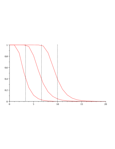
Figure 1: Plot (piecewise linear interpolation) of $\ell\mapsto\mathbb{P}(L(n)\geq\ell)$ for $n=10,100,1000$ and $p=1/2$. The vertical lines are at $\ell=\log_{2}(n)$.

Table 1: Comparing exact and approximate values for $\mathbb{P}(L(n)\geq\ell)$ when $p=1/2$ and $n=10^{4}$

$\ell$	$\mathbb{P}(L(n)\geq\ell)$	$1-\exp(-(n-\ell)p^{\ell}q-p^{\ell})$
10	0.992583894386551	0.992394672192560
12	0.705167040532444	0.704616988848744
14	0.262835671849087	0.262736242068365
20	0.004748524931253	0.004748478671106
50	4.41957581641815 $\times 10^{-12}$	4.42000000000001 $\times 10^{-12}$

Corollary 12 suggests the practical approximation

$$\mathbb{P}(L(n)<\ell)\doteq\exp(-\mathbb{E}G_{\ell}(n))=\exp(-(n-\ell)p^{\ell}q-p^{\ell}),$$ (16)

valid for large $n$ and $\ell$, roughly when $\ell$ is of order $\log_{1/p}n$ or higher. In table 1 we compare the exact result with the approximation for $n=10^{4}$, $p=1/2$, and $\ell$ ranging from slightly below $\log_{2}10^{4}\approx 13.288$ to much higher values. We programmed (15) in Maple to obtain the exact values of $\mathbb{P}(L(n)\geq\ell)$.

In Figure 2 we plot $\ell\mapsto\mathbb{P}(L(n)\geq\ell)$ for $n=1000$ and three different values of $p$. We also plot the analytical approximation given by the right-hand side of (16). Notice that, visually at least, there is no way to tell the difference between real values and the approximating curves.

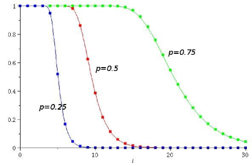
Figure 2: Plot of $\ell\mapsto\mathbb{P}(L(1000)\geq\ell)$ and $p=0.25,0.5,0.75$. The dots correspond to the actual values. The solid lines correspond to the analytical approximation (16)

The result of Lemma 1 easily implies that the law of $G_{\ell(n)}(n)$ converges weakly, as $n\to\infty$ to a Poisson law with mean $\theta$.

Corollary 13.

Under the assumptions of Lemma 1, we have

$$\mathcal{L}\{G_{\ell(n)}(n)\}\to\operatorname{Poisson}(\theta).$$

Proof.

It is enough to establish convergence of binomial moments to those of a Poisson law. Recall that if $N$ is $\operatorname{Poisson}(\theta)$ then $\mathbb{E}\binom{N}{r}=\theta^{r}/r!$. Lemma 1 tells us that the $r$-th binomial moment of $G_{\ell(n)}(n)$ converges to $\theta^{r}/r!$ and this establishes the result. ∎

More interestingly, using the result of Corollary 6, we arrive at

Proposition 2.

Consider $\nu\in\mathbb{N}$, positive real numbers $\theta_{1},\ldots,\theta_{\nu}$, and sequences $\ell_{j}(n)$, $j=1,\ldots,\nu$ of positive integers, such that

$$\lim_{n\to\infty}np^{\ell_{j}(n)}q=\theta_{j},\quad j=1,\ldots,\nu.$$

Then

$$\mathcal{L}\{R_{\ell_{1}(n)}(n),\ldots,R_{\ell_{\nu}(n)}(n)\}\to\operatorname{Poisson}(\theta_{1}q)\times\cdots\times\operatorname{Poisson}(\theta_{\nu}q),$$

as $n\to\infty$.

Proof.

It suffices to show that the joint binomial moments converge to the right thing. Fix $\ell_{1},\ldots,\ell_{\nu}$, $r_{1},\ldots,r_{\nu}$, set $r_{0}=r_{1}+\cdots+r_{\nu}$, and, using the abbreviations (1) for $\alpha,\beta$ and $\gamma$, write the expression (5) for the joint binomial moments as

$$\mathbb{E}\binom{R_{\ell_{1}}^{*}}{r_{1}}\cdots\binom{R_{\ell_{\nu}}^{*}}{r_{\nu}}=(1-w)\,\frac{r_{0}!}{r_{1}!\cdots r_{\nu}!}\,p^{\bm{\ell}\cdot\bm{r}}q^{r_{0}-1}w^{\bm{\ell}\cdot\bm{r}+r_{0}-1}\frac{(1-wp)^{r_{0}+1}}{(1-w)^{r_{0}+1}}$$

Expand $(1-wp)^{r_{0}+1}$ using the binomial formula, and $(1-w)^{r_{0}+1}$ using (6) to write

$$\frac{(1-wp)^{r_{0}+1}}{(1-w)^{r_{0}+1}}=\sum_{k=0}^{\infty}\sum_{s=0}^{r_{0}+1}(-p)^{s}w^{k+s}\binom{r_{0}+1}{s}\binom{r_{0}+k}{r_{0}}$$

and obtain

$$\mathbb{E}\binom{R_{\ell_{1}}^{*}}{r_{1}}\cdots\binom{R_{\ell_{\nu}}^{*}}{r_{\nu}} =(1-w)\,\frac{r_{0}!}{r_{1}!\cdots r_{\nu}!}\,p^{\bm{\ell}\cdot\bm{r}}q^{r_{0}-1}\sum_{k=0}^{\infty}\sum_{s=0}^{r_{0}+1}(-p)^{s}w^{\bm{\ell}\cdot\bm{r}+r_{0}-1+k+s}\binom{r_{0}+1}{s}\binom{r_{0}+k}{r_{0}}$$

$$=(1-w)\,\sum_{n=0}^{\infty}w^{n}\,\sum_{s=0}^{r_{0}+1}\frac{r_{0}!}{r_{1}!\cdots r_{\nu}!}\,p^{\bm{\ell}\cdot\bm{r}}q^{r_{0}-1}(-p)^{s}\binom{r_{0}+1}{s}\binom{n+1-\bm{\ell}\cdot\bm{r}-s}{r_{0}}.$$

Therefore,

$$\mathbb{E}\binom{R_{\ell_{1}}(n)}{r_{1}}\cdots\binom{R_{\ell_{\nu}}(n)}{r_{\nu}} =\frac{r_{0}!}{r_{1}!\cdots r_{\nu}!}\,p^{\bm{\ell}\cdot\bm{r}}q^{r_{0}-1}\sum_{s=0}^{r_{0}+1}(-p)^{s}\binom{r_{0}+1}{s}\binom{n+1-\bm{\ell}\cdot\bm{r}-s}{r_{0}}$$

$$=\frac{q^{-1}}{r_{1}!\cdots r_{\nu}!}\,\sum_{s=0}^{r_{0}+1}(-p)^{s}\binom{r_{0}+1}{s}(n+1-\bm{\ell}\cdot\bm{r}-s)_{r_{0}}\prod_{j=1}^{\nu}(p^{\ell_{j}}q)^{r_{j}},$$

where $(N)_{r_{0}}=N(N-1)\cdots(N-{r_{0}}+1)$. Using the assumptions, we have

$$\lim_{n\to\infty}(n+1-\bm{\ell}\cdot\bm{r}-s)_{r_{0}}\prod_{j=1}^{\nu}(p^{\ell_{j}}q)^{r_{j}}=\theta_{1}^{r_{1}}\cdots\theta_{\nu}^{r_{\nu}},$$

and so

$$\lim_{n\to\infty}\mathbb{E}\binom{R_{\ell_{1}(n)}(n)}{r_{1}}\cdots\binom{R_{\ell_{\nu}(n)}(n)}{r_{\nu}} =q^{-1}\sum_{s=0}^{r_{0}+1}(-p)^{s}\binom{r_{0}+1}{s}\,\frac{\theta_{1}^{r_{1}}}{r_{1}!}\cdots\frac{\theta_{\nu}^{r_{\nu}}}{r_{\nu}!}$$

$$=q^{-1}(1-p)^{r_{0}+1}\,\frac{\theta_{1}^{r_{1}}}{r_{1}!}\cdots\frac{\theta_{\nu}^{r_{\nu}}}{r_{\nu}!}$$

$$=q^{r_{1}+\cdots+r_{\nu}}\,\frac{\theta_{1}^{r_{1}}}{r_{1}!}\cdots\frac{\theta_{\nu}^{r_{\nu}}}{r_{\nu}!},$$

establishing the assertion. ∎

5.2 A better approximation for small length values

We now pass on to a different approximation for $F_{\ell}(n)=\mathbb{P}(L(n)<\ell)$. Consider again (14),

$$\sum_{n=0}^{\infty}w^{n}\,F_{\ell}(n)=\frac{1-(wp)^{\ell}}{1-w+(wq)(wp)^{\ell}},$$ (17)

and look at the denominator

$$f(w):=1-w+p^{\ell}q\,w^{\ell+1},$$

considered as a polynomial in $w\in\mathbb{C}$, of degree $\ell+1$. The smallest (in magnitude) zeros of $f(w)$ govern the behavior of $n\mapsto F_{\ell}(n)$, for $n$ large (and all $\ell$.)

Proposition 3.

The equation

$$f(w)=0,\quad w\in\mathbb{C},$$

has two real roots $w_{0}=w_{0}(\ell)$ and $1/p$, such that

$$1<w_{0}<\frac{\ell+1}{\ell}<\frac{1}{p((\ell+1)q)^{1/\ell}}<\frac{1}{p}, p<\frac{\ell}{\ell+1}$$

$$1<\frac{1}{p}<\frac{\ell+1}{\ell}<\frac{1}{p((\ell+1)q)^{1/\ell}}<w_{0}, p>\frac{\ell}{\ell+1}$$

$$1<w_{0}=\frac{1}{p}, p=\frac{\ell}{\ell+1},$$

and all other roots are outside the circle with radius $\max(w_{0},1/p)$ in the complex plane. Moreover, $\lim_{\ell\to\infty}w_{0}(\ell)=1$.

Proof.

We check the behavior of $f(w)$ for real $w$. First, we have $f(1/p)=0$. Now, $f^{\prime}(w)=-1+(\ell+1)p^{\ell}qw^{\ell}$, and so the only real root of $f^{\prime}(w)=0$ is $w^{*}=1/p((\ell+1)q)^{1/\ell}$. Since $f^{\prime\prime}(w)=\ell(\ell+1)p^{\ell}qw^{\ell-1}$, the function $f$ is strictly convex on $[0,\infty)$ and so $f(w^{*})$ is a global minimum of $f$ on $[0,\infty)$. Notice that $f(w^{*})=1-\ell w^{*}/(\ell+1)$. We claim that $f(w^{*})\leq 0$, or, equivalently, that $w^{*}\geq(\ell+1)/\ell$. Upon substituting with the value of $w^{*}$, this last inequality is equivalent to $p^{\ell}(1-p)\leq(\ell/(\ell+1))^{\ell}$. But this is true, since $\max_{0\leq p\leq 1}p^{\ell}(1-p)=\ell^{\ell}/(\ell+1))^{\ell+1}\leq(\ell/(\ell+1)^{\ell})$. Hence $f(w^{*})\leq 0$ with equality if and only if $p=\ell/(\ell+1)$. On the other hand, $f(0)=1$ and $\lim_{w\to\infty}f(w)=\infty$. Therefore $f(w)=0$ has two positive real roots straddling $w^{*}$. One of them is $1/p$. Denote the other root by $w_{0}$. Since $f((\ell+1)/\ell)=-\frac{1}{\ell}+((\ell+1)/\ell)^{\ell+1}p^{\ell}q<0$, and $f(w^{*})<0$, provided that $p\neq\ell/(\ell+1)$, it actually follows that, in this case, $w_{0}$ and $1/p$ are outside the interval $[(\ell+1)/\ell,\,w^{*}]$. Depending on whether $p$ is smaller or larger than $\ell/(\ell+1)$, we have $w_{0}<1/p$ or $w_{0}>1/p$, respectively. If $p=\ell(\ell+1)$ then $w^{*}=(\ell+1)/\ell$ and then $1/p=w_{0}=w^{*}$. Since $f(1)=p^{\ell}q$, it follows that $w_{0}>1$, in all cases. Finally, for all sufficiently large $\ell$, we have $p<\ell/(\ell+1)$ and so $1<w_{0}<(\ell+1)/\ell$, showing that the limit of $w_{0}$, as $\ell\to\infty$, is $1$. To show that the only roots $f(w)=0$ with $|w|\leq\max(w_{0},1/p)$ are $w_{0}$ and $1/p$, we need an auxiliary lemma which is probably well-known but whose proof we supply for completeness:

Lemma 2.

Consider the polynomial $P(z):=c_{0}+c_{1}z+\cdots+c_{n}z^{n}$, $z\in\mathbb{C}$, with real coefficients such that $c_{0}>c_{1}>\cdots>c_{n}>0$. Then all the zeros of $P(z)$ lie outside the closed unit ball centered at the origin.

Proof.

Fix $\lambda>1$ such that $c_{0}>c_{1}/\lambda>c_{2}/\lambda^{2}>\cdots>c_{n}/\lambda^{n}$ and notice that

$$c_{0}+(z-1)\,P(z/\lambda)=(c_{0}-\frac{c_{1}}{\lambda})z+(\frac{c_{1}}{\lambda}-\frac{c_{2}}{\lambda^{2}})z^{2}+\cdots+(\frac{c_{n-1}}{\lambda^{n-1}}-\frac{c_{n}}{\lambda^{n}})z^{n}+\frac{c_{n}}{\lambda^{n}}z^{n+1}.$$

Therefore, on $|z|=1$,

$$\big{|}c_{0}+(z-1)\,P(z/\lambda)\big{|}\leq(c_{0}-\frac{c_{1}}{\lambda})+(\frac{c_{1}}{\lambda}-\frac{c_{2}}{\lambda^{2}})+\cdots+(\frac{c_{n-1}}{\lambda^{n-1}}-\frac{c_{n}}{\lambda^{n}})+\frac{c_{n}}{\lambda^{n}}=c_{0}=|-c_{0}|.$$

Rouché’s theorem [1, page 153] implies that $(z-1)\,P(z/\lambda)$ and $-c_{0}$ have the same number of zeros inside the open unit ball centered at the origin. That is, all zeros of $P(z/\lambda)$ lie outside the open unit ball. Since $\lambda>1$, it follows that all zeros of $P(z)$ lie outside the closed unit ball. ∎

End of proof of Proposition 3.

Assume first $w_{0}p\neq 1$. By polynomial division, write $f(w)$ as

$$f(w)=-q(1-pw)(w-w_{0})S(w),$$

where

$$S(w):=\sum_{j=0}^{\ell-1}\frac{1-(w_{0}p)^{\ell-j}}{1-w_{0}p}\,p^{j}w^{j}.$$

Since the positive numbers $(1-(w_{0}p)^{\ell-j})/(1-w_{0}p)$ decrease with $j$, it follows from Lemma 2 that if $S(w)=0$ then $|pw|>1$, i.e., $|w|>1/p$. On the other hand, since $S(w)=\sum_{j=0}^{\ell-1}(1-(w_{0}p)^{\ell-j})(w_{0}p)^{j}/(1-w_{0}p)\,(w/w_{0})^{j}$ and since the positive numbers $(1-(w_{0}p)^{\ell-j})(w_{0}p)^{j}/(1-w_{0}p)$ decrease with $j$ it follows again by Lemma 2 that $S(w)=0$ implies $|w/w_{0}|>1$, i.e., $|w|>w_{0}$. If $w_{0}p=1$ then $S(w)=\sum_{j=0}^{\ell-1}(\ell-j)p^{j}w_{j}$ and so $S(w)=0$ implies $|w|>1/p=w_{0}$. ∎

We translate this result into an approximation for the distribution function of $L(n)$.

Proposition 4.

Let $w_{0}=w_{0}(\ell)$ be the root of the equation $f(w)=0$ defined in Proposition 3. If $p\neq\ell/(\ell+1)$ then

$$\mathbb{P}(L(n)<\ell)\sim\frac{1-(w_{0}p)^{\ell}}{1-(\ell+1)q(w_{0}p)^{\ell}}\,w_{0}^{-n-1},\text{ as }n\to\infty.$$

If $p=\ell/(\ell+1)$ then

$$\mathbb{P}(L(n)<\ell)\sim 2(\ell/(\ell+1))^{n+1},\text{ as }n\to\infty.$$

Proof.

Suppose first that $p\neq\ell/(\ell+1)$ and, using partial fraction expansion, write the expression (17) as

$$\frac{g(w)}{f(w)}=\frac{1-(wp)^{\ell}}{1-w+(wq)(wp)^{\ell}}=\frac{c_{0}}{1-w/w_{0}}+\frac{h(w)}{j(w)}.$$ (18)

To do this, we use the fact that $w_{0}$ is a zero of the denominator $f(w)=1-w+(wq)(wp)^{\ell}$ but not a zero of the numerator $g(w)=1-(wp)^{\ell}$. Also, $w_{0}\neq 1/p$, and both $g(w)$ and $f(w)$ have a zero at $1/p$. Hence $h(w)$ and $j(w)$ are polynomials with degrees $\ell-2$ and $\ell-1$, respectively, and $j(w_{0})\neq 0$. Hence

$$c_{0}=\frac{1}{w_{0}}\,\lim_{w\to w_{0}}\frac{(w_{0}-w)g(w)}{f(w)}=\frac{g(w_{0})}{-f^{\prime}(w_{0})}\,\frac{1}{w_{0}}=\frac{1-(w_{0}p)^{\ell}}{1-(\ell+1)q(w_{0}p)^{\ell}}\,\frac{1}{w_{0}}.$$

Proposition 3 tells us that the zeros of $j(w)$ are all outside the circle with radius $w_{0}$. Hence, from expressions (18) and (17), we obtain

$$\mathbb{P}(L(n)<\ell)\sim c_{0}\,w_{0}^{-n},\text{ as }n\to\infty,$$ (19)

which proves the first assertion. If $p=\ell/(\ell+1)$ then $w=1/p=w_{0}$ is a simple zero for $g(w)$ and a double zero for $f(w)$. Hence (18) gives

$$c_{0}=-\frac{g^{\prime}(w_{0})}{\frac{1}{2}f^{\prime\prime}(w_{0})}\,\frac{1}{w_{0}}=\frac{-p^{\ell}qw_{0}^{\ell-1}}{\frac{1}{2}p^{\ell}q\ell(\ell+1)w_{0}^{\ell-1}}\,\frac{1}{w_{0}}=\frac{2}{q(\ell+1)w_{0}}=\frac{2\ell}{\ell+1}.$$

Since the zeros of $j(w)$ are outside the circle with radius $w_{0}=(\ell+1)/\ell$, (19) holds. This proves the second assertion. ∎

Since these approximations are valid for all $\ell$, they nicely complement the Poisson approximation discussed earlier. For $n,\ell\to\infty$, such that $np^{\ell}\asymp 1$, we have $w_{0}(\ell)=1+p^{\ell}q+O(\ell/n^{2})$. From the approximation above, we find $\mathbb{P}(L_{\ell}(n)<\ell)\approx e^{-np^{\ell}q}$ which is asymptotically equivalent to the Poisson approximation.

5.3 Numerical comparisons of the two approximations

We numerically compute $\mathbb{P}(L(n)\geq\ell)$, first using the exact formula (15), then using the Poisson approximation (16), and finally using the approximation suggested by Proposition 4. We see, as expected, that for small values of $\ell$ compared to $n$, the second approximation outperforms the first one.

First, we let $\ell=2$. Then $f(w)=1-w+p^{2}qw^{3}=(pw-1)(pqw^{2}+qw-1)$, and so

$$w_{0}=\frac{\sqrt{1+4p/q}-1}{2p}.$$

The approximation suggested by Proposition 4 is

$$\mathbb{P}(L(n)<2)\sim\begin{cases}\displaystyle\frac{1-(w_{0}p)^{2}}{1-3q(w_{0}p)^{2}}\,w_{0}^{-n+1},&\text{ if }p\neq 2/3,\\ 2(2/3)^{-(n+1)},&\text{ if }p=2/3\end{cases}$$

Below are some numerical values.

$\mathbb{P}(L(n)\geq\ell)$ for $p=1/2$ and $\ell=2$
$n$	exact	Poisson approx. (error)	second approx. (error)
5	0.59375	0.46474 (22%)	0.59426 (0.086%)
7	0.73438	0.58314 (20.6%)	0.73445 (0.01%)
10	0.85938	0.71350 (17%)	0.8594 (0.002%)
20	0.98311	0.91792 (6.63%)	0.98312 (0.0010%)

$\mathbb{P}(L(n)\geq\ell)$ for $p=1/3$ and $\ell=2$
$n$	exact	Poisson approx. (error)	second approx. (error)
5	0.32510	0.28347 (12.8%)	0.32557 (0.14%)
7	0.44033	0.38213 (13.2%)	0.44080 (0.11%)
10	0.57730	0.50525 (12.5%)	0.57779 (0.08%)
20	0.83415	0.76411 (8.4%)	0.83453 (0.05%)

$\mathbb{P}(L(n)\geq\ell)$ for $p=4/5$ and $\ell=2$
$n$	exact	Poisson approx. (error)	second approx. (error)
5	0.94208	0.64084 (32.0%)	0.94386 (0.189%)
7	0.98509	0.72196 (26.71%)	0.98526 (0.0173%)
10	0.9980232	0.8106201 (18.78%)	0.9980179 (0.00052%)
20	0.9999975	0.9473453 (5.265%)	0.9999975 ($0.000003$%)

Next, we increase the value of $\ell$ and pick two different values for $p$. We solve, in each case, the equation $f(w)=0$ numerically.

$\mathbb{P}(L(n)\geq\ell)$ for $p=1/2$ and $\ell=7$
$n$	exact	Poisson approx. (error)	second approx. (error)
100	0.31752	0.31002 (2.36%)	0.19644 (38.13%)
500	0.86364	0.85537 (0.96%)	0.8372 (3.06%)
1500	0.99757	0.99709 (0.048%)	0.99700 (0/057%)
3000	0.9999941986	0.9999916997 (0.00025%)	0.9999931928 (0.00010%)

$\mathbb{P}(L(n)\geq\ell)$ for $p=2/3$ and $\ell=10$
$n$	exact	Poisson approx. (error)	second approx. (error)
100	0.43531	0.41583 (4.475%)	0.46433 (6.667%)
500	0.95209	0.94214 (1.045%)	0.95480 (0.285%)
1500	0.999900	0.999821 (0.00790%)	0.999905 (0.00050%)
3000	0.9999999904	0.9999999694 (2.1$\times 10^{-6}$%)	0.9999999908 (0.04 $\times 10^{-6}$%)

6 Discussion and open problems

Gordon, Schilling and Waterman [8] developed an extreme value theory for long runs. As mentioned therein, it is intriguing that the longest run possesses no limit distribution, and this is based on an older paper by Guibas and Odlyzko [9].

We have not touched upon the issue of more general processes generating heads and tails. For example, Markovian processes. The portmanteau identity can be generalized to include the Markovian dependence and this can be the subject for future work provided that a suitable motivation be found.

Another set of natural questions arising is to what extent we have weak approximation of $R(n)$ on a function space (convergence to a Brownian bridge?), as well as the quality of such an approximation.

Acknowledgments

We would like to thank Joe Higgins for the short proof of Lemma 2.

Lars Holst
Department of Mathematics
Royal Institute of Technology
SE-10044 Stockholm
Sweden
Email: lholst@kth.se

Takis Konstantopoulos
Department of Mathematics
Uppsala University
SE-75106 Uppsala
Sweden
E-mail: takis@math.uu.se

References

- [1] L. V. Ahlfors (1979). Complex Analysis. Mc-Graw Hill, New York.
- [2] N. Balakrishnan and M. Koutras (2002). Runs and Scans with Applications. Wiley, New York.
- [3] P. Erdős and A. Rényi (1970). On a new law of large numbers. J. Analyse Math. 22, 103-111.
- [4] P. Erdős and P. Révész (1976). On the length of the longest headrun. Topics in Information Theory (Second Colloq., Keszthely, 1975), pp. 219-228. Colloq. Math. Soc. János Bolyai, Vol. 16, North-Holland, Amsterdam, 1977.
- [5] W. Feller (1968). An Introduction to Probability Theory and its Applications, Vol. I. Third edition, John Wiley, New York.
- [6] J.C. Fu and W.Y.W. Lou (2003). Distribution Theory of Runs and Patterns and its Applications. World Scientific, River Edge, NJ.
- [7] G. Grimmett and D. Stirzaker (2001). Probability and Random Processes, 3d Ed. Oxford University Press, Oxford.
- [8] L. Gordon, M.F. Schilling and M.S. Waterman (1986). An extreme value theory for long head runs. Probab. Theory Relat. Fields 72, 279-287.
- [9] L.J. Guibas and A.M. Odlyzko (1980). Long repetitive patterns in random sequences. Z. Wahrsch. verw. Gebiete bf 53, 241-262.
- [10] R.L. Graham, D.E. Knuth and O. Patashnik (1994). Concrete Mathematics. Addison-Wesley, Reading, Massachusetts.
- [11] F.S. Makri and Z.M. Psillakis (2011). On success runs of length exceeded a threshold. Methodol. Comput. Appl. Probab. 13, 269-305.
- [12] D.B. Murray and S.W. Scott (1993). Probability of a tossed coin landing on edge. Physical Review E (Statistical Physics, Plasmas, Fluids, and Related Interdisciplinary Topics), 48, 2547-2552.
- [13] M. Muselli (1996). Simple expressions for success run distributions in Bernoulli trials. Stat. Probab. Lett. 31, 121-128.
- [14] A. Philippou and F.S. Makri (1986). Success runs and longest runs. Stat. Prob. Letters, 4, 101-105.
- [15] P. Révész (1980). Strong theorems on coin tossing. Proc. International Congress of Mathematicians (Helsinki, 1978), pp. 749-754, Acad. Sci. Fennica, Helsinki.
- [16] R. von Mises (1921). Zur Theorie der Iterationen. Zeitschr. für angew. Mathem. und Mechan. 1, 298-307.
- [17] R. von Mises (1981). Probability, Statistics and Truth. Dover, New York. (Originally published in German in 1928; this is a translation from the third 1957 German edition.)