Valence Bond Phases in $S=1/2$ Kane-Mele-Heisenberg Model

Abstract

The phase diagram of Kane-Mele-Heisenberg (KMH) model in classical limit zare , contains disordered regions in the coupling space, as the result of to competition among different terms in the Hamiltonian, leading to frustration in finding a unique ground state. In this work we explore the nature of these phase in the quantum limit, for a $S=1/2$. Employing exact diagonalization (ED) in $S_{z}$ and nearest neighbor valence bond (NNVB) bases, bond and plaquette valence bond mean field theories, We show that the disordered regions are divided into ordered quantum states in the form of plaquette valence bond crystal (PVBC) and staggered dimerized (SD) phases.

I Introduction

Two-dimensional frustrated spin systems with $S=1/2$ have lately received massive attentions, due to their potential for realizing the quantum spin liquid (QSL), a magnetically disordered state which respects all the symmetries of the systems, even at absolute zero temperature balent . The spin model, recently attracted many interests, is the Heisenberg model with first and second anti-ferromagnetic exchange interaction, the $J_{1}-J_{2}$ model, in honeycomb lattice. The lowest coordination number ($z=3$) in 2D, being the unique peculiarity of honeycomb, makes this lattice a promising candidate to host QSL. It is known that the classical $J_{1}-J_{2}$ model do not show any long range ordering at $T=0$ for $\frac{1}{6}<\frac{J_{2}}{J_{1}}<0.5$, because of high degeneracy in the energy of ground state fouet . However, thermal fluctuations are able to lower the free energy of some specific spiral states within the ground state manifold kawamura , a phenomenon called thermal order by disorder villain . So far, many efforts have been devoted to gain insight into the quantum nature of this disordered region for $S=1/2$ systems. Some of these works support the existence of QSL qsl1 ; qsl2 ; qsl3 ; qsl4 ; qsl5 ; qsl6 for $0.2\lesssim\frac{J_{2}}{J_{1}}\lesssim 0.5$, while others suggest a translational broken symmetry state with plaquette valence bond ordering for $0.2\lesssim\frac{J_{2}}{J_{1}}\lesssim 0.35$ which transforms to a nematic staggered dimerised state when the ratio $\frac{J_{2}}{J_{1}}$ rises to lay within $0.35\lesssim\frac{J_{2}}{J_{1}}\lesssim 0.5$ aron2010 ; mosadeq ; pvb2 ; pvb3 ; pvb4 ; pvb5 ; pvb6 ; pvb7 . For $\frac{J_{2}}{J_{1}}>0.5$, a long ranged collinear ordered ground state is proposedpvb2 ; pvb7 .

Quick progresses in the filed of topological insulators (TI) Kane2005 ; Kane20051 ; top4 ; top5 ; top6 ; top1 ; top2 ; top3 , has drawn the attention of the physicists into the study of the effective spin models in the strong coupling limit of TI models. Kane-Mele-Hubbard model, is an example of such models which recently has been studied by various methods kmh1 ; kmh2 ; kmh3 ; kmh4 ; kmh5 ; kmh6 ; kmh7 ; kmh8 ; kmh9 ; kmh10 ; kmh11 ; kmh12 ; kmh13 ; kmh14 ; kmh15 ; kmh16 ; kmh17 ; kmh18 ; kmh19 ; kmh20 . The strong coupling (large Coulomb interaction) and weak coupling (small Coulomb interaction) limits of this model are charachterized by anti-ferromagnetic Mott insulator (AFMI) and topological band insulator (TBI) phases, respectively. For intermediate Coulomb interactions and weak spin-orbit coupling a gapped QSL phase has been proposed for his model kmh10 .

The strong coupling limit of Kane-Mele-Hubbard model is effectively described by a XXZ model, also called Kane-Mele-Heisenberg(KMH) model kmh1 . Classical phase diagram of KMH model contains six regions in the coupling space zare . In the three regions the model is long-range ordered, planar Néel state in honeycomb plane (phase I), commensurate spiral states in the plan normal to honeycomb lattice (phase VI) and collinear states along perpendicular to honeycomb plane (phase II). In the other three regions the system is disordered, the ground state is infinitely degenerate and characterized by a manifold of incommensurate wave-vectors. These phases are, planar spiral (phase III), vertical spiral states (phase IV) and non-coplanar states (phase V). Apart from a Schwinger boson and Schwinger fermion study vaezi , where a chiral spin liquid state is proposed for a narrow region but large values of second neighbor exchange interaction ($J_{2}$), the quantum phase diagram of KMH model has remain unexplored.

Our aim in this work, is understanding the nature of the quantum ground state of $S=1/2$ KMH model for intermediate values of $J_{2}$, mostly in phases III and IV, where it is classically disordered. For this purpose, we use exact diagonalization as well as valence bond and plaquette mean field theories.

The paper is organized as follows. In Sec. II the KMH model is introduced. The quantum ground state properties of the classically disordered phases are investigated, using ED for a finite lattice in Sec. III and bond operator and plaquette valence bond mean field theories in Sec. IV. Section V is devoted to conclusion. The details of bond operator and plaquette mean field theories are given in appendices A and B, respectively.

II Model Hamiltonian

Kane-Mele-Hubbard model is described by the following Hamiltonain

$$H=-t\sum_{\langle ij\rangle,\sigma}c_{i\alpha}^{\dagger}c_{j\alpha}+i\lambda\sum_{\langle\!\langle i,j\rangle\!\rangle,\alpha\beta}\nu_{ij}\sigma_{\alpha\beta}^{z}c_{i\alpha}^{\dagger}c_{j\beta}+\sum_{i}Un_{i\uparrow}n_{i\downarrow},$$ (1)

in which $\langle\cdots\rangle$ and $\langle\!\langle\cdots\rangle\!\rangle$ denote the nearest and next to nearest neighbor sites in a honeycomb lattice. First term represents the hopping between nearest neighbor atoms, while the second term , with $\nu_{ij}=\pm 1$ being an anti-symmetric tensor, denotes the hopping between the second neighbors arising from the spin-orbit coupling. The last term is onsite Hubbard term, in which $U>0$ denotes the Coulomb repulsion energy between two electrons within a single atom. In strong coupling limit, where $U$ is much larger than $t$ and $\lambda$, the model can be effectively described by a $S=1/2$ spin Hamiltonain, namely the Kane-Mele-Heisenberg ( KMH ) model kmh1

$$\begin{split}H_{\rm KMH}\!\!&=\!\!J_{1}\sum_{\langle i,j\rangle}{\bf S}_{i}\cdot{\bf S}_{j}+J_{2}\sum_{\langle\!\langle i,j\rangle\!\rangle}{\bf S}_{i}\cdot{\bf S}_{j}\\ &+g_{2}\sum_{\langle\!\langle i,j\rangle\!\rangle}(-S_{i}^{x}~{}S_{j}^{x}-S_{i}^{y}~{}S_{j}^{y}+S_{i}^{z}~{}S_{j}^{z}),\end{split}$$ (2)

in which $J_{1}=4t^{2}/U-16{t^{4}}/U^{3}$, $J_{2}=4{t^{4}}/U^{3}$ and $g_{2}=4{\lambda^{2}}/U$ are the first and second neighbor exchange couplings.

III Exact diagonalizaion

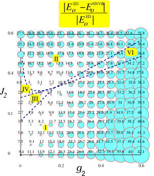
Figure 1: (Color online) Relative difference between the ground-state energy obtained by diagonalization in NNVB basis ($E_{0}^{\rm NNVB}$) and $S_{z}$ basis ($E_{0}^{\rm ED}$) in coupling space $g_{2}-J_{2}$, for $N=24$ lattice points and $J_{1}=1$. Dashed lines display the phase boundaries of the classical KMH model. The radii of the circles are proportional to the relative error, represented in percentage.

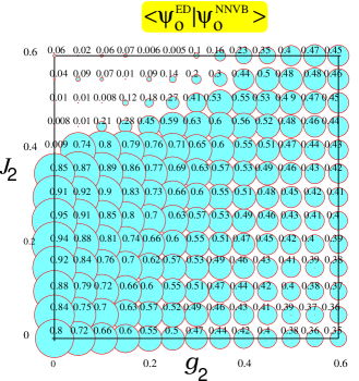
Figure 2: (Color online) Overlap between normalized ground state wave functions, obtained by diagonalization in NNVB basis ($\psi_{0}^{\rm NNVB}$) and $S_{z}$ basis ($\psi_{0}^{\rm ED}$) in $g_{2}-J_{2}$, for $N=24$ lattice points and $J_{1}=1$. The radii of the circles are proportional to the magnitude of the overlaps.

To gain insight into the fate of the classically disordered region of ${\rm KMH}$ model in the quantum limit, we employ the exact diagonalization method in both $S_{z}$ and nearest neighbor valence bond (NNVB) bases. NNVB, a basis composed of the products of nearest neighbor singlet paris of $S=1/2$ spins, provides a natural framework for characterising the features of the disordered quantum ground states.The spin disordered states such as resonating valence bond (RVB) spin liquid and plaquette valence bond crystal (PVBC) receive most of their components from the the Hilbert space spanning only by NNVB basis. Therefore, comparing the results of ED within $S_{z}$ with those obtained by NNVB basis, would be a guideline to learn about the nature of the ground state in classically degenerated phases III and IV.

Let us expand the ground state wave function in terms of NNVB states as

$$|\psi_{0}\rangle=\sum_{\alpha}a(c_{\alpha})|c_{\alpha}\rangle,$$ (3)

where $|c_{\alpha}\rangle$ denotes all possible configurations $\alpha$ of NNVBs:

$$|c_{\alpha}\rangle=\prod_{(i,j)\in\alpha}(i_{\uparrow}j_{\downarrow}-i_{\downarrow}j_{\uparrow}).$$ (4)

First, we have to enumerate the basis $|c_{\alpha}\rangle$ to construct a numerical representation of the Hamiltonian matrix in this basis. To determine the basis, the exact Pfaffian representation of the RVB wave function is employed emrrvb . In this method one expresses the RVB wave function as the Pfaffian of an antisymmetric matrix whose dimension is equal to the number of the lattice points. The dimension of Hilbert space corresponding to NNVB basis is much smaller than the one for whole $S_{z}=0$ basis, so that the Hamiltonian matrix can be fully diagonalized with standard library routines. Note that since the NNVB components ($|c_{\alpha}\rangle$) are not orthonormal, one needs to solve the generalized eigen-value problem

$$\det[{\cal H}-E{\cal O}]=0,$$

where ${\cal O}=\langle c_{\beta}|c_{\alpha}\rangle$ denotes the overlap matrix between different NNVB configurations.

We begin with calculation of relative error in ground state energy between exact and NNVB basis, $(E_{0}^{\rm NNVB}-E_{0}^{\rm ED})/{E_{0}^{\rm ED}}$ and also the overlap of the corresponding ground state wave functions. From now on we set $J_{1}=1$. Figs.1 and 2 show the relative errors (in percent) and the overlapping of the ground state wave functions, respectively, for a system consisting of $N=24$ lattice points. Relative errors and wave function overlaps indicate that the best match between the ground states, obtained by the two bases, occurs mostly in classically disordered Phase.III and also large part of the phase. IV.

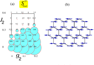
Figure 3: (Color online) Structure function of planar Néel, calculated by exact diagonalization in $S_{z}$ basis for $N=24$ lattice points. The radii of the circles are proportional to the magnitude of the structure function (magnified by the factor 1000) for each point in the coupling space. (b) Schematic representation of Néel-$xy$ state, proposed for phase.I.

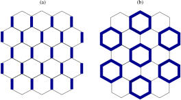
Figure 4: (Color online) Schematic representaion of (a) Staggered dimerized (SD), and (b) Plaquette valence bond crystal (PVBC).

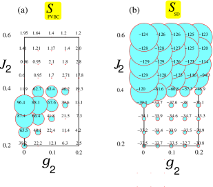
Figure 5: (Color online) (a) Plaquette valence bond crystal, and (b) Staggered dimerized structure functions, calculated by exact diagonalization in $S_{z}$ basis for $N=24$ lattice points. The radii of the circles are proportional to the magnitude of the structure function (magnified by the factor 1000) calculated for each point in the coupling space.

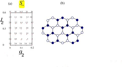
Figure 6: (Color online) (a) Structure function of the collinear state along $z$-axis, calculated by exact diagonalization in $S_{z}$ basis for $N=24$ lattice points. The radii of the circles are proportional to the magnitude of the structure function (magnified by the factor 1000) for each point in the coupling space. (b) Schematic representation of collinear-$z$ state, proposed for phase II in classical limit. Black and white circles denote the up and down spins, respectively.

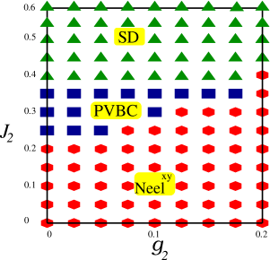
Figure 7: (Color online) Quantum phase diagram obtained from exact diagonalization for a finite lattice with $N=24$.

Now we proceed to inspect the possible orderings in the coupling space by defining appropriate structure functions. Since the spin-orbit coupling is small for real materials, we limit ourselves to $0<g_{2}<0.2$ and $0<J_{2}<0.6$. For small values of $J_{2}$, the classical ground state is planar Néel state. To investigate the region in coupling space where this ordering is extended, we calculate a structure function corresponding to it in terms of spin-spin correlation functions as

$$S_{\rm Neel}^{xy}=\frac{1}{N^{2}} (\sum_{i,j\in A{\rm or}B}\langle S_{i}^{x}S_{j}^{x}+S_{i}^{y}S_{j}^{y}\rangle-$$ (5)

$$\sum_{i\in A,j\in B}\langle S_{i}^{x}S_{j}^{x}+S_{i}^{y}S_{j}^{y}\rangle),$$

in which $N$ is the number of lattice points and $A,B$ denote the two sublattices of honeycomb.

The obtained structure function for Néel-$xy$ is depicted in Fig 3, indicating that the Néel ordering in honeycomb plane extends to $J_{2}\sim 0.2$ for $g_{2}=0$ and stretches up to $J_{2}\sim 0.3$ as $g_{2}$ tends to $0.2$.

Now we seek the features of the disordered quantum ground state, where Néel ordering vanishes, and see whether they break any symmetries of the lattice. The proposed $SU(2)$ symmetric ground states, breaking the symmetries of honeycomb lattice, are the staggered dimerized (SD) or nematic valence bond solid, which breaks the $C_{3}$ rotational symmetry and plaquette valence bond crystal (PVBC) which breaks the translational symmetry of the honeycomb lattice (Fig.4). The structure functions for SD and PVBC can be defined in terms of dimer-dimer correlations as

$$S_{\lambda}=\frac{1}{N_{b}}\sum_{\alpha^{\prime}}\varepsilon_{\lambda}(\alpha^{\prime})~{}C(\alpha,\alpha^{\prime}),$$ (6)

where $N_{b}$ denotes the number of bonds and $C(\alpha,\alpha^{\prime})$ is the dimer-dimer correlation given by

$$C(\alpha,\alpha^{\prime})=4(\langle(\textbf{S}_{i}.\textbf{S}_{j})(\textbf{S}_{k}.\textbf{S}_{l})\rangle-{\langle(\textbf{S}_{i}.\textbf{S}_{j})\rangle}^{2}),$$ (7)

where $\alpha^{\prime}=(k,l)$, and $\alpha=(i,j)$ denotes the reference bond relative to which the correlations are calculated. $\varepsilon_{\lambda}(\alpha^{\prime})$ is the phase factor, appropriately defined for each of the two states $\lambda\equiv$SD, PVBC mambrini .

The two structure functions, calculated exactly in $S_{z}$ basis for $N=24$, are represented in Fig. 5, where the radii of the circles denote the strength of aforementioned orderings for each set of couplings $(g_{2},J_{2})$. Fig. 5-a shows that in the most part of phases III and IV, where the ground state is well described by NNVB basis, the PVBC structure function is remarkably large, while for $J_{2}\gtrsim 0.4$, it falls down abruptly. On the other hand, Fig 5-b shows the sudden growth of SD structure function for $J_{2}\gtrsim 0.4$, the indication of first order phase transition between PVBC and SD states. As can also be seen from this figure, for the range of coupling under study, the SD ordering is well developed inside the phase II, for which a collinear ordering perpendicular to the honeycomb plane is found in classical limit. The structure function corresponding to collinear-$z$ ordering, for which a possible configuration is depicted in Fig 6-b, can be defined as

$$S_{{\rm COL}}^{z}=\frac{1}{N^{2}}\sum_{i,j}e^{i[{\bf q}.({\bf r}_{i}-{\bf r}_{j})]}\langle S_{i}^{z}S_{j}^{z}\rangle,$$ (8)

in which ${\bf q}=(\pi,\pi/\sqrt{3})$, ${\bf r}_{i}$ denotes the translational vector of triangular Bravais lattice and the unit cell is chosen in such a way to contain two parallel spins. Fig 6-a displays the values of $S_{\rm COL}^{z}$ obtained from ED calculation. The magnitudes of this structure function, being very small compare to the ones corresponding to SD ordering, verify the alternation of SD ordering instead of collinear-$z$ state in phase II, at least for $g_{2}<0.2$.

The results of this section is summarized in a finite lattice quantum phase diagram, represented in Fig. 7.

IV Bond Operator Method

Inspired by ED calculation on the finite system, in this section we employ bond operator as well as plaquette operator mean-field theories to investigate the regions of the stability of PVBC and SD phases and transition between them, for the infinite lattice.

The bond operator formalism is introduced by Chubokov chubukov and Sachdev and Bhatt sachdev , for describing the disordered phases of a frustrated spin Hamiltonian. In this formalism, a couple of $S=1/2$ spin operators belonging to a bond are represented in terms of the components of their summation, with a Hilbert space consisting of one singlet $|s\rangle$ and three triplet states $|t_{x}\rangle$, $|t_{y}\rangle$ and $|t_{z}\rangle$. Introducing, the singlet and triplet creation operators out of vacuum $|0\rangle$

$$|s\rangle = s^{{\dagger}}|0\rangle=\frac{1}{\sqrt{2}}(|\uparrow\downarrow\rangle-|\downarrow\uparrow\rangle)$$

$$|t_{x}\rangle = {t_{x}}^{{\dagger}}|0\rangle=\frac{-1}{\sqrt{2}}(|\uparrow\uparrow\rangle-|\downarrow\downarrow\rangle)$$

$$|t_{y}\rangle = {t_{y}}^{{\dagger}}|0\rangle=\frac{i}{\sqrt{2}}(|\uparrow\uparrow\rangle+|\downarrow\downarrow\rangle)$$

$$|t_{z}\rangle = {t_{z}}^{{\dagger}}|0\rangle=\frac{1}{\sqrt{2}}(|\uparrow\downarrow\rangle+|\downarrow\uparrow\rangle),$$

one can express a spin residing on site $n$, in terms of these basis states as ${\bf S}_{n}=\sum_{\mu,\nu}|\mu\rangle\langle\mu|{\bf S}_{n}|\nu\rangle\langle\nu|$. Here $|\mu\rangle$ and $|\nu\rangle$ can be each of the above four states. Evaluation of the matrix elements $\langle\mu|{\bf S}_{n}|\nu\rangle$, gives rise to the representation of the spin operator in terms of the bosonic bond operators

$$S_{n}^{\alpha}=\frac{{(-1)}^{n}}{2}(s^{{\dagger}}t_{\alpha}+t_{\alpha}^{{\dagger}}s)-\frac{i}{2}{\epsilon}_{\alpha\beta\gamma}t_{\beta}^{{\dagger}}{t_{\gamma}},$$ (10)

where $\alpha$, $\beta$ and $\gamma$ stand for $x$,$y$ and $z$ and $\epsilon$ is the totally anti-symmetric tensor. Moreover, the fact that each bond is either in a singlet or triplet state, leads to the following constraint

$$s^{{\dagger}}s+\sum_{\alpha}{t_{\alpha}}^{{\dagger}}{t_{\alpha}}=1$$ (11)

Now, considering a SD configuration illustrated in Fig. 4-a, the spin Hamiltonian 2 can be decomposed into the inter and intra bond terms given by Eq. 16. Using the spin representations 10, we achieve a bosonic Hamiltonian in terms of singlet and triplet operators, in which all the singlets are considered to be condensed. Then, keeping only the quadratic triplet terms, as an approximation, enables us to diagonalize the resulting Hamiltonian by the use of Bogoliubov transformations. Finally, minimization of the total energy subjected to the constraint 11, provides us with a set of self consisted equations. Numerical solution of these equations gives the energy of corresponding dimerized configuration. The details of the derivation of self-consisted equations are given in appendix A.

In order to find the energy of a plaquette ordered state, we rewrite the spin Hamiltonian 2 in terms of the plaquette operators defining based on the eigenstates of KMH Hamiltonain for a single hexagon. In the absence of Kane-Mele term, i.e $g_{2}=0$, The commutation relation $[H,{\bf S}^{2}]=0$, enables us to label each eigenstate of such a Hamiltonian by the eigenvalues of ${\bf S}^{2}$ operator. The ground state is then found to be a spin singlet, invariant under rotation by $60^{0}$, up to $J_{2}/J_{1}=$0.5. This ground state is predominantly expressed by the symmetric combination of two Kekule structures, implying that the ground state of $J_{1}-J_{2}$ within a hexagon is s-wave singlet, in contrast to the f-wave singlet (the anti-symmetric superposition of two Kekule structures) proposed in pvb5 . The first excited states are also found to be triplet for $0<J_{2}/J_{1}<0.25$ and replaced by a f-wave singlet state for $J_{2}/J_{1}>0.25$.

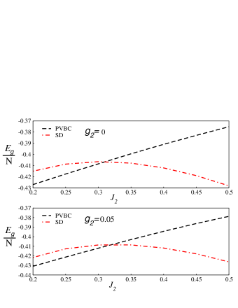
Figure 8: (Color online) The ground state energy per spin obtained from bond operator method for SD state (dotted-dashed line) and from plaquette operator method for PVBC state ( dashed line) versus $J_{2}$ for (top) $g_{2}=0.0$ and (bottom) $g_{2}=0.05$.

Now, we proceed to represent the spin operators in terms of the eigenstates of the $J_{1}-J_{2}$ Hamiltonian within a hexagon. The spin operators connect the s-wave ground state singlet only to the triplet excited states, hence, we need to seek the ground state of full Hamiltonian in subspace of the Hilbert space consisting of s-wave singlet and triplet states. Therefore the relevant matrix elements are

$$a_{n,m}=\langle s_{1}|S_{n\alpha}|t_{m\alpha}\rangle,$$ (12)

in which $|s_{1}\rangle$ and $|t_{m\alpha}\rangle$ are the s-wave singlet and triplet excited stats, respectively. These states can be represented in terms of creation and annihilation operators, as

$$s_{1}^{{\dagger}}|0\rangle = |S_{tot}=0;S_{z}=0\rangle$$

$$t_{1x}^{{\dagger}}|0\rangle = \frac{-1}{\sqrt{2}}(|S_{tot}=1;S_{z}=1\rangle-|S_{tot}=1;S_{z}=-1\rangle)$$

$$t_{1y}^{{\dagger}}|0\rangle = \frac{i}{\sqrt{2}}(|S_{tot}=1;S_{z}=1\rangle+|S_{tot}=1;S_{z}=-1\rangle)$$

$$t_{1z}^{{\dagger}}|0\rangle = |S_{tot}=1;S_{z}=0\rangle.$$

We can represent the spin at site $n$ as

$$S_{n\alpha}=\sum_{m}{a}_{n,m}(s_{1}^{\dagger}t_{m\alpha}+{t^{\dagger}}_{m\alpha}s_{1}).$$ (14)

Restricting to the reduced Hilbert space, requires the following constraint

$$s_{1}^{\dagger}s_{1}+\sum_{m,\alpha}{{t^{\dagger}}_{m\alpha}}{{t}_{m\alpha}}=1$$ (15)

The procedure similar to bond operator method leads to a set of self-consistent equations from which we can calculate the ground state energy corresponding to plaquette ordered state. For more details we refer the reader to appendix B.

Fig. 8, shows two plots of energy per spin for SD and PVBC states as a function of $J_{2}$ for $g_{2}=0$ (top panle) and $g_{2}=0.05$ (bottom panel). Both plots illustrates the crossing of PVBC and SD energies upon as $J_{2}$ is increased. For $g_{2}=0$, the transition point between PBVC to SD is at $J_{2}\sim 0.31$ and increases a little by rising the value of $g_{2}$. The crossing of the two energies indicates that the transition is first order.

As the final result the bond and plaquette operator phase diagram of KMH model are represented in Fig. 9, showing that for $J_{2}\lesssim 0.3$, i.e the classical phase III and the lower part of the classical phase IV, the ground state is a PVBC while for upper part of phase IV and also inside the the classical phase II the ground state is described by an SD state, in qualitative agreement with ED results for the finite lattice.

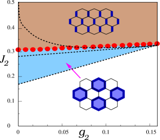
Figure 9: (Color online) Phase diagram of KMH model obtained by bond operator and plaquette operator methods.

V Conclusion

In summary, we explored the quantum phase diagram of the $S=1/2$ KMH model, using of exact diagonalizaion for a finite lattice and a bond operator and plaquette operator methods for infinite system size, with the focus on the regions of coupling space with high classically degeneracy. Here, we found that the Néel, PVBC and SD orderings found for $J_{1}-J_{2}$ Heisenberg model, adiabatically continues to the phase space of KMH model. The effect of spin-orbit term $g_{2}$, which reduces the $O_{3}$ symmetry of Heisenberg model to $O_{2}$ for KMH, is converting the isotropic Néel ordered (for $0<J_{2}\lesssim 0.2$) state to a planar Néel ordering in honeycomb plane. Moreover, the PVBC ordered state which is found to be the ground state of $J_{1}-J_{2}$ model, for $0.2\lesssim J_{2}/J_{1}\lesssim 0.35$, is adiabaticically continued into the classical phase III and lower part of phase IV. For $0.35\lesssim J_{2}/J_{1}\lesssim 0.5$, the SD ordering obtained for isotropic model extends toward upper part of phase IV and also into classically ordered phase II for $g_{2}<0.2$. Our work highlights the significance of quantum fluctuations for $S=1/2$ KMH model, in melting down the classically ordered state into purely quantum ground states.

Appendix A Self-consistent equation of bond operator mean field theory

The spin Hamiltonian 2 for an SD configuration can be rewritten as

$$\begin{split}H&=J_{1}{\sum}_{\langle ij\rangle\in{\rm bond}}{\bf S}_{i}.{\bf S}_{j}+(J_{2}-g_{2}){\sum}_{\langle ij\rangle\in{\rm bond}}{\bf S}_{i}.{\bf S}_{j}\\ &+2g_{2}{\sum}_{\langle ij\rangle\in{\rm bond}}{S}_{i}^{z}{S}_{j}^{z}+J_{1}{\sum}_{\langle ij\rangle\notin{\rm bond}}{\bf S}_{i}.{\bf S}_{j}\\ &+(J_{2}-g_{2}){\sum}_{\langle ij\rangle\notin{\rm bond}}{\bf S}_{i}.{\bf S}_{j}+2g_{2}{\sum}_{\langle ij\rangle\notin{\rm bond}}{S}_{i}^{z}{S}_{j}^{z}.\end{split}$$ (16)

Inserting the spin representations 10 into this Hamiltonian, assuming that all the singlets are condensed (this means replacing $s$ and $s^{\dagger}$ with the c-number $\bar{s}$), keeping only the quadratic terms, incorporating the constraint 11 by a Lagrange multiplier $\mu$, and finally the Fourier transformation, we obtain the following quadratic Hamiltonian in terms of the momentum space triplet operators

$${H^{[2]}}_{BO}=-N_{b}\frac{3}{4}J_{1}{\overline{s}}^{2}-N_{b}\mu{\overline{s}}^{2}+N_{b}\mu+$$

$${\sum}_{k>0}[(G_{k}+F_{k}^{1})({t^{\dagger}}_{k,{x}}{t_{k,{x}}}+{t^{\dagger}}_{-k,{x}}{t_{-k,{x}}})+$$

$$(G_{k}+F_{k}^{1})({t^{\dagger}}_{k,{y}}{t_{k,{y}}}+{t^{\dagger}}_{-k,{y}}{t_{-k,{y}}})+$$

$$(G_{k}+F_{k}^{2})({t^{\dagger}}_{k,{z}}{t_{k,{z}}}+{t^{\dagger}}_{-k,{z}}{t_{-k,{z}}})+$$

$$(F_{k}+F_{k}^{1})({t^{\dagger}}_{k,{x}}{{t^{\dagger}}_{-k,{x}}}+{t}_{k,{x}}{t_{-k,{x}}})+$$

$$(F_{k}+F_{k}^{1})({t^{\dagger}}_{k,{y}}{{t^{\dagger}}_{-k,{y}}}+{t}_{k,{y}}{t_{-k,{y}}})+$$

$$(F_{k}+F_{k}^{2})({t^{\dagger}}_{k,{z}}{{t^{\dagger}}_{-k,{z}}}+{t}_{k,{z}}{t_{-k,{z}}})],$$ (17)

where $N_{b}$ is the number of bonds and

$$G_{k}=\frac{J_{1}}{4}-\mu-\frac{{{\overline{s}}^{2}}}{4}J_{1}({\epsilon}_{k}+{\epsilon}_{-k})+\frac{{{\overline{s}}^{2}}}{4}J_{2}({\eta}_{k}+{\eta}_{-k})$$

$$F_{k}=-\frac{{{\overline{s}}^{2}}}{4}J_{1}({\epsilon}_{k}+{\epsilon}_{-k})+\frac{{{\overline{s}}^{2}}}{4}J_{2}({\eta}_{k}+{\eta}_{-k})$$

$$F_{k}^{1}=-\frac{{{\overline{s}}^{2}}}{4}g_{2}({\eta}_{k}+{\eta}_{-k})$$

$$F_{k}^{2}=\frac{{{\overline{s}}^{2}}}{4}g_{2}({\eta}_{k}+{\eta}_{-k}).$$ (18)

In the above relations ${\epsilon}_{k}$ and $\eta_{k}$ are defined as

$$\epsilon_{k} = e^{-ik_{b}}+e^{-i(k_{b}+k_{a})}$$

$$\eta_{k} = 2\left[\cos(k_{a})+\cos(k_{b})+\cos(k_{a}+k_{b})\right]$$ (19)

Using appropriate Bogoliubov transformations, the Hamiltonian 17 can be diagonalized as

$${H^{[2]}}_{BO}=N_{b}(-\frac{3}{4}J_{1}{\overline{s}}^{2}-\mu{\overline{s}}^{2}+\mu)+$$

$${\sum}_{k>0}({\omega}_{k,x}+{\omega}_{k,y}+{\omega}_{k,z}-3G_{k}-2F_{k}^{1}-F_{k}^{2})+$$

$${\sum}_{k>0}{\omega}_{k,x}({\gamma}_{k,x}^{{\dagger}}{{\gamma}}_{k,x}+{\gamma}_{-k,x}^{{\dagger}}{{\gamma}}_{-k,x})+$$

$${\sum}_{k>0}{\omega}_{k,y}({\gamma}_{k,y}^{{\dagger}}{{\gamma}}_{k,y}+{\gamma}_{-k,y}^{{\dagger}}{{\gamma}}_{-k,y})+$$

$${\sum}_{k>0}{\omega}_{k,z}({\gamma}_{k,z}^{{\dagger}}{{\gamma}}_{k,z}+{\gamma}_{-k,z}^{{\dagger}}{{\gamma}}_{-k,z}),$$ (20)

in which

$$\omega_{k,x}=\omega_{k,y}=\sqrt{({G_{k}}+F_{k}^{1})^{2}-({F_{k}}+F_{k}^{1})^{2}}$$

$$\omega_{k,z}=\sqrt{({G_{k}}+F_{k}^{2})^{2}-({F_{k}}+F_{k}^{2})^{2}},$$ (21)

are the triplon dispersions and

$${\epsilon}_{g}=(-\frac{3}{4}J_{1}{\overline{s}}^{2}-\mu{\overline{s}}^{2}+\mu)+$$

$${\sum}_{k>0}({\omega}_{k,x}+{\omega}_{k,y}+{\omega}_{k,z}-3G_{k}-2F_{k}^{1}-F_{k}^{2}),$$ (22)

gives the ground state energy per bond. The ground state energy depends on the parameters $\mu$ and ${\bar{s}}$, and can be determined self-consistently from the saddle-point conditions

$$\frac{\partial\epsilon_{g}}{\partial\mu} = -\overline{s}^{2}+1-2{\sum}_{k>0}\frac{(G_{k}+F_{k}^{1})}{\omega_{k,x}}$$

$$- {\sum}_{k>0}\frac{(G_{k}+F_{k}^{2})}{\omega_{k,z}}+3{\sum}_{k>0}1=0,$$

$$\frac{\partial\epsilon_{g}}{\partial{\overline{s}}^{2}} = -\frac{3}{4}J_{1}-\mu$$ (23)

$$+ 2{\sum}_{k>0}\left(-\frac{J_{1}}{4}({\epsilon}_{k}+{\epsilon}_{-k})+\right.\left.\frac{(J_{2}-g_{2})}{4}({\eta}_{k}+{\eta}_{-k})\right)$$

$$\times (\frac{G_{k}-F_{k}}{\omega_{k,x}}-1)$$

$$+ {\sum}_{k>0}\left(-\frac{J_{1}}{4}({\epsilon}_{k}+{\epsilon}_{-k})+\frac{(J_{2}-g_{2})}{4}({\eta}_{k}+{\eta}_{-k})\right)$$

$$\times (\frac{G_{k}-F_{k}}{\omega_{k,z}}-1)=0.$$

Appendix B Self consistent equations of plaquette mean field theory

Considering the PVBC ordering shown in Fig.4-b, the Hamiltonian 2 can be rewrited as

$$\begin{split}H&=J_{1}{\sum}_{\langle ij\rangle\in PL}{\bf S}_{i}.{\bf S}_{j}+(J_{2}-g_{2}){\sum}_{\langle ij\rangle\in PL}{\bf S}_{i}.{\bf S}_{j}\\ &+2g_{2}{\sum}_{\langle ij\rangle\in PL}{S}_{i}^{z}{S}_{j}^{z}+J_{1}{\sum}_{\langle ij\rangle\notin PL}{\bf S}_{i}.{\bf S}_{j}\\ &+(J_{2}-g_{2}){\sum}_{\langle ij\rangle\notin PL}{\bf S}_{i}.{\bf S}_{j}+2g_{2}{\sum}_{\langle ij\rangle\notin PL}{S}_{i}^{z}{S}_{j}^{z}.\end{split}$$ (24)

The Hamiltonian of a single hexagonal block can be represented in terms of creation and annihilation operators as

$$H_{PL}=\sum_{p}\epsilon_{s_{p}}s_{p}^{\dagger}s_{p}+\sum_{m}\epsilon_{t_{m}}{{t^{\dagger}}_{m\alpha}}{{t}_{m\alpha}},$$ (25)

where $\epsilon_{s}$ and $\epsilon_{t_{m}}$ are evaluated numerically by diagonalizing the KHM Hamiltonian in $S_{Z}=0$ basis in a hexagon. Reexpressing the Hamiltonian Eq.24 in these new singlet and triplet operators and, incorporating the constraint 15, using the Bogoliubov transformations, and assuming the condensation of singlets, we arrive at the following diagonalized Hamiltonian in ${\bf k}$-space,

$${H^{[2]}}_{PL}=N_{p}(\overline{s}^{2}\epsilon_{s_{1}}-\mu\overline{s}^{2}+\mu)+$$

$${\sum}_{k>0}({\omega}_{m,k}^{x}+{\omega}_{m,k}^{y}+{\omega}_{m,k}^{z}-3G_{m,k}-2G_{m,k}^{1}-G_{m,k}^{2})+$$

$${\sum}_{k>0}{\omega}_{m,k}^{x}({\gamma}_{m,kx}^{{\dagger}}{{\gamma}}_{m,kx}+{\gamma}_{m,-kx}^{{\dagger}}{{\gamma}}_{m,-kx})+$$

$${\sum}_{k>0}{\omega}_{m,k}^{y}({\gamma}_{m,ky}^{{\dagger}}{{\gamma}}_{m,ky}+{\gamma}_{m,-ky}^{{\dagger}}{{\gamma}}_{m,-ky})+$$

$${\sum}_{k>0}{\omega}_{m,k}^{z}({\gamma}_{m,kz}^{{\dagger}}{{\gamma}}_{m,kz}+{\gamma}_{m,-kz}^{{\dagger}}{{\gamma}}_{m,-kz}),$$ (26)

where

$$G_{m,k}=\epsilon_{t_{m}}-\mu+2J_{1}\overline{s}^{2}S_{m,k}^{1}+J_{2}S_{m,k}^{2}$$

$$F_{m,k}=2J_{1}\overline{s}^{2}S_{m,k}^{1}+J_{2}S_{m,k}^{2}$$

$$G_{m,k}^{1}=-g_{2}S_{m,k}^{2}=-G_{m,k}^{2}$$

$$S_{m,k}^{1}={a}_{2,m}{a}_{5,m}\cos(k_{a})+{a}_{3,m}{a}_{6,m}\cos(k_{b})+$$

$${a}_{1,m}{a}_{4,m}\cos(k_{a}+k_{b})$$

$$S_{m,k}^{2}=({a}_{5,m}{a}_{3,m}+{a}_{1,m}{a}_{5,m}+{a}_{2,m}{a}_{6,m}+{a}_{2,m}{a}_{4,m})$$

$$\times\cos(k_{a})+({a}_{1,m}{a}_{3,m}+{a}_{3,m}{a}_{5,m}+{a}_{4,m}{a}_{6,m}+{a}_{2,m}{a}_{6,m})$$

$$\times\cos(k_{b})+({a}_{1,m}{a}_{3,m}+{a}_{1,m}{a}_{5,m}+{a}_{4,m}{a}_{6,m}+{a}_{2,m}{a}_{4,m})$$

$$\times\cos(k_{a}+k_{b}),$$ (27)

in which

$$\omega_{m,k}^{x}=\omega_{m,k}^{y}=\sqrt{({G_{m,k}}+G_{m,k}^{1})^{2}-({F_{m,k}}+G_{m,k}^{1})^{2}}$$

$$\omega_{m,k}^{z}=\sqrt{({G_{m,k}}+G_{m,k}^{2})^{2}-({F_{m,k}}+G_{m,k}^{2})^{2}},$$ (28)

are the triplon dispersions and

$${\epsilon}_{g}=(J_{1}{\overline{s}}^{2}{\epsilon_{s_{1}}}-\mu{\overline{s}}^{2}+\mu)+$$

$${\sum}_{k>0}({\omega}_{m,k}^{x}+{\omega}_{m,k}^{y}+{\omega}_{m,k}^{z}-3G_{m,k}-2G_{m,k}^{1}-G_{m,k}^{2}),$$

is the ground state energy per plaquette. Minimization of B with respect to the chemical potential $\mu$ and condensate density ${\bar{s}}$, gives rise to the following self-consistent equations

$$\frac{\partial\epsilon_{g}}{\partial\mu} = -\overline{s}^{2}+1-2{\sum}_{k>0}\frac{(G_{m,kz}+G_{m,kz}^{2})}{\omega_{m,k}^{z}}$$

$$- 2{\sum}_{k>0}\frac{(G_{m,kx}+G_{m,kx}^{1})}{\omega_{m,k}^{x}}+3{\sum}_{k>0}1=0,$$

$$\frac{\partial\epsilon_{g}}{\partial{\overline{s}}^{2}} = {\epsilon_{s}}-\mu$$ (30)

$$+ {\sum}_{k>0}\left(({\epsilon_{t,m}^{z}-\mu})\frac{J_{1}S_{m,kz}^{1}+(J_{2}+g_{2})S_{m,kz}^{2}}{\omega_{m,k}^{z}}\right)$$

$$+ 2{\sum}_{k>0}\left(({\epsilon_{t,m}^{x}-\mu})\frac{J_{1}S_{m,kx}^{1}+(J_{2}-g_{2})S_{m,kx}^{2}}{\omega_{m,k}^{x}}\right)$$

$$- 2{\sum}_{k>0}\left(J_{1}S_{m,kx}^{1}+(J_{2}-g_{2})S_{m,kx}^{2}\right)$$

$$- {\sum}_{k>0}\left(J_{1}S_{m,kz}^{1}+(J_{2}+g_{2})S_{m,kz}^{2}\right)=0$$

whose solution provides us with the ground state energy of PVBC state.

References

- (1) L. Balent, Nature(London) 464, 199(2010).
- (2) J. B. Fouet, P. Sindzingre, and C. Lhuillier, Eur. Phys. J. B 20, 241 (2001).
- (3) S. Okumura, H. Kawamura, T. Okubo, and Y. Motome, J. Phys. Soc. Jpn. 79, 114705 (2010).
- (4) J. Villain, Z. Phys. B: Condens. Matter 33, 31 (1979).
- (5) F. Wang, Phys. Rev. B 82, 024419 (2010).
- (6) B. K. Clark, D. A. Abanin, and S. L. Sondhi, Phys. Rev. Lett. 107, 087204 (2011).
- (7) D. C. Cabra, C. A. Lamas, and H. D. Rosales Phys. Rev. B 83, 094506 (2011).
- (8) Y-M. Lu, and Y. Ran, Phys. Rev. B 84, 024420 (2011).
- (9) H. Zhang, and C. A. Lamas, Phys. Rev. B 87, 024415 (2013).
- (10) X-L. Yu, D-Y Liu, P. Li, and L-J. Zou, Physica E 59 41 (2014).
- (11) A. Mulder, R. Ganesh, L. Capriotti, and A. Paramekanti, 81, 214419 (2010).
- (12) H. Mosadeq, F. Shahbazi, and S. A. Jafari, J. Phys.: Condens. Matter, 23, 226006 (2011).
- (13) A. F. Albuquerque, D. Schwandt, B. Hetenyi, S. Capponi, M. Mambirini, and A. M. Lauchli, Phys. Rev. B 84, 024406 (2011).
- (14) J. Reuther, D. A. Abanin, and T. Thomale, Phys. Rev. B 84, 014417 (2011).
- (15) P. H. Y. Li, R. F. Bishop, D. J. J. Farnell, and C. E. Campbell, J. Phys.: Condens. Matter 24, 236002 (2012); Phys. Rev. B 86, 144404 (2012).
- (16) R. Ganesh, S. Nishimoto, and J. van den Brink, Phys. Rev. B 87, 054413 (2013).
- (17) Z. Zhu, D. A. Huse, and S. R. White, Phys. Rev. Lett. 110, 127205 (2013).
- (18) R. F. Bishop, P. H. Y. Li, and C. E. Campbell, J. Phys.: Condens. Matter 25 , 306002 (7pp) (2013).
- (19) C. L. Kane and E. J. Mele, Phys. Rev. Lett 95, 226801 (2005).
- (20) C. L. Kane and E. J. Mele, Phys. Rev. Lett. 95, 146802 (2005).
- (21) B. A. Bernevig and S.-C. Zhang, Phys. Rev. Lett. 96,106802 (2006).
- (22) B. A. Bernevig, T. L. Hughes, and S.-C. Zhang, Science 314, 1757 (2006).
- (23) M. König, S. Wiedmann, C. Brüne, A. Roth, H. Buhmann, L. W. Molenkamp, X.-L. Qi, and S.-C. Zhan, Science 318, 766 (2007).
- (24) M. Z. Hasan and C. L. Kane, Rev. Mod. Phys. 82, 3045 (2010).
- (25) X.-L. Qi and S.-C. Zhang, Rev. Mod. Phys. 83, 1057 (2011).
- (26) B. A. Bernevig, Topological Insulators and Topological Su-perconductors (Princeton University Press, Princeton and Oxford, 2013).
- (27) S. Rachel and K. Le Hur, Phys. Rev. B 82, 075106 (2010).
- (28) D. Soriano and J. Fernández-Rossier, Phys. Rev. B 82,161302 (2010).
- (29) Y. Yamaji and M. Imada, Phys. Rev. B 83, 205122 (2011).
- (30) D. Zheng, G.-M. Zhang, and C. Wu, Phys. Rev. B 84, 205121 (2011).
- (31) D.-H. Lee, Phys. Rev. Lett. 107, 166806 (2011).
- (32) S.-L. Yu, X. C. Xie, and J.-X. Li, Phys. Rev. Lett. 107, 010401 (2011).
- (33) M. Mardani, M.-S. Vaezi, and A. Vaezi, arXiv:1111.5980.
- (34) J. Wen, M. Kargarian, A. Vaezi, and G. A. Fiete, Phys. Rev. B 84, 235149 (2011).
- (35) M. Hohenadler, T. C. Lang, and F. F. Assaad, Phys. Rev. Lett. 106, 100403 (2011).
- (36) C. Griset and C. Xu, Phys. Rev. B 85, 045123 (2012).
- (37) W. Wu, S. Rachel, W.-M. Liu, and K. Le Hur, Phys. Rev. B 85, 205102 (2012).
- (38) M. Hohenadler, Z. Y. Meng, T. C. Lang, S. Wessel, A. Muramatsu, and F. F. Assaad, Phys. Rev. B 85, 115132 (2012).
- (39) S. Ueda, N. Kawakami, and M. Sigrist, Phys. Rev. B 87, 161108 (2013).
- (40) H.-H. Hung, L. Wang, Z.-C. Gu, and G. A. Fiete, Phys. Rev. B 87, 121113 (2013).
- (41) H.-H. Hung, V. Chua, L. Wang, and G. A. Fiete, Phys. Rev. B 89, 235104 (2014).
- (42) Z. Y. Meng, H.-H. Hung, and T. C. Lang, Mod. Phys. Lett B 28 143001 (2014).
- (43) Y. Araki, T. Kimura, A. Sekine, K. Nomura, and T. Z. Nakano, arXiv:1311.3973.
- (44) Y. Araki and T. Kimura, Phys. Rev. B 87, 205440 (2013).
- (45) F. F. Assaad, M. Bercx, and M. Hohenadler, Phys. Rev. X 3, 011015 (2013).
- (46) M. Laubach, J. Reuther, R. Thomale, and S. Rachel, arXiv:1312.2934.
- (47) M. H. Zare, F. Fazileh, and F. Shahbazi, Phys. Rev. B 87, 224416 (2013).
- (48) A.Vaezi, M.Mashkoori, and M. Hosseini, Phys. Rev. B 85, 195126 (2012).
- (49) S. M. Bhattacharjee, Z. Phys. B: Condensed Matter, 82 323 (1991).
- (50) M. Mambrini, A. Läuchli, D. Poilbanc, and F. Mila, Phys. Rev. B, 74, 144422 (2006)
- (51) A. V. Chubukov and Th. Jolicoeur, Phys. Rev. B 44, 12050 (1991).
- (52) S. Sachdev and R. N. Bhatt, Phys. Rev. B 41, 9323 (1990).