Heterogeneous Mean Field for neural networks with short term plasticity

Abstract

We report about the main dynamical features of a model of leaky-integrate-and fire excitatory neurons with short term plasticity defined on random massive networks. We investigate the dynamics by a Heterogeneous Mean–Field formulation of the model, that is able to reproduce dynamical phases characterized by the presence of quasi–synchronous events. This formulation allows one to solve also the inverse problem of reconstructing the in-degree distribution for different network topologies from the knowledge of the global activity field. We study the robustness of this inversion procedure, by providing numerical evidence that the in-degree distribution can be recovered also in the presence of noise and disorder in the external currents. Finally, we discuss the validity of the heterogeneous mean–field approach for sparse networks, with a sufficiently large average in–degree.

I Introduction

Physiological information about neural structure and activity was employed from the very beginning to construct effective mathematical models of brain functions. Typically, neural networks were introduced as assemblies of elementary dynamical units, that interact with each other through a graph of connections boccaletti . Under the stimulus of experimental investigations, these models have been including finer and finer details. For instance, the combination of complex single–neuron dynamics, delay and plasticity in synaptic evolution, endogenous noise and specific network topologies revealed quite crucial for reproducing experimental observations, like the spontaneous emergence of synchronized neural activity, both in vitro (see, e.g., volman ) and in vivo, and the appearance of peculiar fluctuations, the so–called “up–down” states, in cortical sensory areas miguel ; torres .

Since the brain activity is a dynamical process, its statistical description needs to take into account time as an intrinsic variable. Accordingly, non–equilibrium statistical mechanics should be the proper conceptual frame, where effective models of collective brain activity should be casted in. Moreover, the large number of units and the redundancy of connections suggest that a mean–field approach can be the right mathematical tool for understanding the large–scale dynamics of neural network models. Several analytical and numerical investigations have been devoted to mean field approaches to neural dynamics. In particular, stability analysis of asynchronous states in globally coupled networks and collective observables in highly connected sparse network can be deduced in relatively simple neural network models through mean field techniques mfbrunel ; mfcessac ; mfbress ; polmf ; millman .

In this paper we provide a detailed account of a mean–field approach, that has been inspired by the “heterogeneous mean–field” (HMF) formulation, recently introduced for general interacting networks vespignani ; mendes . The overall method is applied here to the simple case of random networks of leaky integrate–and–fire (LIF) excitatory neurons in the presence of synaptic plasticity. On the other hand, it can be applied to a much wider class of neural network models, based on a similar mathematical structure.

The main advantages of the HMF method are the following: (i) it can identify the relation between the dynamical properties of the global (synaptic) activity field and the network topology, (ii) it allows one to establish under which conditions partially synchronized or irregular firing events may appear , (iii) it provides a solution to the inverse problem of recovering the network structure from the features of the global activity field.

In Section II, we describe the network model of excitatory LIF neurons with short–term plasticity. The dynamical properties of the model are discussed at the beginning of Section III. In particular, we recall that the random structure of the network is responsible for the spontaneous organization of neurons in two families of locked and unlocked ones DLLPT . In the rest of this Section we summarize how to define a heterogeneous thermodynamic limit, that preserves the effects of the network randomness and allows one to transform the original dynamical model into its HMF representation BCDLV ). The HMF equations provide a relevant computational advantage with respect to the original system. Actually, they describe the dynamics of classes of equal–in–degree neurons, rather than that of individual neurons. In practice, one can take advantage of a suitable sampling, according to its probability distribution, of the continuous in–degree parameter present in the HMF formulation. For instance, by properly ”sampling” the HMF model into 300 equations one can obtain an effective description of the dynamics engendered by a random Erdös–Renyi network made of ${\mathcal{O}}(10^{4})$ neurons.

In Section IV we show that the HMF formulation allows also for a clear interpretation of the presence of classes of locked and unlocked neurons in QSE: they correspond to the presence of a fixed point or of an intermittent-like map of the return time of firing events, respectively. Moreover, we analyze in details the stability properties of the model and we find that any finite sampling of the HMF dynamics is chaotic, i.e. it is characterized by a positive maximum Lyapunov exponent, $\lambda_{\mathrm{m}ax}$. Its value depends indeed on the finite sampling of the in–degree parameter. On the other hand, chaos is found to be relatively weak and, when the number of samples, $M$, is increased, $\lambda_{\mathrm{m}ax}$ vanishes with a power–law decay, $M^{-\gamma}$, with $\gamma\sim 1/2$. This is consistent with the mean–field like nature of the HMF equations: in fact, it can be argued that, in the thermodynamic limit, any chaotic component of the dynamics should eventually disappear, as it happens for the original LIF model, when a naive thermodynamic limit is performed DLLPT .

In Section V we analyze the HMF dynamics for networks with different topologies (e.g., Erdös–Renyi and in particular scale free). We find that the dynamical phase characterized by QSE is robust with respect to the network topology and it can be observed only if the variance of the considered in–degree distributions is sufficiently small. In fact, quasi-synchronous events are suppressed for too broad in–degree distributions, thus yielding a transition between a fully asynchronous dynamical phase and a quasi-synchronous one, controlled by the variance of the in–degree distribution. In all the cases analyzed in this Section, we find that the global synaptic–activity field characterizes completely the dynamics in any network topology.

Accordingly, the HMF formulation appears as an effective algorithmic tool for solving the following inverse problem: given a global synaptic–activity field, which kind of network topology has generated it? In Section VI, after a summary of the numerical procedure used to solve such an inverse problem, we analyze the robustness of the method in two circumstances: $a)$ when a noise is added to the average synaptic–activity field, and $b)$ when there are noise and disorder in the external currents.

Such robustness studies are particularly relevant in view of applying this strategy to real data obtained from experiments. Finally, in Section VII we show that a HMF formulation can be straightforwardly extended to non–massive networks, i.e. random networks, where the in–degree does not increase proportionally to the number of neurons. In this case the relevant quantity in the HMF-like formulation is the average value of the in–degree distribution, and the HMF equations are expected to reproduce confidently the dynamics of non–massive networks, provided this average is sufficiently large. Conclusions and perspectives are contained in Section VIII.

II The model

We consider a network of $N$ excitatory LIF neurons interacting via a synaptic current and regulated by short–term plasticity, according to a model introduced in tsodyksnet . The membrane potential $V_{j}$ of each neuron evolves in time following the differential equation

$$\tau_{\mathrm{m}}\dot{V}_{j}=E_{\mathrm{c}}-V_{j}+R_{\mathrm{in}}I_{\mathrm{syn}}(j)\,,$$ (1)

where $\tau_{\mathrm{m}}$ is the membrane time constant, $R_{\mathrm{in}}$ is the membrane resistance, $I_{\mathrm{syn}}(j)$ is the synaptic current received by neuron $j$ from all its presynaptic neurons (see below for its mathematical definition) and $E_{\mathrm{c}}$ is the contribution of an external current (properly multiplied by a unit resistance).

Whenever the potential $V_{j}(t)$ reaches the threshold value $V_{\mathrm{th}}$, it is reset to $V_{\mathrm{r}}$, and a spike is sent towards the postsynaptic neurons. For the sake of simplicity the spike is assumed to be a $\delta$–like function of time. Accordingly, the spike–train $S_{j}(t)$ produced by neuron $j$, is defined as,

$$S_{j}(t)=\sum_{m}\delta(t-t_{j}(m)),$$ (2)

where $t_{j}(m)$ is the time when neuron $j$ fires its $m$-th spike.

The transmission of the spike–train $S_{j}(t)$ is mediated by the synaptic dynamics. We assume that all efferent synapses of a given neuron follow the same evolution (this is justified in so far as no inhibitory coupling is supposed to be present). The state of the $i$-th synapse is characterized by three variables, $x_{i}$, $y_{i}$, and $z_{i}$, which represent the fractions of synaptic transmitters in the recovered, active, and inactive state, respectively ($x_{i}+y_{i}+z_{i}=1$) plast1 ; plast2 ; tsodyksnet . The evolution equations are

$$\dot{y}_{i}=-\frac{y_{i}}{\tau_{\mathrm{in}}}+ux_{i}S_{i}$$ (3)

$$\dot{z}_{i}=\frac{y_{i}}{\tau_{\mathrm{in}}}-\frac{z_{i}}{\tau_{\mathrm{r}}}\ .$$ (4)

Only the active transmitters react to the incoming spikes: the parameter $u$ tunes their effectiveness. Moreover, $\tau_{\mathrm{in}}$ is the characteristic decay time of the postsynaptic current, while $\tau_{\mathrm{r}}$ is the recovery time from synaptic depression. For the sake of simplicity, we assume also that all parameters appearing in the above equations are independent of the neuron indices. The model equations are finally closed, by representing the synaptic current as the sum of all the active transmitters delivered to neuron $j$

$$I_{\mathrm{syn}}(j)=\frac{G}{N}\sum_{i\neq j}\epsilon_{ij}y_{i},$$ (5)

where $G$ is the strength of the synaptic coupling (that we assume independent of both $i$ and $j$), while $\epsilon_{ij}$ is the directed connectivity matrix whose entries are set equal to 1 or 0 if the presynaptic neuron $i$ is connected or disconnected with the postsynaptic neuron $j$, respectively. Since we suppose the input resistance $R_{\mathrm{in}}$ independent of $j$, it can be included into $G$. In this paper we study the case of excitatory coupling between neurons, i.e. $G>0$. We assume that each neuron is connected to a macroscopic number, ${\mathcal{O}}(N)$, of pre-synaptic neurons: this is the reason why the sum is divided by the factor $N$. Typical values of the parameters contained in the model have phenomenological origin volman ; tsodyksnet . Unless otherwise stated, we adopt the following set of values: $\tau_{\mathrm{in}}=6$ ms, $\tau_{\mathrm{m}}=30$ ms, $\tau_{\mathrm{r}}=798$ ms, $V_{\mathrm{r}}=13.5$ mV, $V_{\mathrm{th}}=15$ mV, $E_{\mathrm{c}}=15.45$ mV, ${G}=45$ mV and $u=0.5$. Numerical simulations can be performed much more effectively by introducing dimensionless quantities,

$$a=\frac{E_{c}-V_{\mathrm{r}}}{V_{\mathrm{th}}-V_{\mathrm{r}}}$$ (6)

$$g=\frac{G}{V_{\mathrm{th}}-V_{\mathrm{r}}}$$ (7)

$$v=\frac{V-V_{\mathrm{r}}}{V_{\mathrm{th}}-V_{\mathrm{r}}},$$ (8)

and by rescaling time, together with all the other temporal parameters, in units of the membrane time constant $\tau_{\mathrm{m}}$ (for simplicity, we leave the notation unchanged after rescaling). The values of the rescaled parameters are: $\tau_{\mathrm{in}}=0.2$, $\tau_{\mathrm{r}}=133\tau_{\mathrm{in}}$, $v_{\mathrm{r}}=0$, $v_{\mathrm{th}}=1$, $a=1.3$, $g=30$ and $u=0.5$. As to the normalized external current $a$, its value for the first part of our analysis corresponds to the firing regime for neurons. While the rescaled Eqs. (3) and (4) keep the same form, Eq. (1) changes to,

$$\dot{v}_{j}=a-v_{j}+\frac{g}{N}\sum_{i\neq j}\epsilon_{ij}y_{i}\,.$$ (9)

A major advantage for numerical simulations comes from the possibility of transforming the set of differential equations (3)–(5) and (9) into an event–driven map (for details see DLLPT and also brette ; zill ).

III Dynamics and heterogeneous mean field limit

The dynamics of the fully coupled neural network (i.e., $\epsilon_{ij}=1,\,\forall i,j$), described by Eq.s (9) and (2)–(5), converges to a periodic synchronous state, where all neurons fire simultaneously and the period depends on the model parameters DLLPT . A more interesting dynamical regime appears when some disorder is introduced in the network structure. For instance, this can be obtained by maintaining each link between neurons with probability $p$, so that the in-degree of a neuron (i.e. the number of presynaptic connections acting on it) takes the average value $\langle k_{i}\rangle=pN$, and the standard deviation of the corresponding in-degree distribution is given by the relation $\sigma_{k}=\sqrt{Np(1-p)}$. In such an Erdös-Renyi random network one typically observes quasi–synchronous events (QSE), where a large fraction of neurons fire in a short time interval of a few milliseconds, separated by an irregular firing activity lasting over some tens of ms (e.g., see DLLPT ). This dynamical regime emerges as a collective phenomenon, where neurons separate spontaneously into two different families: the locked and the unlocked ones. Locked neurons determine the QSE and exhibit a periodic behavior, with a common period but different phases. Their in–degree $k_{i}$ ranges over a finite interval below the average value $\langle k_{i}\rangle$. The unlocked ones participate to the irregular firing activity and exhibit a sort of intermittent evolution DLLPT . Their in-degree is either very small or higher than $\langle k_{i}\rangle$.

As the dynamics is very sensitive to the different values of of $k_{i}$, in a recent publication BCDLV we have shown that one can design a heterogeneous mean-field (HMF) approach by a suitable thermodynamic limit preserving, for increasing values of $N$, the main features associated with topological disorder. The basic step of this approach is the introduction of a probability distribution, $P(\tilde{k})$, for the normalized in-degree variable ${\tilde{k}}=k/N$, where the average $\langle\tilde{k}\rangle$ and the variance $\sigma_{\tilde{k}}^{2}=\langle{\tilde{k}}^{2}\rangle-\langle\tilde{k}\rangle^{2}$ are fixed independently of $N$. A realization of the random network containing $N$ nodes (neurons) is obtained by extracting for each neuron $i$ ($i=1,\cdots,N$) a value $\tilde{k}_{i}$ from $P(\tilde{k})$, and by connecting the neuron $i$ with $\tilde{k}_{i}N$ randomly chosen neurons (i.e., $\epsilon_{i,j}=1$, $j(i)=1,\cdots,\tilde{k}_{i}N$). For instance, one can consider a suitably normalized Gaussian–like distribution defined on the compact support, $\tilde{k}\in(0,1]$, centered around $\langle\tilde{k}\rangle$ with a sufficiently small value of the standard deviation $\sigma_{\tilde{k}}$, so that the tails of the distribution vanish at the boundaries of the support.

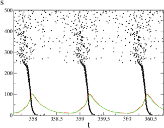
Figure 1: Raster plot of a randomly diluted network containing 500 neurons, ordered along the vertical axis according to their in–degree. The distribution $P(\tilde{k})$ is a Gaussian with $\langle\tilde{k}\rangle=0.7$, standard deviation $\sigma_{\tilde{k}}=0.077$. A black dot in the raster plot indicates that neuron $s$ has fired at time $t$. The red line is the global field $Y(t)$ and the green curve is its analytic fit by the function $Y_{f}(t)=Ae^{-\frac{t}{\tau_{1}}}+B(e^{\frac{t}{\tau_{2}}}-1)$, that repeats over each period of $Y(t)$; the parameter values are $A=2\cdot 10^{-2}$, $B=3.56\cdot 10^{-6}$, $\tau_{1}=0.268$ and $\tau_{2}=0.141$. Notice that the amplitude of both $Y(t)$ and $Y_{f}(t)$ has been suitably rescaled to be appreciated on the same scale of the Raster plot.

In Fig.1 we show the raster plot for a network of $N=500$ neurons and a Gaussian distribution $P(\tilde{k})$ with $\langle\tilde{k}\rangle=0.7$ and $\sigma_{\tilde{k}}=0.077$. One can observe a quasi-synchronous dynamics characterized by the presence of locked and unlocked neurons, and such a distinctive dynamical feature is preserved in the thermodynamic limit BCDLV . For example the time average of the inter–spike time interval between firing events of each neuron, (in formulae $ISI_{m}=t_{m}-t_{m-1}$, where the integer $m$ labels the $m$-th firing event) as a function of the connectivity $\tilde{k}$ is, apart from fluctuations, the same for each network size $N$. This confirms that the main features of the dynamics are maintained for increasing values of $N$.

The main advantage of this approach is that one can explicitly perform the limit $N\to\infty$ on the set of equations (9) and (2)–(5), thus obtaining the corresponding HMF equations:

$$\dot{v}_{\tilde{k}}(t)=a-v_{\tilde{k}}(t)+g\tilde{k}Y(t)$$ (10)

$$S_{\tilde{k}}(t)=\sum_{m}\delta(t-t_{\tilde{k}}(m))$$ (11)

$$\dot{y}_{\tilde{k}}(t)=-\frac{y_{\tilde{k}}(t)}{\tau_{\mathrm{in}}}+u(1-y_{\tilde{k}}(t)-z_{\tilde{k}}(t))S_{\tilde{k}}(t)$$ (12)

$$\dot{z}_{\tilde{k}}(t)=\frac{y_{\tilde{k}}(t)}{\tau_{\mathrm{in}}}-\frac{z_{\tilde{k}}(t)}{\tau_{\mathrm{r}}}$$ (13)

$$Y(t)=\int_{0}^{1}P(\tilde{k})y_{\tilde{k}}(t)d\tilde{k}.$$ (14)

The dynamical variables depend now on the continuous in–degree index $\tilde{k}$, and this set of equations represents the dynamics of equivalence classes of neurons. In fact, in this HMF formulation, neurons with the same $\tilde{k}$ follow the same evolution vespignani ; mendes . In practice, Eq.s (10)–(14) can be integrated numerically by sampling the probability distribution $P(\tilde{k})$: one can subdivide the support $(0,1]$ of $\tilde{k}$ by $M$ values $\tilde{k}_{i}\,\,\,(i=1,\cdots,M)$, in such a way that $\int_{\tilde{k}_{i}}^{\tilde{k}_{i+1}}P(\tilde{k})d\tilde{k}$ is constant (importance sampling). Notice that the integration of the discretized HMF equations is much less time consuming than the simulations performed on a random network. For instance, numerical tests indicate that the dynamics of a network with $N=10^{4}$ neurons can be confidently reproduced by an importance sampling with $M=300$.

The effect of the discretization of ${\tilde{k}}$ on the HMF dynamics can be analyzed by considering the distance $d(Y_{M_{1}}(t),Y_{M_{2}}(t))$ between the global activity fields $Y_{M_{1}}(t)$ and $Y_{M_{2}}(t)$ (see Eq.(14)) obtained for two different values $M_{1}$ and $M_{2}$ of the sampling, i.e.:

$$d(Y_{M_{1}}(t),Y_{M_{2}}(t))=\Bigg{(}\frac{1}{T}\sum_{i=1}^{T}\frac{(Y_{M_{1}}(t_{i})-Y_{M_{2}}(t_{i}))^{2}}{Y_{M_{1}}(t_{i})^{2}}\Bigg{)}^{\frac{1}{2}}.$$ (15)

In general $Y(t)$ exhibits a quasi periodic behavior and $d(Y_{M_{1}}(t),Y_{M_{2}}(t))$ is evaluated over a time interval equal to its period $T$. In order to avoid an overestimation of $d(Y_{M_{1}}(t),Y_{M_{2}}(t))$ due to different initial conditions, the field $Y_{2}(t)$ is suitably translated in time in order to make its first maximum coincide with the first maximum of $Y_{1}(t)$ in the time interval $[1,T]$. In Fig. 2 we plot $d_{M}=d(Y_{M},Y_{M/2})$ as a function of $M$. We find that $d_{M}\sim 1/\sqrt{M}$, thus confirming that the finite size simulation of the HMF dynamics is consistent with the HMF model ($M\to\infty$).

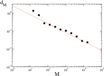
Figure 2: (Color online) The effect of sampling the probability distribution $P(\tilde{k})$ with $M$ classes of neurons in the HMF dynamics. Finite size effects are controlled by plotting the distance between the activity fields obtained for two sampling values $M$ and $M/2$, $d_{M}=d(Y_{M}(t),Y_{M/2}(t))$ (defined in the text), vs. $M$. The red dashed line is the power law $1/\sqrt{M}$. Data is obtained for a Gaussian distribution $P(\tilde{k})$, with $\langle\tilde{k}\rangle=0.7$ and $\sigma_{\tilde{k}}=0.077$.

As a final remark, notice that the presence of short–term synaptic plasticity plays a fundamental role in determining the partially synchronized regime. In fact, numerical simulations show that the discretized HMF dynamics without plasticity, i.e. $Y(t)=\int_{0}^{1}P(\tilde{k})S_{\tilde{k}}(t)d\tilde{k}$, converges to a synchronous periodic dynamics for any value of $M$ DL .

IV Stability analysis of the HMF dynamics

In the HMF equations (10)–(14) the dynamics of each neuron is determined by its in–degree $\tilde{k}$ and by the global synaptic activity field $Y(t)$. For the stability analysis of these equations, we follow a procedure introduced in tso_locked and employed also in BCDLV . For sufficiently large $M$ the discretized HMF dynamics allows one to obtain a precise fit of the periodic function $Y(t)$ and to estimate its period $T$. As an instance of its periodic behavior, in Fig.1 we report also $Y(t)$ (red line) and its fit (green line and the formula in the caption). The fitted field is exactly periodic and is a good approximation of the global field that one expects to observe in the mean field model corresponding to an infinite discretization $M$. As a result, the analysis performed using this periodic field are relative to the dynamics of the HMF model, i.e. in the limit $M\to\infty$. Using this fit, one can represent the dynamics of each class $\tilde{k}$ of neurons by the discrete–time map

$$\tau_{\tilde{k}}(n+1)=R_{\tilde{k}}[\tau_{\tilde{k}}(n)],$$ (16)

where $\tau_{\tilde{k}}(n)=|t_{\tilde{k}}(n)-nT|$ is the modulus of the time difference between the $n$-th spike of neuron $\tilde{k}$ and $nT$, i.e. the $n$-th QSE, that is conventionally identified by the corresponding maximum of $Y(t)$ (see Fig. 1).

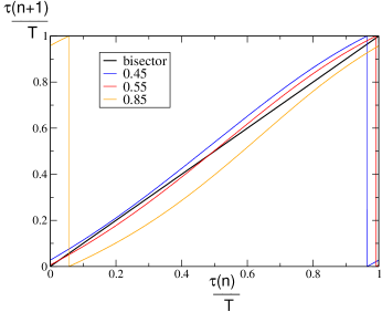
Figure 3: The return map $R_{\tilde{k}}$ of the rescaled variable $\tau_{\tilde{k}}/T$ (see Eq.(16)) for different values of $\tilde{k}$, corresponding to lines of different colors (see the legend in the inset: the black line is the bisector of the square).

In Fig. 3 we show $R_{\tilde{k}}$ for different values of $\tilde{k}$. The map of each class of locked neurons has a stable fixed point, whose value decreases with $\tilde{k}$. As a consequence, different classes of locked neurons share the same periodic behavior, but exhibit different phase shifts with respect to the maximum of $Y(t)$. This analysis describes in a clear mathematical language what is observed in simulations (see Fig 1): equally periodic classes of locked neurons determine the QSE by firing sequentially, over a very short time interval, that depends on their relative phase shift. In general, the values of $\tilde{k}$ identifying the family of locked neurons belong to a subinterval $(\tilde{k}_{1},\tilde{k}_{2})$ of $(0,1]$: the values of $\tilde{k}_{1}$ and $\tilde{k}_{2}$ mainly depend on $P(\tilde{k})$ and on its standard deviation $\sigma_{\tilde{k}}$ (more details are reported in BCDLV ). For what concerns unlocked neurons, $R_{\tilde{k}}$ exhibits the features of an intermittent-like dynamics. In fact, unlocked neurons with $\tilde{k}$ close to $\tilde{k}_{1}$ and $\tilde{k}_{2}$ spend a long time in an almost periodic firing activity, contributing to a QSE, then they depart from it, firing irregularly before possibly coming back again close to a QSE. The duration of the irregular firing activity of unlocked neurons typically increases for values of $\tilde{k}$ far from the interval $(\tilde{k}_{1},\tilde{k}_{2})$.

Using the deterministic map (16), one can tackle in full rigor the stability problem of the HMF model. The existence of stable fixed points for the locked neurons implies that they yield a negative Lyapunov exponent associated with their periodic evolution.

As for the unlocked neurons, their Lyapunov exponent, $\lambda_{\tilde{k}}$, can be calculated numerically by the time-averaged expansion rate of nearby orbits of map (16):

$$\lambda_{\tilde{k}}(n)=\frac{1}{n}\sum_{j=1}^{n}\mathrm{log}\Bigg{[}\frac{|\delta(j)|}{|\delta(0)|}\Bigg{]},$$ (17)

where $\delta(0)$ is the initial distance between nearby orbits and $\delta(j)$ is their distance at the $j$–th iterate, so that

$$\lambda_{\tilde{k}}=\lim_{n\to\infty}\lambda_{\tilde{k}}(n)$$ (18)

if this limit exists. The Lyapunov exponents for the unlocked component vanish as $\lambda_{\tilde{k}}(n)\sim 1/n$. According to these results, one expects that the maximum Lyapunov exponent $\lambda_{\mathrm{max}}(M)$ goes to zero in the limit $M\to\infty$. In fact, at each finite $M$, $\lambda_{\mathrm{max}}$ can be evaluated by using the standard algorithm by Benettin et al. BGGS . In Fig.4 we plot $\lambda_{\mathrm{max}}$ as a function of the discretization parameter $M$. Thus, $\lambda_{\mathrm{max}}(M)$ is positive, behaving approximately as $M^{-\gamma}$, with $\gamma\sim 1/2$ (actually, we find $\gamma=0.55$).

The scenario in any discretized version of the HMF dynamics is the following: (i) all unlocked neurons exhibit positive Lyapunov exponents, i.e. they represent the chaotic component of the dynamics; (ii) $\lambda_{\mathrm{max}}$ is typically quite small, and its value depends on the discretization parameter $M$ and on $P(\tilde{k})$; (iii) in the limit $M\to\infty$ $\lambda_{\mathrm{max}}$ and all $\lambda_{\tilde{k}}$’s of unlocked neurons vanish, thus converging to a quasi periodic dynamics, while the locked neurons persist in their periodic behavior.

The same scenario is observed in the dynamics of random networks built with the HMF strategy, where the variance of the distribution $P(\tilde{k})$ is kept independent of the system size $N$, so that the fraction of locked neurons is constant.

For the LIF dynamics in an Eördos–Renyi random network with $N$ neurons, it was found that $\lambda_{\mathrm{max}}(N)\approx N^{-0.27}$ in the limit $N\to\infty$ DLLPT . According to the argument proposed in DLLPT , the value of the power-law exponent is associated to the scaling of the number of unlocked neurons, $N_{u}$ with the system size $N$, namely $N_{u}\sim N^{0.9}$. The same argument applied to HMF dynamics indicates that the exponent $\gamma\sim 1/2$, ruling the vanishing of $\lambda_{\mathrm{max}}(M)$ in the limit $M\to\infty$, stems from the fact that the HMF dynamics keeps the fraction of unlocked neurons constant.

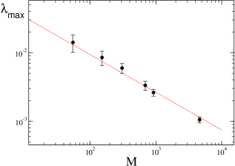
Figure 4: (Color online) The maximum Lyapunov exponent $\lambda_{\mathrm{max}}$ as a function of the sampling parameter $M$: $\lambda_{\mathrm{max}}$ has been averaged also over ten different realizations of the network (the error bars refer to the maximum deviation from the average). The dashed red line is the powerlaw $M^{-\gamma}$, with $\gamma=0.55$.

When the distribution $P(\tilde{k})$ is sufficiently broad, the system becomes asynchronous and locked neurons disappear. The global field $Y(t)$ exhibits fluctuations due to finite size effects and in the thermodynamic limit it tends to a constant value $Y^{*}$. From Eq.s (10)–(13), one obtains that in this regime each neuron with in–degree $\tilde{k}$ fires periodically with a period

$$T_{\tilde{k}}=\mathrm{ln}\Bigg{[}\frac{b+g\tilde{k}Y^{*}}{b+g\tilde{k}Y^{*}-1}\Bigg{]}~{},$$

while its phase depends on the initial conditions. In this case all the Lyapunov exponents $\lambda_{\tilde{k}}$ are negative.

V Topology and collective behavior

For a given in–degree probability distribution $P(\tilde{k})$, the fraction of locked neurons (i.e., $f_{\mathrm{l}}=\int_{\tilde{k}_{1}}^{\tilde{k}_{2}}P(\tilde{k})d\tilde{k}$) decreases by increasing $\sigma_{\tilde{k}}$ BCDLV . In particular, there is a critical value $\sigma^{*}$ at which $f_{\mathrm{l}}$ vanishes. This signals a very interesting dynamical transition between the quasi-synchronous phase ($\sigma_{\tilde{k}}<\sigma^{*}$) to a multi-periodic phase ($\sigma_{\tilde{k}}>\sigma^{*}$), where all neurons are periodic with different periods. Here we focus on the different collective dynamics that may emerge for choices of $P(\tilde{k})$ other than the Gaussian case, discussed in the previous section.

First, we consider a power–law distribution

$$P(\tilde{k})=A\tilde{k}^{-\alpha},$$ (19)

where the constant $A$ is given by the normalization condition $\int_{\tilde{k}_{m}}^{1}P(\tilde{k})d\tilde{k}=1$. The lower bound $\tilde{k}_{m}$ is introduced in order to maintain $A$ finite. For simplicity, we fix the parameter $\tilde{k}_{m}$ and analyze the dynamics by varying $\alpha$. Notice that the standard deviation $\sigma_{\tilde{k}}$ of distribution (19) decreases for increasing values of $\alpha$. The dynamics for relatively high $\alpha$ is very similar to the quasi–synchronous regime observed for $\sigma_{\tilde{k}}<\sigma^{*}$ in the Gaussian case (see Fig. 1). By decreasing $\alpha$ one can observe again a transition to the asynchronous phase observed for $\sigma_{\tilde{k}}>\sigma^{*}$ in the Gaussian case. Accordingly, also for the power–law distribution (19) a phase with locked neurons may set in only when there is a sufficiently large group of neurons sharing close values of $\tilde{k}$. In fact, the group of locked neurons is concentrated at values of $\tilde{k}$ quite close to the lower bound $\tilde{k}_{m}$, while in the Gaussian case they concentrate at values smaller than $\langle\tilde{k}\rangle$.

Another distribution, generating an interesting dynamical phase, is

$$P(\tilde{k})=B\mathrm{exp}\Bigg{(}-\frac{(\tilde{k}-p_{1})^{2}}{2\sigma_{s}^{2}}\Bigg{)}+B\mathrm{exp}\Bigg{(}-\frac{(\tilde{k}-p_{2})^{2}}{2\sigma_{s}^{2}}\Bigg{)},$$ (20)

i.e. the sum of two Gaussians peaked around different values, $p_{1}$ and $p_{2}$, of $\tilde{k}$, with the same variance $\sigma_{s}^{2}$. $B$ is the normalization constant such that $\int_{0}^{1}P(\tilde{k})=1$. We fix $p_{1}=0.5$ and vary both the variance, $\sigma_{s}$, and the distance between the peaks, $\Delta=|p_{2}-p_{1}|$.

If $\sigma_{s}$ is very large ($\sigma\gtrsim 0.1$), the situation is the same observed for a single Gaussian with large variance, yielding a multi–periodic asynchronous dynamical phase.

For intermediate values of $\sigma_{s}$ i.e. $0.05\lesssim\sigma\lesssim 0.1$, the dynamics of the network can exhibit a quasi–synchronous phase or a multi–periodic asynchronous phase, depending on the value of $\Delta$. In fact, one can easily realize that this parameter tunes the standard deviation of the overall distribution: small separations amount to broad distributions.

Finally, when $\sigma_{s}\lesssim 0.05$, a new dynamical phase appears.

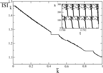
Figure 5: The time average of the inter–spike interval $\overline{ISI_{\tilde{k}}}$ vs. $\tilde{k}$ for the probability distribution $P(\tilde{k})$ defined in Eq.(20), with $\Delta=|p_{2}-p_{1}|=0.4$, and $\sigma_{\mathrm{s}}=0.03$. We have obtained the global field $Y(t)$ simulating the HMF dynamics with a discretization with $M=300$ classes of neurons. We have then used $Y(t)$ to calculate the $ISI$ of neurons evolving Eq. (10). In the inset we show the raster plot of the dynamics: as in Fig.1, neurons are ordered along the vertical axis according to their in–degree.

For small values of $\Delta$ (e.g. $\Delta\approx 0.1$) , we observe the usual QSE scenario with one family of locked neurons (data not shown). However, when $\Delta$ is sufficiently large (e.g. $\Delta\approx 0.4$), each peak of the distribution generates its own group of locked neurons. More precisely, neurons separate into three different sets: two locked groups, that evolve with different periods, $T_{1}$ and $T_{2}$, and the unlocked group. In Fig.5 we show the dependence of $\overline{ISI_{\tilde{k}}}$ on $\tilde{k}$ and the raster plot of the dynamics (see the inset) for $\sigma_{s}=0.03$ . Notice that the plateaus of locked neurons extend over values of $\tilde{k}$ on the left of $p_{1}$ and $p_{2}$. In the inset of Fig. 6 we plot the global activity field $Y(t)$: the peaks signal the quasi-synchronous firing events of the two groups of locked neurons. One can also observe that very long oscillations are present over a time scale much larger than $T_{1}$ and $T_{2}$. They are the effect of the firing synchrony of the of two locked families. In fact, the two frequencies $\omega_{1}=2\pi/T_{1}$ and $\omega_{2}=2\pi/T_{2}$ are in general not commensurate, and the resulting global field is a quasi–periodic function. This can be better appreciated by looking at Fig.6, where we report the frequency spectrum of the signal $Y(t)$ (red curve). We observe peaks at frequencies $\omega=n\omega_{1}+m\omega_{2}$, for integer values of $n$ and $m$. For comparison, we report also the spectrum of a periodic $Y(t)$, generated by the HMF with power law probability distribution (19), with $\alpha=4.9$ (black curve): in this case the peaks are located at frequencies multiples of the frequency of the locked group of neurons.

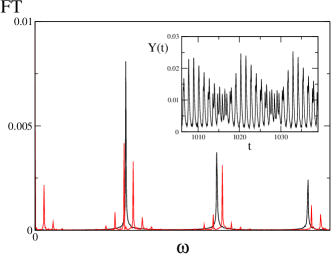
Figure 6: The frequency spectra of the global activity field $Y(t)$ for different in–degree probability distributions. The black spectrum has been obtained for the HMF dynamics with $M=350$, generated by the power law probability distribution $P(\tilde{k})\sim\tilde{k}^{-4.9}$ (see Eq.(19)), with $\tilde{k}_{m}=0.1$: in this case there is a unique family of locked neurons generating a periodic global activity field $Y(t)$. The red spectrum has been obtained for a random network of $N=300$ neurons generated by the double Gaussian distribution (see Eq.(20)) described in Fig.s 6 and 7: in this case two families of locked neurons are present while, as reported in the inset, $Y(t)$ exhibits a quasi–periodic evolution.

On the basis of this analysis, we can conclude that slow oscillations of the global activity field $Y(t)$ may signal the presence of more than one group of topologically homogeneous (i.e. locked) neurons. Moreover, we have also learnt that one can generate a large variety of global synaptic activity fields by selecting suitable in-degree distributions $P(\tilde{k})$, thus unveiling unexpected perspectives for exploiting a sort of topological engineering of the neural signals. For instance, one could investigate which kind of $P(\tilde{k})$ could give rise to an almost resonant dynamics, where $\omega_{2}$ is close to a multiple of $\omega_{1}$.

VI HMF and the Inverse problem in presence of noise

The HMF formulation allows one to define and solve the following global inverse problem: how to recover the in–degree distribution $P(\tilde{k})$ from the knowledge of the global synaptic activity field $Y(t)$ BCDLV .

Here we just sketch the basic steps of the procedure. Given $Y(t)$, each class of neurons of in-degree $\tilde{k}$ evolves according to the HMF equations:

$$\dot{\mathcal{V}}_{\tilde{k}}(t)=a-\mathcal{V}_{\tilde{k}}(t)+g\tilde{k}Y(t)$$ (21)

$$\dot{\mathcal{Y}}_{\tilde{k}}(t)=-\frac{\mathcal{Y}_{\tilde{k}}(t)}{\tau_{\mathsf{in}}}+u(1-\mathcal{Y}_{\tilde{k}}(t)-\mathcal{Z}_{\tilde{k}}(t))\tilde{S}_{\tilde{k}}(t)$$ (22)

$$\dot{\mathcal{Z}}_{\tilde{k}}(t)=\frac{\mathcal{Y}_{\tilde{k}}(t)}{\tau_{\mathsf{in}}}-\frac{\mathcal{Z}_{\tilde{k}}(t)}{\tau_{\mathsf{r}}}\,\,\,.$$ (23)

The different fonts used here, with respect to Eq.s (10)–(14), point out that in this framework the choice of the initial conditions is arbitrary and the dynamical variables $\mathcal{V}(t)$, $\mathcal{Y}(t)$, $\mathcal{Z}(t)$ in general may take different values from those assumed by $v(t)$, $y(t)$, $z(t)$, i.e. the variables generating $Y(t)$ in (10)–(14). However, one can exploit the self consistent relation for the global field $Y(t)$:

$$Y(t)=\int_{0}^{1}P({\tilde{k}})\mathcal{Y}_{\tilde{k}}(t)d{\tilde{k}}\,\,\,.$$ (24)

If $Y(t)$ and $\mathcal{Y}_{\tilde{k}}(t)$ are known, this is a Fredholm equation of the first kind for the unknown $P(\tilde{k})$ kress . If $Y(t)$ is a periodic signal, Eq. (24) can be easily solved by a functional Montecarlo minimization procedure, yielding a faithful reconstruction of $P(\tilde{k})$ BCDLV . This method applies successfully also when $Y(t)$ is a quasi-periodic signal, like the one generated by in–degree distribution (20).

In this section we want to study the robustness of the HMF equations and of the corresponding inverse problem procedure in the presence of noise. This is quite an important test for the reliability of the overall HMF approach. In fact, a real neural structure is always affected by some level of noise, that, for instance, may emerge in the form of fluctuations of ionic or synaptic currents. Moreover, it has been observed that noise is crucial for reproducing dynamical phases, that exhibit some peculiar synchronization patterns observed in in vitro experiments volman ; DL .

For the sake of simplicity, here we introduce noise by turning the external current $a$, in Eq. (10), from a constant to a time and neuron dependent stochastic processes $a_{\tilde{k}}(t)$. Precisely, the $a_{\tilde{k}}(t)$ are assumed to be i.i.d. stochastic variables, that evolve in time as a random walk with boundaries, $a_{\mathrm{min}}$ and $a_{\mathrm{max}}$ (the same rule adopted in DL ). Accordingly, the average value, $\bar{a}$ of $a_{\tilde{k}}(t)$ is given by the expression $\bar{a}=(a_{\mathrm{min}}+a_{\mathrm{max}})/2$, while the amplitude of fluctuations is $\delta=a_{\mathrm{max}}-a_{\mathrm{min}}$. At each step of the walk, the values of $a_{\tilde{k}}(t)$ are independently updated by adding or subtracting, with equal probability, a fixed increment $\Delta a$. Whenever the value of $a_{\tilde{k}}(t)$ crosses one of the boundaries, it is reset to the boundary value.

Since the dynamics has lost its deterministic character, its numerical integration cannot exploit an event driven algorithm, and one has to integrate Eq.s (10) –(13) by a scheme based on explicit time discretization. The results reported hereafter refer to an integration time step $\Delta t=9\cdot 10^{-4}$, that guarantees an effective sampling of the dynamics over the whole range of parameter values that we have explored. We have assumed that $\Delta t$ is also the time step of the stochastic evolution of $a_{\tilde{k}}(t)$.

Here we consider the case of uncorrelated noise, that can be obtained by a suitable choice of $\Delta a$ DL . In our simulations $\Delta a=10^{-2}$, that yields a value $\mathcal{O}(10^{-2})$ of the correlation time of the random walk with boundaries. This value, much smaller than the value $\mathcal{O}(1)$ typical of the ISI of neurons, makes the stochastic evolution of the external currents, $a_{\tilde{k}}(t)$, an effectively uncorrelated process with respect to the typical time scales of the neural dynamics.

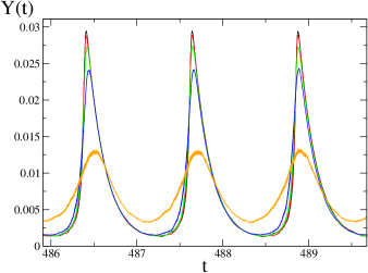
Figure 7: The global activity field $Y(t)$ of the HMF dynamics, sampled by $M=4525$ classes of neurons, for a gaussian probability distribution $P(\tilde{k})$, with $\langle\tilde{k}\rangle=0.7$ and $\sigma_{\tilde{k}}=0.0455$. Lines of different colors correspond to different values of the noise amplitude, $\delta$, added to the external currents $a_{\tilde{k}}(t)$: $\delta=0$ (black line), $\delta=0.1$ (red line), $\delta=0.15$ (green line), $\delta=0.2$ (blue line) and $\delta=0.3$ (orange line).

In Fig. 7 we show $Y(t)$, produced by the discretized HMF dynamics with $M=4525$ and for a Gaussian distribution $P(\tilde{k})$, with $\langle\tilde{k}\rangle=0.7$ and $\sigma_{\tilde{k}}=0.0455$. Curves of different colors correspond to different values of $\delta$. We have found that up to $\delta\simeq 0.1$, i.e. also for non negligible noise amplitudes ($\bar{a}=1$), the HMF dynamics is practically unaffected by noise. By further increasing $\delta$, the amplitude of $Y(t)$ decreases, as a result of the desynchronization of the network induced by large amplitude noise.

Also the inversion procedure exhibits the same robustness with respect to noise. As a crucial test, we have solved the inverse problem to recover $P(\tilde{k})$ by injecting the noisy signal $Y(t)$ in the noiseless equations (21)–(23), where $a=\bar{a}$ (see Fig.7). The reconstructed distributions $P(\tilde{k})$, for different $\delta$, are shown in Fig. 8. For relatively small noise amplitudes ($\delta<0.1$) the recovered form of $P(\tilde{k})$ is quite close to the original one, as expected because the noisy $Y(t)$ does not differ significantly from the noiseless one. On the contrary, for relatively large noise amplitudes ($\delta>0.1$), the recovered distribution $P(\tilde{k})$ is broader than the original one and centered around a shifted average value $\langle\tilde{k}\rangle$. The dynamics exhibits much weaker synchrony effects, the same indeed one could observe for the noiseless dynamics on the lattice built up with this broader $P(\tilde{k})$ given by the inversion method.

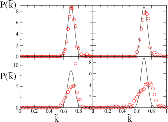
Figure 8: Solution of the inverse problem by the HMF equations in the presence of noise added to the external currents. We consider the same setup of Fig. 9 and we compare, for different values of the noise amplitude $\delta$, the reconstructed probability distribution $P(\tilde{k})$ (red circles) with the original gaussian distribution (black line): the upper–left panel corresponds to the noiseless case ($\delta=0$), while the upper–right, the lower–left and and the lower–right correspond to $\delta=0.1,0.2,0.3$, respectively.

As a matter of fact, the global neural activity fields obtained by experimental measurements are unavoidably affected by some level of noise. Accordingly, it is worth investigating the robustness of the inversion method also in the case of noise acting directly on $Y(t)$. In order to tackle this problem, we have considered a simple noisy version of the global synaptic activity field, defined as $Y_{\delta}(t)=(1+\eta(t))Y(t)$, where the random number $\eta(t)$ is uniformly extracted, at each integration time step, in the interval $[-\frac{\delta}{2},\frac{\delta}{2}]$. In Fig. 9 we show the distributions $P(\tilde{k})$ obtained for different values of $\delta$. We can conclude that the inversion method is quite stable with respect to this additive noise. In fact, even for very large signal–to–noise ratio (e.g. low–right panel of Fig. 9, where $\delta=0.8$) the main features of the original distribution are still recovered, within a reasonable approximation.

Figure 9: Solution of the inverse problem by the HMF equations in the presence of noise added to the activity field. We consider the same setup of Fig. 9, where now $a=1$ and $Y_{\delta}(t)=(1-\eta(t))Y(t)$ (the random variable $\eta(t)$ is extracted from a uniform probability distribution in the interval $[-\delta/2,\delta/2]$). We compare, for different values of the noise amplitude $\delta$, the reconstructed probability distribution $P(\tilde{k})$ (red circles) with the original gaussian distribution (black line): the upper–left, the upper–right, the lower–left and and the lower–right panels correspond to $\delta=0.1,0.4,0.8,1.2$, respectively.

VII HMF in sparse networks

In this section we analyze the effectiveness of the HMF approach for sparse networks, i.e. networks where the neurons degree does not scale linearly with $N$ and, in particular, the average degree $\langle k\rangle$ is independent of the system size. In this context, the coupling term describing the membrane potential of a generic neuron $i$, in a network of $N$ neurons, evolves according to the following equation:

$$\dot{v}_{j}=a-v_{j}+\frac{g}{\langle k\rangle}\sum_{i\neq j}\epsilon_{ij}y_{i},\,$$ (25)

while the dynamics of $y_{i}$ is the same of Eq.s (3)–(4). The coupling therm is now independent of $N$, and the normalization factor, $\langle k\rangle$, has been introduced in order to compare models with different average connectivity. The structure of the adjacency matrix $\epsilon_{ij}$ is determined by choosing for each neuron $i$ its in-degree $k_{i}$ from a probability distribution $P(k_{i})$ (with support over positive integers) independent of the system size.

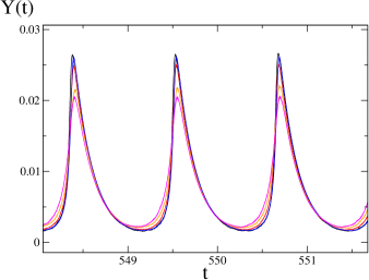
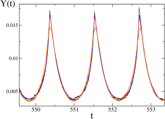
Figure 10: Comparison of the global synaptic activity field $Y(t)$ from sparse random networks with the same quantity generated by the corresponding HMF dynamics. We have considered sparse random networks with $N=10^{4}$ neurons. In the upper panel we consider a Gaussian probability distributions $P(k)$ with different averages $\langle k\rangle$ and variances $\sigma_{k}$, such that $\sigma_{k}/\langle k\rangle=0.06$: $\langle k\rangle=10,20,60,100$ correspond to the violet, orange, red and blue lines, respectively. The black line represents $Y(t)$ from the HMF dynamics ($M=10^{3}$), where $\hat{P}(\hat{k})$ is a Gaussian probability distribution with $\langle\hat{k}\rangle=1$ and $\sigma_{\hat{k}}=\sigma_{k}/\langle k\rangle=0.06$. In the lower panel we consider the scale free case with fixed power exponent $\alpha$ and different $k_{m}$: $k_{m}=10,30,70$ correspond to the orange, red and blue lines, respectively. The black line represents $Y(t)$ from the HMF dynamics ($M=10^{3}$), where $\hat{P}(\hat{k})=(\alpha-1)\hat{k}^{-\alpha}$ with cutoff $\hat{k}_{m}=1$.

On sparse networks the HMF model is not recovered in the thermodynamic limit, as the fluctuations of the field received by each neuron of in–degree $k_{i}$ do not vanish for $N\to\infty$. Nevertheless, for large enough values of $k_{i}$, one can expect that the fluctuations become negligible in such a limit, i.e. the synaptic activity field received by different neurons with the same in-degree is approximately the same. Eq. (25) can be turned into a mean–field like form as follows

$$\dot{v}_{j}=a-v_{j}+\frac{g}{\langle k\rangle}k_{j}Y~{},$$ (26)

where $Y(t)$ represents the global field, averaged over all neurons in the network. This implies that the equation is the same for all neurons with in–degree $k_{j}$, depending only on the ratio $\hat{k}_{j}=k_{j}/\langle k\rangle$. Consequently, also in this case one can read Eq. (26) as a HMF formulation of Eq. (25), where each class of neurons $\hat{k}$ evolves according to to Eq.s (10)–(13), with $\hat{k}$ replacing $\tilde{k}$, while the global activity field is given by the relation $Y(t)=\int_{0}^{\infty}\hat{P}(\hat{k})y_{\hat{k}}(t)d\hat{k}$.

In order to analyze the validity of the HMF as an approximation of models defined on sparse networks, we consider two main cases: (i) $\hat{P}(\hat{k})$ is a truncated Gaussian with average $\langle\hat{k}\rangle=1$ and standard deviation $\sigma_{\hat{k}}$; (ii) $\hat{P}(\hat{k})=(\alpha-1)\hat{k}^{-\alpha}$ is a power–law (i.e., scale free) distribution with a lower cutoff $\hat{k}_{m}=1$. The Gaussian case (i) is an approximation of any sparse model, where $P(k_{j})$ is a discretized Gaussian distribution with parameters $\langle k\rangle$ and $\sigma_{k}$, chosen in such a way that $\sigma_{\hat{k}}=\sigma_{k}/\langle k\rangle$. The scale free case (ii) approximates any sparse model, where $P(k_{j})$ is a power law with exponent $\alpha$ and a generic cutoff. Such an approximation is expected to provide better results the larger is $\langle k\rangle$, i.e. the larger is the cutoff $k_{m}$ of the scale free distribution. In Fig. 10 we plot the global field emerging from the HMF model, superposing those coming from a large finite size realization of the sparse network, with different values of $\langle k\rangle$ for the Gaussian case (upper panel) and of $k_{m}$ for the scale free case (lower panel). The HMF equations exhibit a remarkable agreement with models on sparse network, even for relatively small values of $\langle k\rangle$ and $k_{m}$. This analysis indicates that the HMF approach works also for non–massive topologies, provided the typical connectivities in the network are large enough, e.g. $\langle k\rangle\sim{\mathcal{O}}(10^{2})$ in a Gaussian random network with $N=10^{4}$ neurons (see Fig. (10)).

VIII Conclusions

For systems with a very large number of components, the effectiveness of a statistical approach, paying the price of some necessary approximation, has been extensively proven, and mean–field methods are typical in this sense. In this paper we discuss how such a method, in the specific form of Heterogeneous Mean–Field, can be defined in order to fit an effective description of neural dynamics on random networks.

The relative simplicity of the model studied here, excitatory leaky–integrate–and fire neurons with short term synaptic plasticity, is also a way of providing a pedagogical description of the HMF and of its potential interest in similar contexts BCDLV .

We have reported a detailed study of the HMF approach including investigations on (i) its stability properties, (ii) its effectiveness in describing the dynamics and in solving the associated inverse problem for different network topologies, (iii) its robustness with respect to noise, and (iv) its adaptability to different formulations of the model at hand. In the light of (ii) and (iii), the HMF approach appears quite a promising tool to match experimental situations, such as the identification of topological features of real neural structures, through the inverse analysis of signals extracted as time series from small, but not microscopic, domains. On a mathematical ground, the HMF approach is a simple and effective mean–field formulation, that can be extended to other neural network models and also to a wider class of dynamical models on random graphs. The first step in this direction could be the extension of the HMF method to the more interesting case, where the random network contains excitatory and inhibitory neurons, according to distributions of interest for neurophysiology abeles ; bonif . This will be the subject of our future work.

- (1) D. de Santos-Sierra, I. Sendi a-Nadal, I. Leyva, J. A. Almendral, S. Anava, A. Ayali, D. Papo, and S. Boccaletti, PLoS ONE 9(1): e85828 (2014).
- (2) V. Volman, I. Baruchi, E. Persi and E. Ben-Jacob, Physica A 335, 249 (2004).
- (3) Hidalgo J, Seoane LF, Cort s JM, Muoz MA, PLoS ONE 7(8), e40710 (2012).
- (4) J. F. Mejias, H. J. Kappen and J. J. Torres, PLoS ONE 5(11), e13651 (2010)
- (5) N. Brunel, Journal of computational neuroscience, 8(3), 183-208 (2000).
- (6) L. Calamai, A. Politi, A. Torcini, Phys. Rev. E 80, 036209 (2009)
- (7) D. Millman, S. Mihalas, A. Kirkwood & E. Niebur, Nature physics, 6(10), 801-805 (2010).
- (8) B. Cessac, B. Doyon, M. Quoy M. & Samuelides, Physica D: Nonlinear Phenomena, 74(1), 24-44 (1994).
- (9) P.C. Bressloff, Phys. Rev. E, 60(2), 2160 (1999).
- (10) A. Barrat, M. Barthelemy, and A. Vespignani, Dynamical Processes on Complex Networks, Cambridge University Press, Cambridge, UK (2008).
- (11) S. N. Dorogovtsev, A.V. Goltsev, and J. F. F. Mendes, Rev. Mod. Phys. 80, 1275 (2008).
- (12) M. di Volo, R. Livi, S. Luccioli, A. Politi and A. Torcini, Phys. Rev. E 87, 032801 (2013).
- (13) R. Burioni, M. di Volo, M. Casartelli, R. Livi and A. Vezzani, Scientific Reports 4, 4336 (2014).
- (14) M. Tsodyks and H. Markram, Proc. Natl. Acad. Sci. USA 94, 719 (1997).
- (15) M. Tsodyks, K. Pawelzik and H. Markram, Neural Comput. 10, 821, (1998).
- (16) M. Tsodyks, A. Uziel and H. Markram, The Journal of Neuroscience 20, RC1 (1-5) (2000).
- (17) R. Brette, Neural Comput. 18, 2004 (2006).
- (18) R. Zillmer, R. Livi, A. Politi, and A. Torcini, Phys. Rev. E 76, 046102 (2007).
- (19) M. di Volo and R. Livi, J. of Chaos Solitons and Fractals 57, 54–61 (2013).
- (20) M. Tsodyks, I. Mitkov, and H. Sompolinsky, Phys. Rev. Lett. 71, 1280 (1993).
- (21) G. Benettin, L. Galgani, A. Giorgilli and J.-M. Strelcyn, Meccanica 15, 21 (1980).
- (22) R. Kress, Linear Integral equations Applied numerical sciences, v.82, Springer-Verlag, New York, (1999).
- (23) Abeles, Corticonics. New York: Cambridge UP (1991).
- (24) P. Bonifazi, M. Goldin, M. A. Picardo, I. Jorquera, A. Cattani, G. Bianconi & R. Cossart, Science, 326(5958), 1419-1424 (2009).