Phase Diagram in Stored-Energy-Driven Lévy Flight

Abstract

Phase diagram based on the mean square displacement (MSD) and the distribution of diffusion coefficients of the time-averaged MSD for the stored-energy-driven Lévy flight (SEDLF) is presented. In the SEDLF, a random walker cannot move while storing energy, and it jumps by the stored energy. The SEDLF shows a whole spectrum of anomalous diffusions including subdiffusion and superdiffusion, depending on the coupling parameter between storing time (trapping time) and stored energy. This stochastic process can be investigated analytically with the aid of renewal theory. Here, we consider two different renewal processes, i.e., ordinary renewal process and equilibrium renewal process, when the mean trapping time does not diverge. We analytically show the phase diagram according to the coupling parameter and the power exponent in the trapping-time distribution. In particular, we find that distributional behavior of time-averaged MSD intrinsically appears in superdiffusive as well as normal diffusive regime even when the mean trapping time does not diverge.

I Introduction

In normal diffusion processes, the diffusivity can be characterized by the diffusion coefficient in the mean square displacement (MSD). However, many diffusion processes in nature show anomalous diffusion; that is, the MSD does not grow linearly with time but follows a sublinear or superlinear growth with time,

$$\langle x_{t}^{2}\rangle\propto t^{\beta}\quad(\beta\neq 1),$$ (1)

where $x_{t}$ is a position in one-dimensional coordinate, $t$ is time, and $\langle\cdot\rangle$ means an ensemble average. In particular, anomalous diffusion in biological systems has been found by single-particle tracking experiments Caspi2000 (1, 2, 3, 4, 5, 6, 7). Thus, the power-law exponent $\beta$ is one of the most important quantities characterizing the underlying diffusion process. Especially, anomalous diffusion with $\beta<1$ is called subdiffusion and that with $\beta>1$ is called superdiffusion.

Although anomalous diffusion can be characterized by the power-law exponent $\beta$ in the MSD, the exponent cannot reveal the underlying physical nature in itself. This is because the same power-law exponent in the MSD does not imply that the physical mechanism in the anomalous diffusion is also the same. Therefore, clarifying the origin of anomalous diffusion is an important subject, and many researches on this issue have been conducted extensively Magdziarz2009 (8, 9, 10, 11, 12). One of the key properties characterizing anomalous diffusion is ergodicity, i.e., time-averaged observables being equal to a constant (the ensemble average). In some experiments Golding2006 (2, 3, 4, 5, 7), (generalized) diffusion coefficients for time-averaged MSDs show large fluctuations, suggesting that ergodicity breaks.

In stochastic models of anomalous diffusion, continuous-time random walk (CTRW) shows a prominent feature called distributional ergodicity Lubelski2008 (13, 14, 15, 16); that is, the time-averaged observables obtained from single trajectories do not converge to a constant but the distribution of such time-averaged observables converges to a universal distribution (convergence in distribution). More precisely, the distribution of the time-averaged MSD (TAMSD), which is defined by

$$\overline{\delta^{2}(\Delta;t)}\equiv\frac{1}{t-\Delta}\int_{0}^{t-\Delta}(x_{t^{\prime}+\Delta}-x_{t^{\prime}})^{2}dt^{\prime},$$ (2)

converges to the Mittag-Leffler distribution of order $\alpha$ He2008 (14, 17). This statement can be represented by

$$\frac{\overline{\delta^{2}(\Delta;t)}}{\langle\overline{\delta^{2}(\Delta;t)}\rangle}\Rightarrow M_{\alpha}\quad{\rm as}~{}t\to\infty,$$ (3)

for a fixed $\Delta$ ($\ll t$), where $M_{\alpha}$ is a random variable with the Mittag-Leffler distribution of order $\alpha$. We note that the diffusion coefficients in the TAMSDs are also distributed according to the Mittag-Leffler distribution because the TAMSD shows normal diffusion, i.e, $\overline{\delta^{2}(\Delta;t)}\simeq D_{t}\Delta$ Miyaguchi2011a (15, 16), where we refer to $D_{t}$ as the diffusion coefficient. In stochastic models, such distributional behavior originates from the divergent mean trapping time. In diffusion in a random energy landscape such as a trap model bouchaud90 (18), the trapping-time distribution follows a power law, $w(\tau)\propto\tau^{-1-\alpha}$, if heights of the energy barrier are distributed according to the exponential distribution. The exponent $\alpha$ smaller than 1 implies a divergence of the mean. In dynamical systems, this divergent mean brings an infinite measure Akimoto2010a (19). Thus, such distributional behavior of time-averaged observables is also shown in infinite ergodic theory Akimoto2010 (17, 20). Moreover, large fluctuations of time-averaged observables, related to distributional ergodicity, have been observed in biological experiments Golding2006 (2, 3, 4, 5, 7) as well as quantum dot experiments Brok2003 (21, 22).

Recently, we have shown that the distribution of the diffusion coefficients of the TAMSDs in the stored-energy-driven Lévy flight (SEDLF) is different from that in CTRW Akimoto2013a (23). The SEDLF is a CTRW with jump lengths correlated with trapping times Klafter1987 (24, 25, 26). One of the most typical examples for such a correlated motion can be observed in Lévy walk Shlesinger1987 (27). However, Lévy walk and SEDLF are completely different stochastic processes in that a random walker cannot move while it is traped in SEDLF, whereas it can move with constant velocity in Lévy walk. In other words, in SEDLF, a random walker does not move while storing a sort of energy, and it jumps using the stored energy (see Fig. 1). When the trapping-time distribution follows a power-law, the jump length distribution also follows a power-law, the same as in Lévy flight. Since we consider a power-law trapping-time distribution, we refer to our model as the stored-energy-driven Lévy flight. We note that the MSD does not diverge in SEDLF, whereas it always diverges in Lévy flight. Although the ensemble-averaged MSDs show subdiffusion as well as superdiffusion, the TAMSDs always increase linearly with time in SEDLF Akimoto2013a (23). This behavior is completely different from that in Lévy walk Akimoto2012 (28, 29). Moreover, the distribution of the TAMSD with a fixed $\Delta$ converge to a time-independent distribution which is not the same as a universal distribution in CTRW (Mittag-Leffler distribution):

$$\frac{\overline{\delta^{2}(\Delta;t)}}{\langle\overline{\delta^{2}(\Delta;t)}\rangle}\Rightarrow Y_{\alpha,\gamma}\quad{\rm as}~{}t\to\infty,$$ (4)

where $Y_{\alpha,\gamma}$ is a random variable and $\gamma$ is the coupling parameter between trapping time and jump length. We note that such coupling effects become physically important in turbulent diffusion Shlesinger1987 (27), diffusion of cold atoms Barkai2014 (30), and nonthermal systems such as cells Caspi2000 (1, 6). In such enhanced diffusions, it has been known that the coupling between jump lengths and waiting times follows a power-law fashion like SEDLF Shlesinger1987 (27, 30), although a particle is always moving, which is different from SEDLF. Furthermore, it will also be important in complex systems such as finance Meerschaert2006 (31) and earthquakes Corral2006 (32, 33) because jump lengths are correlated with the waiting times in such systems.

In terms of an ensemble average, SEDLF exhibits a whole spectrum of diffusion: sub-, normal-, and super-diffusion, depending on the coupling parameter Akimoto2013a (23, 24, 25, 26). Because distributional behavior of the time-averaged observables such as the diffusion coefficients in SEDLF is different from that in CTRW, it is important to construct a phase diagram in terms of the power-law exponent of the MSD as well as the form of the distribution function of the TAMSD. Here, we provide the phase diagram for the whole parameters range in SEDLF.

II Model

SEDLF is a cumulative process, which is a generalization of a renewal process Cox (34). Equivalently, SEDLF is a CTRW with a non-separable joint probability of trapping time and jump length. Therefore, the SEDLF can be defined through the joint probability density function (PDF) $\psi(x,t)$, where $\psi(x,t)dxdt$ is the probability that a random walker jumps with length $[x,x+dx)$ just after it is trapped for period $[t,t+dt)$ since its previous jump bouchaud90 (18, 35). Here, we consider the following joint PDF

$$\psi(x,t)=w(t)\frac{\delta(x-t^{\gamma})+\delta(x+t^{\gamma})}{2},$$ (5)

where $w(t)$ is the PDF of trapping times and $0\leq\gamma\leq 1$ is a coupling strength. This kind of coupling has been introduced in Klafter1987 (24, 35). The SEDLF with $\gamma=0$ is just a separable CTRW. In addition, we consider that the PDF of trapping times follows a power law:

$$w(t)\simeq\frac{c_{0}}{t^{1+\alpha}},$$ (6)

as $t\to\infty$. Here, $\alpha\in(0,2)$ is the stable index, a constant $c_{0}$ is defined by $c_{0}={c}/{|\Gamma(-\alpha)|}$ with a scale factor $c$. We note that the mean trapping time diverges for $\alpha\leq 1$. For $\gamma>0$, the PDF of jump length also follows a power law:

$$l(x)=\int_{0}^{\infty}\psi(x,t)dt=\frac{|x|^{\frac{1}{\gamma}-1}}{2\gamma}w\left(|x|^{\frac{1}{\gamma}}\right)\simeq\frac{c_{0}}{2\gamma}\frac{1}{|x|^{1+{\alpha}/{\gamma}}}.$$ (7)

Thus, the second moment of the jump length diverges for $2\gamma\geq\alpha$. Because Lévy flight also has a power law distribution of jump length, we call this random walk the stored-energy-driven Lévy flight. In numerical simulations, we set the PDF of the trapping time as $w(t)=\alpha t^{-1-\alpha}$ $(t\geq 1)$. Thus, the jump length PDF is given by $l(x)=\alpha/(2\gamma|x|^{1+\alpha/\gamma})$ from Eq. (7), and $\langle l^{2}\rangle=\alpha/(\alpha-2\gamma)$ for $2\gamma<\alpha$.

Because the mean trapping time is finite for $\alpha>1$, we consider two typical renewal processes; ordinary renewal process and equilibrium renewal process Cox (34). Equilibrium renewal process is assumed to start $-t_{a}=-\infty$ (see Fig. 1). The PDF of the first jump length $x$ and the first apparent trapping time (the forward recurrence time) $t$, $\psi_{0}(x,t)$, is given by

$$\psi_{0}(x,t)=\frac{1}{\mu}\int_{t}^{\infty}w(t^{\prime})\frac{\delta(x-t^{\prime\gamma})+\delta(x+t^{\prime\gamma})}{2}dt^{\prime},$$ (8)

where $\mu$ is the mean trapping time. See Appendix A for the derivation. Generally, the first (true) trapping time is longer than the first apparent trapping time. Integrating Eq. (8) in terms of $x$, we have the PDF of the first apparent trapping time:

$$w_{0}(t)=\frac{1}{\mu}\int_{t}^{\infty}w(t^{\prime})dt^{\prime}.$$ (9)

Note that the Eq. (9) is consistent with the result obtained in renewal theory, i.e., the PDF of the forward recurrence time Cox (34). Thus, the joint PDF of the first jump length and the first apparent trapping time, $\psi_{0}(x,t)$, is not given by the form in Eq. (5). This is because the first jump length $x$ is determined by the time elapsed since a random walker’s last jump (the first true trapping time) and thus it is not directly related to the first apparent trapping time, i.e., the time elapsed since the beginning of the measurement at $t=0$. For ordinary renewal process, we just set $w_{0}(t)=w(t)$ and $\psi_{0}(x,t)=\psi(x,t)$. For $\alpha\leq 1$, we only consider an ordinary renewal process because there is no equilibrium ensemble due to divergent mean trapping time which causes aging Barkai2003 (36, 37, 38).

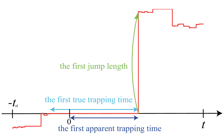
Figure 1: Trajectory of SEDLF in an equilibrium renewal process. A measurement starts at $t=0$ while the process starts at $-t_{a}$. An equilibrium process means a process with $t_{a}\to\infty$ if there exist an equilibrium distribution for the first apparent time and the second moment of the first jump length.

III Generalized Renewal Equation

The spacial distribution $P(x,t)$ of CTRWs with starting from the origin satisfies the generized renewal equations:

$$P(x,t) =\int_{0}^{t}dt^{\prime}\Psi(t-t^{\prime})Q(x,t^{\prime})+\Psi_{0}(t)\delta(x),$$ (10)

$$Q(x,t) =\int_{-\infty}^{\infty}dx^{\prime}\int_{0}^{t}dt^{\prime}\psi(x^{\prime},t^{\prime})Q(x-x^{\prime},t-t^{\prime})$$

$$\quad+\psi_{0}(x,t),$$ (11)

where $Q(x,t)dtdx$ is the probability of a random walker reaching an interval $[x,x+dx)$ just in a period $[t,t+dt)$, and $\Psi(t)$ [$\Psi_{0}(t)$] is the probability of being trapped for longer than time $t$ just after a renewal (after the measurement starts at $t=0$). $\Psi(t)$ and $\Psi_{0}(t)$ are defined as follows:

$$\Psi(t) =1-\int_{-\infty}^{\infty}dx^{\prime}\int_{0}^{t}\psi(x^{\prime},t^{\prime})dt^{\prime}=1-\int_{0}^{t}w(t^{\prime})dt^{\prime},$$ (12)

$$\Psi_{0}(t) =1-\int_{-\infty}^{\infty}dx^{\prime}\int_{0}^{t}\psi_{0}(x^{\prime},t^{\prime})dt^{\prime}=1-\int_{0}^{t}w_{0}(t^{\prime})dt^{\prime}.$$ (13)

Then, the Laplace transforms of these functions are given by

$$\hat{\Psi}(s)=\frac{1-\hat{w}(s)}{s},\qquad\hat{\Psi}_{0}(s)=\frac{\mu s-1+\hat{w}(s)}{\mu s^{2}}.$$ (14)

In an ordinary renewal process, $\psi_{0}(x,t)$ is the same as $\psi(x,t)$. On the other hand, the first jump length $x$ is not determined by the first apparent trapping time $t$ in an equilibrium renewal process, while the first jump length is not independent of the first apparent trapping time. Fourier-Laplace transform with respect to space and time ($x\rightarrow k$ and $t\rightarrow s$, respectively), defined by

$${\hat{P}}(k,s)\equiv\int_{-\infty}^{\infty}dx\int_{0}^{\infty}dtP(x,t)e^{ikx}e^{-st},$$ (15)

gives

$${\hat{P}}(k,s) = \frac{\hat{\Psi}(s)\hat{\psi}_{0}(k,s)+\hat{\Psi}_{0}(s)[1-\hat{\psi}(k,s)]}{1-{\hat{\psi}}(k,s)},$$ (16)

where $\hat{\psi}_{0}(k,s)$ and $\hat{\psi}(k,s)$ are Fourier-Laplace transforms of ${\psi}_{0}(x,t)$ and ${\psi}(x,t)$, respectively. In what follows, we use the notations $P^{o}(x,t)$ and $\hat{P}^{o}(k,s)$ for the ordinary renewal process, and $P^{eq}(x,t)$ and $\hat{P}^{eq}(k,s)$ for the equilibrium renewal process.

For ordinary renewal process, i.e., $\psi_{0}(t)=\psi(t)$ and $\Psi_{0}(t)=\Psi(t)$, we have the following generalized renewal equation in the Fourier and Laplace space:

$${\hat{P}}^{o}(k,s)=\frac{1}{s}\frac{1-\hat{w}(s)}{1-{\hat{\psi}}(k,s)},$$ (17)

where we used Eq. (14). For equilibrium renewal process ($\alpha>1$), we have

$${\hat{P}}^{eq}(k,s) =\frac{1}{s}-\frac{1-\hat{w}(s)}{\mu s^{2}}\frac{1-\hat{\psi}(k,0)}{1-{\hat{\psi}}(k,s)},$$ (18)

where we used Eq. (14) and

$$\hat{\psi}_{0}(k,s)=\frac{\hat{\psi}(k,0)-\hat{\psi}(k,s)}{\mu s}.$$ (19)

The derivation of Eq. (19) is shown in Appendix A.

Thus we expressed $\hat{P}^{o}(k,s)$ and $\hat{P}^{eq}(k,s)$ with $\hat{\psi}(k,t)$ and $\hat{w}(s)$ [Eqs. (17) and (18)]. Now, we derive the explicit forms of these functions. From Eq. (5), ${\hat{\psi}}(k,s)$ is given by

$${\hat{\psi}}(k,s)=\int_{0}^{\infty}e^{-st}\cos\left(kt^{\gamma}\right)w(t)dt.$$ (20)

Note that ${\hat{\psi}}(0,s)=\hat{w}(s)$. In addition, from Eq. (6), the asymptotic behavior of the Laplace transform $\hat{w}(s)$ for $s\rightarrow 0$ is given by

$$\hat{w}(s)=\begin{cases}1-cs^{\alpha}+o(s^{\alpha}),\quad&(0<\alpha<1)\\[8.5359pt] 1+c_{0}s\ln s+o(s\ln s),\quad&(\alpha=1)\\[8.5359pt] 1-\mu s+cs^{\alpha}+o(s^{\alpha}),\quad&(1<\alpha<2)\end{cases}$$

where $\mu=\left\langle t\right\rangle=\int_{0}^{\infty}tw(t)dt$.

IV Mean Square Displacement

The asymptotic behavior of the moments of position $x_{t}$ for $t\rightarrow\infty$ can be obtained using the Fourier-Laplace transform $\hat{P}(k,s)$. Because $\left.\frac{\partial{\hat{P}}(k,s)}{\partial k}\right|_{k=0}=0$, $\langle x_{t}\rangle=0$ for both renewal processes.

In ordinary renewal process, the Laplace transform of the second moment, i.e., the ensemble-averaged MSD (EAMSD), is given by

$$\langle x^{2}_{s}\rangle_{o} = \left.-\frac{\partial^{2}{\hat{P}}^{o}(k,s)}{\partial k^{2}}\right|_{k=0}=-\frac{1}{s}\frac{{\hat{\psi}}^{\prime\prime}(0,s)}{1-{\hat{w}}(s)},$$ (21)

where the ensemble average $\langle\ldots\rangle_{o}$ is taken with respect to an ordinary renewal process. For $\alpha\in(0,1)$, we obtain the EAMSD Akimoto2013a (23):

$$\langle x^{2}_{t}\rangle_{o}\simeq\begin{cases}\dfrac{\left\langle l^{2}\right\rangle}{c\Gamma(1+\alpha)}t^{\alpha},&\quad\left(0<2\gamma<\alpha\right)\\[14.22636pt] \dfrac{1}{|\Gamma(-\alpha)|\Gamma(1+\alpha)}t^{\alpha}\log t,&\quad\left(2\gamma=\alpha\right)\\[14.22636pt] \dfrac{\Gamma(2\gamma-\alpha)}{|\Gamma(-\alpha)|\Gamma(1+2\gamma)}t^{2\gamma},&\quad\left(\alpha<2\gamma\leq 2\right)\end{cases}$$ (22)

where we used $\left\langle t^{2\gamma}\right\rangle=\left\langle l^{2}\right\rangle=\int_{-\infty}^{\infty}x^{2}l(x)dx$ when $\langle l^{2}\rangle<\infty$.

For $\alpha=1$, the EAMSD is given by

$$\langle x^{2}_{t}\rangle_{o}\simeq\begin{cases}\dfrac{\left\langle l^{2}\right\rangle}{c_{0}}\dfrac{t}{\log t},&\quad\left(0<2\gamma<1\right)\\[14.22636pt] t,&\quad\left(2\gamma=1\right)\\[8.5359pt] \dfrac{\Gamma(2\gamma-1)}{\Gamma(2\gamma+1)}\dfrac{t^{2\gamma}}{\log t},&\quad\left(1<2\gamma\leq 2\right)\end{cases}$$ (23)

Finally, for $\alpha\in(1,2)$, the EAMSD is given by

$$\langle x^{2}_{t}\rangle_{o}\simeq\begin{cases}\frac{\left\langle l^{2}\right\rangle}{\mu}t\left[1+\frac{ct^{1-\alpha}}{\mu\Gamma(3-\alpha)}\right],&\left(0<2\gamma<1\right)\\[14.22636pt] \frac{\left\langle l^{2}\right\rangle}{\mu}t+\frac{ct^{2-\alpha}}{\mu\Gamma(3-\alpha)}\left[\frac{\left\langle l^{2}\right\rangle}{\mu}-\alpha\right],&\left(2\gamma=1\right)\\[14.22636pt] \frac{\left\langle l^{2}\right\rangle}{\mu}t+\frac{c_{0}}{\mu}\frac{\Gamma(2\gamma-\alpha)}{\Gamma(2\gamma-\alpha+2)}t^{2\gamma-\alpha+1},&\left(1<2\gamma<\alpha\right)\\[14.22636pt] \frac{c_{0}}{\mu}t\log t,&\left(2\gamma=\alpha\right)\\[14.22636pt] \frac{c_{0}\Gamma(2\gamma-\alpha)}{\mu\Gamma(2\gamma-\alpha+2)}t^{2\gamma-\alpha+1}.&\left(\alpha<2\gamma\leq 2\right)\end{cases}$$ (24)

These results are consistent with a previous study Klafter1987 (24). We note that the EAMSD for $\gamma=1$ is smaller than that in Lévy walk, whereas the scaling exponent $3-\alpha$ is the same as that in Lévy walk Zumofen1993 (39). This is because SEDLF is a wait and jump model, while Lévy walk is a moving model.

In equilibrium renewal process ($\alpha>1$),

$$\langle x^{2}_{s}\rangle_{eq} =\left.-\frac{\partial^{2}{\hat{P}}^{\rm eq}(k,s)}{\partial k^{2}}\right|_{k=0}=\frac{\hat{\psi}^{\prime\prime}(0,0)}{\mu s^{2}}.$$ (25)

Eq. (25) is valid only for $0<2\gamma<\alpha-1$, otherwise the second moment of the first jump length diverges, i.e., the EAMSD diverges. This is very different from Lévy walk process because there exists an equilibrium renewal process in Lévy walk with $\alpha>1$. Because $\hat{\psi}^{\prime\prime}(0,0)=\left\langle l^{2}\right\rangle$ for $0<2\gamma<\alpha-1$, the EAMSD is given by

$$\langle x^{2}_{t}\rangle_{eq}=\frac{\langle l^{2}\rangle}{\mu}t.$$ (26)

In SEDLF, the leading order of the EAMSD in an ordinary renewal process is the same as that in an equilibrium renewal process ($\alpha>2\gamma+1$). On the other hand, in Lévy walk, the proportional constant of the EAMSD in a non-equilibrium ensemble such as an ordinary renewal process differs from that in an equilibrium one Froemberg2013 (29, 39, 40, 41). We note that the TAMSD coincides with the EAMSD in an equilibrium ensemble as the measurement time goes to infinity. Significant initial ensemble dependence of statistical quantity has been also observed in non-hyperbolic dynamical systems Akimoto2007 (42).

V Time-averaged Mean Square Displacement

In normal Brownian motion, the TAMSD defined by Eq. (2) converges to the MSD with an equilibrium ensemble:

$$\overline{\delta^{2}(\Delta;t)}\rightarrow{\color[rgb]{0,0,0}\langle x_{\Delta}^{2}\rangle_{eq}}~{}{\rm as}~{}t\to\infty.$$ (27)

Such ergodic property does not hold in various stochastic models of anomalous diffusion such as CTRW and Lévy walk Lubelski2008 (13, 14, 29). Here, we derive the TAMSD in the SEDLF. In wait and jump random walks with random waiting times such as CTRW and SEDLF, the TAMSD can be represented using the total number of jumps, denoted by $N_{t}$, and $h_{k}=\Delta l_{k}^{2}+2\sum_{m=1}^{k-1}l_{k}l_{m}\theta(\Delta-t_{k}+t_{m})$ Miyaguchi2011a (15, 23, 43):

$$\overline{\delta^{2}(\Delta;t)}\simeq\frac{1}{t}\sum_{k=0}^{N_{t}}h_{k}\quad(t\rightarrow\infty),$$ (28)

where $l_{k}$ is the $k$-th jump length, $t_{k}$ is the time when the $k$-th jump occurs, and $\theta(t)$ is a step function, defined by $\theta(t)=0$ for $t<0$ and $t$ otherwise. For $\gamma>0$, one can show that $\sum_{k=0}^{N_{t}}(h_{k}-\Delta l^{2}_{k})/\sum_{k=0}^{N_{t}}l_{k}^{2}\rightarrow 0$ as $t\rightarrow\infty$ Akimoto2013a (23). Therefore, the TAMSD can be written as

$$\overline{\delta^{2}(\Delta;t)}\simeq D_{t}\Delta\quad(\Delta\ll t~{}{\rm and}~{}t\rightarrow\infty),$$ (29)

where $D_{t}=\sum_{k=0}^{N_{t}}l^{2}_{k}/t$. We note that the relation (28) does not hold if the random walker moves with constant speed as in Lévy walk because $(x_{t+\Delta}-x_{t})^{2}$ is simply zero in SEDLF but not in Lévy walk. In fact, the TAMSD does not increase linearly with time in Lévy walk Froemberg2013 (29, 40, 41).

To investigate an ergodic property of the time-averaged diffusion coefficient $D_{t}$, we derive the PDF $P_{2}(z,t)$ of $Z_{t}\equiv\sum_{k=0}^{N_{t}}l^{2}_{k}$. Because $l^{2}_{k}$ and $N_{t}$ are mutually correlated, we use the generalized renewal equation for $Z_{t}$:

$$P_{2}(z,t) =\int_{0}^{t}dt^{\prime}\Psi(t-t^{\prime})Q_{2}(z,t^{\prime})+\Psi_{0}(t)\delta(z),$$ (30)

$$Q_{2}(z,t) =\int_{0}^{\infty}dz^{\prime}\int_{0}^{t}dt^{\prime}\phi(z^{\prime},t^{\prime})Q_{2}(z-x^{\prime},t-t^{\prime})$$

$$\quad+\phi_{0}(z,t),$$ (31)

where the joint PDF $\phi(z,t)$ is given by

$$\phi(z,t)=w(t)\delta(z-t^{2\gamma})$$ (32)

The joint PDF of the first squared jump length $z=l_{0}^{2}$ and apparent trapping time $t$, $\phi_{0}(z,t)$, is given by $\phi_{0}(z,t)=\phi(z,t)$ for the ordinary ensemble, whereas

$$\phi_{0}(z,t)=\frac{1}{\mu}\int_{t}^{\infty}dt^{\prime}w(t^{\prime})\delta(z-t^{\prime 2\gamma}),$$ (33)

for equilibrium ensemble, which can be derived in the same way as the derivation of $\psi_{0}(x,t)$ given in Appendix A. The double Laplace transform with respect to $z$ and time $t$ is defined by

$${\hat{P}}_{2}(k,s)\equiv\int_{0}^{\infty}dz\int_{0}^{\infty}dtP_{2}(z,t)e^{-kz}e^{-st}.$$ (34)

From the generalized renewal equations (30) and (V), we obtain

$${\hat{P}}_{2}(k,s)=\frac{\hat{\Psi}(s)\hat{\phi}_{0}(k,s)+\hat{\Psi}_{0}(s)[1-\hat{\phi}(k,s)]}{1-{\hat{\phi}}(k,s)},$$ (35)

where the double Laplace transform of $\phi(z,t)$ is given by

$$\hat{\phi}(k,s)=\int_{0}^{\infty}e^{-st}e^{-kt^{2\gamma}}w(t)dt,$$ (36)

and that of $\phi_{0}(z,t)$ is given by $\phi_{0}(z,t)=\phi(z,t)$ for the ordinary process, and by

$$\hat{\phi}_{0}(k,s) =\frac{\hat{\phi}(k,0)-\hat{\phi}(k,s)}{\mu s},$$ (37)

for the equilibrium process. Note that $\hat{\phi}(0,s)=\hat{w}(s)$.

V.1 Ordinary Renewal Process

In ordinary renewal process, the Laplace transform ${\hat{P}_{2}}^{o}(k,s)$ is given by

$${\hat{P}_{2}}^{o}(k,s)=\frac{1}{s}\frac{1-\hat{w}(s)}{1-{\hat{\phi}}(k,s)}.$$ (38)

Thus, we have the Laplace transform of $\langle Z_{t}\rangle_{o}$ as follows:

$$\langle Z_{s}\rangle_{o}=\left.-\frac{\partial\hat{P}^{o}_{2}(k,s)}{\partial k}\right|_{k=0}=\frac{-\hat{\phi}^{\prime}(0,s)}{s[1-\hat{w}(s)]}=\left\langle x_{s}^{2}\right\rangle_{o},$$ (39)

where we used $-\hat{\phi}^{\prime}(0,s)=-\hat{\psi}^{\prime\prime}(0,s)$ and Eq. (21). Then, averaging Eq. (29) over an ordinary ensemble, we have

$$\langle\overline{\delta^{2}(\Delta;t)}\rangle_{o}\simeq\left\langle D_{t}\right\rangle_{o}\Delta=\frac{\langle x_{t}^{2}\rangle_{o}}{t}\Delta$$ (40)

Therefore, using Eqs. (22)–(24), we have the leading terms of the mean diffusion coefficient, $\langle D_{t}\rangle_{o}=\langle x_{t}^{2}\rangle_{o}/t$, for $t\rightarrow\infty$ as follows:

$$\langle D_{t}\rangle_{o} \simeq\begin{cases}\frac{\left\langle l^{2}\right\rangle}{c\Gamma(1+\alpha)}t^{\alpha-1}&\left(0<2\gamma<\alpha\right)\\[8.5359pt] \frac{1}{|\Gamma(-\alpha)|\Gamma(1+\alpha)}t^{\alpha-1}\log t&\left(2\gamma=\alpha\right)\\[8.5359pt] \frac{\Gamma(2\gamma-\alpha)}{|\Gamma(-\alpha)|\Gamma(1+2\gamma)}t^{2\gamma-1}&\left(\alpha<2\gamma\leq 2\right)\end{cases}$$ (41)

for $0<\alpha<1$,

$$\langle D_{t}\rangle_{o}\simeq\begin{cases}\frac{\left\langle l^{2}\right\rangle}{c_{0}}\frac{1}{\log t}+o\left(\frac{1}{\log t}\right).&\quad\left(0<2\gamma<1\right)\\[8.5359pt] 1+O\left(\frac{1}{\log t}\right),&\quad\left(2\gamma=1\right)\\[8.5359pt] \frac{\Gamma(2\gamma-1)}{\Gamma(2\gamma+1)}\frac{t^{2\gamma-1}}{\log t},&\quad\left(1<2\gamma\leq 2\right)\end{cases}$$ (42)

for $\alpha=1$, and

$$\langle D_{t}\rangle_{o}\simeq\begin{cases}\frac{\left\langle l^{2}\right\rangle}{\mu}\left[1+\frac{ct^{1-\alpha}}{\mu\Gamma(3-\alpha)}\right],&\left(0<2\gamma<1\right)\\[8.5359pt] \frac{\left\langle l^{2}\right\rangle}{\mu}+\frac{ct^{1-\alpha}}{\mu\Gamma(3-\alpha)}\left[\frac{\left\langle l^{2}\right\rangle}{\mu}-\alpha\right],&\left(2\gamma=1\right)\\[8.5359pt] \frac{\left\langle l^{2}\right\rangle}{\mu}+\frac{c_{0}}{\mu}\frac{\Gamma(2\gamma-\alpha)}{\Gamma(2\gamma-\alpha+2)}t^{2\gamma-\alpha},&\left(1<2\gamma<\alpha\right)\\[8.5359pt] \frac{c_{0}}{\mu}\log t,&\left(2\gamma=\alpha\right)\\[8.5359pt] \frac{c_{0}\Gamma(2\gamma-\alpha)}{\mu\Gamma(2\gamma-\alpha+2)}t^{2\gamma-\alpha}&\left(\alpha<2\gamma\leq 2\right)\end{cases}$$ (43)

for $1<\alpha<2$. It follows that the mean diffusion coefficient diverges as $t$ goes to infinity for $1<\alpha<2$ and $\alpha<2\gamma<2$.

Similarly, the Laplace transform of $\langle Z_{t}^{2}\rangle$ is given by

$$\langle Z_{s}^{2}\rangle_{o}=\frac{1}{s[1-\hat{w}(s)]}\left\{\frac{2\hat{\phi}^{\prime}(0,s)^{2}}{1-\hat{w}(s)}+\hat{\phi}^{\prime\prime}(0,s)\right\}.$$ (44)

It follows that the leading order of the second moment of $D_{t}$ is given by

$$\langle D^{2}_{t}\rangle_{o}\simeq\begin{cases}\frac{2\left\langle l^{2}\right\rangle^{2}}{c^{2}\Gamma(2\alpha+1)}t^{2(\alpha-1)},&(0<2\gamma<\alpha)\\[5.69046pt] \frac{2}{\Gamma(2\alpha+1)|\Gamma(-\alpha)|}\left(t^{\alpha}\log t\right)^{2},&(2\gamma=\alpha)\\[5.69046pt] \frac{\Gamma(4\gamma-\alpha)|\Gamma(-\alpha)|+2\Gamma(2\gamma-\alpha)^{2}}{\Gamma(4\gamma+1)|\Gamma(-\alpha)|^{2}}t^{4\gamma-2},&(\alpha<2\gamma\leq 2)\end{cases}$$ (45)

for $0<\alpha<1$,

$$\langle D_{t}^{2}\rangle_{o}\simeq\begin{cases}\frac{\left\langle l^{2}\right\rangle^{2}}{c_{0}^{2}}\frac{1}{(\log t)^{2}}+o\left(\frac{1}{(\log t)^{2}}\right),&\quad\left(0<2\gamma<1\right)\\[8.5359pt] 1+O\left(\frac{1}{\log t}\right),&\quad(2\gamma=1)\\[8.5359pt] \frac{\Gamma(4\gamma-1)}{\Gamma(4\gamma+1)}\frac{t^{4\gamma-2}}{\log t}.&\quad\left(1<2\gamma\leq 2\right)\end{cases}$$ (46)

for $\alpha=1$, and

$$\langle D^{2}_{t}\rangle_{o}\simeq\begin{cases}\frac{\left\langle l^{2}\right\rangle^{2}}{\mu^{2}}+\frac{4c\left\langle l^{2}\right\rangle^{2}}{\mu^{3}}\frac{t^{1-\alpha}}{\Gamma(4-\alpha)},&\left(0<2\gamma<1\right)\\[5.69046pt] \frac{\left\langle l^{2}\right\rangle^{2}}{\mu^{2}}+\frac{Kt^{1-\alpha}}{\Gamma(4-\alpha)},&\left(2\gamma=1\right)\\[5.69046pt] \frac{\left\langle l^{2}\right\rangle^{2}}{\mu^{2}}+\frac{c_{0}}{\mu}\frac{\Gamma(4\gamma-\alpha)}{\Gamma(4\gamma-\alpha+2)}t^{4\gamma-\alpha-1},&\left(1<2\gamma<\frac{\alpha+1}{2}\right)\\[5.69046pt] \frac{\left\langle l^{2}\right\rangle^{2}}{\mu^{2}}+\frac{c_{0}}{2\mu},&(2\gamma=\frac{\alpha+1}{2})\\[5.69046pt] \frac{c_{0}\Gamma(4\gamma-\alpha)}{\mu\Gamma(4\gamma-\alpha+2)}t^{4\gamma-\alpha-1},&\left(\frac{1+\alpha}{2}<2\gamma\leq 2\right)\\[5.69046pt] \end{cases}$$ (47)

for $\alpha>1$ $\left(K:=\frac{4\left\langle l^{2}\right\rangle c}{\mu^{2}}\left\{\frac{\left\langle l^{2}\right\rangle}{\mu}-\alpha\right\}+\frac{c_{0}\Gamma(2-\alpha)}{\mu}\right)$.

Now, we study the relative standard deviation (RSD) of $D_{t}$, $\sigma_{\rm EB}(t)\equiv\sqrt{\langle D_{t}^{2}\rangle-\langle D_{t}\rangle^{2}}/\langle D_{t}\rangle$ He2008 (14, 16, 15), to measure the ergodicity breaking. First, for $0<\alpha<1$, RSD $\sigma_{\mathrm{EB}}(t)$ does not converge to zero but to a finite value as $t\rightarrow\infty$. Therefore, the diffusion coefficients remain random even when the measurement time goes to infinity Akimoto2013a (23). Second, for $\alpha=1$, we expect usual ergodic behavior for $0<2\gamma\leq 1$, because the RSD goes to zero as $t\to\infty$. However, for $1<2\gamma<2$, the RSD diverges as $t\to\infty$:

$$\sigma_{\mathrm{EB}}^{2}(t)\sim\log t.$$

Finally, for $1<\alpha<2$, we have

$$\sigma_{\mathrm{EB}}^{2}(t)\sim\begin{cases}t^{1-\alpha},\qquad&\left(0<2\gamma\leq 1\right)\\[5.69046pt] t^{4\gamma-\alpha-1},\qquad&\left(1<2\gamma<\frac{\alpha+1}{2}\right)\\[5.69046pt] \frac{\mu c_{0}}{2\left\langle l^{2}\right\rangle^{2}},\qquad&\left(2\gamma=\frac{\alpha+1}{2}\right)\\[5.69046pt] t^{4\gamma-\alpha-1},\qquad&\left(\frac{\alpha+1}{2}<2\gamma<\alpha\right)\\[5.69046pt] \frac{t^{\alpha-1}}{(\log t)^{2}},\qquad&(2\gamma=\alpha)\\[5.69046pt] t^{\alpha-1},\qquad&\left(\alpha<2\gamma\leq 2\right)\end{cases}$$ (48)

Thus, TAMSDs show ergodic behavior when the parameters satisfy $0<2\gamma<\frac{\alpha+1}{2}$ because the RSD goes to zero as $t\to\infty$. On the other hand, the RSD converges to a finite value for $\gamma=\frac{\alpha+1}{4}$, and diverges for $\frac{\alpha+1}{2}<2\gamma\leq 2$. Numerical simulations suggest that this divergence of the RSD for the case of $\frac{\alpha+1}{2}<2\gamma\leq 2$ will be attributed to a power-law with divergent second moment in the PDF of $D_{t}/\langle D_{t}\rangle_{o}$ (see Fig. 2). Because the RSD is defined using the second moment of $D_{t}$, it diverges, whereas the PDF converges to a power-law distribution. Thus, the RSD, $\sigma_{\mathrm{EB}}(t)$, is not helpful to characterize the ergodicity breaking in this case. Using the relative fluctuation defined by $R(t)\equiv\langle|D_{t}-\langle D_{t}\rangle|\rangle/\langle D_{t}\rangle$ Akimoto2011 (44, 45) instead of the RSD, we can clearly see the ergodicity breaking in the case of $\frac{\alpha+1}{2}<2\gamma\leq 2$: we numerically found that the relative fluctuation, $R(t)=\langle|D_{t}/\langle D_{t}\rangle_{o}-1|\rangle_{o}$, converges to a constant as $t\to\infty$ because $D_{t}/\langle D_{t}\rangle_{o}$ does not converge to one but converges in distribution. Thus, the ergodicity in TAMSD breaks down for $\frac{\alpha+1}{2}\leq 2\gamma\leq 2$.

For $\alpha>1$, the asymptotic behavior of the Laplace transform of $\langle Z_{t}^{n}\rangle_{o}$ at $s\to 0$ ($n>1$) is given by

$$\langle Z_{s}^{n}\rangle_{o}\simeq\begin{cases}(-1)^{n}\dfrac{\hat{\psi}_{2}^{(n)}(0,s)}{s[1-\hat{w}(s)]},&(2\gamma\geq\frac{1+\alpha}{2})\\[11.38092pt] (-1)^{n}\dfrac{n!\langle l^{2}\rangle^{n}}{\mu^{n}}.&(2\gamma<\frac{1+\alpha}{2})\end{cases}$$ (49)

It follows that the leading order of the $n$th moment of $D_{t}$ is given by

$$\langle D_{t}^{n}\rangle_{o}\simeq\begin{cases}\dfrac{c_{0}\Gamma(4n\gamma-\alpha)}{\mu\Gamma(4n\gamma-\alpha+2)}t^{2n\gamma-\alpha-1},&(2\gamma\geq\frac{1+\alpha}{2})\\[11.38092pt] (-1)^{n}\dfrac{n!\langle l^{2}\rangle^{n}}{\mu^{n}}.&(2\gamma<\frac{1+\alpha}{2})\end{cases}$$ (50)

By numerical simulations, we confirm that the scaled diffusion coefficient $D_{t}/\langle D_{t}\rangle_{o}$ converges in distribution to a random variable $S_{\alpha,\gamma}$:

$$\frac{D_{t}}{\color[rgb]{0,0,0}\langle D_{t}\rangle_{o}}\Rightarrow S_{\alpha,\gamma}~{}{\rm as}~{}t\to\infty,$$ (51)

for $\frac{\alpha+1}{2}<2\gamma\leq 2$. The distribution depends on $\gamma$ and $\alpha$ (see Fig. 2). We note that the distribution obeys a power-law with divergent second moment because all the $n$-th moments $(n>1)$ of $D_{t}/\langle D_{t}\rangle_{o}$ diverge as $t$ goes to infinity. In fact, as shown in Fig. 2, the power-law exponents are smaller than 3.

For $\alpha\leq 1$, we obtained all the higher moments of $D_{t}$ Akimoto2013a (23). In particular, for $2\gamma<\alpha$, all the moments are given by

$${\color[rgb]{0,0,0}\langle D^{n}_{t}\rangle_{o}}\simeq\frac{n!\left\langle l^{2}\right\rangle^{n}}{c^{n}\Gamma(n+\alpha)}t^{n(\alpha-1)}.$$ (52)

Therefore, the distribution of the scaled diffusion coefficient converges to the Mittag-Leffler distribution:

$$\frac{D_{t}}{\color[rgb]{0,0,0}\langle D_{t}\rangle_{o}}\Rightarrow M_{\alpha}~{}(t\to\infty),$$ (53)

where

$$\langle e^{zM_{\alpha}}\rangle=\sum_{n=0}^{\infty}\frac{\Gamma(1+\alpha)^{n}z^{n}}{\Gamma(1+n\alpha)}.$$ (54)

Moreover, for $2\gamma>\alpha$, the distribution of $\frac{D_{t}}{\color[rgb]{0,0,0}\langle D_{t}\rangle_{o}}$ also converges to a time-independent non-trivial distribution as $t\to\infty$ Akimoto2013a (23):

$$\frac{D_{t}}{\color[rgb]{0,0,0}\langle D_{t}\rangle_{o}}\Rightarrow Y_{\alpha,\gamma}~{}(t\to\infty).$$ (55)

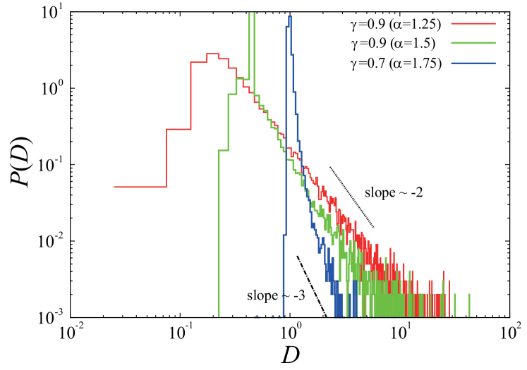
Figure 2: Histograms of the normalized diffusion coefficients $D\equiv D_{t}/\langle D_{t}\rangle$ for different $\gamma$ and $\alpha$ ($t=10^{6}$). We calculate $D_{t}$ by $\overline{\delta^{2}(\Delta;t)}/\Delta$ in numerical simulations with $\Delta=10$. The dashed line segments represent power-law distributions with exponent $-2$ and $-3$ for reference.

V.2 Equilibrium Renewal Process

In an equilibrium renewal process, i.e., $1<\alpha<2$ and $0<2\gamma<\alpha-1$, the Laplace transform ${\hat{P}_{2}}^{eq}(k,s)$ is given by

$${\hat{P}_{2}}^{eq}(k,s)=\frac{1}{s}-\frac{1-\hat{w}(s)}{\mu s}\frac{1-{\hat{\phi}}(k,0)}{1-{\hat{\phi}}(k,s)}.$$ (56)

Thus, we have the Laplace transform of $\langle Z_{t}\rangle_{eq}$ as follows:

$$\langle Z_{s}\rangle_{eq}=\left.-\frac{\partial\hat{P}^{eq}_{2}(k,s)}{\partial k}\right|_{k=0}=\frac{\left\langle l^{2}\right\rangle}{\mu s^{2}}=\left\langle x_{s}^{2}\right\rangle_{o}.$$ (57)

Averaging Eq. (29) over equilibrium ensemble, we have

$$\langle\overline{\delta^{2}(\Delta;t)}\rangle_{eq}\simeq\left\langle D_{t}\right\rangle_{eq}\Delta=\frac{\langle Z_{t}\rangle_{eq}}{t}\Delta=\frac{\left\langle l^{2}\right\rangle}{\mu}\Delta,$$ (58)

where the second moment of the first jump length is finite for $0<\gamma<\alpha-1$, otherwise the ensemble average of the TAMSD diverges. The second moment of the diffusion constant is also derived in the similar way:

$$\langle Z_{s}^{2}\rangle_{eq}=\left.\frac{\partial^{2}\hat{P}^{eq}_{2}(k,s)}{\partial k^{2}}\right|_{k=0}\simeq\frac{2\left\langle l^{2}\right\rangle^{2}}{\mu^{2}s^{3}}+\frac{2c\left\langle l^{2}\right\rangle^{2}}{\mu^{3}s^{4-\alpha}},$$ (59)

and thus we have

$$\left\langle D_{t}^{2}\right\rangle_{eq}=\frac{\left\langle l^{2}\right\rangle^{2}}{\mu^{2}}+\frac{2c\left\langle l^{2}\right\rangle^{2}}{\mu^{3}\Gamma(4-\alpha)}t^{1-\alpha},$$ (60)

for $0<\gamma<\alpha-1$. From these results, RSD is given by

$$\sigma^{2}_{\mathrm{EB}}(t)\simeq\frac{2c}{\mu}\frac{t^{1-\alpha}}{\Gamma(4-\alpha)}.$$ (61)

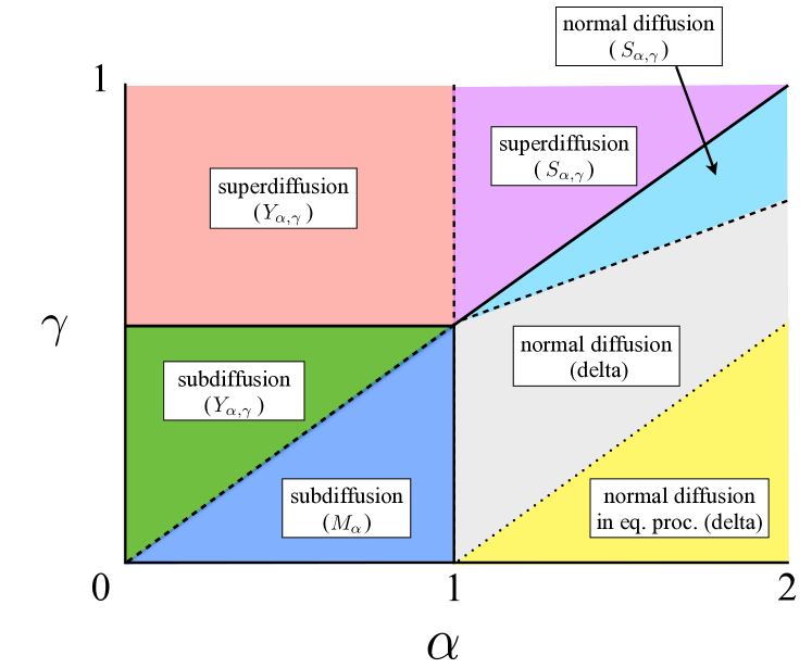
Figure 3: Phase diagram of the SEDLF in ordinary and equilibrium renewal processes. Solid lines divide the phase of the EAMSD in the ordinary renewal process. The dashed lines divide the phase of the distribution function of the TAMSD. Only below the dotted line $2\gamma<\alpha-1$, the equilibrium process exists.

VI Discussion

We have shown the phase diagram based on the power-law exponent of anomalous diffusion and the distribution of TAMSDs in SEDLF. Although SEDLF is closely related to CTRW, Lévy walk, and Lévy flight, its statistical properties on anomalous diffusion are different form them. In particular, while the visit points in SEDLF are the same as the turning points of a random walker in Lévy walk Shlesinger1987 (27), a random walker cannot move while it is trapped in SEDLF, which is completely different from Lévy walk. This discrepancy makes the scaling of TAMSD different. In fact, TAMSDs in SEDLF increase linearly with time even when the EAMSD shows superdiffusion. On the other hand, TAMSDs show superlinear scaling (superdiffusion) in Lévy walk. Because a particle is always moving and there is a power-law coupling between waiting times and moving length in turbulent diffusion and diffusion of cold atoms Shlesinger1987 (27, 30), a moving model of SEDLF can be applied to them. On the other hand, a wait and jump model (SEDLF) will be important in finance and earthquakes. In particular, SEDLF will be applied to describe dynamics of energy released in earthquake because energy is gradually accumulated and released in earthquake. Since TAMSDs can not be represented by Eq. (28) in a moving model such as Lévy walk and a moving model of SEDLF, to investigate ergodic properties of TAMSDs in a moving model of SEDLF is left for future work.

VII Conclusion

In conclusion, we have shown the phase diagram in SEDLF for a wide range of parameters, where the EAMSD shows normal diffusion, subdiffusion and superdiffusion, and the distribution of the TAMSD depends on the power-law exponent $\alpha$ of the trapping-time distribution as well as the coupling parameter $\gamma$. We consider two typical processes: ordinary renewal process and equilibrium renewal process. An equilibrium distribution for the first renewal time (the forward recurrence time) exists in renewal processes when the mean of interoccurrence time between successive renewals does not diverge. However, even when the mean does not diverge, an equilibrium distribution does not exist in the SEDLF because of divergence of the second moment of the first jump length. Therefore, we have found that the TAMSDs remain random in some parameter region even when the mean trapping time does not diverge. In particular, it is interesting to note that this distributional ergodicity is observed even when the EAMSD shows a normal diffusion, i.e., $\frac{\alpha+1}{2}<2\gamma<\alpha$ and $1<\alpha<2$. In this regime, both the mean trapping time and the second moment of jump length are finite. Therefore, this result provides a novel route to the distributional ergodicity, because so far the distributional ergodicity has been found only in systems with the divergent mean trapping time or the divergent second moment of jump length, which break down the law of large numbers.

Appendix A Derivation of $\psi_{0}(x,t)$

Here, we derive the joint PDF $\psi_{0}(x,t)$ of the first jump length $x$ and the first apparent trapping time $t$ for an equilibrium renewal process ($\alpha>1$). Let $\psi_{0,n}(x,t;t_{a})$ be the joint PDF that the first jump and the first apparent trapping time after time $t_{a}$ given that the number of jumps in $[0,t_{a}]$ is $n$. The joint PDF can be represented by

$$\psi_{0,n}(x,t;t_{a})= \frac{1}{2}\langle\delta(x-(t_{n+1}-t_{n})^{\gamma})\delta(t-(t_{n+1}-t_{a}))I(t_{n}<t_{a}<t_{n+1})\rangle$$ (62)

$$+\frac{1}{2}\langle\delta(x+(t_{n+1}-t_{n})^{\gamma})\delta(t-(t_{n+1}-t_{a}))I(t_{n}<t_{a}<t_{n+1})\rangle$$ (63)

The Fourier and double Laplace transform with respect to $x,t$ and $t_{a}$ is given by

$$\hat{\psi}_{0,n}(k,s;s_{a}) \equiv \int_{-\infty}^{\infty}dx\int_{0}^{\infty}dt\int_{0}^{\infty}dt_{a}e^{ikx}e^{-st}e^{-s_{a}t_{a}}\psi_{0,n}(x,t;t_{a})$$ (64)

$$= \left\langle\int_{t_{n}}^{t_{n+1}}dt_{a}\frac{e^{ik\tau_{n+1}^{\gamma}}+e^{-ik\tau_{n+1}^{\gamma}}}{2}e^{-s(t_{n+1}-t_{a})}e^{-s_{a}t_{a}}\right\rangle$$ (65)

$$= \frac{1}{s-s_{a}}\langle e^{-s_{a}t_{n}}\rangle\left\langle(e^{-s_{a}\tau_{n+1}}-e^{-s\tau_{n+1}})\cos(k\tau_{n+1}^{\gamma})\right\rangle$$ (66)

$$= \frac{1}{s-s_{a}}\hat{w}(s_{a})^{n}[\hat{\psi}(k,s_{a})-\hat{\psi}(k,s)].$$ (67)

Therefore, the Fourier and double Laplace transform of the joint PDF of the first jump length $x$ and the first apparent trapping time $t$ after time $t_{a}$, is given by

$$\hat{\psi}_{0}(k,s;s_{a}) = \sum_{n=0}^{\infty}\hat{\psi}_{0,n}(k,s;s_{a})$$ (68)

$$= \frac{1}{s_{a}-s}\frac{\hat{\psi}(k,s_{a})-\hat{\psi}(k,s)}{1-\hat{w}(s_{a})}.$$ (69)

Therefore, the Laplace transform of $\psi_{0}(x,t)$ is given by

$$\hat{\psi}_{0}(k,s) = \lim_{s_{a}\to 0}s_{a}\hat{\psi}_{0}(k,s;s_{a})$$ (70)

$$= \frac{\hat{\psi}(k,0)-\hat{\psi}(k,s)}{\mu s}.$$ (71)

Through the inverse Fourier-Laplace transforms of $\hat{\psi}_{0}(k,s)$, we obtain Eq. (8).

References

(1)
A. Caspi,
R. Granek, and
M. Elbaum,
Phys. Rev. Lett. 85,
5655 (2000).
(2)
I. Golding and
E. C. Cox,
Phys. Rev. Lett. 96,
098102 (2006).
(3)
A. Granéli,
C. C. Yeykal,
R. B. Robertson,
and E. C.
Greene, Proc. Natl. Acad. Sci. USA
103, 1221 (2006).
(4)
A. Weigel,
B. Simon,
M. Tamkun, and
D. Krapf,
Proc. Natl. Acad. Sci. USA 108,
6438 (2011).
(5)
J.-H. Jeon,
V. Tejedor,
S. Burov,
E. Barkai,
C. Selhuber-Unkel,
K. Berg-Sørensen,
L. Oddershede,
and R. Metzler,
Phys. Rev. Lett. 106,
048103 (2011).
(6)
S. C. Weber,
A. J. Spakowitz,
and J. A.
Theriot, Proc. Natl. Acad. Sci. USA
109, 7338 (2012).
(7)
S. A. Tabei,
S. Burov,
H. Y. Kim,
A. Kuznetsov,
T. Huynh,
J. Jureller,
L. H. Philipson,
A. R. Dinner,
and N. F.
Scherer, Proc. Natl. Acad. Sci. USA
110, 4911 (2013).
(8)
M. Magdziarz,
A. Weron,
K. Burnecki, and
J. Klafter,
Phys. Rev. Lett. 103,
180602 (2009).
(9)
V. Tejedor,
O. Bénichou,
R. Voituriez,
R. Jungmann,
F. Simmel,
C. Selhuber-Unkel,
L. B. Oddershede,
and R. Metzler,
Biophysical J. 98,
1364 (2010).
(10)
E. Kepten,
I. Bronshtein,
and Y. Garini,
Phys. Rev. E 83,
041919 (2011).
(11)
M. Magdziarz and
A. Weron,
Phys. Rev. E 84,
051138 (2011).
(12)
Y. Meroz,
I. M. Sokolov,
and J. Klafter,
Phys. Rev. Lett. 110,
090601 (2013).
(13)
A. Lubelski,
I. M. Sokolov,
and J. Klafter,
Phys. Rev. Lett. 100,
250602 (2008).
(14)
Y. He,
S. Burov,
R. Metzler, and
E. Barkai,
Phys. Rev. Lett. 101,
058101 (2008).
(15)
T. Miyaguchi and
T. Akimoto,
Phys. Rev. E 83,
062101 (2011).
(16)
T. Miyaguchi and
T. Akimoto,
Phys. Rev. E 83,
031926 (2011).
(17)
T. Akimoto and
T. Miyaguchi,
Phys. Rev. E 82,
030102(R) (2010).
(18)
J. Bouchaud and
A. Georges,
Phys. Rep. 195,
127 (1990).
(19)
T. Akimoto and
Y. Aizawa,
Chaos 20,
033110 (2011).
(20)
J. Aaronson,
An Introduction to Infinite Ergodic Theory
(American Mathematical Society,
Providence, 1997).
(21)
X. Brokmann,
J.-P. Hermier,
G. Messin,
P. Desbiolles,
J.-P. Bouchaud,
and M. Dahan,
Phys. Rev. Lett. 90,
120601 (2003).
(22)
F. D. Stefani,
J. P. Hoogenboom,
and E. Barkai,
Phys. Today 62,
34 (2009).
(23)
T. Akimoto and
T. Miyaguchi,
Phys. Rev. E 87,
062134 (2013).
(24)
J. Klafter,
A. Blumen, and
M. F. Shlesinger,
Phys. Rev. A 35,
3081 (1987).
(25)
M. Magdziarz,
W. Szczotka, and
P. Żebrowski,
J. Stat. Phys. 147,
74 (2012).
(26)
J. Liu and
J.-D. Bao,
Physica A 392,
612 (2013).
(27)
M. F. Shlesinger,
B. J. West, and
J. Klafter,
Phys. Rev. Lett. 58,
1100 (1987).
(28)
T. Akimoto,
Phys. Rev. Lett. 108,
164101 (2012).
(29)
D. Froemberg and
E. Barkai,
Phys. Rev. E 87,
030104 (2013a).
(30)
E. Barkai,
E. Aghion, and
D. Kessler,
Phys. Rev. X 4,
021036 (2014).
(31)
M. M. Meerschaert
and E. Scalas,
Physica A 370,
114 (2006).
(32)
A. Corral,
Phys. Rev. Lett. 97,
178501 (2006).
(33)
E. Lippiello,
C. Godano, and
L. de Arcangelis,
Europhys. Lett. 102,
59002 (2013).
(34)
D. R. Cox,
Renewal theory (Methuen,
London, 1962).
(35)
M. Shlesinger,
J. Klafter, and
Y. Wong, J.
Stat. Phys. 27, 499
(1982).
(36)
E. Barkai,
Phys. Rev. Lett. 90,
104101 (2003).
(37)
J. H. P. Schulz,
E. Barkai, and
R. Metzler,
Phys. Rev. Lett. 110,
020602 (2013).
(38)
T. Akimoto,
S. Shinkai, and
Y. Aizawa,
arxiv:1310.4055.
(39)
G. Zumofen and
J. Klafter,
Physica D 69,
436 (1993).
(40)
A. Godec and
R. Metzler,
Phys. Rev. Lett. 110,
020603 (2013).
(41)
D. Froemberg and
E. Barkai,
Eur. Phys. J. B 86,
331 (2013b).
(42)
T. Akimoto and
Y. Aizawa, J
Korean Phys. Soc. 50, 254
(2007).
(43)
T. Miyaguchi and
T. Akimoto,
Phys. Rev. E 87,
032130 (2013).
(44)
T. Akimoto,
E. Yamamoto,
K. Yasuoka,
Y. Hirano, and
M. Yasui,
Phys. Rev. Lett. 107,
178103 (2011).
(45)
T. Uneyama,
T. Akimoto, and
T. Miyaguchi,
J. Chem. Phys. 137,
114903 (2012).