Abstract: We give an algorithm which for an input planar graph $G$ of $n$ vertices and integer $k$, in $\min\{O(n\log^{3}n),O(nk^{2})\}$ time either constructs a branch-decomposition of $G$ with width at most $(2+\delta)k$, $\delta>0$ is a constant, or a $(k+1)\times\lceil{\frac{k+1}{2}}\rceil$ cylinder minor of $G$ implying ${\mathop{\rm bw}}(G)>k$, ${\mathop{\rm bw}}(G)$ is the branchwidth of $G$. This is the first $\tilde{O}(n)$ time constant-factor approximation for branchwidth/treewidth and largest grid/cylinder minors of planar graphs and improves the previous $\min\{O(n^{1+\epsilon}),O(nk^{2})\}$ ($\epsilon>0$ is a constant) time constant-factor approximations. For a planar graph $G$ and $k={\mathop{\rm bw}}(G)$, a branch-decomposition of width at most $(2+\delta)k$ and a $g\times\frac{g}{2}$ cylinder/grid minor with $g=\frac{k}{\beta}$, $\beta>2$ is constant, can be computed by our algorithm in $\min\{O(n\log^{3}n\log k),O(nk^{2}\log k)\}$ time.

Key words: Branch-/tree-decompositions, grid minor, planar graphs, approximation algorithm.

1 Introduction

The notions of branchwidth and branch-decomposition introduced by Robertson and Seymour [31] in relation to the notions of treewidth and tree-decomposition have important algorithmic applications. The branchwidth ${\mathop{\rm bw}}(G)$ and the treewidth ${\mathop{\rm tw}}(G)$ of graph $G$ are linearly related: $\max\{{\mathop{\rm bw}}(G),2\}\leq{\mathop{\rm tw}}(G)+1\leq\max\{\lfloor{\frac{3}{2}{\mathop{\rm bw}}(G)}\rfloor,2\}$ for every $G$ with more than one edge, and there are simple translations between branch-decompositions and tree-decompositions that meet the linear relations [31]. A graph $G$ of small branchwidth (treewidth) admits efficient algorithms for many NP-hard problems [2, 7]. These algorithms first compute a branch-/tree-decomposition of $G$ and then apply a dynamic programming algorithm based on the decomposition to solve the problem. The dynamic programming step usually runs in polynomial time in the size of $G$ and exponential time in the width of the branch-/tree-decomposition computed.

Deciding the branchwidth/treewidth and computing a branch-/tree-decomposition of minimum width have been extensively studied. For an arbitrary graph $G$ of $n$ vertices, the following results have been known: Given an integer $k$, it is NP-complete to decide whether ${\mathop{\rm bw}}(G)\leq k$ [34] (${\mathop{\rm tw}}(G)\leq k$ [1]). If ${\mathop{\rm bw}}(G)$ (${\mathop{\rm tw}}(G)$) is upper-bounded by a constant then both the decision problem and the optimal decomposition problem can be solved in $O(n)$ time [10, 8]. However, the linear time algorithms are mainly of theoretical importance because the constant behind the Big-Oh is huge. The best known polynomial time approximation factor is $O(\sqrt{{\mathop{\rm bw}}(G)})$ for branchwidth and $O(\sqrt{\log{\mathop{\rm tw}}(G)})$ for treewidth [15]. The best known exponential time approximation factors are as follows: an algorithm giving a branch-decomposition of width at most $3{\mathop{\rm bw}}(G)$ in $2^{O({\mathop{\rm bw}}(G))}n^{2}$ time [32]; an algorithm giving a tree-decomposition of width at most $3{\mathop{\rm tw}}(G)+4$ in $2^{O({\mathop{\rm bw}}(G))}n\log n$ time [6]; and an algorithm giving a tree-decomposition of width at most $5{\mathop{\rm tw}}(G)+4$ in $2^{O({\mathop{\rm tw}}(G))}n$ time [6]. By the linear relation between the branchwidth and treewidth, the algorithms for tree-decompositions are also algorithms of same approximation factors for branch-decompositions, while from a branchwidth approximation $\alpha$, a treewidth approximation $1.5\alpha$ can be obtained.

Better results have been known for planar graphs $G$. Seymour and Thomas show that whether ${\mathop{\rm bw}}(G)\leq k$ can be decided in $O(n^{2})$ time and an optimal branch-decomposition of $G$ can be computed in $O(n^{4})$ time [34]. Gu and Tamaki improve the $O(n^{4})$ time for the optimal branch-decomposition to $O(n^{3})$ [18]. By the linear relation between the branchwidth and treewidth, the above results imply polynomial time $1.5$-approximation algorithms for the treewidth and optimal tree-decomposition of planar graphs. It is open whether deciding ${\mathop{\rm tw}}(G)\leq k$ is NP-complete or polynomial time solvable for planar graphs $G$.

Fast algorithms for computing small width branch-/tree-decompositions of planar graphs have received much attention as well. Tamaki gives an $O(n)$ time heuristic algorithm for branch-decomposition [36]. Gu and Tamaki give an algorithm which for an input planar graph $G$ of $n$ vertices and integer $k$, either constructs a branch-decomposition of $G$ with width at most $(c+1+\delta)k$ or outputs ${\mathop{\rm bw}}(G)>k$ in $O(n^{1+\frac{1}{c}})$ time, where $c$ is any fixed positive integer and $\delta>0$ is any constant [19]. By this algorithm and a binary search, a branch-decomposition of width at most $(c+1+\delta)k$ can be computed in $O(n^{1+\frac{1}{c}}\log k)$ time, $k={\mathop{\rm bw}}(G)$. Kammer and Tholey give an algorithm which for input $G$ and $k$, either constructs a tree-decomposition of $G$ with width $O(k)$ or outputs ${\mathop{\rm tw}}(G)>k$ in $O(nk^{3})$ time [26, 27]. The time complexity of the algorithm is improved to $O(nk^{2})$ recently [28]. This implies that a tree-decomposition of width $O(k)$ can be computed in $O(nk^{2}\log k)$ time, $k={\mathop{\rm tw}}(G)$. Computational study on branch-decomposition can be found in [3, 4, 5, 23, 24, 35, 36]. Fast constant-factor approximation algorithms for branch-/tree-decompositions of planar graphs have important applications such as that in shortest distance oracles in planar graphs [29].

Grid minor of graphs is another notion in graph minor theory [33]. A $k\times k$ grid is a Cartesian product of two paths, each on $k$ vertices. For a graph $G$, let ${\mathop{\rm gm}}(G)$ be the largest integer $k$ such that $G$ has a $k\times k$ grid as a minor. Computing a large grid minor of a graph is important in algorithmic graph minor theory and bidimensionality theory [13, 14, 33]. It is shown in [33] that ${\mathop{\rm gm}}(G)\leq{\mathop{\rm bw}}(G)\leq 4{\mathop{\rm gm}}(G)$ for planar graphs. Gu and Tamaki improve the linear bound ${\mathop{\rm bw}}(G)\leq 4{\mathop{\rm gm}}(G)$ to ${\mathop{\rm bw}}(G)\leq 3{\mathop{\rm gm}}(G)$ and show that for any $a<2$, ${\mathop{\rm bw}}(G)\leq a{\mathop{\rm gm}}(G)$ does not hold for planar graphs [20]. Other studies on grid minor size and branchwidth/treewidth of planar graphs can be found in [9, 17]. The upper bound ${\mathop{\rm bw}}(G)\leq 3{\mathop{\rm gm}}(G)$ is a consequence of a result on cylinder minors. A $k\times h$ cylinder is a Cartesian product of a cycle on $k$ vertices and a path on $h$ vertices. For a graph $G$, let ${\mathop{\rm cm}}(G)$ be the largest integer $k$ such that $G$ has a $k\times\lceil{\frac{k}{2}}\rceil$ cylinder as a minor. It is shown in [20] that ${\mathop{\rm cm}}(G)\leq{\mathop{\rm bw}}(G)\leq 2{\mathop{\rm cm}}(G)$ for planar graphs. The $O(n^{1+\frac{1}{c}})$ time algorithm in [19] actually constructs a branch-decomposition of $G$ with width at most $(c+1+\delta)k$ or a $(k+1)\times\lceil{\frac{k+1}{2}}\rceil$ cylinder minor.

We propose an $\tilde{O}(n)$ time constant-factor approximation algorithm for branch-/tree-decompositions of planar graphs. Our main result is as follows.

Theorem 1

There is an algorithm which given a planar graph $G$ of $n$ vertices and an integer $k$, in $\min\{O(n\log^{3}n),O(nk^{2})\}$ time either constructs a branch-decomposition of $G$ with width at most $(2+\delta)k$, $\delta>0$ is a constant, or a $(k+1)\times\lceil{\frac{k+1}{2}}\rceil$ cylinder minor of $G$.

Since a $(k+1)\times\lceil{\frac{k+1}{2}}\rceil$ cylinder has branchwidth at least $k+1$ [20], a cylinder minor given in Theorem 1 implies ${\mathop{\rm bw}}(G)>k$.

By the linear relation between the branchwidth and treewidth, Theorem 1 implies an algorithm which for an input planar graph $G$ and integer $k$, in $\min\{O(nk+n\log^{3}n),O(nk^{2})\}$ time constructs a tree-decomposition of $G$ with width at most $(3+\delta)k$ or outputs ${\mathop{\rm tw}}(G)>k$. For a planar graph $G$ and $k={\mathop{\rm bw}}(G)$, by Theorem 1 and a binary search, a branch-decomposition of $G$ with width at most $(2+\delta)k$ can be computed in $\min\{O(n\log^{3}n\log k),O(nk^{2}\log k)\}$ time. This improves the previous result of a branch-decomposition of width at most $(c+1+\delta)k$ in $O(n^{1+\frac{1}{c}}\log k)$ time [19]. Similarly, for a planar graph $G$ and $k={\mathop{\rm tw}}(G)$, a tree-decomposition of width at most $(3+\delta)k$ can be computed in $\min\{O(nk+n\log^{3}n\log k),O(nk^{2}\log k)\}$ time. Kammer and Tholey give an algorithm which computes a tree-decomposition of $G$ with width at most $48k+13$ in $O(nk^{3}\log k)$ time or with width at most $(9+\delta)k+9$ in $O(n\min\{\frac{1}{\delta},k\}k^{3}\log k)$ time ($0<\delta<1$) [26, 27]. Recently, Kammer and Tholey give an algorithm for computing weighted treewidth for vertex weighted planar graphs [28]. Applying this algorithm to planar graph $G$, a tree-decomposition of $G$ with width at most $(15+\delta)k+O(1)$ can be computed in $O(nk^{2}\log k)$ time. This improves the result of [26, 27]. Our $O(nk^{2}\log k)$ time algorithm is an independent improvement over the result of [26, 27] and has a better approximation ratio than that of [28]. Our algorithm can also be used to compute a $g\times\lceil{\frac{g}{2}}\rceil$ cylinder (grid) minor with $g=\frac{{\mathop{\rm bw}}(G)}{\beta}$, $\beta>2$ is a constant, and a $g\times g$ cylinder (grid) minor with $g=\frac{{\mathop{\rm bw}}(G)}{\beta}$, $\beta>3$ is a constant, of $G$ in $\min\{O(n\log^{3}n\log k),O(nk^{2}\log k)\}$ time. This improves the previous results of $g\times\lceil{\frac{g}{2}}\rceil$ with $g\geq\frac{{\mathop{\rm bw}}(G)}{\beta}$, $\beta>(c+1)$, and $g\times g$ with $g\geq\frac{{\mathop{\rm bw}}(G)}{\beta}$, $\beta>(2c+1)$, in $O(n^{1+\frac{1}{c}}\log k)$ time. As an application, our algorithm removes a bottleneck in the work of [29] for computing a shortest path oracle and reduces its preprocessing time in Theorem 6.1 from $O(n^{1+\frac{1}{c}}\log k\log n+S\log^{2}n)$ to $O(\min\{O(n\log^{4}n\log k),O(nk^{2}\log n\log k)\}+S\log^{2}n)$.

Our algorithm for Theorem 1 uses the approach in the previous work of [19] described below. Given a planar graph $G$ and integer $k$, let ${\cal Z}$ be the set of biconnected components of $G$ with a normal distance (a definition is given in the next section) $h=ak$, $a>0$ is a constant, from a selected edge $e_{0}$ of $G$. For each $Z\in{\cal Z}$, a minimum vertex cut set $\partial(A_{Z})$ which partitions $E(G)$ into edge subsets $A_{Z}$ and $\overline{A}_{Z}=E(G)\setminus A_{Z}$ is computed such that $Z\subseteq A_{Z}$ and $e_{0}\in\overline{A}_{Z}$, that is, $\partial(A_{Z})$ separates $Z$ and $e_{0}$. If $|\partial(A_{Z})|>k$ for some $Z\in{\cal Z}$ then ${\mathop{\rm bw}}(G)>k$ is concluded. Otherwise, a branch-decomposition of graph $H$ obtained from $G$ by removing all $A_{Z}$ is constructed. For each subgraph $G[A_{Z}]$ induced by $A_{Z}$, a branch-decomposition is constructed or ${\mathop{\rm bw}}(G[A_{Z}])>k$ is concluded recursively. Finally, a branch-decomposition of $G$ with width $O(k)$ is constructed from the branch-decomposition of $H$ and those of $G[A_{Z}]$ or ${\mathop{\rm bw}}(G)>k$ is concluded.

The algorithm in [19] computes a minimum vertex cut set $\partial(A_{Z})$ for every $Z\in{\cal Z}$ in all recursive steps in $O(n^{1+\frac{1}{c}})$ time. Our main idea for proving Theorem 1 is to find a minimum vertex cut set $\partial(A_{Z})$ for every $Z\in{\cal Z}$ more efficiently based on recent results for computing minimum face separating cycles and vertex cut sets in planar graphs. Borradaile et al. give an algorithm which in $O(n\log^{4}n)$ time computes an oracle for the all pairs minimum face separating cycle problem in a planar graph $G$ [12]. The time for computing the oracle is further improved to $O(n\log^{3}n)$ [11]. For any pair of faces $f$ and $g$ in $G$, the oracle in $O(|C|)$ time returns a minimum $(f,g)$-separating cycle $C$ ($C$ cuts the sphere on which $G$ is embedded into two regions, one contains $f$ and the other contains $g$). By this result, we show that a minimum vertex cut set $\partial(A_{Z})$ for every $Z\in{\cal Z}$ in all recursive steps can be computed in $O(n\log^{3}n)$ time and get the next result.

Theorem 2

There is an algorithm which given a planar graph $G$ of $n$ vertices and an integer $k$, in $O(n\log^{3}n)$ time either constructs a branch-decomposition of $G$ with width at most $(2+\delta)k$ or a $(k+1)\times\lceil{\frac{k+1}{2}}\rceil$ cylinder minor of $G$, where $\delta>0$ is a constant.

For an input $G$ and integer $k$, Kammer and Tholey give an algorithm which in $O(nk^{3})$ time constructs a tree-decomposition of width $O(k)$ or outputs ${\mathop{\rm tw}}(G)>k$ as follows [26, 27]: Convert $G$ into an almost triangulated planar graph $\hat{G}$. Use crest separators to decompose $\hat{G}$ into pieces (subgraphs), each piece contains one component (called crest with a normal distance $k$ from a selected set of edges called coast). For each crest compute a vertex cut set of size at most $3k-1$ to separate the crest from the coast. If such a vertex cut set can not be found for some crest then the algorithm concludes ${\mathop{\rm tw}}(\hat{G})>k$. Otherwise, the algorithm computes a tree-decomposition for the graph $\hat{H}$ obtained by removing all crests from $\hat{G}$ and works on each crest recursively. Finally, the algorithm constructs a tree-decomposition of $\hat{G}$ from the tree-decomposition of $\hat{H}$ and those of crests.

To get an $O(nk^{2})$ time algorithm for Theorem 1, we apply the ideas of triangulating $G$ and crest separators in [26, 27] to decompose $\hat{G}$ into pieces, each piece having one component (crest) $Z\in{\cal Z}$. Instead of finding a vertex cut set of size at most $3k-1$ for each crest, we apply the minimum face separating cycle to find a minimum vertex cut set $\partial(A_{Z})$ in each piece. We show that either a vertex cut set $\partial(A_{Z})$ with $|\partial(A_{Z})|\leq k$ for every $Z\in{\cal Z}$ in all recursive steps or a $(k+1)\times\lceil{\frac{k+1}{2}}\rceil$ cylinder minor can be computed in $O(nk^{2})$ time and get the result below.

Theorem 3

There is an algorithm which given a planar graph $G$ of $n$ vertices and an integer $k$, in $O(nk^{2})$ time either constructs a branch-decomposition of $G$ with width at most $(2+\delta)k$ or a $(k+1)\times\lceil{\frac{k+1}{2}}\rceil$ cylinder minor of $G$, where $\delta>0$ is a constant.

Theorem 1 follows from Theorems 2 and 3.

The next section gives the preliminaries of the paper. We prove Theorems 2 and 3 in Sections 3 and 4, respectively. The final section concludes the paper.

2 Preliminaries

It is convenient to view a vertex cut set $\partial(A_{Z})$ in a graph as an edge in a hypergraph in some cases. A hypergraph $G$ consists of a set $V(G)$ of vertices and a set $E(G)$ of edges, each edge is a subset of $V(G)$ with at least two elements. A hypergraph $G$ is a graph if for every $e\in E(G)$, $e$ has two elements. For a subset $A\subseteq E(G)$, we denote $\cup_{e\in A}e$ by $V(A)$ and denote $E(G)\setminus A$ by $\overline{A}$. For $A\subseteq E(G)$, the pair $(A,\overline{A})$ is a separation of $G$ and we denote by $\partial(A)$ the vertex set $V(A)\cap V(\overline{A})$. The order of separation $(A,\overline{A})$ is $|\partial(A)|$. A hypergraph $H$ is a subgraph of $G$ if $V(H)\subseteq V(G)$ and $E(H)\subseteq E(G)$. For $A\subseteq E(G)$ and $W\subseteq V(G)$, we denote by $G[A]$ and $G[W]$ the subgraphs of $G$ induced by $A$ and $W$, respectively. For a subgraph $H$ of $G$, we denote $G[E(G)\setminus E(H)]$ by $G\setminus H$.

A walk in graph $G$ is a sequence of edges $e_{1},e_{2},...,e_{k}$, where $e_{i}=\{v_{i-1},v_{i}\}$. We call $v_{0}$ and $v_{k}$ the end vertices and other vertices the internal vertices of the walk. A walk is a path if all vertices in the walk are distinct. A walk is a cycle if it has at least three vertices, $v_{0}=v_{k}$ and $v_{1},...,v_{k}$ are distinct. A graph is weighted if each edge of the graph is assigned a weight. Unless otherwise stated, a graph is unweighted. The length of a walk in a graph is the number of edges in the walk. The length of a walk in a weighted graph is the sum of the weights of the edges in the walk.

The notions of branchwidth and branch-decomposition are introduced by Robertson and Seymour [31]. A branch-decomposition of hypergraph $G$ is a pair $(\phi,T)$ where $T$ is a ternary tree and $\phi$ is a bijection from the set of leaves of $T$ to $E(G)$. We refer the edges of $T$ as links and the vertices of $T$ as nodes. Consider a link $e$ of $T$ and let $L_{1}$ and $L_{2}$ denote the sets of leaves of $T$ in the two respective subtrees of $T$ obtained by removing $e$. We say that the separation $(\phi(L_{1}),\phi(L_{2}))$ is induced by this link $e$ of $T$. We define the width of the branch-decomposition $(\phi,T)$ to be the largest order of the separations induced by links of $T$. The branchwidth of $G$, denoted by ${\mathop{\rm bw}}(G)$, is the minimum width of all branch-decompositions of $G$. In the rest of this paper, we identify a branch-decomposition $(\phi,T)$ with the tree $T$, leaving the bijection implicit and regarding each leaf of $T$ as a edge of $G$.

Let $\Sigma$ be a sphere. For an open segment $s$ homeomorphic to $\{x|0<x<1\}$ in $\Sigma$, we denote by ${\mathop{\rm cl}}(s)$ the closure of $s$. A planar embedding of a graph $G$ is a mapping $\rho:V(G)\cup E(G)\to\Sigma\cup 2^{\Sigma}$ such that

• for $u\in V(G)$, $\rho(u)$ is a point of $\Sigma$, and for distinct $u,v\in V(G)$, $\rho(u)\neq\rho(v)$;

• for each edge $e=\{u,v\}\in E(G)$, $\rho(e)$ is an open segment in $\Sigma$ with $\rho(u)$ and $\rho(v)$ the two end points in ${\mathop{\rm cl}}(\rho(e))\setminus\rho(e)$; and

• for distinct $e_{1},e_{2}\in E(G)$, ${\mathop{\rm cl}}(\rho(e_{1}))\cap{\mathop{\rm cl}}(\rho(e_{2}))=\{\rho(u)|u\in e_{1}\cap e_{2}\}$.

A graph $G$ is planar if it has a planar embedding $\rho$, and $(G,\rho)$ is called a plane graph. We may simply use $G$ to denote the plane graph $(G,\rho)$, leaving the embedding $\rho$ implicit. For a plane graph $G$, each connected component of $\Sigma\setminus(\cup_{e\in E(G)}{\mathop{\rm cl}}(\rho(e)))$ is a face of $G$. We denote by $V(f)$ and $E(f)$ the set of vertices and the set of edges incident to face $f$, respectively. We say that face $f$ is bounded by the edges of $E(f)$.

A graph $G$ of at least three vertices is biconnected if for any pairwise distinct vertices $u,v,w\in V(G)$, there is a path of $G$ between $u$ and $v$ that does not contain $w$. Graph $G$ of a single vertex or a single edge is (degenerated) biconnected. A biconnected component of $G$ is a maximum biconnected subgraph of $G$. It suffices to prove Theorems 2 and 3 for a biconnected $G$ because if $G$ is not biconnected, the problems of finding branch-decompositions and cylinder minors of $G$ can be solved individually for each biconnected component.

For a plane graph $G$, a curve $\mu$ on $\Sigma$ is normal if $\mu$ does not intersect any edge of $G$. The length of a normal curve $\mu$ is the number of connected components of $\mu\setminus\bigcup_{v\in V(G)}\{\rho(v)\}$. For vertices $u,v\in V(G)$, the normal distance ${\mathop{\rm nd}}_{G}(u,v)$ is defined as the shortest length of a normal curve between $\rho(u)$ and $\rho(v)$. The normal distance between two vertex-subsets $U,W\subseteq V(G)$ is defined as ${\mathop{\rm nd}}_{G}(U,W)=\min_{u\in U,v\in W}{\mathop{\rm nd}}_{G}(u,v)$. We also use ${\mathop{\rm nd}}_{G}(U,v)$ for ${\mathop{\rm nd}}_{G}(U,\{v\})$ and ${\mathop{\rm nd}}_{G}(u,W)$ for ${\mathop{\rm nd}}_{G}(\{u\},W)$.

A noose of $G$ is a closed normal curve on $\Sigma$ that does not intersect with itself. A noose $\nu$ of $G$ separates $\Sigma$ into two open regions $R_{1}$ and $R_{2}$ and induces a separation $(A,\overline{A})$ of $G$ with $A=\{e\in E(G)\mid\rho(e)\subseteq R_{1}\}$ and $\overline{A}=\{e\in E(G)\mid\rho(e)\subseteq R_{2}\}$. We also say $\nu$ induces edge subset $A$ ($\overline{A}$). A separation (resp. an edge subset) of $G$ is called noose-induced if there is a noose which induces the separation (resp. edge subset). A noose $\nu$ separates two edge subsets $A_{1}$ and $A_{2}$ if $\nu$ induces a separation $(A,\overline{A})$ with $A_{1}\subseteq A$ and $A_{2}\subseteq\overline{A}$. We also say that the noose induced subset $A$ separates $A_{1}$ and $A_{2}$.

For plane graph $G$ and a noose $\nu$ induced $A\subseteq E(G)$, we denote by $G|A$ the plane hypergraph obtained by replacing all edges of $A$ with edge $\partial(A)$ (i.e., $V(G|A)=(V(G)\setminus V(A))\cup\partial(A)$ and $E(G|A)=(E(G)\setminus A)\cup\{\partial(A)\}$). An embedding of $G|A$ can be obtained from $G$ with $\rho(\partial(A))$ an open disk (homeomorphic to $\{(x,y)|x^{2}+y^{2}<1\}$) which is the open region separated by $\nu$ and contains $A$. For a collection ${\mathcal{A}}=\{A_{1},..,A_{r}\}$ of mutually disjoint noose induced edge-subsets of $G$, $(..(G|A_{1})|..)|A_{r}$ is denoted by $G|{\mathcal{A}}$.

3 $O(n\log^{3}n)$ time algorithm

We give an algorithm to prove Theorem 2. Our algorithm follows the approach of the work in [19]. Let $G$ be a plane graph (hypergraph) of $n$ vertices, $e_{0}$ be an arbitrary edge of $G$ and $k,h>0$ be integers. We first try to separate $e_{0}$ and the subgraph of $G$ induced by the vertices with the normal distance at least $h$ from $e_{0}$. Since the subgraph may not be biconnected, let ${\cal Z}$ be the set of biconnected components of $G$ such that for each $Z\in{\cal Z}$, ${\mathop{\rm nd}}_{G}(e_{0},V(Z))=h$. For each $Z\in{\cal Z}$, our algorithm computes a minimum noose induced subset $A_{Z}$ separating $Z$ and $e_{0}$. If for some $Z\in{\cal Z}$, $|\partial(A_{Z})|>k$ then the algorithm constructs a $(k+1)\times h$ cylinder minor of $G$ in $O(n)$ time by Lemma 1 proved in [19]. Otherwise, a set ${\mathcal{A}}$ of noose induced subsets with the following properties is computed: (1) for every $A_{Z}\in{\mathcal{A}}$, $|\partial(A_{Z})|\leq k$, (2) for every $Z\in{\cal Z}$, there is an $A_{Z}\in{\mathcal{A}}$ which separates $Z$ and $e_{0}$ and (3) for distinct $A_{Z},A_{Z^{\prime}}\in{\mathcal{A}}$, $A_{Z}\cap A_{Z}^{\prime}=\emptyset$. Such an ${\mathcal{A}}$ is called a good-separator for ${\cal Z}$ and $e_{0}$.

Lemma 1

[19] Given a plane graph $G$ and integers $k,h>0$, let $A_{1}$ and $A_{2}$ be edge subsets of $G$ satisfying the following conditions: (1) each of separations $(A_{1},\overline{A_{1}})$ and $(A_{2},\overline{A_{2}})$ is noose-induced; (2) $G[A_{2}]$ is biconnected; (3) ${\mathop{\rm nd}}_{G}(V(\overline{A_{1}}),V(A_{2}))\geq h$; and (4) every noose of $G$ that separates $\overline{A_{1}}$ and $A_{2}$ has length $>k$. Then $G$ has a $(k+1)\times h$ cylinder minor and given $(G|\overline{A_{1}})|A_{2}$, such a minor can be constructed in $O(|V(A_{1}\cap\overline{A_{2}})|)$ time.

Given a good-separator ${\mathcal{A}}$ for ${\cal Z}$ and $e_{0}$, our algorithm constructs a branch-decomposition of plane hypergraph $G|{\mathcal{A}}$ with width at most $k+2h$ by Lemma 2 shown in [20, 36]. For each $A_{Z}\in{\mathcal{A}}$, the algorithm computes a cylinder minor or a branch-decomposition for the plane hypergraph $G|\overline{A}_{Z}$ recursively. If a branch-decomposition of $G|\overline{A}_{Z}$ is found for every $A_{Z}\in{\mathcal{A}}$, the algorithm constructs a branch-decomposition of $G$ with width at most $k+2h$ from the branch-decomposition of $G|{\mathcal{A}}$ and those of $G|\overline{A}_{Z}$ by Lemma 3 which is straightforward from the definitions of branch-decompositions.

Lemma 2

[20, 36] Let $k>0$ and $h>0$ be integers. Let $G$ be a plane hypergraph with each edge of $G$ incident to at most $k$ vertices. If there is an edge $e_{0}$ such that for any vertex $v$ of $G$, ${\mathop{\rm nd}}_{G}(e_{0},v)\leq h$ then given $e_{0}$, a branch-decomposition of $G$ with width at most $k+2h$ can be constructed in $O(|V(G)|+|E(G)|)$ time.

The upper bound $k+2h$ is shown in Theorem 3.1 in [20]. The normal distance in [20] between a pair of vertices is twice of the normal distance in this paper between the same pair of vertices. Tamaki gives a linear time algorithm to construct a branch-decomposition of width at most $k+2h$ [36].

The following lemma is straightforward from the definition of branch-decompositions and allows us to bound the width of the branch-decomposition of the whole graph.

Lemma 3

Given a plane hypergraph $G$ and a noose-induced separation $(A,\overline{A})$ of $G$, let $T_{A}$ and $T_{\overline{A}}$ be branch-decompositions of $G|\overline{A}$ and $G|A$ respectively. Let $T_{A}+T_{\overline{A}}$ to be the tree obtained from $T_{A}$ and $T_{\overline{A}}$ by joining the link incident to the leaf $\partial(A)$ in $T_{A}$ and the link incident to the leaf $\partial(A)$ in $T_{\overline{A}}$ into one link and removing the leaves $\partial(A)$. Then $T_{A}+T_{\overline{A}}$ is a branch-decomposition of $G$ with width $\max\{|\partial(A)|,k_{A},k_{\overline{A}}\}$ where $k_{A}$ is the width of $T_{A}$ and $k_{\overline{A}}$ is the width of $T_{\overline{A}}$.

To make a concrete progress in each recursive step, the following technique in [19] is used to compute ${\mathcal{A}}$. For a plane hypergraph $G$, a vertex subset $e_{0}$ of $G$ and an integer $d\geq 0$, let

$${\mathop{\rm reach}}_{G}(e_{0},d)=\bigcup\{v\in V(G)|{\mathop{\rm nd}}_{G}(e_{0},v)\leq d\}$$

denote the set of vertices of $G$ with the normal distance at most $d$ from set $e_{0}$. Let $\alpha>0$ be an arbitrary constant. For integer $k\geq 2$, let $d_{1}=\lceil{\frac{\alpha k}{2}}\rceil$ and $d_{2}=d_{1}+\lceil{\frac{k+1}{2}}\rceil$. The layer tree ${\mathop{\rm LT}}(G,e_{0})$ is defined as follows:

1. the root of the tree is $G$;

2. each biconnected component $X$ of $G[V(G)\setminus{\mathop{\rm reach}}_{G}(e_{0},d_{1}-1)]$ is a node in level 1 of the tree and is a child of the root; and

3. each biconnected component $Z$ of $G[V(G)\setminus{\mathop{\rm reach}}_{G}(e_{0},d_{2}-1)]$ is a node in level 2 of the tree and is a child of the biconnected component $X$ in level 1 that contains $Z$.

For $h=d_{2}$, ${\cal Z}$ is the set of leaf nodes of ${\mathop{\rm LT}}(G,e_{0})$ in level 2. For a node $X$ of ${\mathop{\rm LT}}(G,e_{0})$ in level 1 that is not a leaf, let ${\cal Z}_{X}$ be the set of child nodes of $X$. It is shown in [19] (in the proofs of Lemma 4.1) that for any $Z\in{\cal Z}_{X}$, if a minimum noose in the plane hypergraph $(G|\overline{X})|{\cal Z}_{X}$ separating $\{\partial(Z)\}$ and $\{\partial(\overline{X})\}$ has length $>k$ then $G$ has a $(k+1)\times\lceil{\frac{k+1}{2}}\rceil$ cylinder minor. From this, a good-separator ${\mathcal{A}}_{X}$ for ${\cal Z}_{X}$ and $\overline{X}$ can be computed in hypergraph $(G|\overline{X})|{\cal Z}_{X}$, and the union of ${\mathcal{A}}_{X}$ for every $X$ gives a good-separator ${\mathcal{A}}$ for ${\cal Z}$ and $e_{0}$.

Notice that if $Z$ is a single vertex then $Z$ will not be involved any further recursive step; and if $Z$ is a single edge then there is a noose of length $2\leq k$ separating $\{\partial(Z)\}$ and $\{\partial(\overline{X})\}$, and it is trivial to compute the branch-decomposition of $Z$. So we assume without loss of generality that each $Z\in{\cal Z}_{X}$ has at least three vertices.

To compute ${\mathcal{A}}_{X}$, we convert $(G|\overline{X})|{\cal Z}_{X}$ to a weighted plane graph and compute a minimum noose induced subset $A_{Z}$ separating $Z\in{\cal Z}_{X}$ and $\overline{X}$ by finding a minimum face separating cycle in the weighted plane graph. We use the algorithm by Borradaile et al. [11] to compute the face separating cycles.

For each edge $\partial(Z)$ in $(G|\overline{X})|{\cal Z}_{X}$, let $\nu_{Z}$ be the noose which induces the separation $(Z,\overline{Z})$ in $G$. Then $E_{Z}=\{\nu_{X}\setminus\rho(u)|u\in\partial(Z)\}$ is a set of open segments. We first convert hypergraph $(G|\overline{X})|{\cal Z}_{X}$ into a plane graph $G_{X}$ as follows: Remove edge $\rho(\partial(\overline{X}))$ and for each $Z\in{\cal Z}_{X}$, replace edge $\rho(Z)$ by the set of edges which are the segments in $E_{Z}$.

$G_{X}$ has a face which contains $\rho(\partial(\overline{X}))$ and we denote this face by $f_{\overline{X}}$. Notice that $V(f_{\overline{X}})=\partial(\overline{X})$ and the edges of $E(f_{\overline{X}})$ form a cycle because $X$ is biconnected. For each $Z\in{\cal Z}_{X}$, the embedding $\rho(\partial(Z))$ of edge $\partial(Z)$ becomes a face $f_{Z}$ in $G_{X}$ with $E(f_{Z})=E_{Z}$. A face in $G_{X}$ which is not $f_{\overline{X}}$ or any of $f_{Z}$ is called a natural face in $G_{X}$. Next we convert $G_{X}$ to a weighted plane graph $H_{X}$ as follows: For each natural face $f$ in $G_{X}$ with $|V(f)|>3$, we add a new vertex $u_{f}$ and new edges $\{u_{f},v\}$ in $f$ for every vertex $v$ in $V(f)$. Each new edge $\{u_{f},v\}$ is assigned the weight $1/2$. Each edge of $G_{X}$ is assigned the weight 1. Notice that $|V(H_{X})|=O(|V(G_{X})|)$.

For $Z\in{\cal Z}_{X}$, a minimum $(f_{Z},f_{\overline{X}})$-separating cycle is a cycle separating $f_{Z}$ and $f_{\overline{X}}$ with the minimum length. A noose in $G_{X}$ is called a natural noose if it intersects only natural faces in $G_{X}$. It is shown (Lemma 5.1) in [19] that for each $Z\in{\cal Z}_{X}$, a minimum natural noose in $G_{X}$ separating $E(f_{Z})$ and $E(f_{\overline{X}})$ in $G_{X}$ is a minimum noose separating $\{\partial(Z)\}$ and $\{\partial(\overline{X})\}$ in $(G|\overline{X})|{\cal Z}_{X}$. By Lemma 4 below, such a natural noose $\nu$ can be computed by finding a minimum $(f_{Z},f_{\overline{X}})$-separating cycle $C$ in $H_{X}$. The subset $A_{Z}$ induced by noose $\nu$ in $(G|\overline{X})|{\cal Z}_{X}$ is also called cycle $C$ induced subset.

Lemma 4

Let $H_{X}$ be the weighted plane graph obtained from $G_{X}$. For any $(f_{Z},f_{\overline{X}})$-separating cycle $C$ in $H_{X}$, there is a natural noose $\nu$ which separates $E(f_{Z})$ and $E(f_{\overline{X}})$ in $G_{X}$ with the same length as that of $C$. For any minimum natural noose $\nu$ in $G_{X}$ separating $E(f_{Z})$ and $E(f_{\overline{X}})$, there is a $(f_{Z},f_{\overline{X}})$-separating cycle $C$ in $H_{X}$ with the same length as that of $\nu$.

Proof:  Let $C$ be a $(f_{Z},f_{\overline{X}})$-separating cycle in $H_{X}$. For each edge $\{u,v\}$ in $C$ with $u,v\in V(G_{X})$, $\{u,v\}$ is incident to a natural face $f$ because $f_{Z}$ is not incident to $f_{\overline{X}}$ by ${\mathop{\rm nd}}_{G_{X}}(V(\overline{X}),V(Z))=\lceil{\frac{k+1}{2}}\rceil$. We draw a simple curve with $u,v$ as its end points in face $f$. For each pair of edges $\{u,u_{f}\}$ and $\{u_{f},v\}$ in $C$ with $u,v\in V(G_{X})$ and $u_{f}\in V(H_{X})\setminus V(G_{X})$, we draw a simple curve with $u,v$ as its end points in the face $f$ of $G_{X}$ where the new added vertex $u_{f}$ is placed. Then the union of the curves form a natural noose $\nu$ which separates $E(f_{Z})$ and $E(f_{\overline{X}})$ in $G_{X}$. Each of edge $\{u,v\}$ with $u,v\in V(G_{X})$ is assigned weight 1. For a new added vertex $u_{f}$, each of edges $\{u,u_{f}\},\{u_{f},v\}$ is assigned weight $1/2$. Therefore, the lengths of $\nu$ and $C$ are the same.

Let $\nu$ be a minimum natural noose separating $E(f_{Z})$ and $E(f_{\overline{X}})$ in $G_{X}$. Then $\nu$ contains at most two vertices of $G_{X}$ incident to a same natural face of $G_{X}$, otherwise a shorter natural noose separating $E(f_{Z})$ and $E_{\overline{X}}$ can be formed. The vertices on $\nu$ partitions $\nu$ into a set of simple curves such that at most one curve is drawn in each natural face of $G_{X}$. For a curve with the end points $u$ and $v$ in a natural face $f$, if $\{u,v\}$ is an edge of $G_{X}$ then we take $\{u,v\}$ in $H_{X}$ as a candidate, otherwise we take edges $\{u,u_{f}\},\{u_{f},v\}$ in $H_{X}$ as candidates, where $u_{f}$ is the vertex added in $f$ in getting $H_{X}$. These candidates form a $(f_{Z},f_{\overline{X}})$-separating cycle $C$ in $H_{X}$. Because each edge of $G_{X}$ is given weight 1 and each added edge is given weight $1/2$ in $H_{X}$, the lengths of $C$ and $\nu$ are the same. $\Box$

We assume that for every pair of vertices $u,v$ in $H_{X}$, there is a unique shortest path between $u$ and $v$. This can be realized by perturbating the edge weight $w(e)$ of each edge $e$ in $H_{X}$ as follows. Assume that the edges in $H_{X}$ are $e_{1},...e_{m}$. For each edge $e_{i}$, let $w^{\prime}(e_{i})=w(e_{i})+\frac{1}{2^{i+1}}$. Then it is easy to check that for any pair of vertices $u$ and $v$ in $H_{X}$, there is a unique shortest path between $u$ and $v$ w.r.t. to $w^{\prime}$; and the shortest path between $u$ and $v$ w.r.t. $w^{\prime}$ is a shortest path between $u$ and $v$ w.r.t. $w$.

For a plane graph $G$, a minimum cycle base tree (MCB tree) introduced in [12] is an edge-weighted tree $\tilde{T}$ such that

• there is a bijection from the faces of $G$ to the nodes of $\tilde{T}$;

• removing each edge $e$ from $\tilde{T}$ partitions $\tilde{T}$ into two subtrees $\tilde{T}_{1}$ and $\tilde{T}_{2}$; this edge $e$ corresponds to a cycle which separates every pair of faces $f$ and $g$ with $f$ in $\tilde{T}_{1}$ and $g$ in $\tilde{T}_{2}$; and

• for any distinct faces $f$ and $g$, the minimum-weight edge on the unique path between $f$ and $g$ in $\tilde{T}$ has weight equal to the length of a minimum $(f,g)$-separating cycle.

The next lemma gives the running time for computing a MCB tree of a plane graph and that for obtaining a cycle from the MCB tree.

Lemma 5

[11] Given a plane graph $G$ of $n$ vertices with positive edge weights, a MCB tree of $G$ can be computed in $O(n\log^{3}n)$ time. Further, for any distinct faces $f$ and $g$ in $G$, given a minimum weight edge in the path between $f$ and $g$ in the MCB tree, a minimum $(f,g)$-separating cycle $C$ can be obtained in $O(|C|)$ time, $|C|$ is the number of edges in $C$.

Using Lemma 5 for computing a MCB tree $\tilde{T}$ of $H_{X}$ and thus ${\mathcal{A}}_{X}$, our algorithm is summarized in Procedure Branch-Minor below. In the procedure, $U$ is a noose induced edge subset and initially $U=\{e_{0}\}$.

Procedure Branch-Minor($G|U$)
Input: A biconnected plane hypergraph $G|U$ with $\partial(U)$ specified, $|\partial(U)|\leq k$ and every other edge has two vertices.
Output: Either a branch-decomposition of $G|U$ of width at most $k+2h$, $h=d_{2}$, or a $(k+1)\times\lceil{\frac{k+1}{2}}\rceil$ cylinder minor of $G$.

1. If ${\mathop{\rm nd}}_{G|U}(\partial(U),v)\leq h$ for every $v\in V(G|U)$ then apply Lemma 2 to find a branch-decomposition of $G|U$. Otherwise, proceed to the next step.

2. Compute the layer tree ${\mathop{\rm LT}}(G|U,\partial(U))$.

   For every node $X$ of ${\mathop{\rm LT}}(G|U,\partial(U))$ in level 1 that is not a leaf, compute ${\mathcal{A}}_{X}$ as follows:

   1. Compute $H_{X}$ from $(G|\overline{X})|{\cal Z}_{X}$.

   2. Compute a MCB tree $\tilde{T}$ of $H_{X}$ by Lemma 5.

   3. Find a face $f_{Z}$, $Z\in{\cal Z}_{X}$, in $\tilde{T}$ by a breadth first search from $f_{\overline{X}}$ such that the path between $f_{Z}$ and $f_{\overline{X}}$ in $\tilde{T}$ does not contain $f_{Z^{\prime}}$ for any $Z^{\prime}\in{\cal Z}_{X}$ with $Z^{\prime}\neq Z$. Find the minimum weight edge $e_{Z}=\{u,v\}$ in the path between $f_{Z}$ and $f_{\overline{X}}$, and the cycle $C$ from edge $e_{Z}$.

      If $C$ has length $>k$, then compute a $(k+1)\times\lceil{\frac{k+1}{2}}\rceil$ cylinder minor by Lemma 1 and terminate.

      Otherwise, compute the cycle $C$ induced subset $A_{Z}$ and include $A_{Z}$ to ${\mathcal{A}}_{X}$. For each node $f$ of $\tilde{T}$, if edge $e_{Z}$ is in the path between $f$ and $f_{\overline{X}}$ in $\tilde{T}$ then delete $f$ from $\tilde{T}$.

      Repeat the above until $\tilde{T}$ does not contain any $f_{Z}$ for $Z\in{\cal Z}_{X}$.

   Let ${\mathcal{A}}=\cup_{X:\mbox{level 1 node}}{\cal A}_{X}$ and proceed to the next step.

3. For each $A\in{\mathcal{A}}$, call Branch-Minor($G|\overline{A}$) to construct a branch-decomposition $T_{A}$ or a cylinder minor of $G|\overline{A}$.

   If a branch-decomposition $T_{A}$ is found for every $A\in{\mathcal{A}}$, Lemma 2 is applied to $(G|U)|{\mathcal{A}}$ to construct a branch-decomposition $T_{0}$ of $(G|U)|{\mathcal{A}}$ and Lemma 3 is used to combine these branch-decompositions $T_{A}$, $A\in{\mathcal{A}}$, and $T_{0}$ into a branch-decomposition $T$ of $G|U$ and return $T$.

Now we prove Theorem 2 which is re-stated below.

Theorem 4

There is an algorithm which given a planar graph $G$ of $n$ vertices and an integer $k$, in $O(n\log^{3}n)$ time either constructs a branch-decomposition of $G$ with width at most $(2+\delta)k$, $\delta>0$ is a constant, or a $(k+1)\times\lceil{\frac{k+1}{2}}\rceil$ cylinder minor of $G$.

Proof:  The input hypergraph $G|\overline{A}$ of our algorithm in each recursive step for $A\in{\mathcal{A}}$ is biconnected. For the ${\mathcal{A}}_{X}$ computed in Step 2, obviously (1) for every $A_{Z}\in{\mathcal{A}}_{X}$, $|\partial(A_{Z})|\leq k$; (2) due to the way we find the cycles from the MCB tree, for every $Z\in{\cal Z}_{X}$, there is exactly one noose-induced subset $A_{Z}\in{\mathcal{A}}_{X}$ separating $Z$ and $\overline{X}$; and (3) from the unique shortest path in $H_{X}$, for distinct $A_{Z},A_{Z^{\prime}}\in{\mathcal{A}}_{X}$, $A_{Z}\cap A_{Z^{\prime}}=\emptyset$. Therefore, ${\mathcal{A}}_{X}$ is a good-separator for ${\cal Z}_{X}$ and $\overline{X}$. From this, ${\mathcal{A}}$ is a good separator for ${\cal Z}$ and $U$ and our algorithm computes a branch-decomposition or a $(k+1)\times\lceil{\frac{k+1}{2}}\rceil$ cylinder minor of $G$. The width of the branch-decomposition computed is at most

$$k+2h=k+2(d_{1}+\lceil{\frac{k+1}{2}}\rceil)\leq k+2(\lceil{\frac{\alpha k}{2}}\rceil)+(k+2)\leq(2+\delta)k,$$

where $\delta$ is the smallest constant with $\delta k\geq\alpha k+4$.

Let $M,m_{x},m$ be the numbers of edges in $G[{\mathop{\rm reach}}_{G|U}(\partial(U),d_{2})],(G|\overline{X})|{\cal Z}_{X},H_{X}$, respectively. Then $m=O(m_{x})$. In Step 2, the layer tree ${\mathop{\rm LT}}(G|U,\partial(U))$ can be computed in $O(M)$ time. For each level 1 node $X$, it takes $O(m)$ time to compute $H_{X}$ and by Lemma 5, it takes $O(m\log^{3}m)$ time to compute a MCB tree $\tilde{T}$ of $H_{X}$. In Step 2(c), it takes $O(m)$ time to compute a cylinder minor by Lemma 1. From Property (3) of a good-separator, each edge of $H_{X}$ appears in at most two cycles which induce the subsets in ${\mathcal{A}}_{X}$. So Step 2(c) takes $O(m)$ time to compute ${\mathcal{A}}_{X}$. Therefore, the total time for Steps 2(a)-(c) is $O(m\log^{3}m)$. For distinct level 1 nodes $X$ and $X^{\prime}$, the edge sets of subgraphs $(G|\overline{X})|{\cal Z}_{X}$ and $(G|\overline{X^{\prime}})|{\cal Z}_{X^{\prime}}$ are disjoint. From this, $\sum_{X:\mbox{level 1 node}}m_{x}=O(M)$. Therefore, the total time for Step is

$$\sum_{X:\mbox{level 1 node}}O(m_{x}\log^{3}m_{x})=O(M\log^{3}M).$$

The time for other steps in Procedure Branch-Minor($G|U$) is $O(M)$. The number of recursive calls in which each vertex of $G|U$ is involved in the computation of Step 2 is $O(\frac{1}{\alpha})=O(1)$. Therefore, the running time of the algorithm is $O(n\log^{3}n)$. $\Box$

4 $O(nk^{2})$ time algorithm

To get an algorithm for Theorem 3, we follow the framework of Procedure Branch-Minor in Section 3 but use a different approach from that in Steps 2(b)(c) to compute face separating cycles and a good separator for ${\cal Z}_{X}$ and $\overline{X}$. Our approach has the following major steps:

1. Given ${\cal Z}_{X}$ and $H_{X}$, for each $Z\in{\cal Z}_{X}$ the edges incident to face $f_{Z}$ in $H_{X}$ form a $(f_{Z},f_{\overline{X}})$-separating cycle, denoted by $C_{Z}$ and called the boundary cycle of $Z$. Notice that the number of edges in $C_{Z}$, denoted by $|C_{Z}|$, is equal to $|\partial(Z)|$.

   For each $Z\in{\cal Z}_{X}$ with $|C_{Z}|\leq k$, we take $C_{Z}$ as a “minimum” $(f_{Z},f_{\overline{X}})$-separating cycle and the cycle $C_{Z}$ induced subset $Z$ as a candidate for a noose induced edge subset $A_{Z}$ which separates $Z$ and $\overline{X}$.

   Notice that any two different boundary cycles share at most one common vertex, because otherwise it contradicts with that each $Z$ is a biconnected component.

2. Let ${\cal W}_{X}=\{Z\in{\cal Z}_{X}\mid|C_{Z}|>k$}. We apply the techniques in [26, 27] to decompose $H_{X}$ into pieces (subgraphs), each piece contains face $f_{Z}$ for exactly one $Z\in{\cal W}_{X}$.

3. For each piece containing one $f_{Z}$ with $Z\in\mathcal{W}_{X}$, we find a minimum $(f_{Z},f_{\overline{X}})$-separating cycle using the approaches in [12, 30].

4. From the $(f_{Z},f_{\overline{X}})$-separating cycles computed above, we find non-crossing face separating cycles to get a a good separator for ${\cal Z}_{X}$ and $\overline{X}$.

The approach in [30] is a basic tool for Step (s3). The efficiency of the tool can be improved by pre-computing some shortest distances between the vertices in the vertex cut set separating the piece from the rest of the graph [12]. The pieces computed in Step (s2) have properties which allow us to use a scheme in [26, 27] to pre-compute some shortest distances (called ${\mathit{u}p}{\mathop{\rm DDG}}$ and ${\mathit{l}ow}{\mathop{\rm DDG}}$) for every piece to further improve the efficiency of the tool when it is applied to the pieces. The separating cycles computed in Step (s3) may not be non-crossing because the unique shortest path assumption we used in Section 3 does not hold in the scheme in [26, 27]. We develop a new technique to clear this hurdle. New ingredients in our approach also include: To find separating cycles, we use a simple method for $Z$ with $|C_{Z}|\leq k$ and use the complex techniques only for $Z$ with $|C_{Z}|>k$ instead of every $Z\in{\cal Z}_{X}$ as in [26, 27]. This reduces the time complexity by a $O(k)$ factor for finding the separating cycles. By the approaches of [12, 30] for finding the minimum face separating cycles, the scheme in [26, 27] for pre-computing ${\mathit{u}p}{\mathop{\rm DDG}}$ and ${\mathit{l}ow}{\mathop{\rm DDG}}$ and new developed technique to extract non-crossing separating cycles from the cycles computed in Steps (s1)-(s3), we find non-crossing separating cycles of length at most $k$ instead of $3k-1$ as in [26, 27].

4.1 Review on previous techniques

We now briefly review some notions and techniques introduced in [26, 27]. For a plane graph $G$, one face can be selected as the outer-face, denoted by $f_{0}$, and every face other than $f_{0}$ is called an inner-face. A plane graph is almost triangulated if every inner-face of the graph is incident to exactly three vertices and three edges. A plane graph is $k$-outerplanar if the normal distance from any vertex to $f_{0}$ is at most $k$. Let $\hat{G}$ be an almost triangulated graph. The height of vertex $u$ in $\hat{G}$ is $l_{\hat{G}}(u)={\mathop{\rm nd}}_{\hat{G}}(V(f_{0}),u)$. The height of a face $f$ of $\hat{G}$ is $l_{\hat{G}}(f)=\min_{u\in V(f)}l_{\hat{G}}(u)$.

A maximum connected set $Z$ of vertices of $\hat{G}$ is called a crest if every vertex of $Z$ has the largest height in $\hat{G}$. For each $u$ with $l_{\hat{G}}(u)>0$, an arbitrary vertex $v$ adjacent to $u$ with $l_{\hat{G}}(v)<l_{\hat{G}}(u)$ (such a $v$ always exists) is selected as the down vertex of $u$ and the edge $\{u,v\}$ is called the down edge of $u$. When the down vertex of every vertex in $\hat{G}$ is selected, each vertex $u$ in $\hat{G}$ has a unique down path consisting of the selected down edges only.

For a path $L$ in $\hat{G}$, $d_{\hat{G}}(L)=\min_{u\in V(L)}l_{\hat{G}}(u)$ is defined as the depth of $L$. A path $R$ between two crests $Z$ and $Z^{\prime}$ is called a ridge between $Z$ and $Z^{\prime}$ if $R$ has the maximum depth among all paths between $Z$ and $Z^{\prime}$. A crest separator is a subgraph $S=L_{1}\cup L_{2}$ of $\hat{G}$, where $L_{1}$ is the unique down path of a vertex $u$ and $L_{2}$ is a path composed of the edge $\{u,u^{\prime}\}$ and the unique down path of $u^{\prime}$, $u^{\prime}$ is not in $L_{1}$ and $l_{\hat{G}}(u^{\prime})\leq l_{\hat{G}}(u)$. Vertices in $S$ of the largest height are called the top vertices and edge $\{u,u^{\prime}\}$ is called the top edge of $S$. Note that each crest separator $S$ has $t\in\{1,2\}$ top vertices. The height $l_{\hat{G}}(S)$ of crest separator $S$ is the height of its top vertices. We say a crest separator $S=L_{1}\cup L_{2}$ is on a ridge $R$ if a top vertex $u$ of $S$ is on $R$ and $l_{\hat{G}}(S)=d_{\hat{G}}(R)$. A crest separator $S=L_{1}\cup L_{2}$ is called disjoint if path $L_{1}$ and the down path of $u^{\prime}$ do not have a common vertex, otherwise converged. For a converged crest separator $S$, the paths $L_{1}$ and $L_{2}$ have a common sub-path from a vertex other than $u$ to a vertex $w$ in $V(f_{0})$. The vertex $v\neq u$ in the common sub-path with the largest height is called the low-point and the sub-path from $v$ to $w$ is called the converged-path, denoted by ${\mathop{\rm cp}}(S)$, of $S$.

For $\hat{G}$ on the sphere $\Sigma$, let $\overline{f_{0}}$ be the region of $\Sigma\setminus f_{0}$. A crest separator $S$ is a crest separator for crests $Z$ and $Z^{\prime}$ if (1) $S$ is on a ridge between $Z$ and $Z^{\prime}$ and (2) removing $S$ from $\overline{f_{0}}$ cuts $\overline{f_{0}}$ into two regions, one contains $Z$ and the other contains $Z^{\prime}$. Given a set of $r-1$ crest separators $S_{1},..,S_{r-1}$, removing $S_{1},..,S_{r-1}$ from $\overline{f_{0}}$ cuts $\overline{f_{0}}$ into $r$ regions $R_{1},..,R_{r}$. Let $P_{i},1\leq i\leq r$, be the subgraph of $\hat{G}$ consisting of the edges of $\hat{G}$ in $R_{i}$ and the edges of every crest separator with its top edge incident to $R_{i}$. We call $P_{i}$ a piece ($P_{i}$ is called an extended component in [27, 28]). Let ${\cal W}$ be an arbitrary subset of $r$ crests $Z_{1},..,Z_{r}$ in $\hat{G}$. It is known (implicitly in the proofs of Lemmas 6-8 of [27] and explicitly in Lemmas 3.6-3.9 of [28]) that there is a set ${\cal S}$ of $r-1$ crest separators with the following properties:

• The crest separators of ${\cal S}$ decompose $\hat{G}$ into pieces $P_{1},...,P_{r}$ such that each piece $P_{i}$ contains exactly one crest $Z_{i}\in{\cal W}$. Moreover, no crest separator in $\cal{S}$ contains a vertex of any $Z_{i}$ in $\cal{W}$.

• For each pair of pieces $P_{i}$ and $P_{j}$, there is a crest separator $S\in{\cal S}$ for $Z_{i}$ and $Z_{j}$ such that $S$ decomposes $\hat{G}$ into two pieces $P$ and $Q$, $P$ containing $Z_{i}$ and $Q$ containing $Z_{j}$. Moreover, $S$ has the minimum number of top vertices among the crest separators for $Z_{i}$ and $Z_{j}$.

• Let $T_{\cal S}$ be the graph that $V(T_{\cal S})=\{P_{1},...,P_{r}\}$ and there is an edge $\{P_{i},P_{j}\}\in E(T_{\cal S})$ if there is a crest separator $S=E(P_{i})\cap E(P_{j})$ in ${\cal S}$. Then $T_{\cal S}$ is a tree.

The tuple $(\hat{G},{\cal S},{\cal W})$ is called a good mountain structure tree (GMST). We call $T_{\cal S}$ the underlying tree of the GMST $(\hat{G},{\cal S},{\cal W})$. For each edge $\{P_{i},P_{j}\}$ in $T_{\cal S}$, the $S\in{\cal S}$ with $E(S)=E(P_{i})\cap E(P_{j})$ is called the crest separator on edge $\{P_{i},P_{j}\}$. The following result is implied implicitly in [27] and later stated in [22] and [28].

Lemma 6

[27, 28] Given an arbitrary subset $\cal{W}$ of crests in an $O(k)$-outer planar $\hat{G}$, a GMST $(\hat{G},{\cal S},{\cal W})$ can be computed in $O(|V(\hat{G})|k)$ time.

Given a GMST $(\hat{G},{\cal S},{\cal W})$, we choose an arbitrary vertex $P_{i}$ in $T_{\cal S}$ as the root. Each crest separator $S\in{\cal S}$ decomposes $\hat{G}$ into two pieces, one contains $P_{i}$, called the upper piece by $S$, and the other does not, called the lower piece by $S$. A piece $P$ is enclosed by a converged crest separator $S$ if $P\setminus{\mathop{\rm cp}}(S)$ does not have any edge incident to $f_{0}$. For vertices $u$ and $v$ in a piece $P$, let ${\mathop{\rm dist}}_{P}(u,v)$ denote the length of a shortest path in $P$ between $u$ and $v$. For vertices $u$ and $v$ in a disjoint crest separator $S$, let ${\mathop{\rm dist}}_{S}(u,v)$ be the length of the path in $S$ between $u$ and $v$. For vertices $u$ and $v$ in a converged crest separator $S$, let ${\mathop{\rm dist}}_{S}(u,v)$ be the length of the shortest path in $S$ between $u$ and $v$ if at least one of $u$ and $v$ is in ${\mathop{\rm cp}}(S)$, otherwise let ${\mathop{\rm dist}}_{S}(u,v)$ be the length of the path in $S$ between $u$ and $v$ that does not contain the the low-point of $S$.

A disjoint crest separator $S$ decomposes $\hat{G}$ into two pieces $P$ and $Q$. For $P$ (resp. $Q$), let $G_{SP}$ (resp. $G_{SQ}$) be the weighted graph on the vertices in $S$ such that for every pair of vertices $u$ and $v$ in $S$, if ${\mathop{\rm dist}}_{P}(u,v)<{\mathop{\rm dist}}_{S}(u,v)$ (resp. ${\mathop{\rm dist}}_{Q}(u,v)<{\mathop{\rm dist}}_{S}(u,v)$) then there is an edge $\{u,v\}$ with weight ${\mathop{\rm dist}}_{P}(u,v)$ in $G_{SP}$ (resp. with weight ${\mathop{\rm dist}}_{Q}(u,v)$ in $G_{SQ}$). If $P$ is the upper piece by $S$ then $G_{SP}$ is called the ${\mathit{u}p}{\mathop{\rm DDG}}(S)$ and $G_{SQ}$ the ${\mathit{l}ow}{\mathop{\rm DDG}}(S)$, otherwise $G_{SP}$ is called the ${\mathit{l}ow}{\mathop{\rm DDG}}(S)$ and $G_{SQ}$ the ${\mathit{u}p}{\mathop{\rm DDG}}(S)$.

A converged crest separator $S$ decomposes $\hat{G}$ into two pieces and exactly one piece $P$ is enclosed by $S$. For $P$, let $G_{SP}$ be defined as in the previous paragraph. Let $Q$ be the other piece not enclosed by $S$. A plane graph $Q^{\prime}$ can be created from $Q$ by cutting $Q$ along ${\mathop{\rm cp}}(S)$: create a duplicate $v^{\prime}$ for each vertex $v$ in ${\mathop{\rm cp}}(S)$ and create a duplicate $e^{\prime}$ for each edge $e$ in ${\mathop{\rm cp}}(S)$ (see Figure 1). Let $S^{\prime}$ be the subgraph induced by the edges of $S$ and the duplicated edges. For every pair of vertices $u,v$ in $S^{\prime}$, let ${\mathop{\rm dist}}_{S^{\prime}}(u,v)$ be the length of the path in $S^{\prime}$ between $u$ and $v$. For $Q^{\prime}$, let $G_{SQ^{\prime}}$ be the weighted graph on the vertices on $S^{\prime}$ such that for every pair of vertices $u$ and $v$, if ${\mathop{\rm dist}}_{Q^{\prime}}(u,v)<{\mathop{\rm dist}}_{S^{\prime}}(u,v)$ then there is an edge $\{u,v\}$ with weight ${\mathop{\rm dist}}_{Q^{\prime}}(u,v)$ in $G_{SQ^{\prime}}$. If $P$ is the upper piece by $S$ then $G_{SP}$ is called the ${\mathit{u}p}{\mathop{\rm DDG}}(S)$ and $G_{SQ^{\prime}}$ the ${\mathit{l}ow}{\mathop{\rm DDG}}(S)$, otherwise $G_{SP}$ is called the ${\mathit{l}ow}{\mathop{\rm DDG}}(S)$ and $G_{SQ^{\prime}}$ the ${\mathit{u}p}{\mathop{\rm DDG}}(S)$.

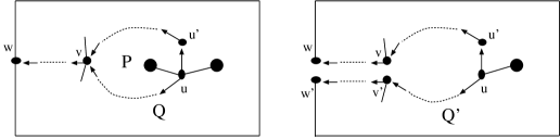
Figure 1: Graph $Q^{\prime}$ obtained from cutting $Q$ along ${\mathop{\rm cp}}(S)$.

Each crest separator $S\in{\cal S}$ decomposes $\hat{G}$ into two pieces $P$ and $Q$ and we assume $P$ is the upper piece and $Q$ is the lower piece. For each edge $e=\{u,v\}$ in ${\mathit{u}p}{\mathop{\rm DDG}}(S)$ (resp. ${\mathit{l}ow}{\mathop{\rm DDG}}(S)$), the weight of $e$ is used to decide whether a minimum face separating cycle should use a shortest path between $u$ and $v$ in $P$ (resp. $Q$) or not, and if so, any shortest path shortest path between $u$ and $v$ in $P$ (resp. $Q$) can be used (there may be multiple shortest paths between $u$ and $v$ in $P$ (resp. $Q$)). So we say edge $\{u,v\}$ in ${\mathit{u}p}{\mathop{\rm DDG}}(S)$ (resp. ${\mathit{l}ow}{\mathop{\rm DDG}}(S)$) represents any shortest path between $u$ and $v$ in $P$ (resp. $Q$). The computation of ${\mathit{u}p}{\mathop{\rm DDG}}(S)$ (resp.${\mathit{l}ow}{\mathop{\rm DDG}}(S)$) also includes computing one shortest path between $u$ and $v$ in $P$ (resp. $Q$) for every edge $\{u,v\}$ in ${\mathit{u}p}{\mathop{\rm DDG}}(S)$ (resp. ${\mathit{l}ow}{\mathop{\rm DDG}}(S)$).

Note that in this paper we use the terms ${\mathit{u}p}{\mathop{\rm DDG}}$ and ${\mathit{l}ow}{\mathop{\rm DDG}}$ instead of the h-high pseudo shortcut set in [27] to give a more clear description.

The following properties of the down paths, GMST $(\hat{G},{\cal S},{\cal W})$, ${\mathit{u}p}{\mathop{\rm DDG}}(S)$ and ${\mathit{l}ow}{\mathop{\rm DDG}}(S)$ can be easily verified and are proved in [27]:

• For any pair of vertices $u$ and $v$ in $\hat{G}$, ${\mathop{\rm dist}}_{\hat{G}}(u,v)\geq|l_{\hat{G}}(u)-l_{\hat{G}}(v)|$.

• For any pair of vertices $u$ and $v$ in a same down path of $S$, ${\mathop{\rm dist}}_{S}(u,v)=|l_{\hat{G}}(u)-l_{\hat{G}}(v)|={\mathop{\rm dist}}_{\hat{G}}(u,v)$.

• If $\hat{G}$ is $O(k)$-outerplanar then for every $S\in{\cal S}$, there are $O(k)$ vertices and $O(k)$ edges in $S$ and every edge in ${\mathit{u}p}{\mathop{\rm DDG}}(S)$ (${\mathit{l}ow}{\mathop{\rm DDG}}(S))$ has weight $O(k)$.

• If $\hat{G}$ is $O(k)$-outerplanar, $\sum_{P_{i}\in T_{\cal{S}}}|E(P_{i})|=|E(\hat{G})|+O(|{\cal{S}}|k)$.

• For every $S\in{\cal S}$ and each edge $e=\{u,v\}$ in ${\mathit{u}p}{\mathop{\rm DDG}}(S)$/${\mathit{l}ow}{\mathop{\rm DDG}}(S)$, any shortest path represented by $e$ contains no vertex of height greater than $l_{\hat{G}}(S)$ and no more than $t-1$ vertices of height $l_{\hat{G}}(S)$, where $t$ is the number of top vertices of $S$.

• Let $S$ be the crest separator on edge $\{P_{i},P_{j}\}$ in $T_{\cal S}$. Assume that $Z_{i}$ and $Z_{j}$ are in the upper piece and lower piece by $S$, respectively. For every edge $e=\{u,v\}$ in ${\mathit{u}p}{\mathop{\rm DDG}}(S)$ (resp. ${\mathit{l}ow}{\mathop{\rm DDG}}(S)$), any shortest path represented by $e$ and the segment of $S$ between $u$ and $v$ that contains a top vertex of $S$ form a cycle which separates $Z_{i}$ (resp. $Z_{j}$) from $f_{0}$.

From Properties (I)-(VI), the ${\mathit{u}p}{\mathop{\rm DDG}}(S)$ and ${\mathit{l}ow}{\mathop{\rm DDG}}(S)$ can be computed as shown in the next lemma (Lemma 18 in [27]).

Lemma 7

[27] Given a GMST $(\hat{G},{\cal S},{\cal W})$, ${\mathit{u}p}{\mathop{\rm DDG}}(S)$ and ${\mathit{l}ow}{\mathop{\rm DDG}}(S)$ for all $S\in{\cal S}$ can be computed in $O(|V(\hat{G})|k^{3})$ time.

The authors of [27] settle for this result because in their application, $|{\cal W}|=O(|V(\hat{G})|)$. However, it is hidden in the proof details and stated in [22] that the time complexity is actually $O(|V(\hat{G})|k+|{\cal W}|k^{3})$. It is also hidden in the details that the Lemma holds when $\hat{G}$ is weighted. We now state Lemma 7 as the following Lemma which will be used in this paper.

Lemma 8

[27, 28] Given a GMST $(\hat{G},{\cal S},{\cal W})$, ${\mathit{u}p}{\mathop{\rm DDG}}(S)$ and ${\mathit{l}ow}{\mathop{\rm DDG}}(S)$ for all $S\in{\cal S}$ can be computed in $O(|V(\hat{G})|k+|{\cal W}|k^{3})$ time.

4.2 Algorithm for Theorem 3

For a level 1 node $X$ and the set ${\cal Z}_{X}$ of child nodes in the layer tree ${\mathop{\rm LT}}(G|U,\partial(U))$ in Procedure Branch-Minor, recall that $G_{X}$ is the plane graph converted from plane hypergraph $(G|\overline{X})|{\cal Z}_{X}$ and $H_{X}$ is the weighted plane graph computed from $G_{X}$ as described in Section 3. Recall that ${\cal W}_{X}=\{Z\in{\cal Z}_{X}\mid|C_{Z}|>k\}$. We apply the techniques in [26, 27] to decompose $H_{X}$ into pieces, each piece contains face $f_{Z}$ of $H_{X}$ for exactly one $Z\in{\cal W}_{X}$. It may not be straightforward to decompose $H_{X}$ directly by the techniques of [26, 27] because some of the techniques are described for graphs while $H_{X}$ is weighted (edges have weight $1/2$ or 1). To get a decomposition of $H_{X}$ as required, we first construct an almost triangulated graph $\hat{G}_{X}$ from $G_{X}$ with each $Z\in{\cal Z}_{X}$ represented by a crest of $\hat{G}_{X}$; then by the techniques of [26, 27] find a GMST of $\hat{G}_{X}$ which decomposes $\hat{G}_{X}$ into pieces, each piece contains exactly one crest; next construct an almost triangulated weighted graph $\hat{H}_{X}$ from $H_{X}$ with each $Z\in{\cal Z}_{X}$ represented by a crest of $\hat{H}_{X}$; and finally compute a set of crest separators in $\hat{H}_{X}$ based on the GMST of $\hat{G}_{X}$ to decompose $\hat{H}_{X}$ into pieces such that each piece $\hat{H}_{X}$ contains exactly one crest $Z\in{\cal W}_{X}$ (and thus each piece of $H_{X}$ contains exactly one face $f_{Z}$).

We first describe the construction of $\hat{G}_{X}$. Let $f_{\overline{X}}$ be the outer face of $G_{X}$. For every $Z\in{\cal Z}_{X}$, we add a vertex, also denoted by $Z$, and edges $\{u,Z\}$ for every $u\in V(f_{Z})$ to face $f_{Z}$ in $G_{X}$. For every natural face $f$ of $G_{X}$ with $|V(f)|>3$, we select an arbitrary vertex $v$ of $V(f)$ with $l_{G_{X}}(v)=l_{G_{X}}(f)$ as the low-point of $f$, denoted by ${\mathop{\rm lp}}(f)$, and we add edges $\{u,{\mathop{\rm lp}}(f)\}$ to face $f$ for every $u\in V(f)$ and not adjacent to ${\mathop{\rm lp}}(f)$. Let $\hat{G}_{X}$ be the graph obtained from adding the vertices and edges above. Let $f_{\overline{X}}$ be the outer face of $\hat{G}_{X}$. Then $\hat{G}_{X}$ is almost triangulated.

$G_{X}$ is a subgraph of $\hat{G}_{X}$. For every $u\in V(G_{X})\cap V(\hat{G}_{X})$, $l_{G_{X}}(u)=l_{\hat{G}_{X}}(u)$, every vertex $Z$ added to face $f_{Z}$ of $G_{X}$ is a crest of $\hat{G}_{X}$ and every crest of $\hat{G}_{X}$ is a vertex $Z$ added to $f_{Z}$. Recall that ${\cal W}_{X}=\{Z\in{\cal Z}_{X}\mid|C_{Z}|>k\}$ which is a subset of crests in $\hat{G}_{X}$. By Lemma 6, we can find a GMST $(\hat{G}_{X},{\cal S},{\cal W}_{X})$.

Next we describe how to construct $\hat{H}_{X}$. For every $Z\in{\cal Z}_{X}$, we add a vertex, also denoted by $Z$, and edges $\{u,Z\}$ for every $u\in V(f_{Z})$ to face $f_{Z}$ of $H_{X}$. We assign each edge $\{u,Z\}$ weight $1$. Let $\hat{H}_{X}$ be the graph computed above and $f_{\overline{X}}$ be the outer face of $\hat{H}_{X}$. Then $\hat{H}_{X}$ is almost triangulated. Notice that $V(G_{X})\subseteq V(\hat{G}_{X})\subseteq V(\hat{H}_{X})$, $V(H_{X})\subseteq V(\hat{H}_{X})$, $E(G_{X})\subseteq E(\hat{G}_{X})$, $E(G_{X})\subseteq E(H_{X})\subseteq E(\hat{H}_{X})$ and $|V(\hat{H}_{X})|=O(|V(G_{X})|)$. We define the height $l_{\hat{H}_{X}}(u)$ of each vertex $u$ of $\hat{H}_{X}$ as follows:

• $l_{\hat{H}_{X}}(u)=l_{G_{X}}(u)$ if $u\in V(\hat{H}_{X})\cap V(G_{X})$.

• $l_{\hat{H}_{X}}(u)=l_{G_{X}}(f)+1/2$ if $u=u_{f}$ is the vertex added to a natural face $f$ of $G_{X}$.

• $l_{\hat{H}_{X}}(u)=l_{G_{X}}(f_{Z})+1$ if $u=Z$ is the vertex added to $f_{Z}$.

Then each vertex $Z$ is a crest of $\hat{H}_{X}$ and each crest of $\hat{H}_{X}$ is a vertex $Z$. The heights of a face and a crest separator, and the depth of a ridge in $\hat{H}_{X}$ are defined based on $l_{\hat{H}_{X}}(u)$ similarly as those in Section 4.1.

Similar to the down vertex and down edge in $\hat{G}_{X}$, we define the down vertex and down edge for each vertex of $\hat{H}_{X}$. Recall that any vertex $v$ adjacent to vertex $u$ with $l_{\hat{H}_{X}}(v)<l_{\hat{H}_{X}}(u)$ can be selected as the down vertex of $u$. We choose the down vertex for each $u$ of $\hat{H}_{X}$ as follows:

• if $u\in V(\hat{G}_{X})$ and the down edge $\{u,v\}$ in $\hat{G}_{X}$ is an edge of $G_{X}$ or an edge added to face $f_{Z}$ ($u$ is a crest) then $v$ is the down vertex of $u$ in $\hat{H}_{X}$;

• if $u\in V(\hat{G}_{X})$ and the down edge $\{u,v\}$ in $\hat{G}_{X}$ is an edge added to a natural face $f$ of $G_{X}$ then the vertex $u_{f}$ added to $f$ in $\hat{H}_{X}$ is the down vertex of $u$; and

• otherwise, $u$ is not in $\hat{G}_{X}$ and is the vertex $u_{f}$ added to a natural face $f$ of $G_{X}$ in $\hat{H}_{X}$; then the low-point ${\mathop{\rm lp}}(f)$ is the down vertex of $u$.

The edge between vertex $u$ and its down vertex is the down edge of $u$.

Given a GMST $(\hat{G}_{X},{\cal S},{\cal W}_{X})$, for every crest separator $S\in{\cal S}$ and every edge $e$ of $S$, either $e\in E(G_{X})\cap E(\hat{G}_{X})$ or $e$ is an edge added to a natural face $f$ of $G_{X}$ during the construction of $\hat{G}_{X}$. We convert each $S\in{\cal S}$ into a subgraph $D$ of $\hat{H}_{X}$: for every edge $e=\{u,v\}$ in $S$, $\{u,v\}$ of $\hat{H}_{X}$ is included in $D$ if $e\in E(G_{X})\cap E(\hat{G}_{X})$, otherwise edges $\{u,u_{f}\},\{u_{f},v\}$ of $\hat{H}_{X}$ are included in $D$, where $u_{f}$ is the vertex added to face $f$ of $G_{X}$ when $H_{X}$ is created from $G_{X}$.

A crest separator $S\in{\cal S}$ for crests $Z$ and $Z^{\prime}$ consists of two paths $L_{1}$ and $L_{2}$ ($L_{1}$ is the down path of some vertex $u$ and $L_{2}$ is composed of the top edge $\{u,u^{\prime}\}$ and the down path of $u^{\prime}$, where $u^{\prime}$ is not in $L_{1}$ and $l_{\hat{G}_{X}}(u^{\prime})\leq l_{\hat{G}_{X}}(u)$) and decomposes $\hat{G}_{X}$ into two pieces, one contains $Z$ and the other contains $Z^{\prime}$. From the way we define the down vertex of every vertex $u$ in $\hat{H}_{X}$, the subgraph $D$ converted from $S$ is also a crest separator consisting of two paths $L^{\prime}_{1}$ and $L^{\prime}_{2}$ in $\hat{H}_{X}$ described below:

• if the top edge $\{u,u^{\prime}\}$ of $S$ is an edge of $G_{X}$ then $L^{\prime}_{1}$ is the down path from vertex $u$ and $L^{\prime}_{2}$ is composed of the top edge $\{u,u^{\prime}\}$ and the down path from $u^{\prime}$;

• if $\{u,u^{\prime}\}$ is an added edge to a natural face $f$ of $G_{X}$ when constructing $\hat{G}_{X}$ and $l_{\hat{G}_{X}}(u)=l_{\hat{G}_{X}}(u^{\prime})+1$ then $L^{\prime}_{1}$ is the down path from vertex $u$ and $L^{\prime}_{2}$ is composed of the top edge $\{u,u_{f}\}$ and the down path from $u_{f}$, where $u_{f}$ is the vertex added to $f$ when constructing $H_{X}$ and $l_{\hat{H}_{X}}(u_{f})=l_{\hat{H}_{X}}(u)-1/2$;

• otherwise ($\{u,u^{\prime}\}$ is an added edge to $f$ and $l_{\hat{G}_{X}}(u)=l_{\hat{G}_{X}}(u^{\prime})$), $L^{\prime}_{1}$ is the down path from vertex $u_{f}$ (added to $f$ when constructing $H_{X}$) and $L^{\prime}_{2}$ is composed of the top edge $\{u_{f},{\mathop{\rm lp}}(f)\}$ and the down path from ${\mathop{\rm lp}}(f)$, where ${\mathop{\rm lp}}(f)=u$ or ${\mathop{\rm lp}}(f)=u^{\prime}$.

In Case (1) and Case (2), $D$ is a crest separator for $Z$ and $Z^{\prime}$. In Case (3), either $D$ intersects a ridge $R$ between $Z$ and $Z^{\prime}$ but $l_{\hat{H}_{X}}(u_{f})=d_{\hat{H}_{X}}(R)+1/2=l_{\hat{H}_{X}}(u)+1/2$ or $D$ is on a ridge $R$ between $Z$ and $Z^{\prime}$ and $l_{\hat{H}_{X}}(D)=l_{\hat{H}_{X}}(u_{f})=d_{\hat{H}_{X}}(R)$. In all cases, $D$ is a crest separator which decomposes $\hat{H}_{X}$ into two pieces $P$ and $Q$, $P$ contains $Z$ and $Q$ contains $Z^{\prime}$.

Let ${\cal D}=\{D|D\mbox{ is converted from $S$ for every $S\in{\cal S}$}\}$ and assume that ${\cal W}_{X}$ has $r$ crests $Z_{1},..,Z_{r}$. It is easy to see that ${\cal D}$ has the following properties:

• The crest separators of ${\cal D}$ decompose $\hat{H}_{X}$ into $r$ pieces $P_{1},...,P_{r}$ such that each piece $P_{i}$ has exactly one crest $Z_{i}$. Moreover, no crest separator $D$ in ${\cal D}$ contains a crest in ${\cal W}_{X}$, that is, each piece contains the edges in $E(f_{Z})$ of $H_{X}$ for exactly one $Z\in{\cal W}_{X}$.

• For each pair of pieces $P_{i}$ and $P_{j}$, there is a crest separator $D\in{\cal D}$ such that $D$ decomposes $\hat{H}_{X}$ into two pieces $P$ and $Q$, $P$ contains $Z_{i}$ and $Q$ contains $Z_{j}$.

  Let ${\cal D}_{ij}$ be the set of crest separators for $Z_{i}$ and $Z_{j}$ in $\hat{H}_{X}$. Recall that every crest separator for $Z_{i}$ and $Z_{j}$ is on a ridge between $Z_{i}$ and $Z_{j}$ and thus all crest separators in ${\cal D}_{ij}$ have the same height, denoted as $l_{\hat{H}_{X}}({\cal D}_{ij})$. For $D$ in Case (1), Case (2) and Case (3) with $l_{\hat{H}_{X}}(u_{f})=d_{\hat{H}_{X}}(R)=l_{\hat{H}_{X}}({\cal D}_{ij})$, from Property (B), we have

  (B1) $D$ is in ${\cal D}_{ij}$ and has the minimum number of top vertices among all crest separators in ${\cal D}_{ij}$.

  For $D$ in Case (3) with $l_{\hat{H}_{X}}(u_{f})=d_{\hat{H}_{X}}(R)+1/2$,

  (B2) $D$ is not in ${\cal D}_{ij}$, $l_{\hat{H}_{X}}(D)=l_{\hat{H}_{X}}({\cal D}_{ij})+1/2$ and every crest separator in ${\cal D}_{ij}$ has two top vertices.

• Let $T_{\cal D}$ be the graph that $V(T_{\cal D})=\{P_{1},...,P_{r}\}$ and there is an edge $\{P_{i},P_{j}\}\in E(T_{\cal D})$ if there is a crest separator $D=E(P_{i})\cap E(P_{j})$ in ${\cal D}$. Then $T_{\cal D}$ is a tree.

The tuple $(\hat{H}_{X},{\cal D},{\cal W}_{X})$ is called a pseudo good mountain structure tree (pseudo GMST) for ${\cal W}_{X}$. For each $D\in{\cal D}$ and vertices $u,v$ of $D$, ${\mathop{\rm dist}}_{D}(u,v)$, ${\mathit{u}p}{\mathop{\rm DDG}}(D)$ and ${\mathit{l}ow}{\mathop{\rm DDG}}(D)$ are defined similarly as ${\mathop{\rm dist}}_{S}(u,v)$, ${\mathit{u}p}{\mathop{\rm DDG}}(S)$ and ${\mathit{l}ow}{\mathop{\rm DDG}}(S)$ for crest separator $S$ and $u,v$ of $S$ in Section 4.1. As shown in the next lemma, Properties (I)-(VI) in Section 4.1 hold for a pseudo GMST, ${\mathit{u}p}{\mathop{\rm DDG}}(D)$ and ${\mathit{l}ow}{\mathop{\rm DDG}}(D)$.

Lemma 9

Properties (I)-(VI) hold for a pseudo GMST $(\hat{H}_{X},{\cal D},{\cal W}_{X})$, ${\mathit{u}p}{\mathop{\rm DDG}}(D)$ and ${\mathit{l}ow}{\mathop{\rm DDG}}(D)$, $D\in{\cal D}$.

Proof:  Property (I) and Property (II) hold trivially from the definition of $l_{\hat{H}_{X}}(u)$ for vertex $u$ and the definition of down path.

If $\hat{H}_{X}$ is $O(k)$-outerplanar, then the height of $D$ is $O(k)$ and there are $O(k)$ vertices and $O(k)$ edges in $D$ because the weight of each edge in $\hat{H}_{X}$ is $1$ or $1/2$. From Property (II), every edge in ${\mathit{u}p}{\mathop{\rm DDG}}(D)$ (${\mathit{l}ow}{\mathop{\rm DDG}}(D))$ has weight $O(k)$ because ${\mathop{\rm dist}}_{D}(u,v)=O(k)$ for any $u$ and $v$ in $D$. Thus, Property (III) holds.

Every $D\in{\cal D}$ is converted from an $S\in{\cal S}$ and $|E(D)|=O(|E(S)|)$. From this, and $|{\cal D}|=|{\cal S}|$, $\sum_{P_{i}\in T_{\cal{D}}}|E(P_{i})|=|E(\hat{H}_{X})|+O(|{\cal{D}}|k)$. Thus, Property (IV) holds.

From Property (II), for each edge $e=\{u,v\}$ in ${\mathit{u}p}{\mathop{\rm DDG}}(S)$/${\mathit{l}ow}{\mathop{\rm DDG}}(S)$, $u$ and $v$ must be in different down paths of $D$ and ${\mathop{\rm dist}}_{D}(u,v)=2l_{\hat{H}_{X}}(D)-l_{\hat{H}_{X}}(u)-l_{\hat{H}_{X}}(v)+(t-1)$, where $t\in\{1,2\}$ is the number of top vertices of $D$. Any vertex $w$ of height greater than $l_{\hat{H}_{X}}(D)$ in $\hat{H}_{X}$ has height at least $l_{\hat{H}_{X}}(D)+1/2$. From Property (I), any path between $u$ and $v$ that contains $w$ has length at least $2l_{\hat{H}_{X}}(D)+1-l_{\hat{H}_{X}}(u)-l_{\hat{H}_{X}}(v)\geq{\mathop{\rm dist}}_{D}(u,v)$. Similarly, any path between $u$ and $v$ that contains $t$ vertices of height $l_{\hat{H}_{X}}(D)$ has length at least ${\mathop{\rm dist}}_{D}(u,v)$. Therefore, any path represented by $e$ contains no vertex of height greater than $l_{\hat{H}_{X}}(D)$ and no more than $t-1$ vertices of height $l_{\hat{H}_{X}}(D)$ since its length is strictly smaller than ${\mathop{\rm dist}}_{D}(u,v)$. Thus, Property (V) holds.

We prove Property (VI) by contradiction. Let $D\in{\cal D}$ be the crest separator on edge $\{P_{i},P_{j}\}$ in $T_{\cal D}$. We assume that $Z_{i}$ and $Z_{j}$ are in the upper piece and lower piece by $D$ respectively. For each edge $e=\{u,v\}$ in ${\mathit{u}p}{\mathop{\rm DDG}}(D)$ (resp. ${\mathit{l}ow}{\mathop{\rm DDG}}(D)$), let $P_{e}$ be any shortest path in the upper piece (resp. lower piece) represented by $e$ and let $D(u,v)$ be the segment of $D$ between $u$ and $v$ and containing a top vertex of $D$. Then $P_{e}$ and $D(u,v)$ form a cycle in $\hat{H}_{X}$. Assume for contradiction that the cycle formed by $P_{e}$ and $D(u,v)$ does not separate $Z_{i}$ (resp. $Z_{j}$) from $f_{\overline{X}}$. Let ${\cal D}_{ij}$ be the set of crest separators for $Z_{i}$ and $Z_{j}$ as defined in Property (B). Let $D^{\prime}$ be the subgraph of $\hat{H}_{X}$ obtained by replacing $D(u,v)$ with $P_{e}$ in $D$. Then $D^{\prime}$ separates $Z_{i}$ from $Z_{j}$ and thus, intersects with every ridge between $Z_{i}$ and $Z_{j}$. Since each ridge between $Z_{i}$ and $Z_{j}$ has depth $l_{\hat{H}_{X}}({\cal D}_{ij})$, $D^{\prime}$ contains at least one vertex $w$ with $l_{\hat{H}_{X}}(w)=l_{\hat{H}_{X}}({\cal D}_{ij})$. Notice that no vertex of $D^{\prime}\setminus P_{e}$ has height $l_{\hat{H}_{X}}({\cal D}_{ij})$. So $P_{e}$ contains $w$. Consider Case (B1) in Property (B) where $D\in{\cal D}_{ij}$ and $D$ has the minimum number of top vertices among all crest separators in ${\cal D}_{ij}$. If $D$ has exactly one top vertex, from Property (V), $P_{e}$ contains no vertex of height $l_{\hat{H}_{X}}({\cal D}_{ij})$, a contradiction. If $D$ has two top vertices then every crest separator in ${\cal D}_{ij}$ (for $Z$ and $Z^{\prime}$) has two top vertices and $w$ is the only vertex of height $l_{\hat{H}_{X}}({\cal D}_{ij})$ in $P_{e}$. However, this means that there is a crest separator for $Z_{i}$ and $Z_{j}$ with exactly one top vertex $w$, a contradiction. Consider Case (B2) where $l_{\hat{H}_{X}}(D)=l_{\hat{H}_{X}}({\cal D}_{ij})+1/2$, and every crest separator in ${\cal D}_{ij}$ has two top vertices. As proved, if $P_{e}$ has exactly one vertex of height $l_{\hat{H}_{X}}({\cal D}_{ij})$, we have a contradiction. If $P_{e}$ has two vertices of height greater than or equal to $l_{\hat{H}_{X}}({\cal D}_{ij})$, the length of $P_{e}$ is not strictly smaller than the length of ${\mathop{\rm dist}}_{D}(u,v)$, a contradiction. This gives Property (VI). $\Box$

Given a GMST $(\hat{G}_{X},{\cal S},{\cal W}_{X})$, a pseudo GMST $(\hat{H}_{X},{\cal D},{\cal W}_{X})$ can be computed in $O(|{\cal S}|k)$ time. Lemma 7 and Lemma 8 hold for a pseudo GMST because the lemmas only rely on Properties (I)-(VI). The computation of ${\mathit{u}p}{\mathop{\rm DDG}}(D)$ and ${\mathit{l}ow}{\mathop{\rm DDG}}(D)$ in Lemma 7 and Lemma 8 (implicitly) uses a linear time algorithm by Thorup [37] for the single shortest path problem in graphs with integer edge weight as a subroutine. This requires that the edge weight in $\hat{H}_{X}$, ${\mathit{u}p}{\mathop{\rm DDG}}(D)$ and ${\mathit{l}ow}{\mathop{\rm DDG}}(D)$ can be expressed in $O(1)$ words in integer form. So the perturbation technique used in Section 3 cannot be used in the computation above. In the algorithm for Theorem 3, we do not assume the uniqueness of shortest paths when we compute minimum separating cycles. A minimum $(f_{Z},f_{\overline{X}})$-separating cycle $C$ cuts $\Sigma$ into two regions, one contains $f_{Z}$ and the other contains $f_{\overline{X}}$. Let ${\mathop{\rm ins}}(C)$ be the region containing $f_{Z}$. We say two cycles $C$ and $C^{\prime}$ cross with each other if ${\mathop{\rm ins}}(C)\cap{\mathop{\rm ins}}(C^{\prime})\neq\emptyset$, ${\mathop{\rm ins}}(C)\setminus{\mathop{\rm ins}}(C^{\prime})\neq\emptyset$ and ${\mathop{\rm ins}}(C^{\prime})\setminus{\mathop{\rm ins}}(C)\neq\emptyset$. We say a set of at least two cycles are crossing if for any cycle $C$ in this set, there is at least one other cycle $C^{\prime}$ that crosses with $C$. In Section 3, we do not have crossing minimum separating cycles because of the uniqueness of shortest paths. However, two minimum separating cycles computed without the assumption of unique shortest paths may cross with each other. We eliminate each crossing cycle set by exploiting some new properties of pseudo GMST, ${\mathit{u}p}{\mathop{\rm DDG}}(D)$ and ${\mathit{l}ow}{\mathop{\rm DDG}}(D)$, and then compute a good separator for ${\cal A}_{X}$.

Recall that $\hat{H}_{X}$ is constructed from $H_{X}$ by adding vertex (crest) $Z$ and edges $\{u,Z\}$, $u\in V(f_{Z})$, to face $f_{Z}$ in $H_{X}$. Each piece $P$ of a pseudo GMST $(\hat{H}_{X},{\cal D},{\cal W}_{X})$ contains exactly one crest $Z\in{\cal W}_{X}$. By Property (A), removing $Z$ and the edges incident to $Z$ from piece $P$ gives a piece of $H_{X}$ containing face $f_{Z}$ for exactly one $Z\in{\cal W}_{X}$. From this and further Property (A) and Property (V), we will show in the proof of Lemma 10 that a minimum $(f_{Z},f_{\overline{X}})$-separating cycle can be computed based on $(\hat{H}_{X},{\cal D},{\cal W}_{X})$, ${\mathit{u}p}{\mathop{\rm DDG}}(D)/{\mathit{l}ow}{\mathop{\rm DDG}}(D)$, $D\in{\cal D}$, and the approaches of [12, 30].

Given a set ${\cal W}_{X}$ of crests in $\hat{H}_{X}$, our algorithm for Theorem 3 computes a pseudo GMST $(\hat{H}_{X},{\cal D},{\cal W}_{X})$, calculates ${\mathit{u}p}{\mathop{\rm DDG}}(D)$ and ${\mathit{l}ow}{\mathop{\rm DDG}}(D)$ for every crest separator $D\in{\cal D}$, and finds a minimum $(f_{Z},f_{\overline{X}})$-separating cycle for every $Z\in{\cal W}_{X}$ using the pseudo GMST, ${\mathit{u}p}{\mathop{\rm DDG}}(D)$ and ${\mathit{l}ow}{\mathop{\rm DDG}}(D)$. More specifically, we replace Steps 2(b)(c) in Procedure Branch-Minor with the following subroutine to get an algorithm for Theorem 3.
Subroutine Crest-Separator
Input: Hypergraph $(G|\overline{X})|{\cal Z}_{X}$, weighted graph $H_{X}$ and integer $k$.
Output: Good separator ${\mathcal{A}}_{X}$ for ${\cal Z}_{X}$ and $\overline{X}$ or a $(k+1)\times\lceil{\frac{k+1}{2}}\rceil$ cylinder minor.

1. For every $Z\in{\cal Z}_{X}$ with $|C_{Z}|\leq k$, take $C_{Z}$ as a $(f_{Z},f_{\overline{X}})$-separating cycle and mark $Z$ as separated.

2. Compute $\hat{G}_{X}$ and $\hat{H}_{X}$. Let ${\cal W}_{X}=\{Z\in{\cal Z}_{X}\mid|C_{Z}|>k\}$.

3. Compute a GMST $(\hat{G}_{X},{\cal S},{\cal W}_{X})$ by Lemma 6 and a pseudo GMST $(\hat{H}_{X},{\cal D},{\cal W}_{X})$ from $(\hat{G}_{X},{\cal S},{\cal W}_{X})$.

4. Compute ${\mathit{u}p}{\mathop{\rm DDG}}(D)$ and ${\mathit{l}ow}{\mathop{\rm DDG}}(D)$ for every crest separator $D\in{\cal D}$ by Lemma 8.

5. Mark every $Z\in{\cal W}_{X}$ as un-separated. Repeat the following until every $Z$ is marked as separated.

   1. Choose an arbitrary un-separated $Z$, compute a minimum $(f_{Z},f_{\overline{X}})$-separating cycle $C$ using the pseudo GMST $(\hat{H}_{X},{\cal D},{\cal W})$, ${\mathit{u}p}{\mathop{\rm DDG}}(D)$ and ${\mathit{l}ow}{\mathop{\rm DDG}}(D)$. We call $C$ the cycle computed for $Z$.

   2. If the length of $C$ is greater than $k$ then compute a $(k+1)\times\lceil{\frac{k+1}{2}}\rceil$ cylinder minor by Lemma 1 and terminate. Otherwise, take this cycle as the minimum $(f_{Z},f_{\overline{X}})$-separating cycle for every $Z\in{\mathop{\rm ins}}(C)$ and mark every $Z$ in ${\mathop{\rm ins}}(C)$ separated.

6. Compute ${\mathcal{A}}_{X}$ from the (minimum) face separating cycles obtained in Step (1) and Step (5).

We now analyze the time complexity of Subroutine Crest-Separator.

Lemma 10

Steps (1)-(5) of Subroutine Crest-Separator can be computed in $O(|E(H_{X})|k^{2})$ time.

Proof:  Let $m$ be the numbers of edges in $H_{X}$. Then $|E(\hat{H}_{X})|=O(m)$. Notice that each edge of $\hat{H}_{X}$ appears in at most one boundary cycle $C_{Z}$ because any pair of boundary cycles do not have more than one common vertex. From this, $\sum_{Z\in{\mathcal{Z}_{X}}}|C_{Z}|=O(m)$. Therefore, for all $Z\in{\cal Z}_{X}\setminus{\cal W}_{X}$, $(f_{Z},f_{\overline{X}})$-separating cycles can be found in $O(m)$ time. For each crest $Z\in{\cal W}_{X}$, $C_{Z}$ has more than $k$ edges in $H_{X}$. Therefore, $|{\cal W}_{X}|=O(m/k)$. A pseudo GMST $(\hat{H}_{X},{\cal D},{\cal W}_{X})$, ${\mathit{u}p}{\mathop{\rm DDG}}(D)$ and ${\mathit{l}ow}{\mathop{\rm DDG}}(D)$ for all $D\in\cal{D}$ can be computed in $O(mk+|{\cal W}_{X}|k^{3})=O(mk^{2})$ time (Lemmas 6 and 8).

For an un-separated crest $Z\in{\cal W}_{X}$, let $P$ be the piece in the pseudo GMST $(\hat{H}_{X},{\cal D},{\cal W}_{X})$ containing $Z$ (see Figure 2 (a)). By Property (A), removing $Z$ and the edges incident to $Z$ from $P$ gives a piece $P^{\prime}$ of $H_{X}$ containing face $f_{Z}$ of $H_{X}$ (see Figure 2 (b)). Let $x$ be an arbitrary vertex in $P$ incident to $Z$ and $L$ be the down path from $x$ to a vertex $w\in V(f_{\overline{X}})$. Then $L$ is a shortest path between $x$ and $w$ in $H_{X}$ and can be found in $O(k)$ time. Let $P(L)$ be the weighted plane graph obtained from $P^{\prime}$ by cutting along $L$: for each vertex $u$ in $L$ create a duplicate $u^{\prime}$, for each edge $e$ in $L$ create a duplicate $e^{\prime}$ and create a new face bounded by edges of $E(f_{\overline{X}})$, $E(f_{Z})$, $L$ and their duplicates (see Figure 2 (c)). Let $H_{X}(L)$ be the weighted graph obtained from $H_{X}$ by replacing $P^{\prime}$ with $P(L)$. For each vertex $u$ in path $L$, let $C_{u}$ be a shortest path between $u$ and its duplicate $u^{\prime}$ in $H_{X}(L)$. Let $y$ be a vertex in $L$ such that $C_{y}$ has the minimum length among the paths $C_{u}$ for all vertices $u$ in $L$. Then $C_{y}$ gives a minimum $(f_{Z},f_{\overline{X}})$-separating cycle in $H_{X}$ [30].

Figure 2: (a) Piece $P$ of $\hat{H}_{X}$, (b) piece $P^{\prime}$ of $H_{X}$ and (c) graph $P(L)$.

For each piece $P$ in pseudo GMST $(\hat{H}_{X},{\cal D},{\cal W}_{X})$, let $\tilde{D}$ be the crest separator on the edge between $P$ and its parent node and let ${\cal D}_{P}$ be the set of crest separators on an edge between $P$ and a child node of $P$ in $T_{\cal D}$. From Property (A) and Property (V), any shortest path represented by an edge in ${\mathit{u}p}{\mathop{\rm DDG}}(D)$ or ${\mathit{l}ow}{\mathop{\rm DDG}}(D)$, $D\in{\cal D}$, does not contain any vertex of $V(\hat{H}_{X})\setminus V(H_{X})$. Therefore, $C_{u}$ for every $u$ in $L$ can be partitioned into subpaths such that each subpath is either entirely in $P(L)$ or is represented by an edge in ${\mathit{u}p}{\mathop{\rm DDG}}(\tilde{D})$ or ${\mathit{l}ow}{\mathop{\rm DDG}}(D)$, $D\in{\cal D}_{P}$. Let $P^{*}$ be the weighted graph consisting of the edges of $P(L)$, ${\mathit{u}p}{\mathop{\rm DDG}}(\tilde{D})$ and ${\mathit{l}ow}{\mathop{\rm DDG}}(D)$, $D\in{\cal D}_{P}$. Notice that for every edge $e$ in ${\mathit{u}p}{\mathop{\rm DDG}}(\tilde{D})$ and ${\mathit{l}ow}{\mathop{\rm DDG}}(D)$, $D\in{\cal D}_{P}$, a shortest path represented by $e$ is also computed. Then it is known (Section 2.2 in [12]) that a $C_{y}$ can be computed in $O(t(P^{*})\log|V(L)|+|V(C_{y})|)=O(t(P^{*})\log k+|V(C_{y})|)$ time, where $t(P^{*})$ is the time to find a shortest path $C_{u}$ in $P^{*}$ for any $u$ in $L$. For each edge of $P^{*}$, we can multiply the edge weight by 2 to make each edge weight a positive integer. By the algorithm in [37], a shortest path $C_{u}$ can be computed in linear time, that is, $t(P^{*})=O(|E(P^{*})|)$. Therefore, from the fact that each crest separator has $O(k)$ vertices (Property III), it takes

$$O((|E(P(L))|+|E({\mathit{u}p}{\mathop{\rm DDG}}(\tilde{D}))|+|\cup_{D\in\cal{D}_{P}}E({\mathit{l}ow}{\mathop{\rm DDG}}(D))|)\log k+|V(C_{y})|)$$

$$= O((|E(P)|+\Delta(P)k^{2})\log k+|V(C_{y})|)$$

time to compute a minimum $(f_{Z},f_{\overline{X}})$-separating cycle, where $\Delta(P)$ is the number of edges incident to $P$ in $T_{\cal D}$. If $C_{y}$ has length at most $k$ then $|V(C_{y})|=O(k)$, otherwise $|V(C_{y})|=O(m)$. Assume that $C_{y}$ for every $Z\in{\cal W}_{X}$ has length at most $k$. From Property (C), Property (IV) and $|V(T_{\cal D})|=|{\cal W}_{X}|=O(m/k)$, the time for computing the minimum $(f_{Z},f_{\overline{X}})$-separating cycles for all crests $Z\in{\cal W}_{X}$ is

$$\sum_{P\in V(T_{\cal D})}O((|E(P)|+\Delta(P)k^{2})\log k+k) = O((m+|{\cal W}_{X}|k+|{\cal W}_{X}|k^{2})\log k+|{\cal W}_{X}|k)$$

$$= O(mk\log k).$$

If there is a $C_{y}$ with length greater than $k$, it takes

$$O((|E(P)|+\Delta(P)k^{2})\log k+m)=O(mk\log k)$$

time to compute this $C_{y}$. After the first $C_{y}$ with length greater than $k$ is computed, the subroutine computes a cylinder minor in $O(m)$ time and terminates.

Summing up, the total time for Steps (1)-(5) is $O(|E(H_{X})|k^{2})$. $\Box$

Any two boundary cycles do not cross with each other because they do not share any common edge, each boundary cycle is the boundary of a face of $G_{X}$ and the faces are disjoint. The height of any vertex in a boundary cycle is no smaller than the height of any $D\in{\cal D}$. Therefore from Property (B) and Property (V), a boundary cycle does not cross with a minimum separating cycle for a crest $Z$. However, a minimum separating cycle for one crest may cross with a minimum separating cycle for another crest. The next lemma gives a base for eliminating crossing separating cycles.

Lemma 11

Let $C_{1}$ be the minimum $(f_{Z},f_{\overline{X}})$-separating cycle computed for crest $Z$ in Step (5). Let $C_{2}$ be the minimum $(f_{Z^{\prime}},f_{\overline{X}})$-separating cycle computed for crest $Z^{\prime}$ after $C_{1}$ in step (5). If $C_{1}$ and $C_{2}$ cross with each other, then there is a cycle $C$ such that ${\mathop{\rm ins}}(C)={\mathop{\rm ins}}(C_{1})\cup{\mathop{\rm ins}}(C_{2})$ and the length of $C$ is the same as that of $C_{2}$.

Proof:  Assume that $P_{1}$ and $P_{l}$ in the underlying tree $T_{\cal D}$ contain $Z$ and $Z^{\prime}$, respectively. Let $\{P_{1},P_{2}\},\{P_{2},P_{3}\},...,\{P_{l-1},P_{l}\}$ be the path between $P_{1}$ and $P_{l}$ in $T_{\cal D}$ and let the crest in $P_{i}$ be $Z_{i}$ for $1\leq i\leq l$ ($Z=Z_{1}$ and $Z^{\prime}=Z_{l}$). It is shown in [27] (Lemma 30) that if $Z_{i}\in{\mathop{\rm ins}}(C_{1})$ then every $Z_{j}\in{\mathop{\rm ins}}(C_{1})$ for $j<i$, and if $Z_{i}\in{\mathop{\rm ins}}(C_{2})$ then every $Z_{j}\in{\mathop{\rm ins}}(C_{2})$ for $j>i$. From this and the fact that $C_{2}$ is computed after $C_{1}$, which means $Z^{\prime}\notin{\mathop{\rm ins}}(C_{1})$, there is a $Z_{i}$, $1\leq i<l$, such that $Z_{i}\in{\mathop{\rm ins}}(C_{1})$ but $Z_{j}\not\in{\mathop{\rm ins}}(C_{1})$ for $j>i$.

Let $D$ be the crest separator for $Z_{i}$ and $Z_{i+1}$ in the pseudo GMST (see Figure 3). We assume without loss of generality that $Z$ (resp. $Z^{\prime}$) is in the upper (resp. lower) piece by $D$. From Property (VI) and the fact that $Z_{i+1}\notin{\mathop{\rm ins}}(C_{1})$, $C_{1}$ contains no (shortest path represented by) edge in ${\mathit{l}ow}{\mathop{\rm DDG}}(D)$. Note that $D$ separates $Z$ from $Z^{\prime}$ in $\hat{H}_{X}$. From the fact that $C_{1}$ and $C_{2}$ cross with each other and the fact that $C_{1}$ contains no edge in ${\mathit{l}ow}{\mathop{\rm DDG}}(D)$, $C_{2}$ has a subpath $C_{2}(u,v)$ represented by an edge $e=\{u,v\}$ in ${\mathit{u}p}{\mathop{\rm DDG}}(D)$, where $u$ and $v$ are in different down paths of $D$.

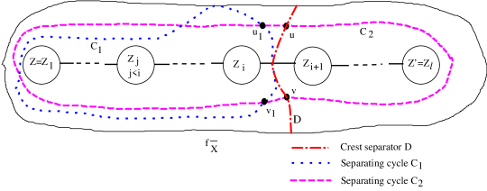
Figure 3: A pair of crossing minimum separating cycles $C_{1}$ and $C_{2}$.

Since $C_{1}$ and $C_{2}$ cross with each other, they intersect at at least two vertices. Let $u_{1}$ and $v_{1}$ be the first vertex and last vertex at which cycle $C_{2}$ intersects cycle $C_{1}$, respectively, when we proceed on $C_{2}(u,v)$ from $u$ to $v$ (see Figure 3). Let $C_{2}(u_{1},v_{1})$ be the subpath of $C_{2}(u,v)$ connecting $u_{1}$ and $v_{1}$. Because $C_{1}$ separates $Z_{i}$ from $Z_{i+1}$, it must contain a subpath $C_{1}(u_{1},v_{1})$ which connects $u_{1}$ and $v_{1}$ and intersects the ridge between $Z_{i}$ and $Z_{i+1}$. Let $C_{2}(u,u_{1})$ (resp. $C_{2}(v,v_{1})$) be the subpath of $C_{2}(u,v)$ between $u$ and $u_{1}$ (resp. $v$ and $v_{1}$). Then the length of $C_{2}(u,v)$ is the sum of the lengths of $C_{2}(u,u_{1})$, $C_{2}(u_{1},v_{1})$ and $C_{2}(v,v_{1})$. Let $D(u,v)$ be the subpath of $D$ between $u$ and $v$ that contains a top vertex of $D$. By Property (VI) and the fact that the closed walk formed by $C_{2}(u,u_{1})$, $C_{1}(u_{1},v_{1})$, $C_{2}(v,v_{1})$ and $D(u,v)$ does not separate $Z_{i}$ from $f_{\overline{X}}$, ${\mathop{\rm dist}}_{D}(u,v)$ is at most the length of the path concatenated by $C_{2}(u,u_{1})$, $C_{1}(u_{1},v_{1})$ and $C_{2}(v,v_{1})$. From these and because the length of $C_{2}(u,v)$ is smaller than ${\mathop{\rm dist}}_{D}(u,v)$, the length of $C_{2}(u_{1},v_{1})$ is smaller than that of $C_{1}(u_{1},v_{1})$. From this, $Z\in{\mathop{\rm ins}}(C_{2})$ because otherwise, we can replace $C_{1}(u_{1},v_{1})$ with $C_{2}(u_{1},v_{1})$ to get a separating cycle for $Z$ with a smaller length, a contradiction to that $C_{1}$ is a minimum separating cycle for $Z$.

For each connected region $R$ in ${\mathop{\rm ins}}(C_{1})\setminus{\mathop{\rm ins}}(C_{2})$, the boundary of $R$ consists of a subpath $C_{1}(R)$ of $C_{1}$ and a subpath $C_{2}(R)$ of $C_{2}$. The lengths of $C_{1}(R)$ and $C_{2}(R)$ are the same, otherwise, we can get a separating cycle for $Z$ or $Z^{\prime}$ with length smaller than that of $C_{1}$ or $C_{2}$, respectively, a contradiction to that $C_{1}$ is a minimum separating cycle for $Z$ and $C_{2}$ is a minimum separating cycle for $Z^{\prime}$.

We construct the cycle $C$ for the lemma as follows: Initially $C=C_{2}$. For every connected region $R$ in ${\mathop{\rm ins}}(C_{1})\setminus{\mathop{\rm ins}}(C_{2})$, we replace $C_{2}(R)$ by $C_{1}(R)$. Then ${\mathop{\rm ins}}(C)={\mathop{\rm ins}}(C_{1})\cup{\mathop{\rm ins}}(C_{2})$ and has the same length as that of $C_{2}$. $\Box$

By applying Lemma 12 repeatedly, we get the next Lemma to eliminate a set of crossing minimum separating cycles.

Lemma 12

Let $C_{1},C_{2},...C_{t}$ be a set of crossing minimum separating cycles computed in Step (5) such that every $C_{i}$, $1<i\leq t$, is computed after $C_{i-1}$. Then there is a cycle $C$ such that ${\mathop{\rm ins}}(C)={\mathop{\rm ins}}(C_{1})\cup\dots\mathop{\rm ins}(C_{t})$ and the length of $C$ is the same as that of $C_{t}$.

Given a set of separating cycles computed in Steps (1) and (5) in Subroutine Crest-Separator, our next job is to eliminate the crossing minimum separating cycles and find a good separator ${\mathcal{A}}_{X}$ for ${\cal Z}_{X}$ and $\overline{X}$. The next lemma shows how to do this (Step (6)).

Lemma 13

Given the set of separating cycles of length at most $k$ computed in Subroutine Crest-Separator, a good separator ${\mathcal{A}}_{X}$ for ${\cal Z}_{X}$ and $\overline{X}$ can be computed in $O(|E(\hat{H}_{X})|)$ time.

Proof:  Let $m=|E(H_{X})|$ and ${\cal C}$ be the set of $(f_{Z},f_{\overline{X}})$-separating cycles for all $Z\in{\cal Z}_{X}$. Let $\Gamma$ be the subgraph of $H_{X}$ induced by the edges of all cycles in ${\cal C}$. We orient each separating cycle $C\in{\cal C}$ such that ${\mathop{\rm ins}}(C)$ is on the right side when we proceed on $C$ following its orientation and give $C$ a distinct integer label $\lambda(C)$. We create a directed plane graph $\vec{\Gamma}$ with $V(\vec{\Gamma})=V(\Gamma)$ and

$$E(\vec{\Gamma})=\{(u,v)_{\lambda(C)} | \{u,v\}\in E(C),C\in{\cal C},$$

$$\mbox{ and the orientation of $C$ is from $u$ to $v$.}\}.$$

Notice that if edge $\{u,v\}$ of $\Gamma$ appears in multiple cycles then $\vec{\Gamma}$ may have parallel arcs from $u$ to $v$. For simplicity, we may use $(u,v)$ for arc $(u,v)_{\lambda(C)}$ when the label $\lambda(C)$ is not needed in the context. For each cycle $C\in{\cal C}$, we denote the corresponding oriented cycle in $\vec{\Gamma}$ by $\vec{C}$. The planar embedding of $\vec{\Gamma}$ is as follows: For each vertex $u$ in $\vec{\Gamma}$, the embedding of $u$ is the point of $\Sigma$ that is the embedding of vertex $u$ in $\Gamma$. For each edge $e=\{u,v\}$ in $\Gamma$, let $r_{e}$ be a region in $\Sigma$ such that $e\subseteq r_{e}$, $r_{e}$ does not have any point of $\Gamma$ other than $e$, and $r_{e}\cap r_{e^{\prime}}=\emptyset$ for distinct edges $e$ and $e^{\prime}$ of $\Gamma$ (see Figure 4 (a)). Each arc $\vec{e}=(u,v)_{\lambda(C)}$ in $\vec{\Gamma}$ is embedded as a segment in region $r_{e}$, $e=\{u,v\}$ (see Figure 4 (b)). We further require the embeddings of arcs in $\vec{\Gamma}$ satisfying the left-embedding property: For each edge $e=\{u,v\}$ in $\Gamma$, if there is at least one arc from $u$ to $v$ and at least one arc from $v$ to $u$ in $\vec{\Gamma}$ then for any pair of arcs $\vec{e}=(u,v)$ and $\vec{e^{\prime}}=(v,u)$, the embeddings of $\vec{e}$ and $\vec{e^{\prime}}$ form an oriented cycle in $r_{e}$ such that none of $f_{Z}$ and $f_{\overline{X}}$ is on the left side when we proceed on the cycle following its orientation (see Figure 4 (b)). $\Gamma$ has a face which includes $f_{\overline{X}}$ and we take this face as the outer face $f_{0}$ of $\vec{\Gamma}$. Since each edge of $H_{X}$ appears in at most one boundary cycle $C_{Z}$, there are $O(m)$ arcs $(u,v)_{\lambda(C_{Z})}$ for $Z\in{\cal Z}_{X}\setminus{\cal W}_{X}$. Since $|{\cal W}_{X}|=O(m/k)$ and the minimum separating cycle $C$ for every $Z\in{\cal W}_{X}$ has at most $k$ edges, there are $O(|{\cal W}_{X}|k)=O(m)$ arcs $(u,v)_{\lambda(C)}$ in total for all $Z\in{\cal W}_{X}$. Therefore, $\vec{\Gamma}$ can be computed in $O(m)$ time. For each face $f$ in $\Gamma$, let $\vec{E}(f)$ be the set of arcs $(u,v)$ and $(v,u)$ in $\vec{\Gamma}$ for each $\{u,v\}\in E(f)$ in $\Gamma$.

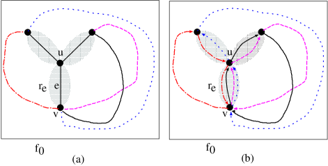
Figure 4: (a) embedding of $\Gamma$ and (b) embedding of $\vec{\Gamma}$.

A search on arc $\vec{e}=(u,v)$ means that we proceed on arc $\vec{e}$ from $u$ to $v$. For each arc $\vec{e}=(u,v)_{\lambda(C)}$, we define its next arc ${\mathop{\rm nx}}(\vec{e})=(v,w)_{\lambda(C)}$ and previous arc ${\mathop{\rm pv}}(\vec{e})=(t,u)_{\lambda(C)}$. For arc $\vec{e}=(u,v)_{\lambda(C)}$, let $C(\vec{e})$ be the oriented cycle that contains $\vec{e}$ and let $L(\vec{e})=\{\vec{h_{1}}={\mathop{\rm nx}}(\vec{e}),..,\vec{h_{t}}\}$, $t\geq 1$, be the set of outgoing arcs from $v$ on the "left side" of $C(\vec{e})$. We assume that arc $\vec{h_{i}}$, $1\leq i\leq t$, in $L(\vec{e})$ is the $i$th outgoing arc from $v$ when we count the arcs incident to $v$ in the counter-clockwise order from ${\mathop{\rm nx}}(\vec{e})$ to $\vec{e}$. We define the leftmost arc from $\vec{e}$, denoted by ${\mathop{\rm lm}}(\vec{e})$, as the $\vec{h_{i}}\in L(\vec{e})$ with the largest $i$ such that ${\mathop{\rm pv}}(\vec{h_{i}})\in{\mathop{\rm ins}}(C(\vec{h_{1}}))\cup\dots\cup{\mathop{\rm ins}}(C(\vec{h}_{i-1}))$ (see Figure 5 for an example). For each arc $\vec{e}=(u,v)_{\lambda(C)}$, ${\mathop{\rm lm}}(\vec{e})$ can be found by checking the arcs in $L(\vec{e})$, starting from ${\mathop{\rm nx}}(\vec{e})$, in the counter-clockwise order they are incident to $v$. A search on a sequence of arcs $\vec{e_{1}},\vec{e_{2}},..$ is called a leftmost search if every $\vec{e}_{i+1}$ is ${\mathop{\rm lm}}(\vec{e_{i}})$ for $i\geq 1$.

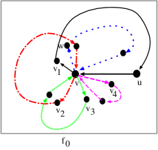
Figure 5: For arc $\vec{e}=(u,v)$, ${\mathop{\rm nx}}(\vec{e})=(v,v_{1})$, $L(\vec{e})=\{(v,v_{1}),(v,v_{2}),(v,v_{3}),(v,v_{4})\}$ and ${\mathop{\rm lm}}(\vec{e})=(v,v_{3})$.

By performing a leftmost search on arcs of $\vec{\Gamma}$, starting from an arbitrary arc in $\vec{E}(f_{0})$, we can find a separating cycle $\vec{C_{m}}$ such that for any cycle $\vec{C}$, $C\in{\cal C}$, if ${\mathop{\rm ins}}(\vec{C_{m}})\cap{\mathop{\rm ins}}(\vec{C})\neq\emptyset$ then ${\mathop{\rm ins}}(\vec{C})\subseteq{\mathop{\rm ins}}(\vec{C_{m}})$. We call $\vec{C_{m}}$ a maximal cycle. According to Lemma 12 and the fact that every cycle $C\in{\cal C}$ has a length at most $k$, the length of $\vec{C_{m}}$ is at most $k$.

After finding $\vec{C_{m}}$, we delete arcs in cycles $\vec{C}$ from $\vec{\Gamma}$ if ${\mathop{\rm ins}}(\vec{C})\subseteq{\mathop{\rm ins}}(\vec{C_{m}})$ to update $\vec{\Gamma}$. We continue the search on the updated $\vec{\Gamma}$ from an arbitrary arc in the updated $\vec{E}(f_{0})$ until all arcs are deleted. Then for each $Z\in{\cal Z}_{X}$, there is a unique maximal cycle which separates $Z$ and $\overline{X}$. For every arc $\vec{e}$ in a maximal cycle $\vec{C_{m}}$, all the arcs in ${\mathop{\rm ins}}(\vec{C_{m}})$ are deleted after $\vec{C_{m}}$ is found. Each arc is counted $O(1)$ time in the computation for all leftmost arc searches. Therefore, the total time complexity of finding all the maximal cycles is $O(m)$.

For each maximal cycle $\vec{C_{m}}$ in $\vec{\Gamma}$ computed above, let $C_{m}$ be the cycle in $H_{X}$ consisting of edges corresponding to the arcs in $\vec{C_{m}}$. For each $Z\in{\cal Z}_{X}$, there is a cycle $C_{m}$ which separates $Z$ and $\overline{X}$. Let $A_{Z}$ be the edge subset induced by $C_{m}$. Then (1) $|\partial(A_{Z})|\leq k$ (if $A_{Z}$ is induced by the boundary cycle $C_{Z}$ then $|\partial(A_{Z})|=|C_{Z}|\leq k$, otherwise $A_{Z}$ is induced by a cycle $C_{m}$ of length at most $k$ as shown in Lemma 11, implying $|\partial(A_{Z})|\leq k$). Due to the way we find the maximal cycles above, (2) for every $Z\in{\cal Z}_{X}$, there is exactly one subset $A_{Z}\in{\mathcal{A}}_{X}$ separating $Z$ and $\overline{X}$; and (3) for distinct $A_{Z},A_{Z^{\prime}}\in{\mathcal{A}}_{X}$, $A_{Z}\cap A_{Z^{\prime}}=\emptyset$. Therefore, ${\mathcal{A}}_{X}$ is a good-separator for ${\cal Z}_{X}$ and $\overline{X}$. $\Box$

We are ready to show Theorem 3 which is re-stated below.

Theorem 5

There is an algorithm which given a planar graph $G$ of $n$ vertices and an integer $k$, in $O(nk^{2})$ time, either constructs a branch-decomposition of $G$ with width at most $(2+\delta)k$ or a $(k+1)\times\lceil{\frac{k+1}{2}}\rceil$ cylinder minor of $G$, where $\delta>0$ is a constant.

Proof:  First, as shown in Lemma 13, a good separator ${\mathcal{A}}_{X}$ for ${\cal Z}_{X}$ and $\overline{X}$ is computed by Subroutine Crest-Separator. From this and as shown in the proof of Theorem 4, given a planar graph $G$ and integer $k$, our algorithm computes a branch-decomposition of $G$ with width at most $(2+\delta)k$ or a $(k+1)\times\lceil{\frac{k+1}{2}}\rceil$ cylinder minor of $G$.

Let $M,m_{x},m$ be the numbers of edges in $G[{\mathop{\rm reach}}_{G|U}(\partial(U),d_{2})],(G|\overline{X})|{\cal Z}_{X},\hat{H}_{X}$, respectively. Then $m=O(m_{x})$. By Lemmas 10 and 13, Subroutine Crest-Separator takes $O(mk^{2})$ time. For distinct level 1 nodes $X$ and $X^{\prime}$, the edge sets of subgraphs $(G|\overline{X})|{\cal Z}_{X}$ and $(G|\overline{X^{\prime}})|{\cal Z}_{X^{\prime}}$ are disjoint. From this, $\sum_{X:\mbox{level 1 node}}m_{x}=O(M)$. Therefore, Step 2 of Procedure Branch-Minor($G|U)$ takes $\sum_{X:\mbox{level 1 node}}O(m_{x}k^{2})=O(Mk^{2})$ time when Steps 2(b)(c) are replaced by Subroutine Crest_Separator.

The time for other steps in Procedure Branch-Minor($G|U$) is $O(M)$. The number of recursive calls in which each vertex of $G|U$ is involved in the computation of Step 2 is $O(\frac{1}{\alpha})=O(1)$. Therefore, we get an algorithm with running time $O(nk^{2})$. $\Box$

5 Concluding remarks

If we modify the definition for $d_{2}$ in Section 3 from $d_{2}=d_{1}+\lceil{\frac{k+1}{2}}\rceil$ to $d_{2}=d_{1}+(k+1)$, we get an algorithm which given a planar graph $G$ and integer $k>0$, in $\min\{O(n\log^{3}n),O(nk^{2})\}$ time either computes a branch-decomposition of $G$ with width at most $(3+\delta)k$, where $\delta>0$ is a constant, or a $(k+1)\times(k+1)$ cylinder minor (or grid minor). It is open whether there is an $O(n)$ time constant factor approximation algorithm for the branchwidth and largest grid (cylinder) minors. The algorithm of this paper can be used to reduce the vertex cut set size in the recursive division of planar graphs with small branchwidth in near linear time. It is interesting to investigate the applications of the algorithm in this paper. Such applications include to improve the efficiency of graph decomposition based algorithms for problems in planar graphs.

References

- [1] S. Arnborg and D. Cornell and A. Proskurowski. Complexity of finding embedding in a k-tree. SIAM J. Disc. Math.8:277–284, 1987.
- [2] S. Arnborg, J. Lagergren, and D. Seese. Easy problems for tree-decomposable graphs. Journal of Algorithms, 12:308–340, 1991.
- [3] Z. Bian, Q.P. Gu. Computing branch decomposition of large planar graphs. In Proc. of the 7th International Workshop on Experimental Algorithms (WEA2008), pages 87-100. 2008.
- [4] Z. Bian, Q.P. Gu, M. Marjan, H. Tamaki and Y. Yoshitake. Empirical Study on Branchwidth and Branch Decomposition of Planar Graphs. In Proc. of the 9th SIAM Workshop on Algorithm Engineering and Experimentation (ALENEX2008), pages 152-165. 2008.
- [5] Z. Bian, Q.P. Gu and M. Zhu. Practical algorithms for branch-decompositions of planar graphs. Discrete Applied Mathematics, doi:10.1016/j.dam.2014.12.017, Jan. 2015.
- [6] H.L. Bodlaender, P.G. Drange, M.S. Dreg, F.V. Fomin, D. Lokshtanov and M. Pilipczuk. An 5-approximation algorithm for treewidth. In Proc. of the 2013 Annual Symposium on Foundation of Computer Science, (FOCS2013), pages 499-508, 2013.
- [7] H.L. Bodlaender. A tourist guide through treewidth. Acta Cybernetica, 11:1–21, 1993.
- [8] H.L. Bodlaender. A linear time algorithm for finding tree-decomposition of small treewidth. SIAM J. Comput. 25:1305–1317, 1996.
- [9] H.L. Bodlaender, A. Grigoriev and A. M. C. A. Koster. Treewidth lower bounds with brambles. Algorithmica. 51(1):81–98, 2008.
- [10] H.L. Bodlaender and D. Thilikos. Constructive linear time algorithm for branchwidth. In Proc. of the 24th International Colloquium on Automata, Languages, and Programming, 627–637, 1997.
- [11] G. Borradaile and D. Eppstein and A. Nayyenri and C. Wulff-Nilsen. All-pairs minimum cuts in near-linear time for surface-embedded graphs. arXiv:1411.7055v1, Nov. 2014.
- [12] G. Borradaile and P. Sankowski and C. Wulff-Nilsen. Min -cut oracle for planar graphs with near-linear preprocessing time. ACM Trans. on Algorithms 11(3), Article 16, Jan. 2015.
- [13] E.D. Demaine and M.T. Hajiaghayi. Graphs excluding a fixed minor have grids as large as treewidth, with combinatorial and algorithmic applications through bidimensionality, In Proc. of the 2005 Symposium on Discrete Algorithms, (SODA 2005), pages 682-689, 2005.
- [14] F. Dorn and F.V. Fomin and M.T. Hajiaghayi and D.M. Thilikos. Subexponential parameterized algorithms on bounded-genus graphs and -minor-free graphs, Jour. of ACM 52(6) pages 866-893, 2005.
- [15] U. Feige, M.T. Hajiaghayi and J.R. Lee. Improved approximation algorithms for minimum weight vertex separators. SIAM J. Comput. 38(2): 629-657, 2008.
- [16] F.V. Fomin and D.M. Thilikos. New upper bounds on the decomposability of planar graphs. Journal of Graph Theory, 51(1):53–81, 2006.
- [17] A. Grigoriev. Tree-width and large grid minors in planar graphs. Discrete Mathematics Theoretical Computer Science. 13(1):13–20, 2011.
- [18] Q.P. Gu and H. Tamaki. Optimal branch decomposition of planar graphs in time. ACM Trans. Algorithms 4(3): article No.30, 1–13, 2008.
- [19] Q.P. Gu and H. Tamaki. Constant-factor approximations of branch-decomposition and largest grid minor of planar graphs in time. Theoretical Computer Science Vol. 412, pages 4100-4109, 2011.
- [20] Q.P. Gu and H. Tamaki. Improved bound on the planar branchwidth with respect to the largest grid minor size. Algorithmica, Vol. 64 pages 416-453, 2012.
- [21] Q.P. Gu and G. Xu. Near-linear time constant-factor approximation algorithm for branch-decomposition of planar graphs. In Proc. of the 40th International Workshop on Graph-Theoretic Concepts in Computer Science, (WG2014), LNCS 8747, pages 238-249, 2014.
- [22] Q.P. Gu and G. Xu. Near-Linear Time Constant-Factor Approximation Algorithm for Branch-Decomposition of Planar Graphs. arXiv:1407.6761v2, March 2015
- [23] I. V. Hicks. Planar branch decompositions I: The ratcatcher. INFORMS Journal on Computing, 17.4 (2005): 402-412.
- [24] I. V. Hicks. Planar branch decompositions II: The cycle method. INFORMS Journal on Computing, 17.4 (2005): 413-421.
- [25] F. Kammer. Treelike and Chordal Graphs: Algo- rithms and Generalizations.. PhD thesis, 2010.
- [26] F. Kammer and T. Tholey. Approximate tree decompositions of planar graphs in linear time. In Proc. of the 2012 Annual ACM-SIAM Symposium on Discrete Algorithms (SODA2012), pages 683–698, 2012.
- [27] F. Kammer and T. Tholey. Approximate tree decompositions of planar graphs in linear time. arXiv:1104.2275v2, May 2013
- [28] F. Kammer and T. Tholey. Approximate tree decompositions of planar graphs in linear time. arXiv:1104.2275v3, July 2015
- [29] S. Mozes and C. Sommer. Exact distance oracles for planar graphs In Proc. of the 2012 Annual ACM-SIAM Symposium on Discrete Algorithms, (SODA 2012), pages 209-222, 2012.
- [30] J.H. Reif. Minimum s-t cut of a planar undirected network in time. planar graphs in linear time. SIAM J. on Computing, 12(1): pages 71-81, 1983
- [31] N. Robertson and P.D. Seymour. Graph minors X. Obstructions to tree decomposition. J. of Combinatorial Theory, Series B, 52:153–190, 1991.
- [32] N. Robertson and P.D. Seymour. Graph minors XIII. The disjoint paths problem. of Combinatorial Theory, Series B, 63:65–110, 1995.
- [33] N. Robertson and P.D. Seymour and R. Thomas. Quickly excluding a planar graph J. of Combinatorial Theory, Series B, 62:323–348, 1994.
- [34] P.D. Seymour and R. Thomas. Call routing and the ratcatcher. Combinatorica, 14(2):217–241, 1994.
- [35] J. C. Smith, E. Ulusal, and I. V. Hicks. A combinatorial optimization algorithm for solving the branchwidth problem. Computational Optimization and Applications, 51.3 (2012): 1211-1229.
- [36] H. Tamaki. A linear time heuristic for the branch-decomposition of planar graphs. In Proc. of ESA2003 765–775, 2003.
- [37] M. Thorup. Undirected single-source shortest paths with positive integer weights in linear time. Journal of the ACM, 46(3):362–394, 1999.
- [38] K. Ton, C. Lee, and J. Liu. New algorithms for k-face cover, k-feedback vertex set, and k-disjoint cycles on plane and planar graphs. In Graph-Theoretic Concepts In Computer Science, (WG2002), pages 282-295, 2002.