Stochastic six-vertex model

Abstract.

We study the asymmetric six-vertex model in the quadrant with parameters on the stochastic line. We show that the random height function of the model converges to an explicit deterministic limit shape as the mesh size tends to $0$. We further prove that the one-point fluctuations around the limit shape are asymptotically governed by the GUE Tracy–Widom distribution. We also explain an equivalent formulation of our model as an interacting particle system, which can be viewed as a discrete time generalization of ASEP started from the step initial condition. Our results confirm an earlier prediction of Gwa and Spohn (1992) that this system belongs to the KPZ universality class.

1. Introduction

In this article we study a stochastic system at the interface of equilibrium lattice models and non-equilibrium interacting particle systems.

From the point of view of lattice models, we deal with the six–vertex (or “square–ice”) model. The configurations of the six–vertex model are assignments of one of 6 types of $H_{2}O$ molecules shown in Figure 1 to the vertices of (a subdomain of) square grid in such a way that the $O$ atoms are at the vertices of the grid. To each $O$ atom there are two $H$ atoms attached, so that they are at angles $90^{\circ}$ or $180^{\circ}$ to each other, along the grid lines, and between any two adjacent $O$ atoms there is exactly one $H$. Figure 2 shows an example of a configuration.

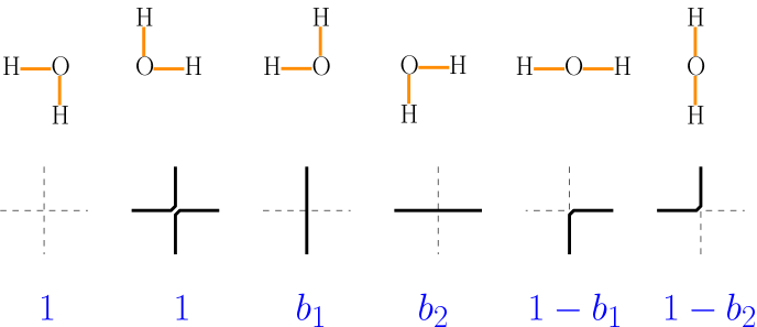
Figure 1. Six types of vertices in $H_{2}O$ interpretation (top panel) and in lines interpretation (middle panel). Weights corresponding to the vertices for measure $\mathcal{P}(b_{1},b_{2})$ (bottom panel).

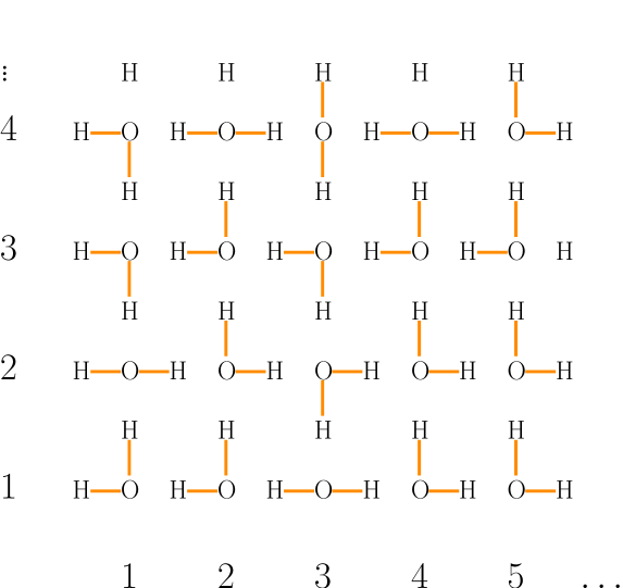
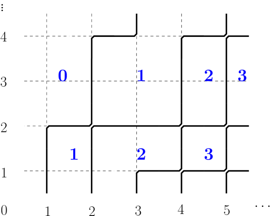
Figure 2. Part of the configuration of the model in quadrant (left panel), corresponding line ensemble and height function (right panel).

The six–vertex model is an important model of equilibrium statistical mechanics, being the prototypical integrable lattice model in two dimensions. Its study has led to many exciting developments during the last 50 years, see e.g. [Bax], [Resh] and references therein. Our interest is probabilistic: we study random configurations and the asymptotic distributions of the quantities describing them.

In the present paper we are concerned with the model in a quadrant, i.e. on the grid $\mathbb{Z}_{>0}\times\mathbb{Z}_{>0}$, and with specific boundary conditions: $H$ atoms on the left boundary and alternating $H$ and $O$ atoms on the bottom boundary, as shown in Figure 2. Such boundary conditions can be viewed as an infinite analogue of the well-studied domain–wall boundary conditions, cf. [Br], [Z], [Gi], [BFZ, Introduction] for reviews of many recent results about the latter.

There is no canonical (e.g. uniform) measure on the configurations in the quadrant. Informally, we are working with a special class of the asymmetric six-vertex models whose parameters fall on what is sometimes called the stochastic line, cf. [GS], [ADW], [Ki], [PS2]. More formally, we introduce and study the family of measures $\mathcal{P}(b_{1},b_{2})$ depending on two parameters $0<b_{1}<1$ and $0<b_{2}<1$. The measure $\mathcal{P}(b_{1},b_{2})$ can be defined through the following stochastic sampling algorithm. The types of vertices of $\mathcal{P}(b_{1},b_{2})$–random configuration $\omega$ are chosen sequentially: we start from the corner vertex at $(1,1)$, then proceed to $(1,2)$ and $(2,1)$,…, then proceed to all vertices $(x,y)$ with $x+y=k$, then with $x+y=k+1$, etc. The combinatorics of the model implies that when we choose the type of the vertex $(x,y)$, then either it is uniquely determined by the types of its previously chosen neighbors, or we need to choose between vertices of types number $3$ and number $5$ at Figure 1, or we need to choose between vertices of types $4$ and $6$. We do all the choices independently and choose type $3$ with probability $b_{1}$ and type $5$ with probability $1-b_{1}$. Similarly we choose type $4$ with probability $b_{2}$ and type $6$ with probability $1-b_{2}$. All these probabilities are recorded in Figure 2 and we refer to Section 2.1 for a more detailed description of $\mathcal{P}(b_{1},b_{2})$.

Alternatively, the measure $\mathcal{P}(b_{1},b_{2})$ can be obtained as a limit of Gibbs measures in certain finite domains approximating the quadrant, see Section 2.1 for the exact statement. Furthermore, below and also in Section 2.2 we explain that $\mathcal{P}(b_{1},b_{2})$–random configurations can be identified with time evolution of a certain interacting particle system.

In order to state our results we need to introduce the height function of a model configuration. For that we use a known identification of the six–vertex model with an ensemble of paths, which is obtained by replacing the 6 types of $H_{2}O$ molecules with corresponding $6$ types of local line configurations as shown in Figure 1. The result is an ensemble of paths in the quadrant: all paths start at the bottom boundary and follow the up–right directions, corners of the paths are allowed to touch, but paths never intersect each other, see Figure 2 for an example. These paths can be viewed as level lines of a certain function. More precisely, for a configuration $\omega$ we define its height function $H(x,y;\omega)$, $x,y\in\mathbb{R}_{>0}$, (here $x$ is the horizontal coordinate) by setting $H(0,y;\omega)=0$ and declaring that when we cross a path, $H(x,y;\omega)$ increases by $1$, as shown in Figure 2. A formal way of doing that is to define $H(x,y;\omega)$ as the number of vertices of types $2$, $3$ and $5$ (non-strictly) to the left from point $(x,\lceil y\rceil)$.

Our first result is the Law of Large Numbers for the height function.

Theorem 1.1.

Assume that $0<b_{2}<b_{1}<1$ and let $\omega$ be a $\mathcal{P}(b_{1},b_{2})$–distributed random configuration. Then for any $x,y>0$ the following convergence in probability holds

$$\lim_{L\to+\infty}\frac{H(Lx,Ly;\omega)}{L}=\mathcal{H}(x,y),$$

where

$$\mathcal{H}(x,y)=\begin{dcases}\dfrac{\left(\sqrt{y(1-b_{1})}-\sqrt{x(1-b_{2})}\right)^{2}}{b_{1}-b_{2}},&\dfrac{1-b_{1}}{1-b_{2}}<\dfrac{x}{y}<\dfrac{1-b_{2}}{1-b_{1}},\\ 0,&\dfrac{x}{y}\leq\dfrac{1-b_{1}}{1-b_{2}},\\ x-y,&\dfrac{x}{y}\geq\dfrac{1-b_{2}}{1-b_{1}}.\end{dcases}$$

We remark that for the six–vertex model in a finite (but growing) domain with fixed boundary conditions, there is a general approach to the laws of large numbers similar to Theorem 1.1 through the associated variational problem, as is briefly outlined in [PR]. However, as far as the authors know, mathematically the variational approach has not been yet developed to the point where it could produce a rigorous proof of Theorem 1.1; we use completely different methods to prove this theorem. Note that in a related context of random height function arising from tilings and dimer models, the variational approach is much more developed, see [CKP], [KOS], [KO]. We will revisit the idea of variational problems later from a point of view of interacting particle systems.

Our next result identifies the asymptotic fluctuations of the height function. Observe that the limit shape $\mathcal{H}(x,y)$ is curved in the sector $\frac{1-b_{1}}{1-b_{2}}<\frac{x}{y}<\frac{1-b_{2}}{1-b_{2}}$ and flat outside it (as $b_{1}\to b_{2}$ the curved region disappears). The regions where $\mathcal{H}(x,y)$ is flat are typically called frozen regions, and one expects the fluctuations to be exponentially small there. In the curved (also called “liquid”) region the situation is different.

Theorem 1.2.

Assume that $0<b_{2}<b_{1}<1$ and let $\omega$ be $\mathcal{P}(b_{1},b_{2})$–distributed random configuration. For any $x,y$ such that $\frac{1-b_{1}}{1-b_{2}}<\frac{x}{y}<\frac{1-b_{2}}{1-b_{2}}$, and any $s\in\mathbb{R}$ we have

$$\lim_{L\to\infty}\mathbb{P}\left(\frac{\mathcal{H}(x,y)L-H(Lx,Ly;\omega)}{\sigma_{x,y}L^{1/3}}\leq s\right)=F_{{\rm GUE}}(s),$$

where

$$\sigma_{x,y}=\kappa^{-1/3}\frac{x^{1/6}y^{1/6}}{\kappa^{-1/2}-\kappa^{1/2}}\left(1-\sqrt{\kappa x/y}\right)^{2/3}\left(1-\sqrt{\kappa y/x}\right)^{2/3},\quad\quad\kappa=\frac{1-b_{1}}{1-b_{2}},$$ (1)

and $F_{{\rm GUE}}$ is the GUE Tracy-Widom distribution.

Remark. The symmetry $\sigma_{x,y}=\sigma_{y,x}$ can be traced to the fact that the measures $\mathcal{P}(b_{1},b_{2})$ are invariant under the involution which reflects the configuration by the $x=y$ line and then swaps the types of vertices in pairs $1\leftrightarrow 2$, $3\leftrightarrow 4$, $5\leftrightarrow 6$. Another feature of (1) is that if we formally replace $\kappa$ by $\kappa^{-1}$ in the formula, then $\sigma_{x,y}$ changes its sign; we do not have any good explanations for the latter property.

We recall that $F_{{\rm GUE}}$ is the limiting distribution for the largest eigenvalue of the random Hermitian matrices (as the size of the matrix tends to infinity) from the Gaussian Unitary Ensemble, see [TW1]. One way to compute the distribution function $F_{{\rm GUE}}(s)$ is through the Fredholm determinant expression:

$$F_{{\rm GUE}}(s)=\det(I-A)_{L_{2}(s,+\infty)},$$

where $A$ is an integral operator on $L_{2}(s,+\infty)$ with kernel expressed though the Airy function via

$$A(x,y)=\frac{Ai(x)Ai^{\prime}(y)-Ai(y)Ai^{\prime}(x)}{x-y}.$$

Theorem 1.2 is not the first instance of the appearance of a distribution of the random matrix origin in the asymptotics of the six–vertex model. There is a class of measures on configurations of the six–vertex model, called the free fermion point of the model, which can be analyzed via techniques of determinantal point processes. In particular, for the six–vertex model in $N\times N$ square with domain–wall boundary conditions the study of these free fermion models is the same as the study of random domino tilings of the Aztec diamond, see [EKLP], [Ku], [FS1] for the details. Uniformly random tilings of the Aztec diamond are known to posses random matrix asymptotic behavior, see [J3], [JN]. However, we do not know any direct relation of our measures $\mathcal{P}(b_{1},b_{2})$ with free fermion point or determinantal point processes. Outside free fermions, the only connection to random matrices that we are aware of, is the results of [GP],[G] for the six–vertex model with domain–wall boundary conditions.

While the appearance of the random matrix type distribution in the six–vertex model is anticipated, the exact form of Theorem 1.2 is a bit unexpected from the point of view of statistical mechanics models with height functions. Indeed, in many related models the asymptotic fluctuations of the height function are Gaussian and, more precisely, are governed by the Gaussian Free Field, cf. [Ken], [BF2], [P], [Bor], [BG]. Theorem 1.2 can probably be better understood from the point of view of interacting particle systems which we now present.

The connection of the six–vertex model to an interacting particle system with local interactions was first noticed in [GS]. In order to see it in our context, we need to break the symmetry between $x$ and $y$ coordinates. Consider $\mathcal{P}(b_{1},b_{2})$–distributed random configuration and cut it by horizontal lines $y=t+1/2$, $t=0,1,2,\dots$ as shown in Figure 3. The intersection of the horizontals with bold lines of the configurations (that is, level lines of the height function) produce particle configuration $\mathbf{X}^{b_{1},b_{2}}(t)=(x_{1}(t)<x_{2}(t)<\dots)$.

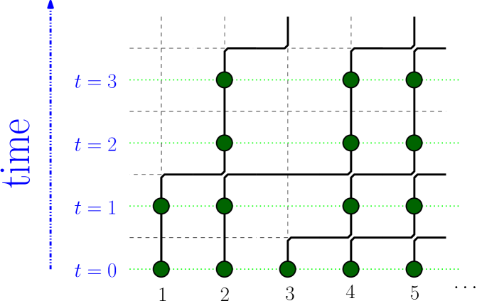
Figure 3. $5\times 4$ part of a configuration of the six–vertex model in the quadrant and corresponding particle system.

The definition of the measure $\mathcal{P}(b_{1},b_{2})$ readily implies that $\mathbf{X}^{b_{1},b_{2}}(t)$, $t=0,1,\dots$, is a Markov chain. Moreover, this Markov chain has local update rules, as we explain in more details in Section 2.2.

From the point of view of $\mathbf{X}^{b_{1},b_{2}}(t)$, Theorem 1.1 becomes the law of large numbers for the large time current of an interacting particle system. Thus, this result may also be derivable through hydrodynamic theory as the solution to a one-dimensional variational problem (cf. [Spo1], [Ro], [Se], [Rez], [Spo2]) or as the solution to a Hamilton-Jacobi PDE with flux which was computed in [GS]. The curved or liquid part of the limit shape $\mathcal{H}(x,y)$ in the interacting particle systems language is known as the rarefaction fan. Further, the features of Theorem 1.2, i.e. the scaling exponent $L^{1/3}$ and the appearance of $F_{GUE}$ are a manifestation of the fact that $\mathbf{X}^{b_{1},b_{2}}(t)$ belongs to the KPZ universality class, see [Cor1] for a recent review of KPZ universality. Note that the $L^{1/3}$ exponent was first predicted in this model by [GS] based on the computation of the mixing time for the same interacting particle system on a cylinder. Both $L^{1/3}$ exponent and the limiting distribution $F_{GUE}$ were found before in several other interacting particle systems starting from the work [J1] on the Totally Asymmetric Simple Exclusion Process (TASEP). The latter (as well as other systems, see [FS2] for a survey) can be analyzed essentially using the techniques of determinantal point processes. More recently and using a somewhat different set of techniques, similar results were obtained for more complicated systems including Asymmetric Simple Exclusion Process (ASEP) [TW4], [BCS], $q$–TASEP [BC], [FV], and the solution to KPZ stochastic partial differential equation [ACQ], [SS], [D], [CDR], [BCF]; see also [BG2], [BP], [Cor3] for reviews.

The process $\mathbf{X}^{b_{1},b_{2}}(t)$ has a limit to ASEP when $b_{1}\to 0$ with $b_{2}/b_{1}$ fixed, see Section 2.2 for more details. Further limits include TASEP ($b_{2}=0$, $b_{1}\to 0$) and KPZ stochastic partial differential equation (see [KPZ], [BeGi], [ACQ]).

The relation to the KPZ universality class leads to predictions on multipoint fluctuations of the height function $H(x,y;\omega)$. For instance, we expect (but the proof is out of reach with our present techniques) that if we fix $x,y$ satisfying $\frac{1-b_{1}}{1-b_{2}}<\frac{x}{y}<\frac{1-b_{2}}{1-b_{2}}$, and vary $\zeta\in\mathbb{R}$, then the (proper centered and scaled) random process $H(Lx+L^{2/3}\zeta,Ly;\omega)$ converges in distribution to the Airy₂ process (i.e. the top line of the Airy line ensemble). We refer to [PS2],[J2],[J3],[BF1] for similar statements for the interacting particle systems related to the determinantal point processes.

The techniques we use to prove Theorems 1.1 and 1.2 also rely on the interacting particle system interpretation. We start by finding the eigenfunctions of the matrix of transitional probabilities of $\mathbf{X}^{b_{1},b_{2}}(t)$ (when there are only finitely many particles). Similar computations go back to the seminal work [L] on the six–vertex model in 60s. The eigenrelation leads to contour integral formulas for the transitional probabilities of $\mathbf{X}^{b_{1},b_{2}}(t)$ which turns out to be very similar to those of the ASEP. This allows us to use techniques developed in [TW2] to find certain marginals of the distribution of $\mathbf{X}^{b_{1},b_{2}}(t)$. We further manipulate these expressions and use techniques developed in [BC], [BCS] (for the analysis of $q$–TASEP and certain directed polymers) to obtain a Fredholm determinant formula for the $q$–Laplace transform of one-point distribution for the height function $H(x,y;\omega)$. A steepest descent analysis of the kernel for this Fredholm determinant ultimately leads to the results of Theorems 1.1 and 1.2.

Acknowledgements. We would like to thank H. Spohn for useful discussions. A.B. was partially supported by the NSF grant DMS-1056390. I.C. was partially supported by the NSF through DMS-1208998 as well as by Microsoft Research and MIT through the Schramm Memorial Fellowship, by the Clay Mathematics Institute through the Clay Research Fellowship, and by the Institute Henri Poincare through the Poincare Chair. V. G. was partially supported by the NSF grant DMS-1407562.

2. Two formulations of the model

Let us start by giving a formal definition of our main subject of study — the measure $\mathcal{P}(b_{1},b_{2})$. For convenience we stick to the bold lines interpretation of the six–vertex model, the $H_{2}O$ molecules picture can be always restored through the bijection of Figure 1.

The configuration of the model is an assignment of the pictures of 6 kinds shown in Figure 4 to the vertices of the grid $\mathbb{Z}_{>0}\times\mathbb{Z}_{>0}$ subject to three restrictions:

Figure 4. Six types of vertices, corresponding lines and weights.

• The pictures at any two adjacent sites agree in the sense that the bold lines keep flowing. E.g. if a picture at position $(x,y)$ has a bold line in west direction, then the picture at position $(x-1,y)$ should have a bold line in east direction.

• Pictures at positions $(x,1)$ for $x>0$ have bold lines in south direction.

• Pictures at positions $(1,y)$ for $y>0$ do not have bold lines in west direction.

Let $\Omega$ denote the space of all configurations satisfying the above conditions. One element from $\Omega$ is shown in the right panel of Figure 2. We remark that traditionally, one subdivides the six–types into $3$ pairs $a_{1}$, $a_{2}$, $b_{1}$, $b_{2}$, $c_{1}$, $c_{2}$, as shown in Figure 4, and we use such notation for the types of vertices.

We now explain a procedure for sampling a $\mathcal{P}(b_{1},b_{2})$–distributed element $\omega\in\Omega$, thus defining the measure.

Let $\omega(x,y)$ denote the type of the vertex at $(x,y)$ and proceed inductively in $x+y$, i.e. we first sample the vertices with $x+y=2$, then with $x+y=3$, etc. When we sample $\omega(x,y)$, the vertices $\omega(x-1,y)$ and $\omega(x,y-1)$ are already known, therefore, we know whether the south and west lines in $\omega(x,y)$ should be bold or not. Thus, we have four cases:

• If both west and south lines in $\omega(x,y)$ are bold, then we set $\omega(x,y)$ to be of type $a_{2}$.

• If both west and south lines in $\omega(x,y)$ are not bold, then we set $\omega(x,y)$ to be of type $a_{1}$.

• If the west line in $\omega(x,y)$ is bold, while the south line in $\omega(x,y)$ is not bold, then we set $\omega(x,y)$ to be of type $b_{2}$ with probability $b_{2}$ and to be of type $c_{2}$ with probability $1-b_{2}$.

• If the west line in $\omega(x,y)$ is not bold, while the south line in $\omega(x,y)$ is bold, then we set $\omega(x,y)$ to be of type $b_{1}$ with probability $b_{1}$ and to be of type $c_{1}$ with probability $1-b_{1}$.

Definition 2.1.

$\mathcal{P}(b_{1},b_{2})$ is the probability measure on $\Omega$ obtained by the above sampling procedure.

The measures $\mathcal{P}(b_{1},b_{2})$ can be put into two different contexts. In Section 2.1 we explain that these measures are specific Gibbs measures for the six–vertex model with a quadratic relation on weights of the vertices $a_{1},a_{2},b_{1},b_{2},c_{1},c_{2}$. In Section 2.2 we explain that $\mathcal{P}(b_{1},b_{2})$ can be viewed as the law of an interacting particle system.

2.1. $\mathcal{P}(b_{1},b_{2})$ as a Gibbs measure for the six–vertex model

We want to study probability measures on $\Omega$ satisfying the Gibbs property encoded by $6$ positive weights $a_{1},a_{2}$, $b_{1},b_{2}$, $c_{1},c_{2}$. The identification of weights and types of vertices is shown in Figure 4 and somewhat abusing the notations we will use the same notation for them; e.g. we write $a_{1}$ both for the type of a vertex and for the corresponding positive weight.

Definition 2.2.

A probability measure $P$ on $\Omega$ is called Gibbs, if for any finite subdomain $S\subset\mathbb{Z}_{>0}\times\mathbb{Z}_{>0}$, the conditional distribution of $P$ on the configurations inside $S$ given the configuration outside $S$ has weights proportional to

$$(a_{1})^{\#(a_{1})}(a_{2})^{\#(a_{2})}(b_{1})^{\#(b_{1})}(b_{2})^{\#(b_{2})}(c_{1})^{\#(c_{1})}(c_{2})^{\#(c_{2})},$$

where $\#(a_{1})$ means the number of vertices of type $a_{1}$ inside $S$ and similarly for other types.

We are not aware of any classification theorems for the Gibbs measures on $\Omega$. However, we note that in related contexts theorems of this kind are known (cf. [Sh], [GH], [G1]).

We will obtain our Gibbs measures as limits of the Gibbs measures on growing finite subdomains of $\Omega$.

For two positive integers $X$ and $Y$ let $\Omega(X,Y)$ denote the set of the configurations of the six–vertex model in $\{1,\dots,X\}\times\{1,\dots,Y\}$ satisfying the same boundary condition as configurations from $\Omega$ along the south and west boundaries and no boundary conditions along the north and east boundaries. For instance, the right panel of Figure 2 can be viewed as a configuration from $\Omega(5,4)$. There are finitely many configurations in $\Omega(X,Y)$ and we equip $\Omega(X,Y)$ with a Gibbs probability measure $P(X,Y;a_{1},a_{2},b_{1},b_{2},c_{1},c_{2})$ such that the probability of $\omega\in\Omega(X,Y)$ having $\#(a_{1})$ vertices of type $a_{1}$, $\#(a_{2})$ vertices of type $a_{2}$, etc., is

$$\frac{(a_{1})^{\#(a_{1})}(a_{2})^{\#(a_{2})}(b_{1})^{\#(b_{1})}(b_{2})^{\#(b_{2})}(c_{1})^{\#(c_{1})}(c_{2})^{\#(c_{2})}}{Z(X,Y;a_{1},a_{2},b_{1},b_{2},c_{1},c_{2})},$$

where $Z(\cdot)$ is a normalization constant.

Clearly, $\Omega$ can be viewed as an a limit of $\Omega(X,Y)$ as $X,Y\to\infty$. We say that a probability measure $M$ is a limit of measures $M_{n}$ on $\Omega(X_{n},Y_{n})$ as $n\to\infty$ if $\lim_{n\to\infty}X_{n}=\lim_{n\to\infty}Y_{n}=\infty$ and for any finite collection $(x_{1},y_{1})$, …$(x_{k},y_{k})$ and for any set of types $t_{i}\in\{a_{1},a_{2},b_{1},b_{2},c_{1},c_{2}\}$, $i=1,\dots,k$, the $M$–probability of having the vertices of types $t_{1}$, …, $t_{k}$ in positions $(x_{1},y_{1})$, …, $(x_{k},y_{k})$ is the $n\to\infty$ limit of the $M_{n}$–probabilities for the same event. We similarly define taking limits as only one of $X_{n}$, $Y_{n}$ tends to infinity, or if one of $X$ and $Y$ is already infinite.

Proposition 2.3.

1. Suppose that the weights of the six–vertex model satisfy the quadratic relation

   $$c_{1}c_{2}=(a_{1}-b_{2})(a_{2}-b_{1}),$$ (2)

   and inequality $a_{1}>b_{2}$, which guarantees that the factors in (2) are positive. Then the measure $\mathcal{P}$ (from Definition 2.1) can be obtained through the following iterated limit:

   $$\mathcal{P}\left(\frac{b_{1}}{a_{2}},\frac{b_{2}}{a_{1}}\right)=\lim_{Y\to\infty}\lim_{X\to\infty}P(X,Y;a_{1},a_{2},b_{1},b_{2},c_{1},c_{2}),$$ (3)

   where the limits are understood as explained above.

2. Suppose that the weights of the six–vertex model satisfy the quadratic relation

   $$c_{1}c_{2}=(a_{1}-b_{1})(a_{2}-b_{2}),$$ (4)

   and inequality $a_{1}>b_{1}$, which guarantees that the factors in (4) are positive. Then the measures $\mathcal{P}$ (from Definition 2.1) can be obtained through the following iterated limit:

   $$\mathcal{P}\left(\frac{b_{1}}{a_{1}},\frac{b_{2}}{a_{2}}\right)=\lim_{X\to\infty}\lim_{Y\to\infty}P(X,Y;a_{1},a_{2},b_{1},b_{2},c_{1},c_{2}).$$ (5)

Remark 1. It is very plausible that the limits in (3), (5) exist also when the conditions (2), (4) are not satisfied, and, even further, when instead of iterative limit, we send $X$ and $Y$ to $\infty$ simultaneously in certain regular ways. However, the limiting measures would probably be different from the family $\mathcal{P}(b_{1},b_{2})$ and we do not analyze such limits of measures in the present article.

Remark 2. The quadratic relation (2) was introduced in [GS]. Under this condition the transfer matrix (see Section 3) can be easily renormalized to become stochastic (and related to interacting particle systems described in Section 2.2).

Proof of Proposition 2.3.

We first analyze $\lim_{Y\to\infty}\lim_{X\to\infty}P(X,Y;a_{1},a_{2},b_{1},b_{2},c_{1},c_{2})$ under condition (2).

Take a fixed finite $Y$ and large $X$ and consider the $P(X,Y;a_{1},a_{2},b_{1},b_{2},c_{1},c_{2})$–distributed configuration $\omega$. Note that our boundary condition implies that in the horizontal row $y$ there are at most $y$ vertices of types $a_{1}$, $b_{2}$, $c_{1}$, $c_{2}$ and all others are either of type $a_{2}$ or $b_{1}$. Furthermore, the vertices of types $a_{2}$ and $b_{1}$ clearly cannot be horizontally adjacent. Together with the inequality $a_{2}>b_{1}$ this implies that with probability tending to $1$ as $X\to\infty$ all the vertices in the vertical column $X$ are of type $a_{2}$. As a conclusion, tracing the paths which start at the bottom boundary, we see that with probability tending to $1$ the total number of the vertices of types $a_{2}$, $b_{1}$ and $c_{1}$ is equal to $XY-(1+2+\dots+Y)$. In particular, this number becomes deterministic. Since the number of all vertices is always $XY$, the total number of the vertices of types $a_{1}$, $b_{2}$ and $c_{2}$ also becomes deterministic.

In addition, looking at horizontal bold lines, we see that in each horizontal row $y$, the number of the vertices of type $c_{1}$ is $1$ plus the number of the vertices of type $c_{2}$. Therefore, the difference between the total number of the vertices of types $c_{1}$ and $c_{2}$ also becomes deterministic.

The argument of the previous two paragraph implies now that if we multiply the weights $a_{2}$, $b_{1}$ and $c_{1}$ by a constant $U$, the weights $a_{1}$, $b_{2}$ and $c_{2}$ by another constant $V$, the weight $c_{1}$ by another constant $W$ and the weight $c_{2}$ by $1/W$, then the limit $\lim_{X\to\infty}P(X,Y;a_{1},a_{2},b_{1},b_{2},c_{1},c_{2})$ will not change. Choosing appropriate constants $U=\frac{1}{a_{2}}$, $V=\frac{1}{a_{1}}$, $W=\frac{1-b_{1}/a_{2}}{c_{1}/a_{2}}$, taking into the account (2) and adapting the notations $\tilde{b}_{1}=b_{1}/a_{2}$, $\tilde{b}_{2}=b_{2}/a_{1}$, we can transform the six weights $(a_{1},a_{2},b_{1},b_{2},c_{1},c_{2})$ into new six weights $(1,1,\tilde{b}_{1},\tilde{b}_{2},1-\tilde{b}_{1},1-\tilde{b}_{2})$. Under new weights we immediately see the convergence to the above description for sampling $\mathcal{P}(\tilde{b}_{1},\tilde{b}_{2})$ (in fact, for the new parameters the same algorithm works for any finite domain $\Omega(X,Y)$).

In order to analyze the limit in the different order $\lim_{X\to\infty}\lim_{Y\to\infty}P(X,Y;a_{1},a_{2},b_{1},b_{2},c_{1},c_{2})$, note that $\Omega$ possesses the following involutive symmetry: take a configuration $\omega\in\Omega$, reflect it by the main diagonal $x=y$ and further interchange the bold and dotted lines of Figure 4. As a result we obtain another configuration from $\Omega$. Note that under this transformation, the vertices of types $b_{1}$, $b_{2}$, $c_{1}$, $c_{2}$ turn into the vertices of the same type (in reflected positions), while the vertices of types $a_{1}$ and $a_{2}$ swap their types. Hence, (4) and (5) are obtained from (2) and (3) by this involution. ∎

2.2. $\mathcal{P}(b_{1},b_{2})$ as an interacting particle system

It was observed in [GS] that under the quadratic condition (2) the six–vertex model can be naturally related to a certain interacting particle system. Let us describe how this works for our measures $\mathcal{P}(b_{1},b_{2})$.

Consider $\mathcal{P}(b_{1},b_{2})$–distributed random configuration and cut it by horizontal lines $y=t+1/2$, $t=0,1,2,\dots$ as shown in Figure 3. The intersection of the horizontals with bold lines produces particle configuration $\mathbf{X}^{b_{1},b_{2}}(t)=(x_{1}(t)<x_{2}(t)<\dots)$.

The definition of the measure $\mathcal{P}(b_{1},b_{2})$ via a local sampling procedure readily implies that $\mathbf{X}^{b_{1},b_{2}}(t)$, $t=0,1,\dots$ is a Markov chain and moreover can be viewed as an interacting particle system with local interactions. Indeed, given $\mathbf{X}^{b_{1},b_{2}}(t)$, the configuration $\mathbf{X}^{b_{1},b_{2}}(t+1)$ can be defined as follows: we sequentially define the positions $x_{i}(t+1)$ of the particles for $i=1,2,\dots$. The $i$th particle at position $x_{i}(t)$ jumps at time $t+1$ to any position from the interval $\{\max(x_{i-1}(t+1)+1,x_{i}(t)),\max(x_{i-1}(t+1)+1,x_{i}(t))+1,\dots,x_{i+1}(t)\}$ with the following probabilities:

• If $x_{i-1}(t+1)\leq x_{i}(t)$, then

  $$\mathbb{P}\biggl{(}x_{i}(t+1)=x_{i}(t)+k\mid\mathbf{X}^{b_{1},b_{2}}(t),x_{i-1}(t+1)\biggr{)}\\ =\begin{cases}b_{1},&k=0,\\ (1-b_{1})(1-b_{2})b_{2}^{k-1},&0<k<x_{i+1}(t)-x_{i}(t),\\ (1-b_{1})b_{2}^{x_{i+1}(t)-x_{i}(t)-1},&k=x_{i+1}(t)-x_{i}(t),\\ 0,&\text{otherwise.}\end{cases}$$

• If $x_{i-1}(t+1)=x_{i}(t)$, then

  $$\mathbb{P}\biggl{(}x_{i}(t+1)=x_{i}(t)+k\mid\mathbf{X}(t),x_{i-1}(t+1)\biggr{)}=\begin{cases}(1-b_{2})b_{2}^{k-1},&0<k<x_{i+1}(t)-x_{i}(t),\\ b_{2}^{x_{i+1}(t)-x_{i}(t)-1},&k=x_{i+1}(t)-x_{i}(t),\\ 0,&\text{otherwise.}\end{cases}$$

Informally, one says that the $i$th particle flips a $b_{1}$–biased coin to decide whether it stays on its position, or not. If not, then it jumps to the right with $b_{2}$–geometric probabilities; when it reaches the $i+1$st particle, it can push it to the right, but at most by $1$. After that the $i+1$st particle starts to move, etc.

The definition implies that $\mathbf{X}^{b_{1},b_{2}}(0)=(1,2,3,\dots)$, such configuration at time $0$ is usually referred to as step initial condition. Note that the state space of the Markov chain $\mathbf{X}^{b_{1},b_{2}}(t)$ is countable, which is a consequence of the choice of the initial condition, see Section 3.2 for more details.

There is a connection of our interacting particle system to the Asymmetric Simple Exclusion Process (ASEP). Recall that ASEP is an interacting particle system on $\mathbb{Z}$ in continuous time in which each particle has two (exponential) clocks: the right clock of intensity $p$ and the left clock of intensity $q$. When the right clock rings the particle checks whether the position to its right is free: if Yes, then it jump by $1$ to the right, if No, then nothing happens. When the left clock rings the particle checks whether the position to its left is free: if Yes, then it jump by $1$ to the left, if No, then nothing happens. Afterwards the clocks are restarted. The ASEP is a very well studied model, cf. [Spi], [Lig1], [Lig2], [TW4], [Cor2].

We are not going to provide the proof, but it is very plausible that the following is true: for any two reals $p,q>0$

$$\lim_{\varepsilon\to 0}\mathbf{X}^{\varepsilon q,\varepsilon p}(\lfloor\varepsilon^{-1}t\rfloor)-\varepsilon^{-1}t=\mathbf{Y}^{p,q}(t),$$ (6)

where $\mathbf{Y}^{p,q}(t)$ is ASEP started with step initial condition, i.e. $\mathbf{Y}^{p,q}(0)=(1,2,3,\dots)$. It is important to emphasize the subtraction of $\varepsilon^{-1}t$ in (6). In other words, we observe ASEP near the diagonal. Note that for $k$–particle version of $\mathbf{X}^{b_{1},b_{2}}(t)$ an analogue of (6) is straightforward, moreover, it will be clear below (see Theorem 3.6 and remark after it) that the formulas we get for the transitional probabilities of the $k$–particle version of $\mathbf{X}^{b_{1},b_{2}}(t)$ converge to those for $k$–particle ASEP. However, in order to rigorously prove (6) one would need to deal with infinitely many particles which we leave out of the scope of the present article.

Another curious limit is obtained if we send $b_{1}\to 1$ (we again do not provide a complete proof). Set

$$\mathbf{Z}^{b}(t)=\lim_{\varepsilon\to 0}\mathbf{X}^{\varepsilon^{-1},b}(\lfloor\varepsilon^{-1}t\rfloor).$$ (7)

The dynamics $\mathbf{Z}^{b}(t)$ has the following description: each particle has an independent exponential clock of rate $1$. When the clock of $i$th particle rings at time $t$, it wakes up and jumps to the right by $k$ steps $(0<k<x_{i+1}(t)-x_{i}(t))$ with probability $(1-b)b^{k-1}$. With remaining probability $b^{x_{i+1}(t)-x_{i}(t)-1}$ the $i$th particle jumps to the position of $x_{i+1}(t)$ of the $(i+1)$st particle and in this latter case the $(i+1)$st particle also wakes up and repeats the same procedure, etc.

3. Transfer matrices

Proofs of many results in statistical mechanics use the transfer matrices, including the celebrated computation of the free energy in the six vertex model, cf. [L], [Bax] and references therein. They are crucial for our analysis as well.

3.1. Finitely many lines

Fix an integer $N>0$ and let $\mathbb{W}_{N}$ denote the set of ordered $N$-tuples of integers $x_{1}<x_{2}<\dots<x_{N}$.

Let $\mathcal{L}$ denote one-row configurations of the six–vertex model, i.e. these are the assignments of six types of vertices of Figure 4 to $\mathbb{Z}\times\{1\}$ such that the bold line configurations for all the adjacent vertices agree with each other. Take two elements $\mathbf{X},\mathbf{Y}\in\mathbb{W}_{N}$. We say that $\ell\in\mathcal{L}$ sends $\mathbf{X}$ to $\mathbf{Y}$ if all the bold south lines in $\ell$ are at the positions of $\mathbf{X}$ and all the bold north lines are at the positions of $\mathbf{Y}$, cf. Figure 5. Note that for each pair $\mathbf{X},\mathbf{Y}\in\mathbb{W}_{N}$ there is at most one $\ell\in\mathcal{L}$ sending $\mathbf{X}$ to $\mathbf{Y}$.

Figure 5. An element from $\mathcal{L}$ sending $(-2<-1<1<2)\in\mathbb{W}_{4}$ to $(-2<-1<2<4)\in\mathbb{W}_{4}$.

Now fix six weight parameters $(a_{1},a_{2},b_{1},b_{2},c_{1},c_{2})$ such that $a_{1}=1$ and define the transfer matrix $\mathcal{T}^{(N)}(\mathbf{X}\to\mathbf{Y};1,a_{2},b_{1},b_{2},c_{1},c_{2})$ with rows and columns parameterized by $\mathbb{W}_{N}$ via

$$\mathcal{T}^{(N)}(\mathbf{X}\to\mathbf{Y};1,a_{2},b_{1},b_{2},c_{1},c_{2})\\ =\begin{cases}(a_{2})^{\#(a_{2}[\ell])}(b_{1})^{\#(b_{1}[\ell])}(b_{2})^{\#(b_{2}[\ell])}(c_{1})^{\#(c_{1}[\ell])}(c_{2})^{\#(c_{2}[\ell])},&\ell\text{ sends }\mathbf{X}\text{ to }\mathbf{Y},\\ 0,&\text{there is no such }\ell,\end{cases}$$ (8)

where $\#(a_{2}[\ell])$ is the number of vertices of type $a_{2}$ in $\ell$, and similarly for other types of vertices.

The quadratic relation (2) can be interpreted in terms of matrices $\mathcal{T}^{(N)}$, as was first observed in [GS].

Proposition 3.1.

The matrices $\mathcal{T}^{(N)}(\mathbf{X}\to\mathbf{Y};1,a_{2},b_{1},b_{2},c_{1},c_{2})$ are stochastic for all $N=1,2,\dots$ if and only if

$$a_{2}=1,\quad c_{1}c_{2}=(1-b_{1})(1-b_{2}),\quad b_{1}<1.$$ (9)

The matrices $\mathcal{T}^{(N)}(\mathbf{X}\to\mathbf{Y};1,a_{2},b_{1},b_{2},c_{1},c_{2})$ can be normalized to be stochastic, i.e. for every $N\in\mathbb{Z}_{>0}$ and $\mathbf{X}\in\mathbb{W}_{N}$ we have

$$\sum_{Y\in\mathbb{W}_{N}}\mathcal{T}^{(N)}(\mathbf{X}\to\mathbf{Y};1,a_{2},b_{1},b_{2},c_{1},c_{2})=C_{N},\quad\text{ where }C_{N}\text{ does not depend on }\mathbf{X},$$

if and only if

$$c_{1}c_{2}=(a_{1}-b_{2})(a_{2}-b_{1}),\quad a_{1}=1,\quad b_{2}<1.$$ (10)

In the latter case the normalized transfer matrix can be identified with another transfer matrix with six weights $(1,1,b_{1}/a_{2},b_{2}/a_{1},1-b_{1}/a_{2},1-b_{2}/a_{1})$.

Remark. When (9) is satisfied, the matrices $\mathcal{T}^{(N)}(\mathbf{X}\to\mathbf{Y};1,a_{2},b_{1},b_{2},c_{1},c_{2})$ are precisely transition probabilities of the finite number of particles version of the Markov chain $\mathbf{X}^{b_{1},b_{2}}(t)$ discussed in Section 2.2.

Proof of Proposition 3.1.

We start with one particle, i.e. $N=1$ and $\mathbf{X}=x_{1}$. There are two possibilities for $\mathbf{Y}=y_{1}$ with non-vanishing $\mathcal{T}^{(N)}(\mathbf{X}\to\mathbf{Y};1,a_{2},b_{1},b_{2},c_{1},c_{2})$:

• $y_{1}=x_{1}$, then $\mathcal{T}^{(N)}(\mathbf{X}\to\mathbf{Y};1,a_{2},b_{1},b_{2},c_{1},c_{2})=c_{1}c_{2}$,

• $y_{1}=x_{1}+k$, $k=1,2,\dots$, then $\mathcal{T}^{(N)}(\mathbf{X}\to\mathbf{Y};1,a_{2},b_{1},b_{2},c_{1},c_{2})=b_{2}^{k-1}c_{1}c_{2}.$

The total sum of weights is (assuming $b_{2}<1$, otherwise it diverges)

$$\sum_{\mathbf{Y}\in\mathbb{W}_{1}}\mathcal{T}^{(N)}(\mathbf{X}\to\mathbf{Y};1,a_{2},b_{1},b_{2},c_{1},c_{2})=b_{1}+\frac{c_{1}c_{2}}{1-b_{2}}.$$ (11)

This sum is $1$ and the transition matrix is stochastic if and only if $c_{1}c_{2}=(1-b_{1})(1-b_{2})$. Note also that the sum (11) does not depend on $\mathbf{X}$. Thus, even if (11) is not $1$, we still can renormalize the matrix $\mathcal{T}^{(1)}$ to make it stochastic.

We continue with two particle configurations ($N=2$) with $\mathbf{X}=(x_{1}<x_{2})$. There are several possibilities for $\mathbf{Y}=(y_{1}<y_{2})$ with nonzero $\mathcal{T}^{(2)}(\mathbf{X}\to\mathbf{Y};1,a_{2},b_{1},b_{2},c_{1},c_{2})$:

• $y_{1}=x_{1}$, $y_{2}=x_{2}$, then $\mathcal{T}^{(N)}(\mathbf{X}\to\mathbf{Y})=b_{1}b_{1}$.

• $y_{1}=x_{1}$, $y_{2}=x_{2}+k$, $k=1,2,\dots$, then $\mathcal{T}^{(N)}(\mathbf{X}\to\mathbf{Y})=b_{1}c_{1}c_{2}b_{2}^{k-1}$,

• $y_{1}=x_{1}+k$, $k=1,\dots,x_{2}-x_{1}-1$, $y_{2}=x_{2}$, then $\mathcal{T}^{(N)}(\mathbf{X}\to\mathbf{Y})=b_{1}c_{1}c_{2}b_{2}^{k-1}$

• $y_{1}=x_{1}+k$, $k=1,\dots,x_{2}-x_{1}-1$, $y_{2}=x_{2}+\ell$, $\ell=1,2,\dots$, then $\mathcal{T}^{(N)}(\mathbf{X}\to\mathbf{Y})=c_{1}c_{2}b_{2}^{k-1}c_{1}c_{2}b_{2}^{\ell-1}$.

• $y_{1}=x_{2}$, $y_{2}=x_{2}+\ell$, $\ell=1,2,\dots$, then $\mathcal{T}^{(N)}(\mathbf{X}\to\mathbf{Y})=c_{1}a_{2}b_{2}^{x_{2}-x_{1}-1}c_{2}b_{2}^{\ell-1}$.

Let us do the summation over $\mathbf{Y}\in\mathbb{W}_{2}$. The first four scenarios give (again, assuming $b_{2}<1$):

$$\left(b_{1}+c_{1}c_{2}\frac{1-b_{2}^{x_{2}-x_{1}-1}}{1-b_{2}}\right)\cdot\left(b_{1}+\frac{c_{1}c_{2}}{1-b_{2}}\right).$$

The fifth scenario gives

$$c_{1}c_{2}a_{2}\frac{b_{2}^{x_{2}-x_{1}-1}}{1-b_{2}}.$$

The total sum

$$\sum_{\mathbf{Y}\in\mathbb{W}_{2}}\mathcal{T}^{(2)}(\mathbf{X}\to\mathbf{Y};1,a_{2},b_{1},b_{2},c_{1},c_{2})=\left(b_{1}+\frac{c_{1}c_{2}}{1-b_{2}}\right)^{2}+c_{1}c_{2}\frac{b_{2}^{x_{2}-x_{1}-1}}{1-b_{2}}\left(b_{1}+\frac{c_{1}c_{2}}{1-b_{2}}-a_{2}\right)$$ (12)

is independent of $x_{1}$, $x_{2}$ if and only if

$$b_{1}+\frac{c_{1}c_{2}}{1-b_{2}}-a_{2}=0$$ (13)

which is precisely the condition (10). Further, if (13) holds, then (12) turns into $a_{2}^{2}$, so stochasticity of $\mathcal{T}^{(2)}$ implies $a_{2}=1$. This argument proves that the restrictions (9) and (10) and necessary.

Further, suppose that (10) is satisfied. Note that if multiply the weights $a_{2}$, $b_{1}$ and $c_{1}$ (these vertices have bold south edges) simultaneously by the same constant $D$, then the weight of every configuration (i.e. every matrix element in $\mathcal{T}^{(N)}$) is multiplied by $D^{N}$. With this transformation we can now set $a_{2}=1$. Then (10) turns into (9) and this proves that thus normalized transfer matrix fits into the form (9).

It remains to prove the sufficiency of (9) for the stochasticity of the transfer matrix $\mathcal{T}^{(N)}$ for all $N=1,2,3,\dots$.

Note the transfer-matrix $\mathcal{T}^{(N)}(\,\cdot\,;1,a_{2},b_{1},b_{2},c_{1},c_{2})$ depends on $c_{1}$, $c_{2}$ only through their product $c_{1}c_{2}$ — indeed, the vertices of these two types appear in pairs. Thus, under (9) we can replace the weights by those satisfying

$$a_{2}=b_{1}+c_{1}=b_{2}+c_{2}=1,$$ (14)

without changing the transfer matrix. Now the application of such transfer matrix has a clear stochastic meaning along the lines of the definition of measures $\mathcal{P}(b_{1},b_{2})$ in Section 2 and the interacting particle system in Section 2.2. Namely we define the types of vertices sequentially from left to the right. Then for each vertex either we insert a type $a_{1}/a_{2}$ vertex (whose type is already uniquely defined), or we choose between $b_{1}$ and $c_{1}$ with corresponding probabilities, or we choose between $b_{2}$ and $c_{2}$ with corresponding probabilities. This proves that under the condition (14) (or, equivalently, (9)) the transfer matrix is stochastic for every $N\geq 1$. ∎

3.2. Infinitely many lines

In this section we explain how the transfer matrices $\mathcal{T}^{(N)}$ of the previous section are related to the measures $\mathcal{P}(b_{1},b_{2})$.

Let $\mathbb{W}_{\infty}$ denote the set of infinite stabilizing growing sequences of integers $\mathbf{X}=x_{1}<x_{2}<\dots$, i.e. such that $x_{i+1}=x_{i}+1$ for all large enough $i$. For $N=1,2,\dots$, let $pr_{N}$ denote the projection $pr_{N}:\mathbb{W}_{\infty}\to\mathbb{W}_{N}$ mapping a sequence to its first $N$ coordinates.

Define the $\mathbb{W}_{\infty}\times\mathbb{W}_{\infty}$ matrix $\mathcal{T}^{(\infty)}$ via

$$\mathcal{T}^{(\infty)}(\mathbf{X}\to\mathbf{Y};1,a_{2},b_{1},b_{2},c_{1},c_{2})=\lim_{N\to\infty}\mathcal{T}^{(N)}(pr_{N}(\mathbf{X})\to pr_{N}(\mathbf{Y});1,a_{2},b_{1},b_{2},c_{1},c_{2}).$$ (15)

Lemma 3.2.

If the weights of the six–vertex model are such that $a_{1}=a_{2}=1$ and $b_{1}<1$, then the limit in (15) exists. Moreover, $\mathcal{T}^{(\infty)}(\mathbf{X}\to\mathbf{Y};1,1,b_{1},b_{2},c_{1},c_{2})$ vanishes unless $y_{i}=x_{i}+1$ for all large enough $i$.

Proof.

Using the definition (8) of the matrices $\mathcal{T}^{(N)}$, we see that $\mathcal{T}^{(\infty)}$ is given by the product of weights of the vertices in the one-row configuration. Since $\mathbf{X}\in\mathbb{W}_{\infty}$, there are only finitely many vertices of types $a_{1}$, $b_{2}$, $c_{1}$, $c_{2}$ and therefore, the right-hand side in (15) is non-increasing for large $N$ and the limit in (15) exists. For this limit to be nonzero, we should have $\mathcal{T}^{(N)}(pr_{N}(\mathbf{X})\to pr_{N}(\mathbf{Y});1,a_{2},b_{1},b_{2},c_{1},c_{2})>0$ for all $N=1,2,\dots$ and also the number of vertices of type $b_{2}$ should be finite. These two conditions imply $\mathbf{Y}\in\mathbb{W}_{\infty}$ and $y_{i}=x_{i}+1$ for all large enough $i$. ∎

As in Section 2.2, we identify a $\mathcal{P}(b_{1},b_{2})$–random configuration of the six–vertex model in the quadrant with a sequence $\mathbf{X}^{b_{1},b_{2}}(t)$, $t=0,1,2,\dots$ of elements of $\mathbb{W}_{\infty}$, such that $\mathbf{X}^{b_{1},b_{2}}(t)$ encodes the positions of particles on the horizontal line $y=t+1/2$. Now the definitions imply the following statement.

Proposition 3.3.

$\mathbf{X}^{b_{1},b_{2}}(t)$ is a Markov chain with countable state space $\mathbb{W}_{\infty}$, transitional probabilities $\mathcal{T}^{(\infty)}(\mathbf{X}\to\mathbf{Y};1,1,b_{1},b_{2},1-b_{1},1-b_{2})$ and initial state $\mathbf{X}^{b_{1},b_{2}}(0)=(1,2,3,\dots)$.

3.3. Eigenvectors of transfer matrix

An important property of transfer matrices $\mathcal{T}^{(N)}$ is the following eigenrelation.

Theorem 3.4.

Fix an integer $N>0$ and $N$ small complex numbers $z_{1},\dots,z_{N}$, such that $|b_{2}z_{i}|<1$ for $1\leq i\leq N$ and $1-\frac{a_{2}+b_{1}b_{2}-c_{1}c_{2}}{b_{1}}z_{j}+\frac{a_{2}b_{2}}{b_{1}}z_{i}z_{j}\neq 0$ for $1\leq i<j\leq N$. For a permutation $\sigma\in{\mathfrak{S}}(N)$ set

$$A_{\sigma}=(-1)^{\sigma}\prod_{i<j}\frac{1-\frac{a_{2}+b_{1}b_{2}-c_{1}c_{2}}{b_{1}}z_{\sigma(i)}+\frac{a_{2}b_{2}}{b_{1}}z_{\sigma(i)}z_{\sigma(j)}}{1-\frac{a_{2}+b_{1}b_{2}-c_{1}c_{2}}{b_{1}}z_{i}+\frac{a_{2}b_{2}}{b_{1}}z_{i}z_{j}}.$$

Then the function (of $\mathbf{X}=(x_{1}<\dots<x_{N})\in\mathbb{W}_{N}$)

$$\Psi(x_{1},\dots,x_{N};z_{1},\dots,z_{N})=\sum_{\sigma\in{\mathfrak{S}}(N)}A_{\sigma}\prod_{i=1}^{N}z_{\sigma(i)}^{x_{i}}$$

is an eigenfunction of the transfer matrix $\mathcal{T}^{(N)}(\mathbf{X}\to\mathbf{Y};1,a_{2},b_{1},b_{2},c_{1},c_{2})$ of the six–vertex model, that is:

$$\sum_{\mathbf{Y}\in\mathbb{W}_{N}}\mathcal{T}^{(N)}(\mathbf{X}\to\mathbf{Y};1,a_{2},b_{1},b_{2},c_{1},c_{2})\Psi(\mathbf{Y};z_{1},\dots,z_{N})\\ =\left(\prod_{i=1}^{N}\frac{b_{1}+(c_{1}c_{2}-b_{1}b_{2})z_{i}}{1-b_{2}z_{i}}\right)\Psi(\mathbf{X};z_{1},\dots,z_{N}).$$ (16)

Proof.

A version of this result, when all $a_{i},b_{i},c_{i}$ parameters are fixed to be $1$ is given in [L] (see also [N] for a detailed exposition of a more general case). We follow the general approach therein, though work directly on $\mathbb{Z}$ (i.e. not on $\mathbb{Z}/n\mathbb{Z}$), thus avoiding dealing with the Bethe equations. The periodic boundary condition asymmetric transfer matrix is also diagonalized in [JS] via the algebraic Bethe ansatz. A careful translation of that result into coordinate form and infinite-volume limit should yield an alternative approach (than that which we take below) to proving this result. Yet another approach is to start from the formula for the case $a_{1}=a_{2}$, $b_{1}=b_{2}$, $c_{1}=c_{2}$, which can be found e.g. in [Bax, Section 8] and then reduce a general case to it by conjugations of the transfer matrix and multiplications by constants.

For $1\leq i\leq N$ define

$$g_{i}(x_{i},\ldots,x_{N};z_{i},\ldots,z_{N})\\ =\sum_{y_{i},\ldots,y_{N}}\mathcal{T}^{(N-i+1)}\big{(}(x_{i},\ldots,x_{N})\to(y_{i},\ldots,y_{N});1,a_{2},b_{1},b_{2},c_{1},c_{2}\big{)}z_{i}^{y_{i}}\cdots z_{N}^{y_{N}}.$$ (17)

In order to simplify the notations, here and below we adopt the conventions $g_{N+1}\equiv 1$, $g_{N+2}\equiv 0$ and $x_{N+1}\equiv+\infty$.

We may perform the summation over $y_{i}\in\{x_{i},x_{i}+1,\ldots,x_{i+1}\}$ in (17) in order to develop a recursion for the functions $g_{i}$ in $i$. There are three cases to consider in summing over $y_{i}$ and hence we write

$$g_{i}(x_{i},\ldots,x_{N};z_{i},\ldots,z_{N})=g^{(1)}_{i}(x_{i},\ldots,x_{N};z_{i},\ldots,z_{N})+g^{(2)}_{i}(x_{i},\ldots,x_{N};z_{i},\ldots,z_{N})\\ +g^{(3)}_{i}(x_{i},\ldots,x_{N};z_{i},\ldots,z_{N}).$$

In case (1) we have $y_{i}=x_{i}$ and find that

$$g^{(1)}_{i}(x_{i},\ldots,x_{N})=b_{1}z_{i}^{x_{i}}g_{i+1}(x_{i+1},\ldots,x_{N};z_{i+1},\ldots,z_{N}).$$ (18)

The factor $b_{1}$ came from the $b_{1}$ vertex at position $x_{i}$. Case (2) involves summing over $y_{i}\in\{x_{i}+1,\ldots,x_{i+1}-1\}$ and keeping track of the geometric sum of the associated weights yields

$$g^{(2)}_{i}(x_{i},\ldots,x_{N};z_{i},\ldots,z_{N})\\ =\frac{c_{1}c_{2}z_{i}}{1-b_{2}z_{i}}\big{(}z_{i}^{x_{i}}-b_{2}^{x_{i+1}-x_{i}-1}z_{i}^{x_{i+1}-1}\big{)}g_{i+1}(x_{i+1},\ldots,x_{N};z_{i+1},\ldots,z_{N}).$$ (19)

Note that the condition that $|b_{2}z_{N}|<1$ enables us to perform the geometric summations also for $i=N$ leading to the same formula (19) with $b_{2}^{x_{N+1}}z_{N}^{x_{N+1}}$ being understood as $0$ (which agrees with our convention $x_{N+1}=+\infty$).

In case (3) we have $y_{i}=x_{i+1}$. This means that when we subsequently sum over $y_{i+1}$, we cannot allow the term $y_{i+1}=x_{i+1}$. This implies that

$$g^{(3)}_{i}(x_{i},\ldots,x_{N};z_{i},\ldots,z_{N})$$

$$=a_{2}b_{2}^{x_{i+1}-x_{i}-1}z_{i}^{x_{i+1}}\big{(}g_{i+1}(x_{i+1},\ldots,x_{N};z_{i+1},\ldots,z_{N})-g^{(1)}_{i+1}(x_{i+1},\ldots,x_{N};z_{i+1},\ldots,z_{N})\big{)}.$$

Applying (18) to the above, we find that

$$g^{(3)}_{i}(x_{i},\ldots,x_{N};z_{i},\ldots,z_{N})$$ (20)

$$=a_{2}b_{2}^{x_{i+1}-x_{i}-1}z_{i}^{x_{i+1}}g_{i+1}(x_{i+1},\ldots,x_{N};z_{i+1},\ldots,z_{N})$$

$$\hskip 14.45377pt-a_{2}b_{1}b_{2}^{x_{i+1}-x_{i}-1}\big{(}z_{i}z_{i+1}\big{)}^{x_{i+1}}g_{i+2}(x_{i+2},\ldots,x_{N};z_{i+2},\ldots,z_{N}).$$

We again note that due to our conventions $x_{N+1}=+\infty$, $g_{N+2}=0$ and because of $|b_{2}z_{N}|<1$, the formula (20) is still valid for $i=N$.

Combining (18),(19), and (20) yields the recursion relation

$$g_{i}(x_{i},\ldots,x_{N};z_{i},\ldots,z_{N})$$ (21)

$$=\big{(}L_{i}z_{i}^{x_{i}}+M_{i}b_{2}^{x_{i+1}-x_{i}}z_{i}^{x_{i+1}}\big{)}g_{i+1}(x_{i+1},\ldots,x_{N};z_{i+1},\ldots,z_{N})$$

$$\hskip 14.45377pt-\frac{a_{2}b_{1}}{b_{2}}b_{2}^{x_{i+1}-x_{i}}\big{(}z_{i}z_{i+1}\big{)}^{x_{i+1}}g_{i+2}(x_{i+2},\ldots,x_{N};z_{i+2},\ldots,z_{N}),$$

where

$$L_{i}=\frac{b_{1}+(c_{1}c_{2}-b_{1}b_{2})z_{i}}{1-b_{2}z_{i}},\qquad\textrm{and}\qquad M_{i}=\frac{a_{2}-c_{1}c_{2}-a_{2}b_{2}z_{i}}{b_{2}(1-b_{2}z_{i})}.$$ (22)

This, along with the boundary conditions $g_{N+1}\equiv 1$, $g_{N+2}\equiv 0$ and $x_{N+1}\equiv+\infty$ determines the value of all $g_{i}$.

The above recursion shows that $z_{1}^{y_{1}}\cdots z_{N}^{y_{N}}$ is not an eigenfunction for the transfer matrix. However, since it provides such a relatively explicit formula for the action of the transfer matrix on such monomials, one might hope that for suitably chosen coefficients $S_{\sigma}$ (independent of the $y_{i}$’s but possibly dependent on the $z_{i}$’s) the sum $\sum_{\sigma\in{\mathfrak{S}}(N)}S_{\sigma}z_{\sigma(1)}^{y_{1}}\cdots z_{\sigma(N)}^{y_{N}}$ may be an eigenfunction of the transfer matrix. Let us see how this is born out in the example of $N=2$ before going to the general case. The recursion implies

$$g_{1}(x_{1},x_{2};z_{1},z_{2})=\big{(}L_{1}z_{1}^{x_{1}}+M_{1}b_{2}^{x_{2}-x_{1}}z_{1}^{x_{2}}\big{)}L_{2}z_{2}^{x_{2}}-\frac{a_{2}b_{1}}{b_{2}}b_{2}^{x_{2}-x_{1}}\big{(}z_{1}z_{2}\big{)}^{x_{2}}.$$

Therefore we find that

$$\sum_{y_{1},y_{2}}\mathcal{T}^{(2)}\big{(}(x_{1},x_{2})\to(y_{1},y_{2});1,a_{1},b_{1},b_{2},c_{1},c_{2}\big{)}\big{(}S_{12}z_{1}^{x_{1}}z_{2}^{x_{2}}+S_{21}z_{2}^{x_{1}}z_{1}^{x_{2}}\big{)}\\ =S_{12}g_{1}(x_{1},x_{2};z_{1},z_{2})+S_{21}g_{1}(x_{1},x_{2};z_{2},z_{1})=L_{1}L_{2}\big{(}S_{12}z_{1}^{x_{1}}z_{2}^{x_{2}}+S_{21}z_{2}^{x_{1}}z_{1}^{x_{2}}\big{)}\\ +\left(S_{12}\left(M_{1}L_{2}-\frac{a_{2}b_{1}}{b_{2}}\right)+S_{21}\left(M_{2}L_{1}-\frac{a_{2}b_{1}}{b_{2}}\right)\right)b_{2}^{x_{2}-x_{1}}(z_{1}z_{2})^{x_{2}}.$$ (23)

Here we have used one-line notation for permutations. If only the last term above were zero, then we would have an eigenfunction (with eigenvalue $L_{1}L_{2}$). Observe that

$$M_{1}L_{2}-\frac{a_{2}b_{1}}{b_{2}}=\frac{-c_{1}c_{2}}{b_{2}(1-b_{2}z_{1})(1-b_{2}z_{2})}s_{12}$$

where

$$s_{ij}=b_{1}-(a_{2}+b_{1}b_{2}-c_{1}c_{2})z_{j}+a_{2}b_{2}z_{i}z_{j},$$ (24)

and the rest of the expression is symmetric in $z_{1}$ and $z_{2}$. It readily follows that last line (23) is zero if $S_{12}=s_{21}$ and $S_{21}=-s_{12}$. This eigenfunction corresponds to the claimed one from the theorem, up to scaling by an overall function of the $z_{i}$’s (which does not involve the $y_{i}$’s and hence has no effect).

In order to proceed with the general $N$ proof, it is convenient to develop an expansion for $g_{1}(x_{1},\ldots,x_{N};z_{1},\ldots,z_{N})$ coming from the recursion relation (21). Let $W$ be the set of $N$-letter words $w$ composed of $L$, $M$ or the pair $DD$ subject to the condition that that the $N$-th letter $w_{N}\neq M$. Some examples of word $w\in W$ are $LLMDD$ or $LDDDD$, though $LDMLL$, $LDDDL$ and $MLDDM$ are not in $W$. The weight of a word $w\in W$ is defined as the product of weights corresponding to each letter $L$, $M$, or the pair $DD$ in $w$. The weight of letter $L$ in position $i$ is $L_{i}z_{i}^{x_{i}}$, the weight of letter $M$ in position $i$ is $M_{i}b_{2}^{x_{i+1}-x_{i}}z_{i}^{x_{i+1}}$ and the weight of the pair $DD$ in positions $i$ and $i+1$ is $-\frac{a_{2}b_{1}}{b_{2}}b_{2}^{x_{i+1}-x_{i}}\big{(}z_{i}z_{i+1}\big{)}^{x_{i+1}}$. We write $WT(w)$ for this weight. For example, if $w=LMDDL$ then

$$WT(w)=L_{1}z_{1}^{x_{1}}\cdot M_{2}b_{2}^{x_{3}-x_{2}}z_{2}^{x_{3}}\cdot\Big{(}-\frac{a_{2}b_{1}}{b_{2}}b_{2}^{x_{4}-x_{3}}\big{(}z_{3}z_{4}\big{)}^{x_{4}}\Big{)}L_{5}z_{5}^{x_{5}}.$$

With this notation, the recursion relation (21) implies that

$$g_{1}(x_{1},\ldots,x_{N};z_{1},\ldots,z_{N})=\sum_{w\in W}WT(w).$$

Let us fix two additional pieces of notation. For a permutation $\sigma$, let $WT_{\sigma}(w)$ be the weight of $w$ where all $z_{1},\ldots,z_{N}$ are replaced by $z_{\sigma(1)},\ldots,z_{\sigma(N)}$, and for $1\leq i<N$ let $WT^{(i,i+1)}(w)$ be the weight of $w$ where those terms corresponding to positions $i$ and $i+1$ are excluded from the product (this assumes that $DD$ is not located in positions $i-1$ and $i$, or $i+1$ and $i+2$, in which case such exclusion is not well-defined).

Consider the sum

$$\sum_{\sigma\in{\mathfrak{S}}(N)}S_{\sigma}g_{1}(x_{1},\ldots,x_{N};z_{1},\ldots,z_{N}),\qquad\textrm{with}\qquad S_{\sigma}=(-1)^{\sigma}\prod_{i<j}s_{\sigma(j)\sigma(i)}.$$

We will see that this sum is equal to $\sum_{\sigma}S_{\sigma}WT_{\sigma}(L^{N})$. Since $A_{\sigma}=\frac{S_{\sigma}}{S_{Id}}$, this clearly will prove Theorem 3.4.

In order to show that only the word $w=L^{N}$ contributes to this sum, it is useful to split $W$ into three disjoint sets $W_{1}$, $W_{2}$ and $W_{3}$. The set $W_{1}$ is all words $w\in W$ which contain $DD$ before any occurrence of the string $ML$; the set $W_{2}$ is all words $w\in W$ which contain $ML$ before any occurrence of the string $DD$; and the set $W_{3}$ is all other words. It is easy to see that $W_{3}$ contains exactly one element, namely $L^{N}$. This is because $w\in W_{3}$ must not contain the string $DD$ or $ML$. Thus, it must take the form $L^{k}M^{N-k}$, but since words in $W$ cannot end with $M$, we must have $k=N$. The sets $W_{1}$ and $W_{2}$ are in bijection with each other. This is realized by replacing the first occurrence of the string $DD$ in a word $w\in W_{1}$ by $ML$, and likewise replacing the first occurrence of the string $ML$ in a word $w\in W_{2}$ by $DD$. For $w\in W_{1}$ let $\iota w\in W_{2}$ represent the corresponding word.

Thus, we have

$$\sum_{\sigma\in{\mathfrak{S}}(N)}S_{\sigma}g_{1}(x_{1},\ldots,x_{N};z_{1},\ldots,z_{N})=\sum_{w\in W}\sum_{\sigma\in{\mathfrak{S}}(N)}S_{\sigma}WT_{\sigma}(w)\\ =\sum_{\sigma\in{\mathfrak{S}}(N)}S_{\sigma}WT_{\sigma}(L^{N})+\sum_{w\in W_{1}}\sum_{\sigma\in{\mathfrak{S}}(N)}S_{\sigma}\big{(}WT_{\sigma}(w)+WT_{\sigma}(\iota w)\big{)}.$$

Fix $w\in W_{1}$ and let $i,i+1$ be the location of the first occurrence of the string $DD$ in $w$. Consider the inner sum from above

$$\sum_{\sigma\in{\mathfrak{S}}(N)}S_{\sigma}\big{(}WT_{\sigma}(w)+WT_{\sigma}(\iota w)\big{)}=\sum_{\sigma\in{\mathfrak{S}}(N)}(-1)^{\sigma}\prod_{\begin{subarray}{c}k<\ell\\ (k,\ell)\neq(i,i+1)\end{subarray}}s_{\sigma(\ell)\sigma(k)}WT_{\sigma}^{(i,i+1)}(w)\\ \times\left(s_{\sigma(i)\sigma(i+1)}\left(M_{\sigma(i)}L_{\sigma(i+1)}-\frac{a_{1}b_{1}}{b_{2}}\right)\right)b_{2}^{x_{i+1}-x_{i}}\big{(}z_{\sigma(i)}z_{\sigma(i+1)}\big{)}^{x_{i+1}}.$$

Replacing $\sigma$ by $(i,i+1)\sigma$ (where $(i,i+1)$ is the transposition of $i$ and $i+1$) does not change the value of the above sum. This transposition only changes the term $s_{\sigma(i)\sigma(i+1)}\big{(}M_{\sigma(i)}L_{\sigma(i+1)}-\frac{a_{1}b_{1}}{b_{2}}\big{)}$ to $s_{\sigma(i+1)\sigma(i)}\big{(}M_{\sigma(i+1)}L_{\sigma(i)}-\frac{a_{1}b_{1}}{b_{2}}\big{)}$ and changes the sign of $(-1)^{\sigma}$ in the above expression. Therefore

$$\sum_{\sigma\in{\mathfrak{S}}(N)}S_{\sigma}\big{(}WT_{\sigma}(w)+WT_{\sigma}(\iota w)\big{)}=\frac{1}{2}\sum_{\sigma\in{\mathfrak{S}}(N)}(-1)^{\sigma}\prod_{\begin{subarray}{c}k<\ell\\ (k,\ell)\neq(i,i+1)\end{subarray}}s_{\sigma(\ell)\sigma(k)}WT_{\sigma}^{(i,i+1)}(w)b_{2}^{x_{i+1}-x_{i}}\\ \times\big{(}z_{\sigma(i)}z_{\sigma(i+1)}\big{)}^{x_{i+1}}\left(s_{\sigma(i)\sigma(i+1)}\left(M_{\sigma(i)}L_{\sigma(i+1)}-\frac{a_{1}b_{1}}{b_{2}}\right)-s_{\sigma(i+1)\sigma(i)}\left(M_{\sigma(i+1)}L_{\sigma(i)}-\frac{a_{1}b_{1}}{b_{2}}\right)\right).$$

However, as we have already observed in the case $N=2$, the expression

$$s_{\sigma(i)\sigma(i+1)}\left(M_{\sigma(i)}L_{\sigma(i+1)}-\frac{a_{1}b_{1}}{b_{2}}\right)-s_{\sigma(i+1)\sigma(i)}\left(M_{\sigma(i+1)}L_{\sigma(i)}-\frac{a_{1}b_{1}}{b_{2}}\right)=0$$

by virtue of the definition of $s_{ij}$ in (24). This shows that

$$\sum_{\sigma\in{\mathfrak{S}}(N)}S_{\sigma}g_{1}(x_{1},\ldots,x_{N};z_{1},\ldots,z_{N})=\sum_{\sigma\in{\mathfrak{S}}(N)}S_{\sigma}WT_{\sigma}(L^{N}),$$

which implies the claimed result of Theorem 3.4. ∎

Corollary 3.5.

Fix an integer $N>0$ and complex numbers $z_{1},\dots,z_{N}$, such that $|b_{2}z_{i}|<1$ for $1\leq i\leq N$ and $1-\frac{a_{2}+b_{1}b_{2}-c_{1}c_{2}}{b_{1}}z_{j}+\frac{a_{2}b_{2}}{b_{1}}z_{i}z_{j}\neq 0$ for $1\leq i<j\leq N$. For a permutation $\sigma\in{\mathfrak{S}}(N)$ set

$$A^{\prime}_{\sigma}=(-1)^{\sigma}\prod_{i<j}\frac{1-\frac{a_{2}+b_{1}b_{2}-c_{1}c_{2}}{b_{1}}z_{\sigma(j)}+\frac{a_{2}b_{2}}{b_{1}}z_{\sigma(i)}z_{\sigma(j)}}{1-\frac{a_{2}+b_{1}b_{2}-c_{1}c_{2}}{b_{1}}z_{j}+\frac{a_{2}b_{2}}{b_{1}}z_{i}z_{j}}.$$

Then the function (of $X=(x_{1}<\dots<x_{N})\in\mathbb{W}_{N}$)

$$\Phi(x_{1},\dots,x_{N};z_{1},\dots,z_{N})=\sum_{\sigma\in{\mathfrak{S}}(N)}A^{\prime}_{\sigma}\prod_{i=1}^{N}z_{\sigma(i)}^{-x_{i}}$$

is an eigenfunction of the transposed transfer matrix of the six–vertex model with parameters $a_{1}=1,a_{2},$ $b_{1},b_{2}$, $c_{1},c_{2}$, that is:

$$\sum_{\mathbf{X}\in\mathbb{W}_{N}}\mathcal{T}^{(N)}(\mathbf{X}\to\mathbf{Y};1,a_{2},b_{1},b_{2},c_{1},c_{2})\Phi(\mathbf{X};z_{1},\dots,z_{N})\\ =\left(\prod_{i=1}^{N}\frac{b_{1}+(c_{1}c_{2}-b_{1}b_{2})z_{i}}{1-b_{2}z_{i}}\right)\Phi(\mathbf{Y};z_{1},\dots,z_{N}).$$

Proof.

The transposed transfer matrix differs from the original transfer matrix by the horizontal flip $\mathbf{X}\mapsto-\mathbf{X}$, $\mathbf{Y}\mapsto-\mathbf{Y}$, by the vertical flip which interchanges the roles $c_{1}\leftrightarrow c_{2}$ and by the change of order of the coordinates (the latter is responsible for the change $i\leftrightarrow j$ between $A_{\sigma}$ and $A^{\prime}_{\sigma}$). It remains to observe that the swap $c_{1}\leftrightarrow c_{2}$ does not change the transfer matrix. ∎

3.4. Spectral decomposition of transfer matrix

The eigenrelation implies integral formulas for the transfer matrix. Let us introduce the notation $\mathcal{T}^{(N)}_{t}$ for the $t$–th power of the matrix $\mathcal{T}^{(N)}$. In particular, $\mathcal{T}^{(N)}_{1}=\mathcal{T}^{(N)}$.

Theorem 3.6.

Fix $N=1,2,3,\dots$ and define for $\sigma\in{\mathfrak{S}}(N)$

$$A^{\prime}_{\sigma}=(-1)^{\sigma}\prod_{i<j}\frac{1-\frac{a_{2}+b_{1}b_{2}-c_{1}c_{2}}{b_{1}}z_{\sigma(j)}+\frac{a_{2}b_{2}}{b_{1}}z_{\sigma(i)}z_{\sigma(j)}}{1-\frac{a_{2}+b_{1}b_{2}-c_{1}c_{2}}{b_{1}}z_{j}+\frac{a_{2}b_{2}}{b_{1}}z_{i}z_{j}},$$

and

$$A^{\prime\prime}_{\sigma}=(-1)^{\sigma}\prod_{i<j}\frac{1-\frac{a_{2}+b_{1}b_{2}-c_{1}c_{2}}{a_{2}b_{2}}z_{\sigma(i)}+\frac{b_{1}}{a_{2}b_{2}}z_{\sigma(i)}z_{\sigma(j)}}{1-\frac{a_{2}+b_{1}b_{2}-c_{1}c_{2}}{a_{2}b_{2}}z_{i}+\frac{b_{1}}{a_{2}b_{2}}z_{i}z_{j}}.$$

(The second one is obtained from the first one by the inversion $z_{k}\to z_{k}^{-1}$, $k=1,\dots,N$). We have the following decompositions for the $t$-th power of the transfer matrix

$$\mathcal{T}^{(N)}_{t}(\mathbf{Y}\to\mathbf{X};1,a_{2},b_{1},b_{2},c_{1},c_{2})\\ =\frac{1}{(2\pi\mathbf{i})^{N}}\int_{(C_{r})^{N}}\sum_{\sigma\in{\mathfrak{S}}(N)}A^{\prime}_{\sigma}\prod_{i=1}^{N}z_{\sigma(i)}^{-x_{i}}z_{i}^{y_{i}-1}\left(\frac{b_{1}+(c_{1}c_{2}-b_{1}b_{2})z_{i}}{1-b_{2}z_{i}}\right)^{t}dz_{1}\cdots dz_{N}$$ (25)

and

$$\mathcal{T}^{(N)}_{t}(\mathbf{Y}\to\mathbf{X};1,a_{2},b_{1},b_{2},c_{1},c_{2})\\ =\frac{1}{(2\pi\mathbf{i})^{N}}\int_{(C_{R})^{N}}\sum_{\sigma\in{\mathfrak{S}}(N)}A^{\prime\prime}_{\sigma}\prod_{i=1}^{N}z_{\sigma(i)}^{x_{i}}z_{i}^{-y_{i}-1}\left(\frac{b_{1}+(c_{1}c_{2}-b_{1}b_{2})z_{i}^{-1}}{1-b_{2}z_{i}^{-1}}\right)^{t}dz_{1}\cdots dz_{N},$$ (26)

where $C_{r}$ is a small positively oriented circle around origin (i.e. such that all non-zero singularities of the integrand lie outside) and $C_{R}$ is a large positively oriented circle (i.e. such that all singularities of the integrand lie inside).

Remark. The formula (26) is similar to the contour integral representation for the transitional probability of ASEP, see [TW2, Theorem 2.1].

Proof.

We start with the following identity for $K=(k_{1}<\dots<k_{N})$ and $L=(l_{1}<\dots<l_{N})$: Set as in Theorem 3.4

$$A_{\sigma}=(-1)^{\sigma}\prod_{i<j}\frac{1-\frac{a_{2}+b_{1}b_{2}-c_{1}c_{2}}{b_{1}}z_{\sigma(i)}+\frac{a_{2}b_{2}}{b_{1}}z_{\sigma(i)}z_{\sigma(j)}}{1-\frac{a_{2}+b_{1}b_{2}-c_{1}c_{2}}{b_{1}}z_{i}+\frac{a_{2}b_{2}}{b_{1}}z_{i}z_{j}}.$$

(note the difference both with $A^{\prime}_{\sigma}$ and $A^{\prime\prime}_{\sigma}$). Then

$$\frac{1}{(2\pi\mathbf{i})^{N}}\int_{(C_{r})^{N}}\sum_{\sigma\in\mathfrak{S}_{N}}A_{\sigma}\prod_{i=1}^{N}z_{\sigma(i)}^{k_{i}}z_{i}^{-l_{i}-1}dz_{1}\cdots dz_{N}={\mathbf{1}}_{K=L},$$ (27)

where the integration goes over the contours $C_{r}$ which are positively oriented circles around the origin of a very small radius, and ${\mathbf{1}}_{K=L}$ is the indicator function of $K=L$. This identity under the assertion of equation (2) was proved in [TW4, Section II.4.b], [TW2, Theorem 2.1] (see also [BCPS, Section 3]); the general weight case is obtained by the change of variables of the form $z_{i}\mapsto\theta z_{i}$, $i=1,\dots,N$, for suitable $\theta$.

Set $\hat{K}=(-k_{N}<\dots<-k_{1})=(\hat{k}_{1}<\hat{k}_{2}<\dots<\hat{k}_{N})$ and $\hat{L}=(-l_{N}<\dots<l_{1})=(\hat{l}_{1}<\hat{l}_{2}<\dots<\hat{l}_{N})$, then (27) yields

$$\frac{1}{(2\pi\mathbf{i})^{N}}\int_{(C_{r})^{N}}\sum_{\sigma\in\mathfrak{S}_{N}}A_{\sigma}\prod_{i=1}^{N}z_{\sigma(i)}^{-\hat{k}_{N+1-i}}z_{i}^{\hat{l}_{N+1-i}-1}dz_{1}\cdots dz_{N}={\mathbf{1}}_{K=L}.$$ (28)

Make the change of index $i\mapsto(N+1-i)$ in (28). In $A_{\sigma}$ this turns $\prod_{i<j}$ into $\prod_{i>j}$. Thus, $A$ turns into $A^{\prime}$ and we get

$$\frac{1}{(2\pi\mathbf{i})^{N}}\int_{(C_{r})^{N}}\sum_{\sigma\in\mathfrak{S}_{N}}A^{\prime}_{\sigma}\prod_{i=1}^{N}z_{\sigma(i)}^{-\hat{k}_{i}}z_{i}^{\hat{l}_{i}-1}dz_{1}\cdots dz_{N}=\delta(\hat{K},\hat{L}).$$ (29)

Multiply (29) by the matrix $\mathcal{T}^{(N)}_{t}(\hat{K}\to X)$ and sum over $\hat{K}$ using the result of Corollary 3.5. We get

$$\frac{1}{(2\pi\mathbf{i})^{N}}\int_{(C_{r})^{N}}\sum_{\sigma\in\mathfrak{S}_{N}}A^{\prime}_{\sigma}\prod_{i=1}^{N}z_{\sigma(i)}^{-x_{i}}z_{i}^{\hat{l}_{i}-1}\left(\frac{b_{1}+(c_{1}c_{2}-b_{1}b_{2})z_{i}}{1-b_{2}z_{i}}\right)^{t}dz_{1}\cdots dz_{N}=\mathcal{T}^{(N)}_{t}(\hat{L}\to X)$$ (30)

Renaming $\hat{L}$ into $Y$ we get (25). In order to get (26) we make a change of variables $z_{i}\mapsto z_{i}^{-1}$ in (25). ∎

4. Marginals and observables

The aim of this section is to produce concise formulas for expectations of some observables with respect to the probability distribution obtained by application of powers of the transfer matrix $\mathcal{T}^{(\infty)}$ to the step initial condition. These ultimately lead to formulas for one–point marginal distributions of the configuration of the six–vertex model at row $y=t$, which are suitable for $t\to\infty$ asymptotic analysis. Our present approach unites and generalizes the approaches developed in [TW2] and [BC], [BCS].

As is explained in Section 3.2, the information about $\mathcal{P}(b_{1},b_{2})$ can be extracted from ($N\to\infty$ limit of) transfer matrices $\mathcal{T}^{(N)}(\,\cdot\,;1,1,b_{1},b_{2},1-b_{1},1-b_{2})$. The starting point for the arguments of this section is the representation for these matrices of Theorem 3.6, which for convenience we reproduce here with the new notation $\tau=b_{2}/b_{1}$. Later we will also assume that $\tau<1$.

Corollary 4.1.

Fix a positive integer $N$. With the notation $\tau=b_{2}/b_{1}$ define

$$A^{\prime\prime}_{\sigma}=(-1)^{\sigma}\prod_{i<j}\frac{1-(1+\tau^{-1})z_{\sigma(i)}+\tau^{-1}z_{\sigma(i)}z_{\sigma(j)}}{1-(1+\tau^{-1})z_{i}+\tau^{-1}z_{i}z_{j}}.$$

We have the following decompositions for the $t$-th power of the transfer matrix $\mathcal{T}^{(N)}$

$$\mathcal{T}^{(N)}_{t}(\mathbf{Y}\to\mathbf{X};1,1,b_{1},b_{2},1-b_{1},1-b_{2})\\ =\frac{1}{(2\pi\mathbf{i})^{N}}\int_{(C_{R})^{N}}\sum_{\sigma\in{\mathfrak{S}}(N)}A^{\prime\prime}_{\sigma}\prod_{i=1}^{N}z_{\sigma(i)}^{x_{i}}z_{i}^{-y_{i}-1}\left(\frac{b_{1}+(1-b_{1}-b_{2})z_{i}^{-1}}{1-b_{2}z_{i}^{-1}}\right)^{t}dz_{1}\cdots dz_{N},$$ (31)

where $C_{R}$ is a large positively oriented circle around origin containing all singularities of the integrand, and $\mathbf{X}=(x_{1}<\dots<x_{n})$, $\mathbf{Y}=(y_{1}<\dots<y_{n})$.

4.1. Contour deformations

The following lemma turns out to be crucial for the analysis. We are going to use it with

$$f(z)=\left(\frac{b_{1}+(1-b_{1}-b_{2})z^{-1}}{1-b_{2}z^{-1}}\right)^{t},$$ (32)

as in Corollary 4.1.

Lemma 4.2.

Consider the $N$–dimensional contour integral

$$\int_{(C_{R})^{N}}\sum_{\sigma\in{\mathfrak{S}}(N)}A^{\prime\prime}_{\sigma}\cdot\prod_{i=1}^{N}z_{\sigma(i)}^{x_{i}}z_{i}^{-y_{i}-1}f(z_{i})\cdot G\left(z_{\sigma(1)},\dots,z_{\sigma(N)}\right)\,dz_{1}\cdots dz_{N},$$ (33)

where $C_{R}$ is a positively oriented circle of a large radius $R$ (containing all singularities of the integrand), $A^{\prime\prime}_{\sigma}$ is given in Corollary 4.1, and $x_{1}\leq x_{2}\leq\dots\leq x_{N}$, $y_{1}\leq y_{2}\leq\dots\leq y_{N}$ are two arbitrary ordered sequences of integers. Suppose that $f$ is a meromorphic function with a single singularity at a point $\mathfrak{s}\in\mathbb{C}$ such that $s:=|\mathfrak{s}|<1$ and such that the function

$$f(z)f\left(1+\tau-\tau z^{-1}\right)$$

has no singularity at $\mathfrak{s}$. Further assume that there exists a circular contour $C_{r^{\prime}}$ such that:

1. $s<r^{\prime}<1$

2. $\left|1+\tau-\tau z^{-1}\right|>1$ for $z$ inside $C_{r^{\prime}}$

3. $|-(1+\tau^{-1})z+\tau^{-1}zz^{\prime}|<1$ for $z$, $z^{\prime}$ inside $C_{r^{\prime}}$.

Also assume that $G(z_{1},\dots,z_{N})$ is a holomorphic function of $z_{1},\dots,z_{N}$ (without singularities).

Then for any $k\in\{1,\dots,N\}$, we can deform the $k$ first contours (i.e. variables $z_{1},\dots,z_{k}$) in (33) without changing the value of the integral, from large contours $C_{R}$ to medium size contours $C_{r^{\prime}}$.

Remark 1. The existence of the medium size contour $C_{r^{\prime}}$ is assured as long as $s$ is sufficiently small. In our application of this this lemma to the function $f$ in (32), as long as $b_{1}$ and $b_{2}$ are small, the corresponding $s$ will be as well. Later this restriction on the $b_{1}$, $b_{2}$ will be relaxed by use of an analytic continuation argument.

Remark 2. A somewhat similar statement can be found in [TW2, Lemma 5.1].

Proof of Lemma 4.2.

The proof is induction in $k$. We start with $k=1$ and deform the $z_{1}$ contour. When we deform it, we might encounter poles from the denominator factors

$$1-(1+\tau^{-1})z_{1}+\tau^{-1}z_{1}z_{j}=0,\quad j=2,\dots,N,$$

which arise when $z_{1}=((1+\tau^{-1})-\tau^{-1}z_{j})^{-1}$. Since the radius $R$ of the $C_{R}$ contour (along which the $z_{j}$s are integrated) is large, and the radius $r^{\prime}$ is bounded away from $0$, we find that these possible poles in $z_{1}$ are within $C_{r^{\prime}}$. Hence, we may freely deform $z_{1}$ from $C_{R}$ to $C_{r^{\prime}}$.

Now suppose that the first $k-1$ contours (i.e. variables $z_{1},\dots,z_{k-1}$) are along $C_{r^{\prime}}$ and let us deform the $z_{k}$-contour. Before doing that is is convenient to slightly change the contours so that $z_{i}$, $i=1,\dots,k-1$, are integrated over $C_{r^{\prime}-i\varepsilon}$ (with $\varepsilon$ small) and $z_{j}$, $j=k+1,\dots,N$, are integrated over $C_{R-j\varepsilon}$. Clearly, such deformation will not change the integrals and after we deform $z_{k}$-contour from $C_{R}$ to $C_{r^{\prime}}$ we can bring all the contours back to $C_{r^{\prime}}$ and $C_{R}$.

While deforming the $z_{k}$-contour we might encounter two kinds of possible poles in the deformation. The first ones are of the same type as before, corresponding to denominator factors

$$1-(1+\tau^{-1})z_{k}+\tau^{-1}z_{k}z_{j}=0,\quad j=k+1,\dots,N,$$

and, as before, these poles are not crossed during the deformation.

The other set of possible poles correspond to denominator factors

$$1-(1+\tau^{-1})z_{i}+\tau^{-1}z_{i}z_{k}=0,\quad i=1,\dots,k-1,$$ (34)

arise when $z_{k}=1+\tau-\tau z_{i}^{-1}$. Such a pole is only present when $\sigma^{-1}(i)>\sigma^{-1}(k)$ — otherwise there is a matching term in the numerator of $A^{\prime\prime}_{\sigma}$ which cancels the denominator. Note that these poles (when they are present) lie between $C_{R}$ and $C_{r^{\prime}}$ contours (this is assured by the definition of $C_{r^{\prime}}$) and hence we must consider the residues from them. (Note that all the poles are distinct and simple because of the small perturbation of the contours that we made at the beginning of the proof.) In the rest of the proof we show that the total sum of residues of such poles vanishes.

Let us fix an index $i$ such that $\sigma^{-1}(i)>\sigma^{-1}(k)$ and compute the residue in $z_{k}=1+\tau-\tau z_{i}^{-1}$. The $z_{i}$–dependent part of this residue is:

$$(\cdots)\prod_{j={1}}^{i-1}\left(\frac{1}{1-(1+\tau^{-1})z_{j}+\tau^{-1}z_{i}z_{j}}\cdot\frac{1}{1-(1+\tau^{-1})z_{j}+\tau^{-1}\left(1+\tau-\tau z_{i}^{-1}\right)z_{j}}\right)\\ \times\prod_{j={i+1}}^{k-1}\left(\frac{1}{1-(1+\tau^{-1})z_{i}+\tau^{-1}z_{i}z_{j}}\cdot\frac{1}{1-(1+\tau^{-1})\left(1+\tau-\tau z_{i}^{-1}\right)+\tau^{-1}\left(1+\tau-\tau z_{i}^{-1}\right)z_{j}}\right)\\ \times\prod_{j={k+1}}^{N}\left(\frac{1}{1-(1+\tau^{-1})z_{i}+\tau^{-1}z_{i}z_{j}}\cdot\frac{1}{1-(1+\tau^{-1})\left(1+\tau-\tau z_{i}^{-1}\right)+\tau^{-1}\left(1+\tau-\tau z_{i}^{-1}\right)z_{j}}\right)\\ \times z_{i}^{-y_{i}-1}\left(1+\tau-\tau z_{i}^{-1}\right)^{-y_{k}-1}z_{i}^{x_{\sigma^{-1}(i)}}\left(1+\tau-\tau z_{i}^{-1}\right)^{x_{\sigma^{-1}(j)}}f(z_{i})f\left(1+\tau-\tau z_{i}^{-1}\right),$$ (35)

where $(\cdots)$ stands for several additional quadratic (holomorphic) factors arising from the numerator in the definition of $A^{\prime\prime}_{\sigma}$.

Recall that $z_{i}$ is integrated over $C_{r^{\prime}-i\varepsilon}$ and let us compute the integral of (35) over this contour. The integrand has the following (potential) poles as $z_{i}$ varies inside $C_{r^{\prime}}$:

• By assumption, the factor $f(z_{i})f\left(1+\tau-\tau z_{i}^{-1}\right)$ has no pole at $z_{i}=\mathfrak{s}$ (which is inside $C_{r^{\prime}}$), but might have a pole when $1+\tau-\tau z_{i}^{-1}=\mathfrak{s}$. But the second condition on $r^{\prime}$ guarantees that the latter pole is outside $C_{r^{\prime}}$.

• The total power of $z_{i}$ in the integrand is

  $$z_{i}^{(y_{k}-y_{i})+(x_{\sigma^{-1}(i)}-x_{\sigma^{-1}(k)})},$$

  and both terms in the exponent are positive here, since $\sigma^{-1}(i)>\sigma^{-1}(k)$ and $x$’s and $y$’s are ordered. Thus, there is no pole at zero coming from this part.

• The factor $\left(1+\tau-\tau z_{i}^{-1}\right)$ is non-zero inside $C_{r^{\prime}}$.

• The first factor in $\prod_{j=1}^{i-1}$ has no poles inside $C_{r^{\prime}}$, which is guaranteed by the third condition on $r^{\prime}$.

• The second factor in $\prod_{j=1}^{i-1}$ equals $(1-z_{j}z_{i}^{-1})^{-1}$. Thus, the pole appears at $z_{i}=z_{j}$. Recall that $z_{i}$ is integrated over $C_{r^{\prime}-i\varepsilon}$, while $z_{j}$ is integrated over $C_{r^{\prime}-j\varepsilon}$. Since $i>j$, the latter contour is larger and thus there is no pole at $z_{i}=z_{j}$ inside $z_{i}$–contour.

• The first factor in $\prod_{j=i+1}^{k-1}$ has no poles inside $C_{r^{\prime}}$, which is guaranteed by the third condition on $r^{\prime}$.

• The second factor in $\prod_{j=i+1}^{k-1}$ has no poles inside $C_{r^{\prime}}$, since $z_{j}$ is integrated over the $C_{r^{\prime}}$ contour with $r^{\prime}<1$ and thus $\left|\left(1+\tau-\tau z_{i}^{-1}\right)(-1-\tau^{-1}+\tau^{-1}z_{j})\right|>\left|1+\tau-\tau z_{i}^{-1}\right|>1$ inside $C_{r^{\prime}}$.

• The second factor in $\prod_{j=k+1}^{N}$ has no poles inside $C_{r^{\prime}}$, since $z_{j}$ is integrated over the large contour $C_{R}$, and we have that $\left|1+\tau-\tau z_{i}^{-1}\right|>1$ inside $C_{r^{\prime}}$.

What remains to consider is the first factor in $\prod_{j=k+1}^{N}$. For each such $j$, if $\sigma^{-1}(j)>\sigma^{-1}(i)$ then this factor cancels by the corresponding term in the numerator of $A^{\prime\prime}_{\sigma}$. On the other hand, if $\sigma^{-1}(j)<\sigma^{-1}(i)$, then this factor indeed gives a pole inside $C_{r^{\prime}}$ at $z_{i}=((1+\tau^{-1})-z_{j}\tau^{-1})^{-1}$ (note that all such poles are distinct because of the small perturbation of contours that we did at the beginning of the proof). Note that the substitution of such $z_{i}$ turns $(1+\tau)-\tau z_{i}^{-1}$ into $z_{j}$:

$$\frac{(1+\tau)z_{i}-\tau}{z_{i}}=((1+\tau^{-1})-z_{j}\tau^{-1})\left(\frac{1+\tau}{(1+\tau^{-1})-z_{j}\tau^{-1}}-\tau\right)=z_{j}.$$

To summarize, we took a pair of indices $i$, $j$ such that $i<k<j$ and a term corresponding to a permutation $\sigma$ such that $\sigma^{-1}(i)>\sigma^{-1}(k)$, $\sigma^{-1}(i)>\sigma^{-1}(j)$. Then we first took the residue in $z_{k}$ at $z_{k}=(1+\tau)-\tau z_{i}^{-1}$ and after that took the residue in $z_{i}$ at $z_{i}=((1+\tau^{-1})-\tau^{-1}z_{j})^{-1}$. Effectively, this means that we first multiplied the integrand by $(z_{k}-((1+\tau)-\tau z_{i}^{-1}))$ and by $(z_{i}-((1+\tau^{-1})-z_{j}\tau^{-1})^{-1})$ and then plugged in into the result $z_{k}=z_{j}$ and $z_{i}=((1+\tau^{-1})-z_{j}\tau^{-1})^{-1}$. We claim that if we now fix $i<k<j$ and sum over all $\sigma$, then these residues cancel out because of skew-symmetry, which is seen through the following argument.

Note that if we multiply the original integrand in (33) by $\prod_{i<j}\left(1-(1+\tau^{-1})z_{i}+\tau^{-1}z_{i}z_{j}\right)\prod_{i=1}^{N}z_{i}^{y_{i}}$ and then do the summation in its definition only over all permutations $\sigma$ such that $\sigma^{-1}(i)>\sigma^{-1}(k)$, $\sigma^{-1}(i)>\sigma^{-1}(j)$ (recall that other $\sigma$’s do not contribute), then the result would be skew–symmetric in the pair of variables $z_{k}$, $z_{j}$ and, thus, vanish when $z_{k}=z_{j}$. This is because all such permutations can be split into pairs with permutations in each pair different by the transposition $(k,j)$. When we divide back by $\prod_{i<j}\left(1-(1+\tau^{-1})z_{i}+\tau^{-1}z_{i}z_{j}\right)\prod_{i=1}^{N}z_{i}^{y_{i}}$ and further multiply by $(z_{k}-((1+\tau)-\tau z_{i}^{-1}))$ and by $(z_{i}-((1+\tau^{-1})-\tau^{-1}z_{j})^{-1})$ the vanishing property is kept intact. ∎

4.2. Notations and summation formulas

In what follows we use the $q$–algebra notations:

$$(x;q)_{k}=\prod_{i=1}^{k}(1-xq^{i-1}),\quad{N\choose k}_{q}=\frac{(1-q^{N})(1-q^{N-1})\cdots(1-q^{N-k+1})}{(1-q)(1-q^{2})\cdots(1-q^{k})}=\frac{(q^{N-k+1};q)_{k}}{(q;q)_{k}}.$$

In the first definition $k$ is a non-negative integer or $+\infty$. The following two summation formulas are known as the $q$–binomial theorems, see e.g. [AAR, Theorem 10.2.1 and Corollary 10.2.2(c)].

Lemma 4.3.

For any $q,t\in\mathbb{C}$ such that $|q|\neq 1$ and any positive integer $n$, we have

$$\prod_{i=0}^{n-1}(1+q^{i}t)=\sum_{k=0}^{n}q^{k(k-1)/2}{n\choose k}_{q}t^{k}.$$ (36)

Lemma 4.4.

For any $a,x,q\in\mathbb{C}$ such that $|q|<1$, $|x|<1$ we have

$$\frac{(ax;q)_{\infty}}{(x;q)_{\infty}}=\sum_{k=0}^{\infty}\frac{(a;q)_{k}}{(q;q)_{k}}x^{k}.$$ (37)

We also need two symmetrization formulas. For a function $G$ of $N$ variables $z_{1},\dots,z_{N}$, we denote

$$Sym_{N}(G)=\sum_{\sigma\in\mathfrak{S}(N)}G(z_{\sigma(1)},z_{\sigma(2)},\dots,z_{\sigma(N)}).$$

Lemma 4.5.

Let $\alpha$ be a complex number. Then

$$Sym_{N}\left(\prod_{1\leq i<j\leq N}\frac{1-(\alpha+1)z_{i}+\alpha z_{i}z_{j}}{z_{j}-z_{i}}\prod_{i=1}^{N}\frac{z_{i}^{i-1}}{1-z_{i}z_{i+1}\cdots z_{N}}\right)=\prod_{i=1}^{N}\frac{1}{1-z_{i}}.$$

Proof.

This identity is due to Tracy and Widom, see e.g. [TW4, Section 5]. Another proof can be found in [BCPS, Section 7.6]. ∎

Lemma 4.6.

Let $\alpha$ be a complex number. Then

$$Sym_{N}\left(\prod_{1\leq i<j\leq N}\frac{1-(\alpha+1)z_{i}+\alpha z_{i}z_{j}}{z_{j}-z_{i}}\right)=\frac{(\alpha;\alpha)_{N}}{(1-\alpha)^{N}}.$$

Proof.

The identity [M, Chapter III, (1.4)] yields

$$Sym_{N}\left(\prod_{1\leq i<j\leq N}\frac{u_{i}-\alpha u_{j}}{u_{i}-u_{j}}\right)=\frac{(\alpha;\alpha)_{N}}{(1-\alpha)^{N}}.$$

It remains to change the variables

$$u_{i}=\frac{z_{i}-1}{z_{i}-\alpha^{-1}},\quad\quad\frac{u_{i}-\alpha u_{j}}{u_{i}-u_{j}}=\frac{1-(1+\alpha)z_{i}+\alpha z_{i}z_{j}}{z_{j}-z_{i}}.\qed$$

Lemma 4.7.

Let $\alpha$ be a complex number, then

$$Sym_{N}\left(\prod_{1\leq i<j\leq N}\frac{z_{j}-z_{i}}{1-(\alpha+1)z_{i}+\alpha z_{i}z_{j}}\prod_{i=1}^{N}\frac{1}{(\alpha z_{i})\cdots(\alpha z_{N})-1}\prod_{i=1}^{N}(1-\alpha z_{i})\right)\\ =Sym_{N}\left(\frac{(\alpha-1)^{N}}{(\alpha;\alpha)_{N}}\prod_{1\leq i<j\leq N}\frac{z_{j}-z_{i}}{1-(\alpha+1)z_{i}+\alpha z_{i}z_{j}}\right).$$ (38)

Proof.

The proof is a combination of Lemma 4.5 and Lemma 4.6. For more details we refer to [BCS, Section 7.2], where it is shown that

$$Sym_{N}\left(\prod_{1\leq i<j\leq N}\frac{\xi_{j}-\xi_{i}}{1-(1+\tau^{-1})\xi_{j}+\tau^{-1}\xi_{i}\xi_{j}}\prod_{i=1}^{N}\frac{1}{(\xi_{1})\cdots(\xi_{i})-1}\prod_{i=1}^{N}(1-\xi_{i})\right)\\ =Sym_{N}\left(\frac{(\tau-1)^{N}}{(\tau;\tau)_{N}}\prod_{1\leq i<j\leq N}\frac{\xi_{j}-\xi_{i}}{1-(1+\tau^{-1})\xi_{j}+\tau^{-1}\xi_{i}\xi_{j}}\right).$$ (39)

Setting $\tau=\alpha$ and $\xi_{i}=\alpha z_{k+1-i}$ in (39), we get the desired statement. ∎

Lemma 4.8.

For any positive integers $m<n$ we have

$$\sum_{\begin{subarray}{c}S\subset\{1,\dots,n\}\\ |S|=m\end{subarray}}\prod_{\begin{subarray}{c}i\in S\\ j\in\{1,\dots,n\}\setminus S\end{subarray}}\frac{1-(1+\alpha)z_{i}+\alpha z_{i}z_{j}}{z_{j}-z_{i}}\left(1-\prod_{j\in\{1,\dots,n\}\setminus S}z_{j}\right)\\ =\alpha^{m(n-m)}{n-1\choose m}_{\alpha^{-1}}\left(1-\prod_{i=1}^{n}z_{i}\right).$$

Proof.

This identity is due to Tracy and Widom, see [TW2, (1.9)]. ∎

4.3. Distribution of a single particle

For a set (i.e. event) $\mathcal{A}$, let $P_{\mathbf{Y}}(\mathcal{A};t)$ have the meaning

$$P_{\mathbf{Y}}(\mathcal{A};t)=\sum_{\mathbf{X}\in\mathcal{A}}\mathcal{T}^{(N)}_{t}(\mathbf{Y}\to\mathbf{X};1,1,b_{1},b_{2},1-b_{1},1-b_{2}).$$

Theorem 4.9.

Fix $N>0$, stochastic parameters of the six–vertex model $b_{1}$, $b_{2}$, and a positive integer $t$; set $\tau=b_{2}/b_{1}$ Then for $1\leq m\leq N$ we have

$$P_{\mathbf{Y}}(x_{m}=x;t)=(-1)^{m-1}\tau^{m(m-1)/2}\sum_{m\leq k\leq N}\sum_{|S|=k}\tau^{\kappa(S,\mathbb{Z}_{>0})-mk-k(k-1)/2}{{k-1}\choose{m-1}}_{\tau}\\ \times\frac{1}{(2\pi\mathbf{i})^{k}}\oint\dots\oint\prod_{i,j\in S,\,i<j}\frac{z_{j}-z_{i}}{1-(1+\tau^{-1})z_{i}+\tau^{-1}z_{i}z_{j}}\\ \times\frac{1-\prod_{i\in S}z_{i}}{\prod_{i\in S}(1-z_{i})}\prod_{i\in S}z_{i}^{x-y_{i}-1}\left(\frac{b_{1}+(1-b_{1}-b_{2})z_{i}^{-1}}{1-b_{2}z_{i}^{-1}}\right)^{t}dz_{i},$$ (40)

where the summation goes over $S\subset\{1,2,\dots,N\}$ of size $k$, $\kappa(S,\mathbb{Z}_{>0})$ is the sum of elements in $S$, and contours are positively oriented large circles of equal radius which contain all singularities of the integrand.

Remark. The proof which we present below closely follows a similar proof of Tracy and Widom in the context of $N$–particle ASEP, see [TW4, Section 6], [TW2].

The three key technical ingredients of the proof are Lemmas 4.2, 4.5, 4.8. Note that when we go outside stochastic restriction (10), the quadratic cross-term in (31) changes and it is unclear how to produce an analogue of Lemma 4.5.

It is, perhaps, natural to try to implement the approach developed in the study of ASEP for stochastic six–vertex model, since ASEP itself can be viewed as a small $b_{1}$, $b_{2}$ limit of the stochastic six–vertex model, see Section 2.2. On the other hand, for more general weights in the six–vertex model we are not aware of such a direct connection.

Proof of Theorem 4.9.

We start by noting that both parts of (40) are analytic in $b_{1}$ and $b_{2}$. Thus, it suffices to prove it for small real $b_{1}$, $b_{2}$, which we will. Such small $b_{1}$ and $b_{2}$ guarantee that the pole of $f$ in (32) occurs at $\mathfrak{s}$ with $|\mathfrak{s}|=s$ sufficiently small so as to ensure the existence of contour $C_{r^{\prime}}$ in Lemma 4.2.

The probability $P_{\mathbf{Y}}(x_{m}=x;t)$ is the sum $\mathcal{T}^{(N)}_{t}(\mathbf{Y}\to\mathbf{X};1,1,b_{1},b_{2},1-b_{1},1-b_{2})$ over $\mathbf{X}=(x_{1}<\dots<x_{N})$ such that $x_{m}=x$. Thus, it is a sum over $-\infty<x_{1}<\dots<x_{m-1}<x$ and over $x<x_{m+1}<\dots<x_{N}$. We will do these two summations in the formula for $\mathcal{T}^{(N)}$ of Corollary 4.1. Note that for the former summation we need the contours to be large circles $C_{R}$, $R>1$, while for the latter we need the contours to be small circles $C_{r}$, $r<1$.

The formula of Corollary 4.1 for $\mathcal{T}^{(N)}_{t}$ includes the summation over $\sigma\in\mathfrak{S}_{N}$. Set $S_{-}(\sigma)=\sigma(\{1,\dots,m-1\})$ and $S_{+}(\sigma)=\sigma(\{m,\dots,N\})$. Then $(S_{-}(\sigma),S_{+}(\sigma))$ is a partition of $\{1,\dots,N\}$ into two sets such that $|S_{-}(\sigma)|=m-1$ and $|S_{+}(\sigma)|=N-m+1$. We identify a permutation $\sigma$ with the four-tuple $(S_{-}(\sigma),S_{+}(\sigma),\sigma_{-},\sigma_{+})$, where $\sigma_{-}\in\mathfrak{S}(m-1)$ and $\sigma_{+}\in\mathfrak{S}(N-m+1)$ are the permutations obtained by restricting $\sigma$ onto $\{1,\dots,m-1\}$ and $\{m,\dots,N\}$, respectively (we use the unique monotonous identifications of the elements of $S_{-}$ and $S_{+}$ with $\{1,\dots,m-1\}$ and $\{1,\dots,N-m+1\}$, respectively). Note that the sign ($-1$ raised to the power the number of inversions) of $\sigma$ can be written as:

$${\rm sgn}(\sigma)=(-1)^{\kappa(S_{-},S_{+})}{\rm sgn}(\sigma_{-}){\rm sgn}(\sigma_{+}),\quad\kappa(S_{-},S_{+}):=\#\{(i,j)\mid i\in S_{-},\,j\in S_{+},\,i\geq j\}.$$

We sum over $\sigma$ and over $\mathbf{X}$ in two steps. First, we fix a partition $(S_{-},S_{+})$ and sum over all $\sigma_{-}$, $\sigma_{+}$. On the second step we sum over the partitions $(S_{-},S_{+})$. Let us proceed with the first step.

We start by using Lemma 4.2 to deform all the integration contours to circles of radius $r^{\prime}<1$. Then we can sum $\prod_{i\geq m}z^{x_{i}}_{\sigma(i)}$ over $x_{m}=x$, $x<x_{m+1}<\dots<x_{N}<\infty$ using geometric series

$$\sum_{x<x_{m+1}<\dots<x_{N}}\prod_{i=m}^{N}z^{x_{i}}_{\sigma(i)}\\ =\frac{z_{\sigma(m+1)}z^{2}_{\sigma(m+2)}\cdots z^{N-m-1}_{\sigma(N)}}{(1-z_{\sigma(m+1)}z_{\sigma(m+2)}\cdots z_{\sigma(N)})(1-z_{\sigma(m+2)}\cdots z_{\sigma(N)})\cdots(1-z_{\sigma(N)})}\prod_{i=m}^{N}z_{\sigma(i)}^{x}.$$

After that we do the summation over $\sigma_{+}$ using Lemma 4.5 (with $N$ replaced by $N-m+1$ and $\alpha=\tau^{-1}$). We arrive at

$$P_{\mathbf{Y}}(x_{m}=x;t)=\sum_{S_{-},S_{+},\sigma_{-}}\,\sum_{x_{1}<\dots<x_{m-1}<x}(-1)^{\kappa(S_{-},S_{+})}(-1)^{\sigma_{-}}\frac{1}{(2\pi\mathbf{i})^{N}}\oint\dots\oint\left(1-\prod_{i\in S_{+}}z_{i}\right)\\ \times\prod_{\begin{subarray}{c}i<j\\ i,j\in S_{+}\end{subarray}}(z_{j}-z_{i})\prod_{i\in S_{+}}\frac{z_{i}^{x}}{1-z_{i}}\cdot\frac{\prod\limits_{1\leq i<j<m}\mathcal{S}_{\tau}(z_{\sigma(i)},z_{\sigma(j)})\prod\limits_{1\leq i<m\leq j\leq N}\mathcal{S}_{\tau}(z_{\sigma(i)},z_{\sigma(j)})}{\prod\limits_{1\leq i<j\leq N}\mathcal{S}_{\tau}(z_{i},z_{j})}\\ \times\prod\limits_{i=1}^{m-1}z_{\sigma(i)}^{x_{i}}\,\prod_{i=1}^{N}z_{i}^{-y_{i}-1}\left(\frac{b_{1}+(1-b_{1}-b_{2})z_{i}^{-1}}{1-b_{2}z_{i}^{-1}}\right)^{t}dz_{i},$$ (41)

where

$$\mathcal{S}_{\tau}(u,v)=1-(1+\tau^{-1})u+\tau^{-1}uv,$$

and the integration goes over the contours $C_{r^{\prime}}$ with $r^{\prime}<1$.

Next we deform all the integration contours in (41) to circles $C_{R}$ of a very large radius $R$. We claim that the only new residues which appear in the contour deformation are those at poles $z_{i}=1$, $i\in S_{+}$. In order to see that, note that according to Lemma 4.6 we can restore the summation over $\sigma_{+}$ in (41) as follows:

$$\prod_{\begin{subarray}{c}i<j\\ i,j\in S_{+}\end{subarray}}(z_{j}-z_{i})=\frac{(1-\tau^{-1})^{N-m+1}}{(\tau^{-1};\tau^{-1})_{N-m+1}}\sum_{\sigma_{+}\in\mathfrak{S}(N-m+1)}(-1)^{\sigma_{+}}\prod_{m\leq i<j\leq N}\mathcal{S}_{\tau}(z_{\sigma(i)},z_{\sigma(j)}).$$

Hence, replacing $\sum_{S_{-},S_{+},\sigma_{-}}\sum_{\sigma_{+}}$ in (41) by $\sum_{\sigma\in S(N)}$, we see that the integrals almost fall into the framework of Lemma 4.2, with the only difference being the presence of extra singularities at points $z_{i}=1$, $i\in S_{+}$. Since Lemma 4.2 claims that all other residues cancel out in the contour deformation, we conclude that the only new residues which appear in the contour deformation are those at poles $z_{i}=1$, $i\in S_{+}$.

Observe that according to the argument of Lemma 4.2 the residue of (41) at a multidimensional pole $\{z_{i}=1,i\in\widetilde{S}_{+}\}$, $\widetilde{S}_{+}\subset S_{+}$ should be taken sequentially in the decreasing order over the indices $i\in\widetilde{S}_{+}$. In other words, we first take the residue at $z_{i}=1$ with $i$ being the largest element of $\widetilde{S}_{+}$, then continue with the second largest element, etc. Such residue is the expression of the same type as summand in (41), but with smaller $N$, with $S_{+}$ replaced by $S_{+}\setminus\widetilde{S}_{+}$, and with an additional prefactor $(-\tau)^{\kappa(\{1,\dots,N\}\setminus\widetilde{S}_{+},\widetilde{S}_{+})}\cdot(-1)^{\kappa(S^{\prime}_{+},\tilde{S}_{+})}$ . This is because $\mathcal{S}_{\tau}(z,1)=1-z$, $\mathcal{S}_{\tau}(1,z)=-\tau^{-1}(1-z)$, $(z_{i}-z_{j})\bigr{|}_{z_{j}=1}=-(1-z_{i})$, $(z_{i}-z_{j})\bigr{|}_{z_{i}=1}=1-z_{j}$.

Let $S^{\prime}_{+}=S_{+}\setminus\widetilde{S}_{+}$ and set $k=|S_{-}\cup S^{\prime}_{+}|$. With this notation we rewrite

$$\kappa(\{1,\dots,N\}\setminus\widetilde{S}_{+},\widetilde{S}_{+})=\kappa(S_{-}\cup S^{\prime}_{+},\widetilde{S}_{+})=\kappa(S_{-}\cup S^{\prime}_{+},\mathbb{Z}_{>0})-k(k+1)/2.$$ (42)

After we deformed the contours in (41) to large circles $C_{R}$, we sum over $x_{1}<x_{2}<\dots<x_{m-1}<x$ using the geometric series

$$\sum_{x_{1}<x_{2}<\dots<x_{m-1}<x}\prod_{i=1}^{m-1}z_{\sigma(i)}^{x_{i}}\\ =\frac{z_{\sigma(m-1)}^{-1}z^{-2}_{\sigma(m-2)}\cdots z^{-m+1}_{\sigma(1)}}{(1-z^{-1}_{\sigma(m-1)}z^{-1}_{\sigma(m-2)}\cdots z^{-1}_{\sigma(1)})(1-z^{-1}_{\sigma(m-2)}\cdots z^{-1}_{\sigma(1)})\cdots(1-z^{-1}_{\sigma(1)})}\prod_{i=1}^{m-1}z_{\sigma(i)}^{x}.$$

After that we sum over $\sigma_{-}$ again using Lemma 4.5, but this time in inversed variables renamed in the opposite order (i.e. $w_{N+1-i}=z_{i}^{-1}$), which is the identity (we will use it with $N$ replaced by $m-1$ and with $\alpha=\tau$)

$$Sym_{N}\left(\prod_{1\leq i<j\leq N}\frac{1-(1+\alpha^{-1})w_{i}+\alpha^{-1}w_{i}w_{j}}{w_{j}-w_{i}}\prod_{i=1}^{N}\frac{w_{i}^{i-N}}{1-w_{N+1-i}^{-1}w_{N-i}^{-1}\cdots w^{-1}_{1}}\right)\\ =(-1)^{N}\alpha^{-N(N-1)/2}\prod_{i=1}^{N}\frac{w_{i}}{1-w_{i}}.$$ (43)

The result is (recall that $S^{\prime}_{+}=S_{+}\setminus\widetilde{S}_{+}$):

$$P_{\mathbf{Y}}(x_{m}=x;t)=\sum_{S_{-},S_{+}}\sum_{S^{\prime}_{+}\subset S_{+}}(-1)^{m-1}\tau^{\kappa(S_{-}\cup S^{\prime}_{+},\mathbb{Z}_{>0})-(m-1)(m-2)/2-k(k+1)/2}\\ \times\frac{1}{(2\pi\mathbf{i})^{|S_{-}\cup S^{\prime}_{+}|}}\oint\dots\oint\prod_{\begin{subarray}{c}i\in S_{-}\\ j\in S^{\prime}_{+}\end{subarray}}\frac{\mathcal{S}_{\tau}(z_{i},z_{j})}{z_{j}-z_{i}}\left(1-\prod_{j\in S^{\prime}_{+}}z_{j}\right)\\ \times\prod_{\begin{subarray}{c}i<j\\ i,j\in S_{-}\cup S^{\prime}_{+}\end{subarray}}\frac{z_{j}-z_{i}}{\mathcal{S}_{\tau}(z_{i},z_{j})}\prod_{i\in S_{-}\cup S^{\prime}_{+}}z_{i}^{x-y_{i}-1}\left(\frac{b_{1}+(1-b_{1}-b_{2})z_{i}^{-1}}{1-b_{2}z_{i}^{-1}}\right)^{t}\frac{dz_{i}}{1-z_{i}},$$ (44)

where the integration goes over the contours $C_{R}$. Note that $\kappa(S_{-}\cup S^{\prime}_{+},\mathbb{Z}_{>0})$ is the sum of elements of $S_{-}\cup S^{\prime}_{+}$. Let us clarify how $(-1)^{m-1}$ in (44) arose. We had the sign $(-1)^{\kappa(S_{-},S_{+})}$ remaining from (41), the sign $(-1)^{\kappa(S_{-}\cup S^{\prime}_{+},\widetilde{S}_{+})+\kappa(S^{\prime}_{+}\cup\widetilde{S}_{+})}$ from taking residues at $\{z_{i}=1,i\in\widetilde{S}_{+}\}$, the sign $(-1)^{m-1}$ from using (43) and the sign $(-1)^{\kappa(S_{-},S^{\prime}_{+})}$ absorbed into two products involving $(z_{j}-z_{i})$ in (44). Since

$$\kappa(S_{-},S_{+})+\kappa(S_{-}\cup S^{\prime}_{+},\widetilde{S}_{+})+\kappa(S^{\prime}_{+}\cup\widetilde{S}_{+})+\kappa(S_{-},S^{\prime}_{+})$$

is even, the total sign is $(-1)^{m-1}$.

It remains to make a partial summation in (44). For that set $S=S_{-}\cup S^{\prime}_{+}$, which gives $|S|=k$. And for each fixed $S$ sum over all possible $S_{-}$. Essentially, we are summing the second line in (44). This is precisely Lemma 4.8 with $\alpha=\tau^{-1}$, $n=k$ (note that the cardinality of the set is $m$ in Lemma 4.8, while $|S_{-}|=m-1$) and we arrive at the desired formula. ∎

4.4. Exponential moments of current

Up to this point we have followed a generalized version of the approach of [TW2], but now we want to switch the gears and connect to the approach of [BC], [BCS]. The starting points of [BC] and [BCS] were the usage of Macdonald difference operators and duality for Markov chains, respectively. We do not know how to generalize either of these techniques to the six–vertex model, but to reach a similar outcome we can instead perform the summations in the result of Theorem 4.9.

Define the functions $N_{x}$ and $\eta_{x}$ of $\mathbf{X}=(x_{1}<x_{2}<\dots)\in\mathbb{W}_{N}$ ($N$ can be either a positive integer of $+\infty$) via

$$N_{x}(\mathbf{X})=\#\{i:x_{i}\leq x\},\quad\quad\eta_{x}(\mathbf{X})=\begin{cases}1,&x_{i}=x\text{ for some }i,\\ 0,&\text{otherwise.}\end{cases}$$

For a function $f:\mathbb{W}_{N}\to\mathbb{R}$, let $\mathbb{E}_{\mathbf{Y}}(f;t)$ represent the time $t$ expectation of $f$, i.e.

$$\mathbb{E}_{\mathbf{Y}}(f;t)=\sum_{\mathbf{X}\in\mathbb{W}_{N}}\mathcal{T}^{(N)}_{t}(\mathbf{Y}\to\mathbf{X};1,1,b_{1},b_{2},1-b_{1},1-b_{2})f(\mathbf{X}),$$

where $\mathcal{T}^{(N)}_{t}$ is the $t$–th power of the $N$–particle transfer matrix (we again allow $N$ to be $+\infty$ here).

Proposition 4.10.

Fix $N>0$, stochastic parameters of the six–vertex model $b_{1}$, $b_{2}$, and a positive integer $t$; set $\tau=b_{2}/b_{1}$. Then for $L=0,1,2,\dots$ and any integer $x$ we have

$$\mathbb{E}_{\mathbf{Y}}\left(\tau^{LN_{x}}\eta_{x};t\right)=\sum_{k=1}^{\min(L,N)}\left(\prod_{i=0}^{k-2}\left(1-\tau^{1-k+L}\cdot\tau^{i}\right)\right)\cdot\sum_{|S|=k}\tau^{\kappa(S,\mathbb{Z}_{>0})-k(k-1)/2+L-k}\\ \times\frac{1}{(2\pi\mathbf{i})^{k}}\oint\dots\oint\prod_{i,j\in S,\,i<j}\frac{z_{j}-z_{i}}{1-z_{i}(1+\tau^{-1})+\tau^{-1}z_{i}z_{j}}\\ \times\frac{1-\prod_{i\in S}z_{i}}{\prod_{i\in S}(1-z_{i})}\prod_{i\in S}z_{i}^{x-y_{i}-1}\left(\frac{b_{1}+(1-b_{1}-b_{2})z_{i}^{-1}}{1-b_{2}z_{i}^{-1}}\right)^{t}dz_{i},$$ (45)

where the summation goes over $S\subset\{1,2,\dots,N\}$ of size $k$, $\kappa(S,\mathbb{Z}_{>0})$ is the sum of elements in $S$, and contours are positively oriented large circles of equal radius which contain all singularities of the integrand. When $k=1$, we agree that product $\prod_{i=0}^{k-2}$ in (45) is $1$.

Proof.

We start from the result of Theorem 4.9. Take $L\in\mathbb{N}$, multiply (40) by $\tau^{mL}$ and sum over all $m=1,\dots,N$. The left-hand side of (40) turns into

$$\mathbb{E}_{\mathbf{Y}}\left(\tau^{LN_{x}}\eta_{x};t\right).$$

The $m$–dependent part in the right-hand side of (40) is summed using $q$–binomial theorem (36) as follows:

$$\sum_{m=1}^{k}(-1)^{m-1}\tau^{m(m-1)/2-mk+mL}{{k-1}\choose{m-1}}_{\tau}\\ =\tau^{-k+L}\sum_{m=1}^{k}(-1)^{m-1}\tau^{(m-1)(m-2)/2}\left(\tau^{1-k+L}\right)^{m-1}{{k-1}\choose{m-1}}_{\tau}\\ =\tau^{L-k}\prod_{i=0}^{k-2}\left(1-\tau^{1-k+L}\cdot\tau^{i}\right)$$ (46)

Note that if $k>L$, then (46) vanishes and we arrive at the desired formula. ∎

As a corollary, we obtain the following:

Proposition 4.11.

Fix stochastic parameters of the six–vertex model $b_{1}$, $b_{2}$, and a positive integer $t$; set $\tau=b_{2}/b_{1}$ and let $step\in\mathbb{W}_{\infty}$ mean the step initial condition $(1,2,3,\dots)$. Then for $L=0,1,2,\dots$ and any integer $x$ we have

$$\mathbb{E}_{step}\left(\tau^{LN_{x}};t\right)=1+\left(\tau^{-L}-1\right)\sum_{k=1}^{L}\left(\prod_{i=0}^{k-2}\left(1-\tau^{1-k+L}\cdot\tau^{i}\right)\right)\frac{\tau^{-k(k-1)/2+L-k}}{(\tau^{-1};\tau^{-1})_{k}}\\ \times\frac{1}{(2\pi\mathbf{i})^{k}}\oint\dots\oint\prod_{1\leq i<j\leq k}\frac{z_{j}-z_{i}}{1-z_{i}(\tau^{-1}+1)+\tau^{-1}z_{i}z_{j}}\\ \times\prod_{i=1}^{k}\frac{z_{i}^{x}(\tau^{-1}-1)}{(1-z_{i}/\tau)(1-z_{i})}\left(\frac{b_{1}+(1-b_{1}-b_{2})z_{i}^{-1}}{1-b_{2}z_{i}^{-1}}\right)^{t}dz_{i},$$ (47)

with integration over large positively oriented circles of equal radius containing all the singularities of the integrand.

Proof.

We start from (45). Lemma 3.2 yields that the desired expectation $\mathbb{E}_{step}\left(\tau^{LN_{x}};t\right)$ is given by the $N\to\infty$ limit of (45). Sending $N\to\infty$ in the right–hand side of (45) is straightforward. Further, for the step initial condition $y_{i}=i$ we need to sum over the sets $S\subset\{1,2,\dots\}$. Basically, after identification of variables, we are computing the sum

$$\sum_{1\leq S_{1}<S_{2}<\dots<S_{k}}\tau^{S_{1}+S_{2}+\dots+S_{k}}\prod_{i=1}^{k}z_{i}^{-S_{i}}=\prod_{i=1}^{k}\frac{(\tau/z_{i})\cdots(\tau/z_{k})}{1-(\tau/z_{i})\cdots(\tau/z_{k})}=\prod_{i=1}^{k}\frac{1}{(z_{i}/\tau)\cdots(z_{k}/\tau)-1}$$

(for convergence purposes we need the contours to be of radius larger than $\tau$ here).

The next step is to note that since the integration in our formulas goes over the same contours, the results depend only on the symmetrization of the integrand.

Thus, using Lemma 4.7 (with $\alpha=\tau^{-1}$) we conclude that

$$\mathbb{E}_{step}\left(\tau^{LN_{x}}\eta_{x};t\right)=\sum_{k=1}^{L}\left(\prod_{i=0}^{k-2}\left(1-\tau^{1-k+L}\cdot\tau^{i}\right)\right)\frac{\tau^{-k(k-1)/2+L-k}}{(\tau^{-1};\tau^{-1})_{k}}\\ \times\frac{1}{(2\pi\mathbf{i})^{k}}\oint\dots\oint\prod_{1\leq i<j\leq k}\frac{z_{j}-z_{i}}{1-z_{i}(\tau^{-1}+1)+\tau^{-1}z_{i}z_{j}}\\ \times\left(1-\prod_{i=1}^{k}z_{i}\right)\prod_{i=1}^{k}\frac{z_{i}^{x-1}(\tau^{-1}-1)}{(1-z_{i}/\tau)(1-z_{i})}\left(\frac{b_{1}+(1-b_{1}-b_{2})z_{i}^{-1}}{1-b_{2}z_{i}^{-1}}\right)^{t}dz_{i},$$ (48)

with integration over large circles of equal radius.

Next, note that

$$\tau^{LN_{x}}=\tau^{LN_{x-1}}+\tau^{LN_{x}}\eta_{x}(1-\tau^{-L})=\dots=(1-\tau^{-L})\sum_{a=-\infty}^{x}\tau^{LN_{a}}\eta_{a}+\lim_{a\to-\infty}\tau^{LN_{a}}\\ =(1-\tau^{-L})\sum_{a=-\infty}^{x}\tau^{LN_{a}}\eta_{a}+1.$$

Thus, summing (48) we get the desired formula. ∎

The answer looks more pleasant after changing variables and moving to a modified (but disconnected) set of contours.

Figure 6. The contours for Theorem 4.12 with $N=3$. Each contour consists of 2 disjoint circles: one is a small loop around $-\tau$, another one is a small loop around $0$ (shown in solid, dashed, and dotted for $u_{1}$, $u_{2}$, and $u_{3}$, respectively)

Theorem 4.12.

Fix stochastic parameters of the six–vertex model $b_{1}$, $b_{2}$, and a positive integer $t$; suppose $\tau=b_{2}/b_{1}<1$ and let $step\in\mathbb{W}_{\infty}$ mean the step initial condition $(1,2,\dots)$. Then for $L=0,1,2,\dots$ and any integer $x$ we have

$$\mathbb{E}_{step}\left(\tau^{LN_{x}};t\right)=\frac{\tau^{L(L-1)/2}}{(2\pi\mathbf{i})^{L}}\oint\dots\oint\prod_{A<B}\frac{u_{A}-u_{B}}{u_{A}-\tau u_{B}}\prod_{i=1}^{L}\left(\frac{1+u_{i}\tau^{-1}\frac{1-b_{1}}{1-b_{2}}}{1+u_{i}\frac{1-b_{1}}{1-b_{2}}}\right)^{t}\left(\frac{1+u_{i}}{1+u_{i}\tau^{-1}}\right)^{x}\frac{du_{i}}{u_{i}},$$ (49)

where the positively oriented integration contour for $u_{A}$ includes $0$, $-\tau$, but does not include $-\frac{1-b_{2}}{1-b_{1}}$ or $\{\tau u_{B}\}_{B>A}$. (An example of such contours is shown in Figure 6.)

Remark 1. This is the first place where the condition $\tau<1$ is used.

Remark 2. The ASEP limiting version of Theorem 4.12 was proved in [BCS, Theorem 4.20] by different methods.

Proof of Theorem 4.12.

We start from (47) and make the change of variables

$$z_{i}=\frac{1+u_{i}}{1+\tau^{-1}u_{i}},\quad\quad u_{i}=-\frac{1-z_{i}}{1-\tau^{-1}z_{i}}.$$ (50)

Then

$$\frac{u_{A}-u_{B}}{u_{A}-\tau u_{B}}=\frac{(z_{A}-z_{B})\tau^{-1}}{1-z_{B}(1+\tau^{-1})+\tau^{-1}z_{A}z_{B}},\quad\quad\frac{b_{1}+(1-b_{1}-b_{2})z^{-1}}{1-b_{2}z^{-1}}=\frac{1+\frac{ub_{1}}{b_{2}}\cdot\frac{1-b_{1}}{1-b_{2}}}{1+u\frac{1-b_{1}}{1-b_{2}}},$$

$$\frac{du}{u}=\frac{(\tau^{-1}-1)dz}{(1-z)(1-\tau^{-1}z)},$$

and the large contours positively oriented contours in $z$ variables transform into small negatively (i.e. clockwise) oriented contours around $-\tau$ in $u$–variables.

Thus, (47) transforms into

$$1+(\tau^{-L}-1)\sum_{k=1}^{L}\left(\prod_{i=0}^{k-2}\left(1-\tau^{1-k+L}\cdot\tau^{i}\right)\right)\frac{\tau^{L-k}}{(\tau^{-1};\tau^{-1})_{k}}\\ \times\frac{1}{(2\pi\mathbf{i})^{k}}\oint\dots\oint\prod_{1\leq i<j\leq k}\frac{u_{j}-u_{i}}{u_{j}-\tau u_{i}}\,\prod_{i=1}^{k}\left(\frac{1+u_{i}}{1+u_{i}/\tau}\right)^{x}\left(\frac{1+\frac{u_{i}b_{1}}{b_{2}}\cdot\frac{1-b_{1}}{1-b_{2}}}{1+u_{i}\frac{1-b_{1}}{1-b_{2}}}\right)^{t}\frac{du_{i}}{u_{i}},$$ (51)

with integration along the small contours around the pole at $-\tau$. Note that the factor $\prod_{i<j}\frac{u_{j}-u_{i}}{u_{j}-\tau u_{i}}$ can be changed into $\prod_{i<j}\frac{u_{i}-u_{j}}{u_{j}-\tau u_{j}}$ by renaming the contours. The numeric prefactor in the sum in (51) can be transformed as follows:

$$(\tau^{-L}-1)\prod_{i=0}^{k-2}\left(1-\tau^{1-k+L}\cdot\tau^{i}\right)\frac{\tau^{L-k}}{(\tau^{-1};\tau^{-1})_{k}}=\tau^{k(k-1)/2}{L\choose k}_{\tau}(-1)^{k}.$$ (52)

We absorb the $(-1)^{k}$ factor in (52) into the orientation by making the $u$-contours positively oriented. Now it remains to deform all the contours in (51) so that they include both $0$ and $-\tau$, as in the statement of the Theorem. Note that in this deformation we encounter residues and we should keep track of them. This is done in [BCS, Lemma 4.21], which shows that (51) is equal to the right-hand side of (49). ∎

4.5. Fredholm detetminants

The aim of this section is to show that a certain generating function of the observables $\mathbb{E}_{step}\left(\tau^{LN_{x}};t\right)$ of Theorem 4.12 can be written as a Fredholm determinant. The argument here is very similar to those of [BC], [BCS] and we omit some technical details. A more detailed exposition can be found in [BC, Section 3.2] and [BCS, Section 3 and Section 5]. Below we record some notations and background on Fredholm determinants.

Definition 4.13.

Let $K(x,y)$ be a meromorphic function of two complex variables, that we will refer to as a kernel, and let $\Gamma\subset\mathbb{C}$ be a curve. Suppose that $K$ has no singularities on $\Gamma\times\Gamma$. Then the Fredholm determinant of the kernel $K$, notation $\det\bigl{(}1+K\bigr{)}_{\Gamma}$, is defined as the sum of the series of complex integrals

$$\det\bigl{(}1+K\bigr{)}_{\Gamma}=1+\sum_{n=1}^{\infty}\frac{1}{n!(2\pi\mathbf{i})^{n}}\int_{\Gamma}\dots\int_{\Gamma}\det\bigl{(}K(z_{i},z_{j})\bigr{)}_{i,j=1}^{n}dz_{1}\cdots dz_{n}.$$ (53)

Remark. Note two differences with the usual definition of the Fredholm determinant for the kernel: the complex integration and prefactor $\frac{1}{(2\pi\mathbf{i})^{n}}$. Further, the Fredholm determinant of a kernel is typically identified with the Fredholm determinant of the corresponding integral operator. We are not going to use any operator theory and, thus, such an identification is not important to us. In what follows we will merely stick to the definition via the series expansion (53).

The following statement, known as Hadamard’s inequality (see e.g. [HJ, Problem 2.1.P23]), is useful in the analysis of the series (53).

Lemma 4.14 (Hadamard’s inequality).

Let $A=\{A_{ij}\}$ be a complex $N\times N$ matrix. Then

$$|\det(A)|\leq\prod_{i=1}^{N}\sqrt{\sum_{j=1}^{N}(A_{ij})^{2}}.$$

Corollary 4.15.

If $\Gamma$ is a smooth curve of finite length, then the series in (53) absolutely converges.

Proof.

Since $K$ has no singularities on $\Gamma\times\Gamma$, there is a constant $B$ such that $|K(x,y)|\leq B$ for all $(x,y)\in\Gamma\times\Gamma$. Then using Hadamard’s inequality, the absolute value of the $n$th term in (53) is bounded from above by

$$\frac{1}{n!}\left(\frac{BS}{2\pi}\right)^{n}n^{n/2},$$

where $S$ is the length of $\Gamma$. Since $n!>(n/e)^{n}$, the convergence readily follows. ∎

Now we are ready to state the main result of this section, in which we adopt the notation of Section 4.4.

Theorem 4.16.

Fix stochastic parameters of the six–vertex model $b_{1}$, $b_{2}$, and a positive integer $t$; suppose $\tau=b_{2}/b_{1}<1$ and let $step\in\mathbb{W}_{\infty}$ mean the initial condition $(1,2,3,\dots)$. Then for all $\zeta\in\mathbb{C}\setminus\mathbb{R}_{\geq 0}$ we have

$$\mathbb{E}_{step}\left(\frac{1}{(\zeta\tau^{N_{x}};\tau)_{\infty}};t\right)=\det\left(I+K^{b_{1},b_{2}}_{\zeta}\right)_{C_{r}},$$ (54)

where $C_{r}$ is the positively oriented circle with center at the origin and of radius $r$ satisfying

$$\tau<r<\frac{1-b_{2}}{1-b_{1}}\tau,$$

and the kernel $K^{b_{1},b_{2}}_{\zeta}$ is given by

$$K^{b_{1},b_{2}}_{\zeta}(w,w^{\prime})=\frac{1}{2\mathbf{i}}\int_{1/2+\mathbf{i}\mathbb{R}}\frac{(-\zeta)^{s}}{\sin(\pi s)}\cdot\frac{g(w;b_{1},b_{2},x,t)}{g(\tau^{s}w;b_{1},b_{2},x,t)}\cdot\frac{ds}{\tau^{s}w-w^{\prime}},$$ (55)

where the integration contour is oriented from bottom to top and

$$g(z;b_{1},b_{2},x,t)=\left(1+z\tau^{-1}\frac{1-b_{1}}{1-b_{2}}\right)^{t}\left(\frac{1}{1+z\tau^{-1}}\right)^{x}.$$

The proof is based on two lemmas, for which we first need to introduce additional notations.

A partition $\lambda\vdash k$ of an integer $k>0$ is an ordered sequence of integers (“parts”) $\lambda_{1}\geq\lambda_{2}\geq\dots\geq 0$ such that $\sum_{i=1}^{\infty}\lambda_{i}=k$. The length $\ell(\lambda)$ is the number of non-zero parts in $\lambda$ and the number $k$ is denoted $|\lambda|$. An alternative encoding of $\lambda$ is $\lambda=1^{m_{1}}2^{m_{2}}\dots$, which means that $\lambda$ has $m_{1}$ parts equal to $1$, $m_{2}$ parts equal to $2$, etc. In particular, this implies $|\lambda|=\sum_{i\geq 1}im_{i}$.

Lemma 4.17.

Fix $\alpha\in\mathbb{C}\setminus\{0\}$ and $0<\tau<1$. Consider a meromorphic function $f(z)$ which has a pole at $\alpha$ but does not have any other poles in an open neighborhood of the line segment connecting $\alpha$ to 0. For such a function and for any $k\geq 1$, define

$$\mu_{k}=\frac{\tau^{\frac{k(k-1)}{2}}}{(2\pi\mathbf{i})^{k}}\int\cdots\int\prod_{1\leq A<B\leq k}\frac{z_{A}-z_{B}}{z_{A}-\tau z_{B}}\prod_{i=1}^{k}f(z_{i})\frac{dz_{i}}{z_{i}}$$ (56)

where the integration contour for $z_{A}$ contains 0, $\alpha$ but does not include any other poles of $f$ or $\{\tau z_{B}\}_{B>A}$. (For instance, this is the case in (49).) Then

$$\mu_{k}=(\tau;\tau)_{k}\sum_{\begin{subarray}{c}\lambda\vdash k\\ \lambda=1^{m_{1}}2^{m_{2}}\cdots\end{subarray}}\frac{1}{m_{1}!m_{2}!\cdots}\,\frac{1}{(2\pi\mathbf{i})^{\ell(\lambda)}}\\ \times\int_{C}\cdots\int_{C}\det\left[\frac{-1}{w_{i}\tau^{\lambda_{i}}-w_{j}}\right]_{i,j=1}^{\ell(\lambda)}\prod_{j=1}^{\ell(\lambda)}f(w_{j})f(\tau w_{j})\cdots f(\tau^{\lambda_{j}-1}w_{j})dw_{j},$$ (57)

where the integration contour $C$ for $w_{j}$ is a closed curve which contains 0, $\alpha$ and no other poles of $f$; and its image under multiplication by any positive power of $\tau$ lies inside $C$. (For instance, for $f(z)=g(z)/g(\tau z)$ with function $g$ of Theorem 4.16, and $\alpha=-\tau$, this is the contour $C_{r}$ of the same theorem.)

Proof.

The proof is via residue calculus and it is given in [BCS, Proposition 5.2]. ∎

Lemma 4.18.

Take $0<\tau<1$ and let $f$ and $g$ be two meromorphic functions such that $f(z)=g(z)/g(\tau z)$. Suppose that $f$ satisfies the assumptions of Lemma 4.17, contour $C$ is as in that lemma and $\mu_{k}$ is given by (57). Further, assume that for a certain $\delta$, $0<\delta<1$, the expression

$$\left|\frac{g(w)}{g(\tau^{s}w)}\cdot\frac{1}{\tau^{s}w-w^{\prime}}\right|$$

is uniformly bounded over $\operatorname{Re}(s)\geq\delta$, $w\in C$, $w^{\prime}\in C$. Then for all sufficiently small complex numbers $\zeta\in\mathbb{C}\setminus\mathbb{R}_{\geq 0}$ so that the series below converges, we have

$$\sum_{k=0}^{\infty}\frac{\mu_{k}\zeta^{k}}{(\tau;\tau)_{k}}=\det\bigl{(}1+K\bigr{)}_{C},$$ (58)

where

$$K(w,w^{\prime})=\frac{1}{2\mathbf{i}}\int_{\delta+\mathbf{i}\mathbb{R}}\frac{(-\zeta)^{s}}{\sin(\pi s)}\cdot\frac{g(w;b_{1},b_{2},x,t)}{g(\tau^{s}w;b_{1},b_{2},x,t)}\cdot\frac{ds}{\tau^{s}w-w^{\prime}},$$ (59)

the integration contour is oriented from bottom to top, and $(-\zeta)^{s}$ is understood as $\exp\bigl{(}s\ln(-\zeta)\bigr{)}$ with principal branch of the logarithm with cut along negative real semi-axis (corresponding to positive $\zeta$).

Proof.

We present here a sketch of the proof, a detailed exposition can be found in [BC, Section 3.2] and [BCS, Section 3]. Plugging the definition of $\mu_{k}$ (57) into the sum $\sum_{k\geq 0}\frac{\mu_{k}\zeta^{k}}{(\tau;\tau)_{k}}$ we get

$$\sum_{\lambda=1^{m_{1}}2^{m_{2}}\cdots}\frac{\zeta^{|\lambda|}}{m_{1}!m_{2}!\cdots}\,\frac{1}{(2\pi\mathbf{i})^{\ell(\lambda)}}\\ \times\int_{C}\cdots\int_{C}\det\left[\frac{-1}{w_{i}\tau^{\lambda_{i}}-w_{j}}\right]_{i,j=1}^{\ell(\lambda)}\prod_{j=1}^{\ell(\lambda)}f(w_{j})f(\tau w_{j})\cdots f(\tau^{\lambda_{j}-1}w_{j})dw_{j},$$ (60)

with summation going over all partitions $\lambda$. Take $N=0,1,2,\dots$ and sum (60) first over all $\lambda$ such that $\ell(\lambda)=N$. Now $\lambda$ is a sequence of integers $\lambda_{1}\geq\lambda_{2}\geq\dots\geq\lambda_{N}\geq 1$. Let us remove the ordering assumption and instead sum over $\lambda_{1}\geq 1$, …, $\lambda_{N}\geq 1$. This turns (60) into

$$\sum_{N=0}^{\infty}\frac{1}{N!(2\pi\mathbf{i})^{N}}\sum_{\lambda_{1}=1}^{\infty}\cdots\sum_{\lambda_{N}=1}^{\infty}\zeta^{\lambda_{1}+\dots+\lambda_{N}}\\ \times\int_{C}\cdots\int_{C}\det\left[\frac{-1}{w_{i}\tau^{\lambda_{i}}-w_{j}}\right]_{i,j=1}^{N}\prod_{j=1}^{N}f(w_{j})f(\tau w_{j})\cdots f(\tau^{\lambda_{j}-1}w_{j})dw_{j}.$$ (61)

Using the definition of $g(z)$, we get

$$\sum_{N=0}^{\infty}\frac{1}{N!(2\pi\mathbf{i})^{N}}\sum_{\lambda_{1}=1}^{\infty}\cdots\sum_{\lambda_{N}=1}^{\infty}\zeta^{\lambda_{1}+\dots+\lambda_{N}}\int_{C}\cdots\int_{C}\det\left[\frac{-1}{w_{i}\tau^{\lambda_{i}}-w_{j}}\right]_{i,j=1}^{N}\prod_{j=1}^{N}\frac{g(w_{j})}{g(\tau^{\lambda_{j}}w_{j})}dw_{j}.$$ (62)

Interchanging summation and integration and using the linearity of the determinant, we obtain

$$\sum_{N=0}^{\infty}\frac{1}{N!(2\pi\mathbf{i})^{N}}\int_{C}\cdots\int_{C}\det\left[\sum_{\lambda_{i}=1}^{\infty}\frac{-\zeta^{\lambda_{i}}}{w_{i}\tau^{\lambda_{i}}-w_{j}}\frac{g(w_{i})}{g(\tau^{\lambda_{i}}w_{i})}\right]_{i,j=1}^{N}\prod_{j=1}^{N}dw_{j}.$$ (63)

To finish the proof it remains to show that

$$\sum_{a=1}^{\infty}\frac{-\zeta^{a}}{w_{i}\tau^{a}-w_{j}}\frac{g(w_{i})}{g(\tau^{a}w_{i})}=K(w_{i},w_{j}).$$ (64)

For that we first note that the integrand in the definition (59) of $K$ decays exponentially fast as $|s|\to\infty$ along the vertical line $\operatorname{Re}(s)=\delta$ (due to the decay of $1/\sin(\pi s)$.) Further, because of the same decay, the integral in the definition of $K$ can be obtained as $k\to\infty$ limit of the same integral with contour $\operatorname{Re}(s)=\delta$ replaced by the closed half-circle $C(k)$, consisting of the vertical line joining $\delta-k\mathbf{i}$ with $\delta+k\mathbf{i}$ and right half of the circle of radius $k$ with center at $\delta$. The integral over $C(k)$ can be computed as a sum of the residues in points $m=1,\dots,k$ using

$${\rm Res}_{s=m}\frac{\pi}{\sin(\pi s)}=(-1)^{m},\quad m=1,2,\dots$$

(note that an additional minus sign arises because of the orientation of the vertical line $\delta+\mathbf{i}\mathbb{R}$ in the theorem). Sending $k\to\infty$ we arrive at (64), see [BC, Proof of Theorem 3.2.11] for more technical details. ∎

Proof of Theorem 4.16.

We start by noting that (49) has the form of Lemma 4.17 with

$$f(z)=\left(\frac{1+z\tau^{-1}\frac{1-b_{1}}{1-b_{2}}}{1+z\frac{1-b_{1}}{1-b_{2}}}\right)^{t}\left(\frac{1+z}{1+z\tau^{-1}}\right)^{x}$$

and $\alpha=-\tau$. Thus, setting

$$g(z;b_{1},b_{2},x,t)=\left(1+z\tau^{-1}\frac{1-b_{1}}{1-b_{2}}\right)^{t}\left(\frac{1}{1+z\tau^{-1}}\right)^{x}$$

so that

$$f(z)=g(z)/g(\tau z)$$

we can use Lemma 4.17 and then Lemma 4.18. Noting that by the $q$–binomial theorem (37)

$$\sum_{k=0}^{\infty}\frac{\tau^{kN_{x}}\zeta^{k}}{(\tau;\tau)_{k}}=\frac{1}{(\zeta\tau^{kN_{x}(t)};\tau)_{\infty}},$$

and that due to the bound $0<\tau^{N_{x}}<1$ we can interchange the order of summation and taking the expectation, we arrive at the statement of Theorem 4.16 for small values of $\zeta$. By an analytic continuation argument this readily implies the statement for all $\zeta\in\mathbb{C}\setminus\mathbb{R}_{+}$, cf. [BC, Proof of Theorem 3.2.11] for a similar argument. ∎

5. Asymptotics

The main result of this section is summarized in the following theorem. We now switch back to using the Markov chain $\mathbf{X}^{b_{1},b_{2}}(t)$ of Section 2.2 in our notations. Recall that due to Proposition 3.3, the fixed $t$ distribution of $\mathbf{X}^{b_{1},b_{2}}(t)$ is the result of the application of the $t$–th power of the transfer matrix $\mathcal{T}^{(\infty)}$ to the step initial condition $(1,2,3,\dots)$.

Theorem 5.1.

Let $0<b_{2}<b_{1}<1$ and set $\tau=\frac{b_{2}}{b_{1}}$, $\kappa:=\frac{1-b_{1}}{1-b_{2}}$. Let $N_{x}(t)$ denote the number of particles (non-strictly) to the left of the point $x$ in $\mathbf{X}^{b_{1},b_{2}}(t)$ of Section 2.2. For any $\nu\in(\kappa,\kappa^{-1})$ and $s\in\mathbb{R}$ we have

$$\lim_{L\to\infty}\mathbb{P}\left(\frac{m_{\nu}L-N_{\nu L}(L)}{\sigma_{\nu}L^{1/3}}\leq h\right)=F_{{\rm GUE}}(h),$$

where

$$m_{\nu}:=\frac{\left(\sqrt{\nu}-\sqrt{\kappa}\right)^{2}}{{1-\kappa}},\qquad\sigma_{\nu}:=\frac{\kappa^{1/2}\nu^{-1/6}}{1-\kappa}\left(\big{(}1-\sqrt{\nu\kappa}\big{)}\big{(}\sqrt{\nu/\kappa}-1\big{)}\right)^{2/3},$$

and $F_{{\rm GUE}}$ is the GUE Tracy-Widom distribution.

Remark 1. There are some heuristic ways to understand the condition that $\nu\in(\kappa,\kappa^{-1})$. If rather than starting with step initial data, one considers initial data with a single particle started at the origin, then a quick calculation reveals that the law of large numbers for the location of this particle after long time $t$ has velocity $\kappa$. If instead of looking at particles, we consider holes (i.e. spots with no particles) and start with a single hole at the origin, then a similar calculation reveals that the law of large numbers for the location of this hole after long time $t$ has velocity $\kappa^{-1}$. Of course, this reasoning neglects the effects of the other particles/holes but remarkably gives the correct interval for analyzing fluctuation behavior.

There is a general KPZ–scaling theory (cf. [Spo2]), which should predict the interval $(\kappa,\kappa^{-1})$, the centering $m_{\nu}$ and the scaling $\sigma_{\nu}$. We do not check whether Theorem 5.1 conforms with such predictions. The flux function $j(y)$ one would need to make this check was computed in [GS] as equation (6).

Remark 2. The asymptotics we now perform can be adapted to degenerations of the process described in Section 2.2.

The proof of Theorem 5.1 is a steepest descent analysis of the integrals of Theorem 4.16. Proofs of similar style were performed previously in [BC], [BCF], [BCR], [FV].

The following simple lemma shows how the observable considered in Theorem 4.16 can be used to study the convergence of probability distributions.

Lemma 5.2.

Consider a sequence of functions $\{f_{n}\}_{n\geq 1}$ mapping $\mathbb{R}\to[0,1]$ such that for each $n$, $f_{n}(x)$ is strictly decreasing in $x$ with a limit of $1$ at $x=-\infty$ and $0$ at $x=\infty$, and for each $\delta>0$, on $\mathbb{R}\setminus[-\delta,\delta]$ $f_{n}$ converges uniformly to ${\bf 1}(x\leq 0)$. Define the $r$-shift of $f_{n}$ as $f^{r}_{n}(x)=f_{n}(x-r)$. Consider a sequence of random variables $X_{n}$ such that for each $r\in\mathbb{R}$,

$$\mathbb{E}[f^{r}_{n}(X_{n})]\to p(r)$$

and assume that $p(r)$ is a continuous probability distribution function. Then $X_{n}$ converges weakly in distribution to a random variable $X$ which is distributed according to $\mathbb{P}(X\leq r)=p(r)$.

Proof.

See [BC, Lemma 4.1.39] ∎

The main part of the proof of Theorem 5.1 is the following proposition.

Proposition 5.3.

In the notations of Theorem 5.1, with $K_{\zeta}$ of Theorem 4.16, and $x=\lfloor\nu L\rfloor$ we have

$$\lim_{L\to\infty}\det\left(1+K^{b_{1},b_{2}}_{\zeta(L)}\right)_{C_{r}}=F_{GUE}(h),\quad\text{ where }\zeta(L)=-\tau^{-m_{\nu}L+h\sigma_{\nu}L^{1/3}}.$$

This is proved in Sections 5.1 and 5.2.

Proof of Theorem 5.1.

We use Lemma 5.2 with functions

$$f_{L}(z)=\frac{1}{\left(-\tau^{-L^{1/3}z};\tau\right)_{\infty}},\quad L=1,2,\dots.$$

Clearly, $f_{L}(z)$ is is a monotonously decreasing function of real argument $z$, $\lim_{z\to+\infty}f_{L}(z)=0$ and $\lim_{z\to-\infty}f_{L}(z)=1$. Further, $f_{L}(z)=f_{1}(L^{1/3}z)$ which implies that for any $z<0$ we have $\lim_{L\to\infty}f_{L}(z)=1$ and for any $z>0$ we have $\lim_{L\to\infty}f_{n}(z)=0$. We conclude that $f_{L}(z)$ satisfy the assumptions of Lemma 5.2.

We choose $X_{L}$ of Lemma 5.2 to be

$$X_{L}=\frac{m_{\nu}L-N_{\nu L}(L)}{L^{1/3}\sigma_{\nu}}.$$

Now Lemma 5.2, Proposition 3.3 and Theorem 4.16 reduce Theorem 5.1 to Proposition 5.3. ∎

5.1. Proof of Proposition 5.3

The proof of Proposition 5.3 consists of two parts. One is a formal steepest-descent computation of the leading asymptotic term. Second part gives estimates proving that all other terms do not contribute. We start with the first part.

We have

$$K^{b_{1},b_{2}}_{\zeta(L)}(w,w^{\prime})=\frac{1}{2\mathbf{i}}\int_{1/2+\mathbf{i}\mathbb{R}}\frac{\tau^{s\left(-m_{\nu}L+h\sigma_{\nu}L^{1/3}\right)}}{\sin(\pi s)}\cdot\frac{g(w;b_{1},b_{2},\nu L,L)}{g(\tau^{s}w;b_{1},b_{2},\nu L,L)}\cdot\frac{ds}{\tau^{s}w-w^{\prime}},$$ (65)

where the integration contour is oriented from bottom to top and

$$g(z;b_{1},b_{2},x,t)=\left(1+z\tau^{-1}\frac{1-b_{1}}{1-b_{2}}\right)^{t}\left(\frac{1}{1+z\tau^{-1}}\right)^{x}.$$

Recall that the powers $\tau^{u}$ here should be understood as $\exp(u\ln(\tau))$ and set $t=L$, $x=\nu L$ , we write and write (65) as

$$K^{b_{1},b_{2}}_{\zeta(L)}(w,w^{\prime})=\frac{1}{2\mathbf{i}}\int_{1/2+\mathbf{i}\mathbb{R}}\frac{\exp\left[L(G(w)-G(\tau^{s}w))+L^{1/3}h\sigma_{\nu}(\ln(\tau^{s}w)-\ln(w))\right]\cdot ds}{(\tau^{s}w-w^{\prime})\sin(\pi s)},$$ (66)

where we choose the branch of the logarithm with the cut along negative real axis here and

$$G(z)=\ln\big{(}1+z\kappa\tau^{-1}\big{)}-\nu\ln\big{(}1+z\tau^{-1}\big{)}+m_{\nu}\ln(z).$$

The form of the integrand in (66) suggests a change of variables $v=\tau^{s}w$. However, we should be careful here as the map $s\mapsto\tau^{s}$ is periodic. More precisely, as $s$ varies over the vertical line $1/2+\mathbf{i}\mathbb{R}$, $\tau^{s}w$ wraps around a circle. In order to make sense of that feature we subdivide the integration contour $1/2+\mathbf{i}\mathbb{R}$ into finite contours $\mathcal{L}_{k}$, $k\in\mathbb{Z}$:

$$\mathcal{L}_{k}=\{s\mid\operatorname{Re}(s)=1/2,\quad\pi\ln(\tau^{-1})(-1+2k)\leq Im(s)<\pi\ln(\tau^{-1})(1+2k)\}.$$

On each $\mathcal{L}_{k}$, the map $s\mapsto\tau^{s}w$ is a bijection (onto a circle) and we can introduce the variable $v=\tau^{s}w$. We get

$$K^{b_{1},b_{2}}_{\zeta(L)}(w,w^{\prime})=\frac{1}{2\mathbf{i}}\sum_{k=-\infty}^{\infty}\int_{C_{\sqrt{\tau}|w|}}\frac{\exp\left[L(G(w)-G(v))+L^{1/3}h\sigma_{\nu}(\ln(v)-\ln(w))\right]\cdot dv}{(v-w^{\prime})\sin\left(\frac{\pi}{\ln(\tau)}(\ln(v/w)+2\pi\mathbf{i}k)\right)\ln(\tau)v},$$ (67)

where the integration contour $C_{\sqrt{\tau}|w|}$ is a (clockwise-oriented) circle of radius $\sqrt{\tau}|w|$, which is $\sqrt{\tau}r$ taking into the account the definition of the $w$–contour. One might be uneasy about various branches of the logarithms that we choose in (67), but in the end in the relevant domains of integration all the arguments of logarithms will be close to being real positive and principal branch will work. Note that $\sin\left(\frac{\pi}{\ln(\tau)}(\ln(v/w)+2\pi\mathbf{i}k)\right)$ grows exponentially in $|k|$, as $k\to\infty$, therefore the series in (67) converges exponentially fast. Moreover, this property also justifies the termwise $L\to\infty$ limit in (67) which we will perform.

The crucial property which we will further use is that the integrand in (67) has a pole at $v=w$ when $k=0$ but not for other $k$.

Note that at this stage we have two contours in play: the contour $C_{r}$, where $w$–variables live ($\tau<r<\tau/\kappa$) and contour $C_{\sqrt{\tau}|w|}$, where $v$ lives. Since the Fredholm determinant we deal with is defined as a sum of complex integrals of meromorphic functions, and as long as we avoid the singularities we can deform both $w$- and $v$-contours without changing the value of integrals and, thus, of the determinant.

Our next aim is to deform both contours to new ones, where the $L\to\infty$ asymptotics can be performed.

For that we need to understand how the real part of $G(z)$ behaves as $z$ varies over $\mathbb{C}$. We start by taking derivative to find critical points:

$$G^{\prime}(z)=\frac{\kappa\tau^{-1}}{1+z\kappa\tau^{-1}}-\frac{\nu\tau^{-1}}{1+z\tau^{-1}}+\frac{m_{\nu}}{z}.$$

Plugging in the value of $m_{\nu}$

$$m_{\nu}=\frac{1-b_{1}}{b_{1}-b_{2}}\left(1-\sqrt{\nu/\kappa}\right)^{2}=\frac{\left(1-\sqrt{\nu/\kappa}\right)^{2}}{\kappa^{-1}-1},$$

we get

$$G^{\prime}(z)=\frac{\kappa(1-\sqrt{\nu\kappa})^{2}}{\tau^{2}(1-\kappa)}\frac{(z-\varrho)^{2}}{z(1+z\kappa\tau^{-1})(1+z\tau^{-1})},$$

where

$$\varrho=-\tau\frac{1-\sqrt{\nu/\kappa}}{1-\sqrt{\nu\kappa}}.$$

It follows that $G(z)$ has a unique (double) critical point at $\varrho$. Further,

$$\frac{G^{\prime\prime\prime}(\varrho)}{2}=\frac{\kappa(1-\sqrt{\nu\kappa})^{2}}{\tau^{2}(1-\kappa)}\cdot\frac{1}{\varrho(1+\varrho\kappa\tau^{-1})(1+\varrho\tau^{-1})}=-\frac{\kappa^{3/2}(1-\sqrt{\nu\kappa})^{5}}{\tau^{3}(1-\kappa)^{3}(1-\sqrt{\nu/\kappa})\sqrt{\nu}},$$

and the last expression is precisely $\left(\sigma_{\nu}/\varrho\right)^{3}$. We conclude that Taylor expansion of $G(z)$ near $\varrho$ is

$$G(z)=G(\varrho)+\left(\frac{\sigma_{v}}{\varrho}\right)^{3}\cdot\frac{(z-\varrho)^{3}}{3}+o(z-\varrho)^{3}.$$ (68)

This decomposition implies that near $\varrho$ there are $6$ branches of level lines $\operatorname{Re}(G(z))=\operatorname{Re}(G(\varrho))$ departing $\varrho$ at $6$ directions with angles $2\pi/3$ between adjacent ones. A sketch of them is shown in Figure 7. Let us explain why the picture looks as shown. Note that the desired level lines are smooth curves which cannot intersect each other, since any point of intersection would have to be a critical point of $G(z)$. Also due to the maximum principle for harmonic functions, any closed loop formed by the level lines should enclose $0$, $-\tau$ or $-\tau/\kappa$, which are the only points where $\operatorname{Re}(G(z))$ is not harmonic. Further we can trace the signs of $\operatorname{Re}(G(z))-\operatorname{Re}(G(\varrho))$ along the real axis. Simple considerations imply that there exist points $d_{1}$, $d_{2}$ and $d_{3}$ such that $d_{1}<-\tau/\kappa<d_{2}<-\tau<d_{3}<0$ and $\operatorname{Re}(G(z))-\operatorname{Re}(G(\varrho))>0$ changes the signs at these points. Namely, $\operatorname{Re}(G(z))-\operatorname{Re}(G(\varrho))>0$ on $(-\infty,d_{1})$; $\operatorname{Re}(G(z))-\operatorname{Re}(G(\varrho))<0$ on $(d_{1},d_{2})$; $\operatorname{Re}(G(z))-\operatorname{Re}(G(\varrho))>0$ on $(d_{2},d_{3})$; $\operatorname{Re}(G(z))-\operatorname{Re}(G(\varrho))<0$ on $(d_{3},\varrho)$; and $\operatorname{Re}(G(z))-\operatorname{Re}(G(\varrho))>0$ on $(\varrho,+\infty)$. In Figure 7 the points $d_{1}$, $d_{2}$, $d_{3}$ are (negative) intersections of dashed lines with the real axis. Finally, we claim that for any large value $M\gg 1$, the equation $\operatorname{Re}(G(z))=\operatorname{Re}(G(\varrho))$ has no solutions on the circle $|z|=M$. Indeed, for large $z$,

$$\operatorname{Re}(G(z))=\ln\big{|}z\kappa\tau^{-1}(1+z^{-1}\kappa^{-1}\tau)\big{|}-\nu\ln\big{|}z\tau^{-1}(1+z^{-1}\tau)\big{|}+m_{\nu}\ln|z|\\ =\ln|z|(1-\nu+m_{\nu})+\ln(\kappa)-\ln(\tau)+\nu\ln(\tau)+o(1),$$

and $1-\nu+m_{\nu}>0$ for all $\kappa<\nu<\kappa^{-1}$.

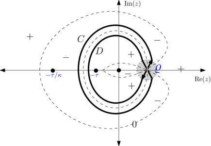
Figure 7. Zero contours for $\operatorname{Re}(G(z))-\operatorname{Re}(G(\varrho))$ are depicted by dashed lines (with the number 0 marked along them). Between these dashed lines lie areas of positive and negative real part, indicated by the occurrence of plus and minus signs. The contours $C$ and $D$ are depicted by solid lines. The region of the contours around the $\varrho$ are blown up on Figure 8 the right and coincide locally with the limiting contours $\tilde{C}$ and $\tilde{D}$.

We can now conclude about the features of the level lines (solutions) $\operatorname{Re}(G(z))=\operatorname{Re}(G(\varrho))$. Namely, the level lines form $3$ closed loops as shown in Figure 7: all the loops pass through $\varrho$, their second points of intersection with real axis lie on the intervals $(-\infty,-\tau/\kappa)$, $(-\tau/\kappa,-\tau)$ and $(-\tau,0)$, respectively. The sign of $\operatorname{Re}(G(z))-\operatorname{Re}(G(\varrho)$ alternates over the domains bounded by level lines, as shown in Figure 7.

Finally, we claim that all the loops are “star–shaped”, which means for each angle $\phi$ each loop has precisely one point $z$ satisfying $Arg(z)=\phi$. To prove that, we fix $z_{0}=x_{0}+\mathbf{i}y_{0}$ with $Arg(z_{0})=\phi$ (we can assume that $0<\phi<\pi$ and the case of real $z$ was studied before) and consider the function of real variable $q$ given by

$$\operatorname{Re}\bigl{(}G(z_{0}q)\bigr{)}=\ln\big{|}1+z_{0}q\kappa\tau^{-1}\big{|}-\nu\ln\big{|}1+z_{0}q\tau^{-1}\big{|}+m_{\nu}\ln|z_{0}q|.$$

Note that we allow $q$ to be negative here. We have

$$\frac{\partial}{\partial q}\operatorname{Re}\bigl{(}G(z_{0}q)\bigr{)}=\operatorname{Re}\left(\frac{z_{0}\kappa\tau^{-1}}{1+z_{0}q\kappa\tau^{-1}}-\frac{\nu z_{0}\tau^{-1}}{1+z_{0}q\tau^{-1}}+\frac{m_{\nu}}{q}\right)$$

The last formula implies that the roots of $\frac{\partial}{\partial q}\operatorname{Re}(G(z_{0}q)=0$ are the roots of a degree $4$ polynomial (in $q$) and, thus, there are at most $4$ of them. Taking into the account the singularity at $0$ we conclude that for each $W\in\mathbb{R}$ the equation $\operatorname{Re}(G(z_{0}q))=W$ has at most $6$ solutions: Indeed, there are $m$ positive solutions and $n$ negative solutions, between each solution a root of the derivative should exist, thus, $(m-1)+(n-1)\leq 4$.

Now if all the loops of $\operatorname{Re}(G(z))=\operatorname{Re}(G(\varrho))$ are star-shaped, then this already gives precisely $6$ solutions; if one of the loops were not star–shaped, then we would have had more solutions, which is impossible.

After having established the validity of Figure 7 we proceed to the contour deformations. We deform the $w$–contour and $v$–contour to curves $C$ and $D$, shown in Figure 7, respectively. The $w$–contour $C$ goes through the critical point $\varrho$ and departs it at angles $\pm\pi/3$ (oriented with increasing imaginary part). Likewise, the $v$ contour $D$ goes through $\varrho-\varrho\sigma_{\nu}^{-1}L^{-1/3}$ and departs at angles $\pm 2\pi/3$ (oriented with decreasing imaginary part – as is a consequence of the change of variables). The reason for the shift in the location of the $v$ contour is to avoid the pole from the denominator $v-w^{\prime}$. Outside a small neighborhood of $\varrho$ both contours closely follow one of the loops of $\operatorname{Re}(G(z))=\operatorname{Re}(G(\varrho))$ — the one which is between them and then crosses the negative real axis between $-\tau/\kappa$ and $-\tau$. The $C$ contour stays outside this loop, i.e. $\operatorname{Re}(G(w))-\operatorname{Re}(G(\varrho))<0$ along it (for $z\neq\varrho$), while the $D$ contour is inside the loop and $\operatorname{Re}(G(v))-\operatorname{Re}(G(\varrho))>0$ along it (outside a small neighborhood of $\varrho$).

As a consequence, on the new contours $C$ and $D$, for any $\varepsilon>0$ there exists $\delta>0$ such that as long as either $w$ or $v$ is outside $\varepsilon$–neighborhood of $\varrho$, we have $\operatorname{Re}(G(w))-\operatorname{Re}(G(v))<\delta$. Therefore, the integrand in (67) would decay exponentially fast as $L\to\infty$. It follows (see Section 5.2) that asymptotically only $w$, $v$ in a small neighborhood of $\varrho$ influence the desired Fredholm determinant.

Figure 8. The contours $\tilde{C}$ and $\tilde{D}$ in $\tilde{z}$ plane obtained from $C$ and $D$ in $z$ plane after the change of variables $z=\varrho+L^{-1/3}\varrho\sigma_{\nu}^{-1}\tilde{z}$. The variable $\tilde{w}$ is integrated over $\widetilde{C}$ and $\tilde{v}$ is integrated over $\widetilde{D}$.

In a small neighborhood of $\varrho$ we make a change of variables $w=\varrho+L^{-1/3}\varrho\sigma_{\nu}^{-1}\tilde{w}$, $v=\varrho+L^{-1/3}\varrho\sigma_{\nu}^{-1}\tilde{v}$. The contours arising after this change of variables are shown in Figure 8. Note that we have integration both in $v$ (in (67)) and in $w$ (in the definition of Fredholm determinant), this means that we should also absorb in the kernel $K$ the factor $L^{-2/3}\varrho^{2}\sigma_{\nu}^{-2}$ arising from the Jacobian of the change of coordinates. As a result, using the Taylor expansion (68) and the expansion $\ln(\varrho+z)=\ln(\varrho)+z/\varrho+o(z)$, the kernel in (67) transforms into

$$\tilde{K}^{b_{1},b_{2}}_{\zeta(L)}(\tilde{w},\tilde{w}^{\prime})=\frac{L^{-1/3}\varrho\sigma_{\nu}^{-1}}{\ln(\tau)2\mathbf{i}}\sum_{k=-\infty}^{\infty}\int_{\widetilde{D}}\frac{\exp\left[\frac{\tilde{w}^{3}}{3}-\frac{\tilde{v}^{3}}{3}+h(\tilde{v}-\tilde{w})+o(1)\right]\cdot d\tilde{v}}{(\tilde{v}-\tilde{w}^{\prime})\sin\left(\frac{\pi}{\ln(\tau)}(L^{-1/3}\sigma_{\nu}^{-1}(\tilde{v}-\tilde{w})+2\pi\mathbf{i}k)\right)(\varrho+o(1))}.$$ (69)

When $k\neq 0$,

$$\lim_{L\to\infty}\sin\left(\frac{\pi}{\ln(\tau)}(L^{-1/3}\sigma_{\nu}^{-1}(\tilde{v}-\tilde{w})+2\pi\mathbf{i}k)\right)=\sin\left(\frac{\pi}{\ln(\tau)}2\pi\mathbf{i}k\right)\neq 0,$$

and the corresponding term in the summation of $k$ vanishes due to the $L^{-1/3}$ prefactor. On the other hand, when $k=0$, as $L\to\infty$

$$\sin\left(\frac{\pi}{\ln(\tau)}(L^{-1/3}\sigma_{\nu}^{-1}(\tilde{v}-\tilde{w}))\right)\approx\frac{\pi}{\ln(\tau)}L^{-1/3}\sigma_{\nu}^{-1}(\tilde{v}-\tilde{w})$$

Plugging this into (69), we conclude that

$$\lim_{L\to\infty}\tilde{K}^{b_{1},b_{2}}_{\zeta(L)}(\tilde{w},\tilde{w}^{\prime})=\frac{1}{2\pi\mathbf{i}}\int_{\widetilde{D}}\frac{\exp\left[\frac{\tilde{w}^{3}}{3}-\frac{\tilde{v}^{3}}{3}+h(\tilde{v}-\tilde{w})\right]\cdot d\tilde{v}}{(\tilde{v}-\tilde{w}^{\prime})(\tilde{v}-\tilde{w})}.$$ (70)

Denoting the right–side of (70) as $K^{Ai}$, we conclude that

$$\lim_{L\to\infty}\det\left(1+K^{b_{1},b_{2}}_{\zeta(L)}\right)_{C_{r}}=\det\left(1+K^{Ai}\right)_{\widetilde{C}}.$$ (71)

The last determinant is (upon a change of variables $\tilde{v}\to-\tilde{v}$, $\tilde{w}\to-\tilde{w}$, $\tilde{w}^{\prime}\to-\tilde{w}^{\prime}$) a standard expression for $F_{GUE}(h)$, cf. [TW2], [BCF, Lemma 8.6].

5.2. On the estimates

In the argument of Section 5.1 we were dealing with leading terms of the asymptotics without making the estimates for the remainders. All such estimates are fairly standard, let us only point where they are required and where analogous estimates can be found in the literature.

1. In order to justify formula (69) and the following pointwise limit in it, we need to estimate the integral outside a small neighborhood of the critical point $\varrho$. This is a usual estimate of steepest descent method of the analysis of integrals, cf. [Cop], [Er]. In the related context of directed polymers in random media a very similar justifications were done recently in [BCF, Section 5.2], [BCR, Section 2].

2. The formula (70) leads to the termwise limit for the Fredholm determinant of Proposition 5.3. To justify the $L\to\infty$ limit for the sums, i.e. equality (71) we need also certain uniform estimates for the remainder of the series (large $n$ terms of Definition 4.13). Using Hadamard’s inequality this readily follows from our limit analysis of the kernel $K^{b_{1},b_{2}}_{\zeta(L)}$ and we again refer to [BCF, Section 5.2], [BCR, Section 2] and references therein for additional details.

6. Proofs of Theorem 1.1 and Theorem 1.2

Due to the identification between the the configurations of the six–vertex model and interacting particle system $\mathbf{X}^{b_{1},b_{2}}(t)$ explained in Section 2.2, $H(x,y;\omega)$ of Theorem 1.2 is the same as $N_{x}(t)$ with $t=y$ of Theorem 5.1. Thus, these theorems are equivalent, and passing from one to another is a matter of changing the notations.

Further, Theorem 1.2 readily implies Theorem 1.1 for $x,y$ satisfying $\frac{1-b_{1}}{1-b_{2}}<\frac{x}{y}<\frac{1-b_{2}}{1-b_{1}}$.

Let us study the remaining $x,y$. We start from $x\leq\frac{1-b_{1}}{1-b_{2}}y$. Choose any $\varepsilon>0$ and write

$$\limsup_{L\to\infty}\frac{H(Lx,Ly;\omega)}{L}\leq\limsup_{L\to\infty}\frac{H(L(\frac{1-b_{1}}{1-b_{2}}y+\varepsilon),Ly;\omega)}{L}=\mathcal{H}\left(\frac{1-b_{1}}{1-b_{2}}y+\varepsilon,y\right).$$

The definition of $\mathcal{H}$ implies that for any $y$,

$$\lim_{\varepsilon\to 0}\mathcal{H}\left(\frac{1-b_{1}}{1-b_{2}}y+\varepsilon,y\right)=0.$$

Since $H(Lx,Ly;\omega)\geq 0$ we conclude that for $x,y$ satisfying $\frac{x}{y}\leq\frac{1-b_{1}}{1-b_{2}}$ we have

$$\lim_{L\to\infty}\frac{H(Lx,Ly;\omega)}{L}=0.$$

It remains to consider the case $x\geq\frac{1-b_{2}}{1-b_{1}}y$. For this note that for any $x$, $y>0$ we have (almost surely)

$$H(x,y;\omega)\geq L(x-y)-2.$$

To prove this inequality observe that $H(x,0;\omega)=\lfloor x\rfloor$ and when we increase $y$ by $1$ the height function decreases at most by $1$. Therefore,

$$\liminf_{L\to\infty}\frac{H(Lx,Ly;\omega)}{L}\geq x-y.$$ (72)

On the other hand, for $x\geq\frac{1-b_{2}}{1-b_{1}}y$ and any $\varepsilon>0$ we have (again using the fact that $H$ does not change by more than one as we move by one unit along the grid)

$$H(Lx,Ly;\omega)\leq H\left(L\left(\frac{1-b_{2}}{1-b_{1}}y-\varepsilon\right),Ly;\omega\right)+L\left(x-\frac{1-b_{2}}{1-b_{1}}y\right)+1.$$ (73)

Using the definition of the limit $\mathcal{H}(x,y)$ we see that for any $y$

$$\lim_{\varepsilon\to 0}\mathcal{H}\left(\frac{1-b_{2}}{1-b_{1}}y-\varepsilon,y\right)=\frac{1-b_{2}}{1-b_{1}}y-y.$$ (74)

Therefore, sending $L\to\infty$ in (73) we conclude that (in probability)

$$\limsup_{L\to\infty}\frac{H(Lx,Ly;\omega)}{L}\leq\left(\frac{1-b_{2}}{1-b_{1}}y-y\right)+\left(x-\frac{1-b_{2}}{1-b_{1}}y\right)=x-y.$$ (75)

Combining (72) and (75) we conclude that for $x\geq\frac{1-b_{2}}{1-b_{1}}y$,

$$\lim_{L\to\infty}\frac{H(Lx,Ly;\omega)}{L}=x-y,$$

which finishes the proof of Theorem 1.1.

References

- [ACQ] G. Amir, I. Corwin, J. Quastel. Probability distribution of the free energy of the continuum directed random polymer in 1 + 1 dimensions. Communications on Pure and Applied Mathematics, 64 (2011), 466–537. arXiv:1003.0443.
- [ADW] G. Albertini, S. R. Dahmen, B. Wehefritz, Phase diagram of the non-Hermitian asymmetric XXZ spin chain, Journal of Physics A: Mathematical and General, 29 (1996) L369 L376.
- [AAR] G. Andrews, R. Askey, R. Roy. Special functions. Cambridge University Press, 2000.
- [Bax] R. J. Baxter, Exactly solved models in statistical mechanics, The Dover Edition, Dover, 2007.
- [BeGi] L. Bertini, G. Giacomin, Stochastic Burgers and KPZ equations from particle system, Communications in Mathematical Physics, 183 (1997), 571–607.
- [BFZ] R. E. Behrend, P. Di Francesco, P. Zinn–Justin, On the weighted enumeration of alternating sign matrices and descending plane partitions, Journal of Combinatorial Theory, Series A, 119, no. 2 (2012), 331–363. arXiv:1103.1176.
- [Bor] A. Borodin, CLT for spectra of submatrices of Wigner random matrices, Moscow Mathematical Journal, 14, no. 1 (2014), 29–38, arXiv:1010.0898.
- [BC] A. Borodin, I. Corwin, Macdonald processes, Probability Theory and Related Fields, 158 (2014) 225–400, arXiv:1111.4408
- [BCF] A. Borodin, I. Corwin, P. Ferrari, Free energy fluctuations for directed polymers in random media in 1+1 dimension, to appear in Communications on Pure and Applied Mathematics, arXiv:1204.1024
- [BCPS] A. Borodin, I. Corwin, L. Petrov, T. Sasamoto, Spectral theory for interacting particle systems solvable by coordinate Bethe ansatz, in preparation.
- [BCS] A. Borodin, I. Corwin and T. Sasamoto. From duality to determinants for -TASEP and ASEP, to appear in Annals of Probability, arXiv:1207.5035
- [BCR] A. Borodin, I. Corwin, D. Remenik, Log-Gamma polymer free energy fluctuations via a Fredholm determinant identity, Communications in Mathematical Physics, 324 (2013), 215–232, arXiv:1206.4573.
- [BF1] A. Borodin, P. Ferrari, Large time asymptotics of growth models on space-like paths I: PushASEP, Electron. J. Probab. 13 (2008), 1380–1418. arXiv:0707.2813.
- [BF2] A. Borodin, P. Ferrari, Anisotropic growth of random surfaces in 2 + 1 dimensions, Communications in Mathematical Physics, 325, no. 2 (2014), 603–684. arXiv:0804.3035.
- [BG] A. Borodin, V. Gorin, General beta Jacobi corners process and the Gaussian free field, to appear in Communications on Pure and Applied Mathematics. arXiv:1305.3627.
- [BG2] A. Borodin, V. Gorin. Lectures on integrable probability. arXiv:1212.3351.
- [BP] A. Borodin, L. Petrov, Integrable probability: from representation thery to Macdonald processes, Probability Surveys, 11 (2014), 1–58. arXiv:1310.8007.
- [Br] D. M. Bressoud, Proofs and confirmations: the story of the alternating sign matrix conjecture, Cambridge Univ. Press, Cambridge, 1999.
- [CKP] H. Cohn, R. Kenyon, J. Propp, A variational principle for domino tilings. Journal of American Mathematical Society, 14 (2001), no. 2, 297-346. arXiv:math/0008220.
- [Cop] E. T. Copson, Asymptotic expansions, Cambridge University Press, 1965.
- [Cor1] I. Corwin. The Kardar-Parisi-Zhang equation and universality class, Random Matrices: Theory and Applications, 1, no. 1 (2012). arXiv:1106.1596
- [Cor2] I. Corwin, Two ways to solve ASEP. Pan-American Summer Institute: Topics in Percolative and Disordered Systems, Springer, arXiv:1212.2267
- [Cor3] I. Corwin, Macdonald processes, quantum integrable systems and the Kardar-Parisi-Zhang universality class, Proceedings of ICM 2014 in Seoul. arXiv:1403.6877
- [CDR] P. Calabrese, P. Le Doussal, A. Rosso. Free-energy distribution of the directed polymer at high temperature, European Physical Letters, 90:20002 (2010). arXiv:1002.4560.
- [D] V. Dotsenko. Bethe ansatz derivation of the Tracy-Widom distribution for one dimensional directed polymers. European Physical Letters, 90:20003 (2010). arXiv:1003.4899.
- [EKLP] N. Elkies, G. Kuperberg, M. Larsen, J. Propp, Alternating-sign matrices and domino tilings. I,II, Journals of Algebraic Combinatorics, 1 (1992), no. 2, 111–132; no. 3, 219-234. arXiv:math/9201305.
- [Er] A. Erdelyi, Asymptotic Expansions, Dover Publications, 1956.
- [FS1] P. Ferrari, H. Spohn, Domino tilings and the six-vertex model at its free fermion point, Journal of Physics A: Mathematical and General, 39 (2006), 10297–10306, arXiv:cond-mat/0605406.
- [FS2] P. L. Ferrari and H. Spohn, Random growth models. In: The Oxford Handbook of Random Matrix Theory, G. Akemann, J. Baik, P. Di Francesco (editors), Oxford University Press, 2011, arXiv:1003.0881.
- [FV] P. Ferrari, B. Veto, Tracy-Widom asymptotics for -TASEP, arXiv:1310.2515.
- [GH] H.-O. Georgii, Y. Higuchi, Percolation and number of phases in the two-dimensional Ising model, Journal of Mathematical Physics 41, no. 3(2000), 1153–1169.
- [Gi] J. de Gier, Fully packed loop models on finite geometries, Polygons, polyominoes and polycubes, Lecture Notes in Physics, vol. 775, 2009, arXiv:0901.3963.
- [G1] V. Gorin, The -Gelfand-Tsetlin graph, Gibbs measures and -Toeplitz matrices, Advances in Mathematics, 229 (2012), no. 1, 201–266. arXiv:1011.1769.
- [G] V. Gorin, From alternating sign matrices to the Gaussian unitary ensemble, Communications in Mathematical Physics, 2014. arXiv:1306.6347.
- [GP] V. Gorin, G. Panova, Asymptotics of symmetric polynomials with applications to statistical mechanics and representation theory, to appear in Annals of Probability. arXiv:1301.0634.
- [GS] L.-H. Gwa, H. Spohn, Six-vertex model, roughened surfaces, and an asymmetric spin Hamiltonian, Physical Review Letters, 68, no. 6 (1992), 725–728.
- [HJ] R. A. Horn, C. R. Johnson, Matrix Analysis, Second Edition, Cambridge University Press, 2013.
- [JS] C. Jayaprakash, A. Sinha, Commuting transfer matrix solution of the asymmetric six–vertex model, Nuclear Physics B210 [FS6] (1982) 93-102
- [J1] K. Johansson, Shape fluctuations and random matrices, Communications in Mathematical Physics, 209 (2000), 437–476. arXiv:math/9903134.
- [J2] K. Johansson, Discrete polynuclear growth and determinantal processes, Communications in Mathematica Physics, 242 (2003), 277–329, arXiv:math/0206208.
- [J3] K. Johansson, The arctic circle boundary and the Airy Process, The Annals of Probability, 33, no. 1 (2005), 1–30
- [JN] K. Johansson, E. Nordenstam, Eigenvalues of GUE minors. Electronic Journal of Probability 11 (2006), paper 50, 1342-1371. arXiv:math/0606760
- [KPZ] M. Kardar, G. Parisi, and Y.-C. Zhang, Dynamic Scaling of Growing Interfaces, Physical Review Letters, 56 (1986), 889–892.
- [KO] R. Kenyon, A. Okounkov, Limit shapes and Burgers equation, Acta Mathematica, 199 (2007), no. 2, 263–302. arXiv:math-ph/0507007.
- [KOS] R. Kenyon, A. Okounkov, and S. Sheffield, Dimers and amoebae, Annals of Mathematics, 163 (2006), 1019–1056, arXiv:math-ph/0311005
- [Ken] R. Kenyon, Height fluctuations in the honeycomb dimer model, Communications in Mathematical Physics, 281, no. 3 (2008), 675–709, arXiv: math-ph/0405052
- [Ki] D. Kim, Asymmetric XXZ chain at the antiferromagnetic transition: spectra and partition functions, Journal of Physics A: Mathematical and General, 30 (1997) 3817–3836
- [Ku] G. Kuperberg, Another proof of the alternating-sign matrix conjecture, International Mathematics Research Notices, (1996), 139–150. arXiv:math.CO/9712207.
- [Lig1] T. Liggett, Interacting Particle Systems, Springer-Verlag, New York, 1985.
- [Lig2] T. Liggett, Stochastic interacting systems: contact, voter and exclusion Processes. Grundlehren der mathematischen Wissenschaften, volume 324, Springer, 1999.
- [L] E. H. Lieb, The residual entropy of square ice, Physical Review 162, 162-172 (1967)
- [M] I. G. Macdonald, Symmetric functions and Hall polynomials, Second Edition. The Clarendon Press, Oxford University Press, New York, 1995
- [N] I. M. Nolden, The asymmetric six-vertex model, Journal of Statistical Physics, 67, nos. 1/2 (1992).
- [PR] K. Palamarchuk, N. Reshetikhin, The 6-vertex model with fixed boundary conditions, Proceedings of Solvay Workshop “Bethe Ansatz : 75 Years Later”, arXiv:1010.5011
- [P] L. Petrov, Asymptotics of uniformly random lozenge tilings of polygons. Gaussian Free Field, to appear in Annals of Probability, arXiv:1206.5123.
- [PS2] M. Prahofer, H. Spohn, Universal distributions for growth processes in 1 + 1 dimensions and random matrices, Physical Review Letters, 84, no. 21 (2000), 4882–4885, arXiv:cond-mat/9912264.
- [PS2] M. Prahofer, H. Spohn, Scale invariance of the PNG droplet and the Airy process, Journal of Statistical Physics, 108 (2002), 1071–1106, arXiv:math/0105240
- [Resh] N. Reshetikhin, Lectures on the integrability of the 6-vertex model, arXiv:1010.5031
- [Rez] F. Rezakhanlou, Continuum limit for some growth models, Stochastic Processes and their Applications, 101 (2002), 1–41.
- [Ro] H. Rost, Nonequilibrium behaviour of a many particle process: density profile and local equilibria. Zeitschrift fur Wahrscheinlichkeitstheorie und Verwandte Gebiete, 58, no. 1 (1981), 41–53.
- [SS] T. Sasamoto, H. Spohn. One-dimensional KPZ equation: an exact solution and its universality. Physical Review Letters, 104, 230602 (2010). arXiv:1002.1883
- [Se] T. Seppalainen, Hydrodynamic scaling, convex duality and asymptotic shapes of growth models. Markov Processes and Related Fields, 4 (1998), 1–26.
- [Sh] S. Sheffield, Random surfaces, Asterisque 2005, no. 304, arXiv:math/0304049.
- [Spi] F. Spitzer, Interaction of Markov processes, Advances in Mathematics, 5, no. 2 (1970), 246–290.
- [Spo1] H. Spohn, Large scale dynamics of interacting particles, Springer, 1991
- [Spo2] H. Spohn, KPZ Scaling Theory and the semi-discrete directed polymer model, MSRI Proceedings, arXiv:1201.0645.
- [TW1] C. Tracy, H. Widom, Level-spacing distributions and the Airy kernel, Communications in Mathematical Physics, 159, no. 1 (1994), 151–174.
- [TW2] C. Tracy, H. Widom, Integral formulas for the asymmetric simple exclusion process, Communications in Mathematical Physics, 279, 815–844 (2008). Erratum: Communication in Mathematical Physics, 304, 875–878 (2011), arXiv:0704.2633
- [TW3] C. Tracy, H. Widom, Asymptotics in ASEP with step initial condition. Communications in Mathematical Physics, 290 (2009), 129–154, arXiv:0807.1713
- [TW4] C. Tracy, H. Widom, Formulas and asymptotics for the asymmetric simple exclusion process, Mathematical Physics, Analysis and Geometry 14 (2011), 211–235, arxiv:1101.2682
- [Z] P. Zinn-Justin, Six-Vertex, loop and tiling models: integrability and combinatorics, arXiv:0901.0665