Analytic Calculation of 1-Jettiness in DIS at $\mathcal{O}(\alpha_{s})$

Abstract

We present an analytic $\mathcal{O}(\alpha_{s})$ calculation of cross sections in deep inelastic scattering (DIS) dependent on an event shape, 1-jettiness, that probes final states with one jet plus initial state radiation. This is the first entirely analytic calculation for a DIS event shape cross section at this order. We present results for the differential and cumulative 1-jettiness cross sections, and express both in terms of structure functions dependent not only on the usual DIS variables $x,Q^{2}$ but also on the 1-jettiness $\tau$. Combined with previous results for log resummation, predictions are obtained over the entire range of the 1-jettiness distribution.

1 Introduction

In high energy colliders, jet production plays an important role in probing the strong interaction, hadron structure, dense media, and new particles beyond the Standard Model. Thus predicting jet production cross sections and jet structure is one of the important tasks of Quantum Chromodynamics (QCD). Jet algorithms Catani:1991hj ; Catani:1993hr ; Ellis:1993tq ; Dokshitzer:1997in ; Salam:2007xv ; Cacciari:2008gp allow exclusive study of jets and definitions of cross sections with a definite number of jets. However, they also introduce various parameters like jet radii or sizes and jet vetoes, which require more effort to predict accurately in analytic calculations in QCD. Event shapes Dasgupta:2003iq provide a simple, inclusive way to identify final states that are jet-like, and can often be predicted to very high accuracy in QCD. Thrust in $e^{+}e^{-}$ collisions Farhi:1977sg is a classic example of a two-jet event shape that has been extensively studied in both theory and experiment. Thrust cross sections in $e^{+}e^{-}$ have been predicted to very high accuracy, N³LL$+\mathcal{O}(\alpha_{s}^{3})$ in resummed and fixed-order perturbation theory GehrmannDeRidder:2007bj ; GehrmannDeRidder:2007hr ; Weinzierl:2008iv ; Weinzierl:2009ms ; Becher:2008cf ; Abbate:2010xh , along with rigorous treatments of nonperturbative power corrections Lee:2006nr ; Abbate:2010xh ; Mateu:2012nk , that have led to unprecedented 1%-level precision in determinations of the strong coupling constant $\alpha_{s}$ from $e^{+}e^{-}$ event shape data Becher:2008cf ; Chien:2010kc ; Abbate:2010xh .

Event shapes in DIS have also been studied but not as extensively as in $e^{+}e^{-}$, and the theoretical accuracy has yet to catch up to the same level. Two versions of DIS thrust have been defined and measured in H1 and ZEUS experiments at HERA Adloff:1997gq ; Adloff:1999gn ; Aktas:2005tz ; Breitweg:1997ug ; Chekanov:2002xk ; Chekanov:2006hv and they have been calculated up to next-leading-logarithmic accuracy (NLL) at resummed order and numerically to $\mathcal{O}(\alpha_{s}^{2})$ at fixed order Antonelli:1999kx ; Dasgupta:2002dc . The measured DIS thrusts involve non-global logarithms (NGLs), which present a theoretical obstacle to higher order accuracy Dasgupta:2001sh ; Dasgupta:2002dc .

Versions of thrust such as $e^{+}e^{-}$ thrust and the DIS thrust $\tau_{Q}$ defined in Antonelli:1999kx do not suffer from NGLs. A class of event shapes called $N$-jettiness $\tau_{N}$ Stewart:2010tn is a generalization of these versions of thrust and are applicable in different collider environments, including $e^{+}e^{-}$, lepton-hadron, and hadron-hadron collisions. $\tau_{N}$ measures the degree of collimation of final-state hadrons along $N$ light-like directions in addition to any initial-state radiation (ISR) along the incoming beam directions. In a number of recent papers Kang:2013nha ; Kang:2012zr ; Kang:2013wca , factorization theorems for various versions of 1-jettiness $\tau$ in DIS have been derived by using soft collinear effective theory (SCET) Bauer:2000ew ; Bauer:2000yr ; Bauer:2001ct ; Bauer:2001yt ; Bauer:2002nz . To date, this has enabled log resummation up to NNLL accuracy Kang:2013nha ; Kang:2012zr ; Kang:2013wca , which is one order higher in resummed accuracy than earlier results Antonelli:1999kx ; Dasgupta:2002dc .

The SCET results Kang:2013nha ; Kang:2012zr ; Kang:2013wca correctly capture and resum all logarithmic terms (singular), while non-logarithmic terms (nonsingular) can be obtained from fixed-order computations in full QCD. The full cross section is the sum of singular and nonsingular parts and can be written as

$$\sigma^{\text{full}}(\tau)=\sigma^{\text{sing}}(\tau)+\sigma^{\text{ns}}(\tau)\,.$$ (1)

The singular part is factorized in terms of hard, jet, beam, and soft functions each of which depends on the relevant energy scale for each mode Kang:2013nha ; Kang:2012zr ; Kang:2013wca . This separation of scales and renormalization group (RG) evolution between them allows for resummation of the large logarithms in the fixed-order expansion of the cross section. When the RG evolution is turned off in the singular part, the full cross section reduces to the ordinary fixed-order result. The nonsingular part is obtained by subtracting the fixed-order singular part from the fixed-order cross section.

For an accurate prediction over the entire range of an event shape distribution, both fixed-order and resummed calculations should be consistently improved. While NNLL resummation of the singular part in Eq. (1) has been performed for three different versions of DIS 1-jettiness in Kang:2013nha and another version in Kang:2012zr ; Kang:2013wca , no analytic computations of the non-singular part at $\mathcal{O}(\alpha_{s})$ or above have yet been performed. In Kang:2013lga an $\mathcal{O}(\alpha_{s})$ result has been numerically obtained for a version of 1-jettiness that requires a jet algorithm to determine the jet momentum. Such a numerical approach is appropriate for such cases and allows for the flexibility of using different jet algorithms.

In this paper, we carry out the first analytic $\mathcal{O}(\alpha_{s})$ calculation for a DIS event shape. We choose the version of 1-jettiness called $\tau_{1}^{b}$ in Kang:2013nha , which groups final-state particles into back-to-back hemispheres in the Breit frame and is the same as the DIS thrust called $\tau_{Q}$ in Ref. Antonelli:1999kx . It can be written as

$$\tau=\frac{2}{Q^{2}}\sum_{i\in X}\min\{q_{B}^{b}\!\cdot\!p_{i},q_{J}^{b}\!\cdot\!p_{i}\}\stackrel{{\scriptstyle\text{Breit}}}{{=}}1-\frac{2}{Q}\sum_{i\in\mathcal{H}_{J}}p_{i\,z}\,,$$ (2)

where $p_{i}$ is the momentum of the $i$th particle in the final state, and $Q^{2}\equiv-q^{2}$ is determined by the momentum transfer $q$ in the event. The reference vectors are defined by $q_{B}^{b}=xP$ and $q_{J}^{b}=q+xP$, where $P$ is the proton momentum. In the Breit frame these vectors point exactly back-to-back. The second definition in Eq. (2) is valid in the Breit frame, and requires measuring the $z$ components $p_{i\,z}$ of momenta of particles only in the jet hemisphere (current hemisphere) $\mathcal{H}_{J}$. The definition in Eq. (2) differs from the measured version $\tau^{\text{H1}}=1-T_{\gamma}^{\text{ZEUS}}$ Aktas:2005tz ; Chekanov:2006hv in normalization (replacing $2/Q$ by $1/E_{\rm hemi}$ where $E_{\rm hemi}$ is the hemisphere energy).

We present our results in terms of fixed-order singular and nonsingular parts of the cross section as in Eq. (1). They can be put in a simple form which can easily be implemented in other analyses. The main new results of this paper are the nonsingular 1-jettiness structure functions given by Eq. (43).

We also show numerical results with perturbative uncertainties by varying scales at the HERA energy. Our results could be compared to existing HERA data Adloff:1997gq ; Adloff:1999gn ; Aktas:2005tz ; Breitweg:1997ug ; Chekanov:2002xk ; Chekanov:2006hv or to future EIC data Accardi:2012hwp . In Kang:2013nha , by comparing our resummed singular cross section to the known fixed-order total cross section, we estimated that the nonsingular corrections would amount to several percent of the total cross section, and this expectation is borne out by our computations here.

The paper is organized as follows: In Sec. 2 we briefly review the relevant kinematic variables in DIS and our definition of 1-jettiness, and express the cross section in terms of structure functions. In Sec. 3, we outline the basic steps of the $\mathcal{O}(\alpha_{s})$ computation including the phase space for 1-jettiness and perturbative matching of the hadronic tensor onto parton distribution functions (PDFs). Sec. 4 contains our main results, analytic $\mathcal{O}(\alpha_{s})$ expressions for 1-jettiness structure functions. Details of the fixed-order calculation are given in App. A, App. B and App. C. In Sec. 5 numerical results are given for structure functions at $\mathcal{O}(\alpha_{s})$ fixed-order accuracy and cross sections at NLL${}^{\prime}+\mathcal{O}(\alpha_{s})$ resummed accuracy. Basic details entering the resummation of the singular terms are reviewed in App. D and App. E for convenience. Finally, we will conclude in Sec. 6.

2 1-Jettiness in DIS

In this section we review DIS kinematic variables that will be used throughout the paper and the definition of the 1-jettiness $\tau$ cross section in DIS, whose computation will be the main prediction of our paper.

2.1 Kinematic Variables

In DIS, an incoming electron with 4-momentum $k$ scatters off a proton with momentum $P$ by exchanging a virtual photon with a large momentum transfer $q=k-k^{\prime}$, where $k^{\prime}$ is the momentum of the outgoing electron. Because the photon has spacelike momentum it has a negative virtuality, and one can define the positive definite quantity

$$Q^{2}\equiv-q^{2}\,.$$ (3)

$Q$ sets the momentum scale of the scattering. We will be interested in hard scattering, where $Q\gg\Lambda_{\text{QCD}}$. A dimensionless quantity $x$ called the Björken scaling variable is defined by

$$x\equiv-\frac{q^{2}}{2P\!\cdot\!q}=\frac{Q^{2}}{2P\!\cdot\!q},$$ (4)

which ranges between $0\leq x\leq 1$. Another dimensionless quantity $y$ is defined by $y\equiv\frac{2P\cdot q}{2P\cdot k}$, which ranges between $0\leq y\leq 1$. This variable $y$ represents the energy loss of the electron in the proton rest frame. The three variables $x$, $y$, and $Q^{2}$ are related to one another via $Q^{2}=xys$, where $s=(P+k)^{2}$ is the total invariant mass of the incoming particles. The total momentum of the final state $X$ is $p_{X}=q+P$ and the invariant mass is given by $p_{X}^{2}=\frac{1-x}{x}Q^{2}$. For large $x$ very near 1, the final state consists of a single tightly collimated jet of hadrons. This region has been analyzed in SCET in, e.g., Manohar:2003vb ; Chay:2005rz ; Becher:2006mr ; Chen:2006vd ; Fleming:2012kb . We will instead be interested in different region where two or more energetic jets can occur. This occurs in the “classic” region where $x$ has a generic size $x\sim 1-x\sim 1$ such that $p_{X}^{2}\sim Q^{2}$.

Although the cross section we compute is frame independent, there is a convenient frame in which to perform the intermediate steps of the calculation. This is the Breit frame, where the virtual photon with momentum $q^{\mu}$ is purely spacelike, and collides with the proton with momentum $P^{\mu}$ along the $z$ direction. In this frame the virtual photon and the proton have momenta

$$q^{\mu}=Q\frac{n_{z}^{\mu}-\bar{n}_{z}^{\mu}}{2}\,,\quad P^{\mu}=\frac{Q}{x}\frac{\bar{n}_{z}^{\mu}}{2}\,,$$ (5)

where $n_{z}=(1,0,0,1)$ and $\bar{n}_{z}=(1,0,0,-1)$.

2.2 $1$-Jettiness

To probe the number of jets in the final state produced at a given value of $x$ and $Q$, an additional measurement needs to be made. A simple event shape that accomplishes this is the $N$-jettiness Stewart:2010tn , a generalization of the thrust Farhi:1977sg . It is defined by the sum of projections of final-state particle momenta onto whichever axis is closest among $N$ jet and $N_{b}$ beam axes, where $N_{b}=0$ for $e^{+}e^{-}$ collisions, $1$ for $ep$ DIS, and 2 for $pp$ collisions. The $N$-jettiness $\tau_{N}$ is designed so that it becomes close to zero for an event with $N$ well-collimated jets in the final state away from any hadronic beam axes. For example, 1-jettiness in DIS is defined by one jet and one beam axis:

$$\tau_{1}\equiv\frac{2}{Q^{2}}\sum_{i\in X}\min\{q_{B}\!\cdot\!p_{i},q_{J}\!\cdot\!p_{i}\}\,,$$ (6)

where $q_{B},q_{J}$ are lightlike four-vectors along the beam and jet directions. It is natural to choose $q_{B}$ along the proton direction. One can consider several options for choosing $q_{J}$. In Kang:2013nha , we defined three versions of 1-jettiness $\tau_{1}^{a}$, $\tau_{1}^{b}$, and $\tau_{1}^{c}$ distinguished by different choices for $q_{J}$: (a) $q_{J}^{a}$ aligned along the jet axis determined by a jet algorithm, (b) $q_{J}^{b}$ along the $z$ axis in the Breit frame, and (3) $q_{J}^{c}$ along the $z$ axis in the center-of-momentum (CM) frame.

In this paper we consider $\tau_{1}^{b}$ for which $q_{B}^{b}$ and $q_{J}^{b}$ are given by

$${q_{B}^{b}}^{\mu}=xP^{\mu}\,,\quad{q_{J}^{b}}^{\mu}=q^{\mu}+xP^{\mu}\,.$$ (7)

As shorthand, we drop both superscript and subscript in $\tau_{1}^{b}$ throughout the remainder of the paper.

$$\tau\equiv\tau_{1}^{b}.$$ (8)

In the Breit frame, the vectors $q_{B,J}^{b}$ point exactly back-to-back with equal magnitude:

$$q_{B}^{b}\overset{\text{Breit}}{=}Q\frac{{\bar{n}}_{z}}{2}\,,\qquad q_{J}^{b}\overset{\text{Breit}}{=}Q\frac{n_{z}}{2}\,,$$ (9)

and divide particles in the final state into two equal hemispheres. One is the “beam” or “remnant” hemisphere $\mathcal{H}_{B}$ in the $-z$ direction and the other is the “jet” or “current” hemisphere $\mathcal{H}_{J}$ in the $+z$ direction.

The 1-jettiness $\tau$ in Eq. (8) has an experimental advantage in that it can be determined by measuring only one of the hemispheres, namely $\mathcal{H}_{J}$. This avoids having to measure the whole final state including the beam remnants, a technical difficulty in experiments such as H1 and ZEUS at HERA. By using $q$ and $P$ in the Breit frame in Eq. (5), the 1-jettiness can be written in the form

$$\tau\stackrel{{\scriptstyle\text{Breit}}}{{=}}\frac{1}{Q}\sum_{i\in X}\min\{\bar{n}_{z}\!\cdot\!p_{i},n_{z}\!\cdot\!p_{i}\}=1-\frac{2}{Q}\sum_{i\in\mathcal{H}_{J}}p_{i\,z}\,.$$ (10)

We used momentum conservation $p_{B}=p_{X}-p_{J}$, where $p_{B}=\sum_{i\in\mathcal{H}_{B}}p_{i}$ and $p_{J}=\sum_{i\in\mathcal{H}_{J}}p_{i}$. The definition Eq. (10) directly corresponds to the thrust $\tau_{Q}$ in DIS defined in Antonelli:1999kx . We can obtain the physical upper limit on $\tau$ using the kinematic constraints that the jet momentum $p_{J\,z}\geq 0$ has to be positive, and that the beam momentum’s $z$ component is negative, so that $p_{J\,z}=p_{X\,z}-p_{B\,z}\geq p_{X\,z}=Q\,(2x-1)/(2x)$. These conditions imply the upper limits on $\tau$:

$$\tau^{\text{max}}=\begin{cases}1&x\leq 1/2\,,\\ \frac{1-x}{x}&x\geq 1/2\,.\end{cases}$$ (11)

2.3 1-Jettiness Cross Section

The 1-jettiness cross section can be expressed in terms of leptonic and hadronic tensors:

$$\frac{d\sigma}{dx\,dQ^{2}\,d\tau}=L_{\mu\nu}(x,Q^{2})W^{\mu\nu}(x,Q^{2},\tau)\,,$$ (12)

where the lepton tensor for a photon exchange is given by

$$L_{\mu\nu}(x,Q^{2})=-\frac{\alpha^{2}}{2x^{2}s^{2}}\bigg{[}g_{\mu\nu}-2\frac{k^{\mu}k^{\prime\nu}+k^{\prime\mu}k^{\nu}}{Q^{2}}\bigg{]}\,,$$ (13)

where $k$ and $k^{\prime}$ are incoming and outgoing electron momenta and $\alpha\equiv\alpha_{\text{em}}$. The hadronic tensor is the current-current correlator in the proton state,

$$W^{\mu\nu}(x,Q^{2},\tau)=\int\,d^{4}x\,e^{iq\cdot x}\!\left\langle P\right\rvert\!J^{\mu{\dagger}}(x)\delta(\tau-\hat{\tau})J^{\nu}(0)\!\left\lvert P\right\rangle,$$ (14)

where $\hat{\tau}$ is a 1-jettiness operator that measures 1-jettiness when it acts on the final states, which we defined in Kang:2013nha , based on the construction of event shape measurement operators from the energy-momentum tensor in Sveshnikov:1995vi ; Cherzor:1997ak ; Belitsky:2001ij ; Bauer:2008dt . In this paper, we consider only the vector current $J^{\mu}=\sum_{f}Q_{f}\bar{q}_{f}\gamma^{\mu}q_{f}$. Previously we worked with both vector and axial-vector currents, see Kang:2013nha for the appropriate generalizations. Because the hadronic tensor depends only on the two momenta $P$ and $q$, it can be decomposed into products of tensors constructed with $g_{\mu\nu}$, $P^{\mu}$, $q^{\mu}$ and structure functions depending on $x$, $Q$, and $\tau$. In our conventions,

$$W^{\mu\nu}(x,Q^{2},\tau)=4\pi\biggl{[}T_{1}^{\mu\nu}\mathcal{F}_{1}(x,Q^{2},\tau)+T_{2}^{\mu\nu}\frac{\mathcal{F}_{2}(x,Q^{2},\tau)}{P\cdot q}\biggr{]}\,,$$ (15)

where the two tensor structures that appear are:

$$T_{1}^{\mu\nu}=-g^{\mu\nu}+\frac{q^{\mu}q^{\nu}}{q^{2}}\,,\quad T_{2}^{\mu\nu}=\Bigl{(}P^{\mu}-q^{\mu}\frac{P\cdot q}{q^{2}}\Bigr{)}\Bigl{(}P^{\nu}-q^{\nu}\frac{P\cdot q}{q^{2}}\Bigr{)}\,,$$ (16)

which arise from parity conservation and the Ward identity $q_{\mu}W^{\mu\nu}=W^{\mu\nu}q_{\nu}=0$. If we considered parity-violating scattering, e.g. with neutrinos, a third tensor $T_{3}^{\mu\nu}=-i\epsilon^{\mu\nu\alpha\beta}q_{\alpha}P_{\beta}$ would also appear.

In terms of the structure functions appearing in Eq. (15), the cross section Eq. (12) can be expressed

$$\frac{d\sigma}{dxdQ^{2}d\tau} =\frac{4\pi\alpha^{2}}{Q^{4}}\left[(1+(1-y)^{2})\mathcal{F}_{1}+\frac{1-y}{x}\mathcal{F}_{L}\right]\,,$$ (17)

where $\mathcal{F}_{L}\equiv\mathcal{F}_{2}-2x\mathcal{F}_{1}$. We use calligraphic font for the structure functions in the differential $\tau$ cross section. We will use Roman font $F_{1,L}$ for the structure functions in the integrated cross section, see Eqs. (39) and (40).

The structure functions $\mathcal{F}_{i}$ can be obtained by contracting the hadronic tensor with the metric tensor or the proton momentum $P^{\mu}$:

$$\mathcal{F}_{1}(x,Q^{2},\tau) =\frac{1}{8\pi(1-\epsilon)}\bigg{(}-g_{\mu\nu}W^{\mu\nu}+\frac{4x^{2}}{Q^{2}}P_{\mu}P_{\nu}W^{\mu\nu}\bigg{)}\,,$$

$$\mathcal{F}_{L}(x,Q^{2},\tau) =\frac{2x^{3}}{\pi Q^{2}}P_{\mu}P_{\nu}W^{\mu\nu}\,.$$ (18)

We choose to always work with expressions in $D=4-2\epsilon$ dimensions for the vector indices $\mu$ and $\nu$, so the factor of $1/(1-\epsilon)$ in $\mathcal{F}_{1}$ comes from taking the contraction $g_{\mu\nu}T_{1}^{\mu\nu}$. The contraction $P_{\mu}P_{\nu}W^{\mu\nu}$ turns out to be finite as $\epsilon\to 0$. The standard structure functions depend just on $x$ and $Q^{2}$, while those in Eq. (2.3) are additionally differential in $\tau$. The structure functions can be written in terms of singular and nonsingular parts as we did for the cross section in Eq. (1). We will present singular and nonsingular parts of the structure functions in Sec. 4, from which one easily obtains the corresponding parts of the cross section via Eq. (17).

3 Setup of the Computation

In this section we outline the basic steps in the $\mathcal{O}(\alpha_{s})$ computation of the 1-jettiness cross section in DIS. First, we describe the standard perturbative matching procedure for the hadronic tensor onto PDFs, which allows us to compute the matching coefficients using partonic external states. Then we set up the phase space integrals in the Breit frame in which the intermediate steps of the computation are simpler. The final results are frame independent. The reader who wishes to skip these details may turn directly to the final results in Sec. 4 and Sec. 5.

3.1 Perturbative Matching

Here, we describe the matching procedure to determine the short-distance coefficients that match the hadronic tensor $W_{\mu\nu}(x,Q^{2},\tau)$ onto PDFs. By using the operator product expansion (OPE) the hadronic tensor can be written in the factorized form

$$W^{h}_{\mu\nu}(x,Q^{2},\tau)=\sum_{i\in\{q,\bar{q},g\}}\int_{x}^{1}\frac{d\xi}{\xi}f_{i/h}(\xi,\mu)\,w^{i}_{\mu\nu}\Bigl{(}\frac{x}{\xi},Q^{2},\tau,\mu\Bigr{)}\,\,\biggl{[}1+\mathcal{O}\Bigl{(}\frac{\Lambda_{\text{QCD}}}{Q\tau}\Bigr{)}\biggr{]}\,,$$ (19)

where $f_{i/h}$ is the PDF for a parton $i\in\{q,\bar{q},g\}$ in a hadron $h$, and $w_{\mu\nu}^{i}$ is the short-distance coefficient that we will determine by perturbative matching. The sum over $q,\bar{q}$ goes over all light flavors $f\in\{u,d,s,c,b\}$ at the collision energies we consider. On the left-hand side of Eq. (19), the superscript $h$ specifies the hadron in the initial state. The coefficients $w_{\mu\nu}^{i}$ however can be computed in perturbation theory using any appropriate initial state including partonic ones. This is what we shall describe in this subsection.

The factorization theorem for an initial parton $j$ is given by

$$W_{\mu\nu}^{j} =\sum_{i\in\{q,\bar{q},g\}}f_{i/j}\otimes w_{\mu\nu}^{i}\,,$$ (20)

where the arguments are implicit for simplicity and the convolution integral over $\xi$ in Eq. (20) is replaced by the symbol $\otimes$. By comparing Eq. (20) to Eq. (19), all implicit notations can easily be recovered. We determine the coefficients $w^{i}$ by computing the $W_{\mu\nu}^{j}$, which are defined by Eq. (14) but with a quark or antiquark $j=q,\bar{q}$ or gluon $j=g$ in the initial state, and subtracting out the partonic PDFs, which are IR divergent and require a regulator. We perform this computation using dimensional regularization and defining PDFs in the $\overline{\text{MS}}$ scheme.

Working to $\mathcal{O}(\alpha_{s})$, and denoting the order $\alpha_{s}^{n}$ piece of each function by a superscript ⁽ⁿ⁾, Eq. (20) becomes

$$\begin{split}W_{\mu\nu}^{j\,(0)}&=\sum_{i\in\{q,\bar{q},g\}}f_{i/j}^{(0)}\otimes w_{\mu\nu}^{i\,(0)}\,,\\ W_{\mu\nu}^{j\,(1)}&=\sum_{i\in\{q,\bar{q},g\}}\Bigl{[}f_{i/j}^{(1)}\otimes w_{\mu\nu}^{i\,(0)}+f_{i/j}^{(0)}\otimes w_{\mu\nu}^{i\,(1)}\Bigr{]}\,.\end{split}$$ (21)

Using $\overline{\text{MS}}$ and using $\epsilon$ to regulate IR divergences, the partonic PDFs to $\mathcal{O}(\alpha_{s})$ are given by (see, e.g., Stewart:2010qs for related discussion)

$$\begin{split}f_{i/j}^{(0)}=\delta_{ij}\delta(1-z)\,,\qquad f_{i/j}^{(1)}=-\frac{1}{\epsilon}\frac{\alpha_{s}}{2\pi}C_{ij}P_{ij}(z)\,,\end{split}$$ (22)

where the color factors and splitting functions are given by

$$C_{qq^{\prime}}=C_{\bar{q}\bar{q}^{\prime}}=C_{F}\,,\quad P_{qq^{\prime}}(z)=P_{\bar{q}\bar{q}^{\prime}}(z)=\delta_{qq^{\prime}}P_{qq}(z)\,,$$ (23)

$$C_{qg}=C_{\bar{q}g}=T_{F}\,,\quad\ \ P_{\bar{q}g}(z)=P_{qg}(z)\,,\quad$$ (24)

with $P_{qq}(z)$ and $P_{qg}(z)$ given in Eq. (45) below. There are no contributions containing the splitting functions $P_{gq},P_{g\bar{q}},P_{gg}$ since the tensor $W_{\mu\nu}^{j}$ in Eq. (14) we compute contains only the quark current.

For the 1-jettiness structure functions Eq. (2.3), we only need the projections $-g_{\mu\nu}W^{\mu\nu}$ and $P_{\mu}P_{\nu}W^{\mu\nu}$ of the hadronic tensor in Eq. (3.1); hence, we obtain the projected coefficients $-g^{\mu\nu}w^{i}_{\mu\nu}$ and $P^{\mu}P^{\nu}w^{i}_{\mu\nu}$. We compute the contracted tensors $-g^{\mu\nu}W_{\mu\nu}^{i}$ explicitly in App. B. Including the factor of $(1-\epsilon)$ coming from the tensor contractions in $D$ dimensions, we obtain:

$$\frac{-g^{\mu\nu}W_{\mu\nu}^{q}(x,Q^{2},\tau)}{1-\epsilon} =4\pi Q_{f}^{2}\delta(1-x)\delta(\tau)+2\alpha_{s}C_{F}Q_{f}^{2}\Bigl{[}-\frac{1}{\epsilon}P_{qq}(x)\delta(\tau)+w_{G}^{q}(x,Q^{2},\tau)\Bigr{]}\,,$$ (25)

$$\frac{-g^{\mu\nu}W_{\mu\nu}^{g}(x,Q^{2},\tau)}{1-\epsilon} =4\alpha_{s}T_{F}\sum_{f}Q_{f}^{2}\Bigl{[}-\frac{1}{\epsilon}P_{qg}(x)\delta(\tau)+w_{G}^{g}(x,Q^{2},\tau)\Bigr{]}\,,$$ (26)

where $w_{G}^{q,g}$ are finite as $\epsilon\to 0$. For the quark tensor we consider one flavor $f$ at a time, since it will get convolved with a different PDF for each quark flavor, while for the gluon tensor we include the sum over all flavors. The contractions $P^{\mu}P^{\nu}W_{\mu\nu}^{i}$ begin at $\mathcal{O}(\alpha_{s})$, and take the form

$$P^{\mu}P^{\nu}W_{\mu\nu}^{i}(x,Q^{2},\tau)=\begin{cases}\alpha_{s}C_{F}Q_{f}^{2}\,w_{P}^{q}(x,Q^{2},\tau)\hskip 56.9055pt&i=q\,,\\ \alpha_{s}T_{F}\sum_{f}Q_{f}^{2}\,w_{P}^{g}(x,Q^{2},\tau)\hskip 56.9055pt&i=g\,,\end{cases}$$ (27)

and are finite as $\epsilon\to 0$. Plugging these forms into the matching conditions Eq. (21), we find the $1/\epsilon$ IR divergences cancel between the PDFs in Eq. (22) and the computed tensors in Eq. (25), leaving the finite matching coefficients

$$-g^{\mu\nu}w_{\mu\nu}^{q\,(0)}=4\pi Q_{f}^{2}\delta(1-x)\delta(\tau)\,,\qquad\quad\ \ -g^{\mu\nu}w_{\mu\nu}^{g\,(0)}=P^{\mu}P^{\nu}w_{\mu\nu}^{q,g\,(0)}=0\,,$$ (28)

$$-g^{\mu\nu}w_{\mu\nu}^{i\,(1)}=\begin{cases}2\alpha_{s}C_{F}Q_{f}^{2}\,w_{G}^{q}\\ 4\alpha_{s}T_{F}\sum_{f}Q_{f}^{2}\,w_{G}^{g}\end{cases},\qquad P^{\mu}P^{\nu}w_{\mu\nu}^{i\,(1)}=\begin{cases}\alpha_{s}C_{F}Q_{f}^{2}\,w_{P}^{q}\hskip 42.67912pt&i=q\,,\\ \alpha_{s}T_{F}\sum_{f}Q_{f}^{2}\,w_{P}^{g}\hskip 42.67912pt&i=g\,,\end{cases}\,.$$ (29)

We compute the finite coefficients $w_{G,P}^{q,g}$ explicitly in App. B, and they are given in Eqs. (72b), (80b), (82b), and (85b).

3.2 Phase Space

In this section, we evaluate some of the phase-space integrals for 1- and 2-body final states. In the partonic computation of the tensor $W^{\mu\nu}$ given in Eq. (14) or Eq. (3.1), we sum over all the possible $n$-body final partonic states,

$$\begin{split}W^{j}_{\mu\nu}(x,Q^{2},\tau)&=\frac{1}{s_{j}}\sum_{n}\int d\Phi_{n}\mathcal{M}_{\mu}^{*}(j(P)\to p_{1}\dots p_{n})\mathcal{M}_{\nu}(j(P)\to p_{1}\dots p_{n})\\ &\qquad\times(2\pi)^{D}\delta^{D}(P+q-\sum_{i}p_{i})\delta\Big{(}\tau-\tau(\{p_{1}\dots p_{n}\})\Big{)}\equiv\sum_{n}W_{\mu\nu}^{j[n]}\,,\end{split}$$ (30)

where the $1/s_{i}$ factor is from averaging over the spins or polarizations of the initial parton $j$: $s_{q}=s_{\bar{q}}=2$ and $s_{g}=2(1-\epsilon)$, and in the last equality we define the $n$-body contribution $W_{\mu\nu}^{j[n]}$ to $W$. We sum over the spins or polarizations of all the final-state partons. In Eq. (30),

$$\mathcal{M}_{\mu}\equiv\left\langle p_{1}\dots p_{n}\right\rvert J_{\mu}\left\lvert j(P)\right\rangle$$ (31)

is the amplitude for the initial parton $j$ with momentum $P$ to scatter off the current $J_{\mu}$ and produce the final-state partons with momenta $p_{1}\dots p_{n}$, and the $n$-body phase space integration measure is given by

$$\int d\Phi_{n}\equiv\prod_{i=1}^{n}\biggl{(}\int\frac{d^{D}p_{i}}{(2\pi)^{D}}2\pi\delta(p_{i}^{2})\biggr{)}\,.$$ (32)

The $n=1$ term in the sum in Eq. (30) is given by

$$W_{\mu\nu}^{j[1]}=\frac{1}{s_{j}}\int d\Phi_{1}\mathcal{M}_{\mu}^{*}\mathcal{M}_{\nu}(2\pi)^{D}\delta^{D}(P+q-p_{1})\delta(\tau-\tau(p_{1})) =\frac{1}{s_{j}}\frac{2\pi}{Q^{2}}\delta(1-x)\delta(\tau)\mathcal{M}_{\mu}^{*}\mathcal{M}_{\nu}\,,$$ (33)

where the arguments of $\mathcal{M}_{\mu}$ are implicit. The $n=2$ term is given by

$$\begin{split}W_{\mu\nu}^{j[2]}&=\frac{1}{s_{j}}\int d\Phi_{2}\mathcal{M}_{\mu}^{*}\mathcal{M}_{\nu}(2\pi)^{D}\delta^{D}(P+q-p_{1}-p_{2})\delta\Bigl{(}\tau-\tau(p_{1},p_{2})\Bigr{)}\\ &=\frac{1}{s_{j}}\frac{1}{8\pi Q}\frac{(4\pi)^{\epsilon}}{\Gamma(1-\epsilon)}\,\int_{0}^{Q}\frac{dp_{2}^{-}}{(p_{2}^{+}p_{2}^{-})^{\epsilon}}\delta\Bigl{(}\tau-\tau(p_{1},p_{2})\Bigr{)}\mathcal{M}_{\mu}^{*}\mathcal{M}_{\nu}\,,\end{split}$$ (34)

where the lightcone components are $(p_{2}^{+},p_{2}^{-})=(n_{z}\cdot p_{2},\bar{n}_{z}\cdot p_{2})$. We have chosen to do the integrals using the momentum-conserving delta function in Eq. (34) and the mass-shell delta functions in Eq. (32) in such an order that the $p_{2}^{-}$ integral is left over in Eq. (34) to be done last. Where $p_{2}$ and $p_{1}$ appear in Eq. (34), they take values given by the formulas:

$$\begin{split}p_{1}^{\mu}&=(Q-p_{2}^{-})\frac{n_{z}^{\mu}}{2}+\frac{1-x}{x}p_{2}^{-}\frac{\bar{n}_{z}^{\mu}}{2}-p_{\perp}^{\mu}\,,\\ p_{2}^{\mu}&=p_{2}^{-}\frac{n_{z}^{\mu}}{2}+\frac{1-x}{x}(Q-p_{2}^{-})\frac{\bar{n}_{z}^{\mu}}{2}+p_{\perp}^{\mu}\,,\end{split}$$ (35)

where $p_{\perp}^{2}=-(Q-p_{2}^{-})p_{2}^{-}(1-x)/x$. The integrand in Eq. (34) is independent of the azimuthal angle $\phi$ of $p_{\perp}$. For example, the $p_{2}^{+}$ in the denominator of Eq. (34) is $p_{2}^{+}=(1-x)(Q-p_{2}^{-})/x$.

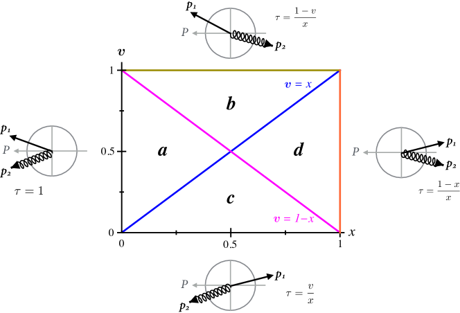
Figure 1: Regions of two-body phase space in the Breit frame. In this frame the incoming proton has momentum along the $-z$ direction given by $P=Q\bar{n}_{z}/(2x)$. The figure shows a quark and a gluon in the final state, corresponding to the Feynman diagrams in Fig. 7. For the diagrams in Fig. 8 there would be a quark and an antiquark in the final state. The 1-jettiness $\tau$ groups particles into back-to-back hemispheres in this frame, in the $\pm z$ directions. There are four distinct regions in $x$ and $v\equiv p_{2}^{-}/Q$ space in which the particles are grouped differently, making $\tau$ a function $\tau(x,v)$. In regions (a) and (d) both particles end up in the same region, giving a constant value of $\tau$. In regions (b) and (c) the two particles are in opposite regions, and $\tau$ varies according to the projection of the two particles’ momenta onto the $\pm z$ axes. The values of $\tau$ in these four regions are given in Eq. (38), and enter the phase space integral in Eq. (36).

We find it convenient to rewrite the phase space in Eq. (34) in terms of a dimensionless variable $v\equiv p_{2}^{-}/Q$,

$$W_{\mu\nu}^{j[2]}=\frac{1}{s_{j}}\frac{1}{8\pi}\Bigl{(}\frac{4\pi}{Q^{2}}\Bigr{)}^{\epsilon}\frac{1}{\Gamma(1-\epsilon)}\bigg{(}\frac{x}{1-x}\bigg{)}^{\epsilon}\,\int_{0}^{1}\frac{dv}{v^{\epsilon}(1-v)^{\epsilon}}\mathcal{M}_{\mu}^{*}\mathcal{M}_{\nu}\delta\Bigl{(}\tau-\tau(x,v)\Bigr{)}\,.$$ (36)

The 1-jettiness $\tau$ is now expressed as a function of $x$ and $v$. Two particles in the final state can be assigned in four different ways to the two hemispheres, and the formula for $\tau(x,v)$ differs in each of these regions. These four regions $(a)$ to $(d)$ are illustrated in Fig. 1. The function $\tau(x,v)$ can be broken down into four pieces,

$$\tau(x,v)=\sum_{i\in\{a,b,c,d\}}\Theta^{(i)}(x,v)\tau^{(i)}(x,v)\,,$$ (37)

where the two-dimensional step function $\Theta^{(i)}$ covers each region $(i)$ and $\tau^{(i)}$ is the value of 1-jettiness in the corresponding region:

$$\tau^{(i)}(x,v)=\begin{cases}1\hskip 56.9055pt\\ \frac{1-v}{x}\\ \frac{v}{x}\\ \frac{1-x}{x}\end{cases}\,,\hskip 28.45274pt\Theta^{(i)}(x,v)=\begin{cases}\theta(-v+(1-x))\,\theta(v-x)\hskip 56.9055pt&i=a\,,\\ \theta(v-(1-x))\,\theta(v-x)\hskip 56.9055pt&i=b\,,\\ \theta(-v+(1-x))\,\theta(-v+x)\hskip 56.9055pt&i=c\,,\\ \theta(v-(1-x))\,\theta(-v+x)\hskip 56.9055pt&i=d\,.\end{cases}$$ (38)

Note that in regions $i=a,d$ the value of $\tau$ is constant in $v$ and thus the delta function comes outside the integral in Eq. (36). As illustrated in Fig. 1, in these two regions both final state particles are in the same hemisphere, and $\tau$ takes the $v$ independent value shown in Eq. (38) over the entire region, which corresponds to the maximum values of $\tau$ given in Eq. (11). In regions $i=b,c$, the value of $\tau$ varies with $v$ and thus the delta function remaining in Eq. (36) can be used to evaluate the $v$ integral.

We evaluate the integral Eq. (36) over the four regions in Fig. 1 using the expressions Eq. (38) in App. B.3.

4 Analytic Results for DIS 1-Jettiness Structure Functions

In this section we present our analytic results for the structure functions in Eq. (2.3) that determine the 1-jettiness cross section in Eq. (17). We will present our results in terms of the structure functions appearing in the cumulative (integrated) cross section,

$$\sigma^{c}(x,Q^{2},\tau)\equiv\int_{0}^{\tau}d\tau^{\prime}\frac{d\sigma}{dx\,dQ^{2}\,d\tau^{\prime}}\,,$$ (39)

which decomposes into structure functions $F_{i}$ exactly like Eq. (17), where

$$F_{i}(x,Q^{2},\tau)=\int^{\tau}_{0}d\tau^{\prime}\,\mathcal{F}_{i}(x,Q^{2},\tau^{\prime})\,,$$ (40)

where the $\mathcal{F}_{i}$ are given by Eq. (2.3). The results for the integrated structure functions $F_{i}$ are more compact to write down than for $\mathcal{F}_{i}$. We give the results for the differential structure functions $\mathcal{F}_{i}$ in App. C.

As the cross section in Eq. (1) is written in terms of singular and nonsingular parts, we express the structure functions as:

$$F_{i} =F_{i}^{\text{sing}}+F_{i}^{\text{ns}}\,.$$ (41)

The fixed-order structure functions are obtained from the calculation of projected hadronic tensors in Eq. (2.3) that are calculated in App. B and App. C. The singular part of the cross section was calculated in Kang:2013nha . Our main new results here are the nonsingular parts of the structure functions that are obtained by subtracting off the known singular parts from the full expressions.

We will present our final expressions for the singular and nonsingular parts of $F_{1}$ and $F_{L}$ in Eq. (41) in the following form:

$$F_{1}(x,Q^{2},\tau) =\sum_{i\in\{q,\bar{q},g\}}(A_{i}+B_{i})\,,$$ (42a)

$$F_{L}(x,Q^{2},\tau) =\sum_{i\in\{q,\bar{q},g\}}4x\,A_{i}\,.$$ (42b)

The singular parts of these can be extracted from the singular cross section in Kang:2013nha , and are given in Eq. (46). Our main new results here are for the nonsingular parts. The functions $A^{\text{ns}}_{i}$ and $B^{\text{ns}}_{i}$ are given by the nonsingular parts of $P^{\mu}P^{\nu}W^{i}_{\mu\nu}$ and $-g^{\mu\nu}W^{i}_{\mu\nu}$, respectively. They are obtained by integrating the differential structure functions in Eq. (92). We find

$$A^{\text{ns}}_{q} =\sum_{f}Q_{f}^{2}\frac{\alpha_{s}C_{F}}{4\pi}\biggl{\{}\Theta_{0}\!\!\int_{x}^{\frac{1}{1+\tau}}dz\,f_{q}(\tfrac{x}{z})(2z\tau-1)+\int_{x}^{1}dz\,f_{q}(\tfrac{x}{z})\biggr{\}}\,,$$ (43a)

$$A^{\text{ns}}_{g} =\sum_{f}Q_{f}^{2}\frac{\alpha_{s}T_{F}}{\pi}\biggl{\{}\Theta_{0}\!\!\int_{x}^{\frac{1}{1+\tau}}dzf_{g}(\tfrac{x}{z})(2z\tau-1)(1-z)+\int_{x}^{1}dz\,f_{g}(\tfrac{x}{z})(1-z)\biggr{\}}\,,$$ (43b)

$$B^{\text{ns}}_{q} =\sum_{f}Q_{f}^{2}\frac{\alpha_{s}C_{F}}{4\pi}\biggl{\{}\Theta_{0}\!\!\int_{x}^{\frac{1}{1+\tau}}\!\!\frac{dz}{z}f_{q}(\tfrac{x}{z})\Bigl{[}\frac{1-4z}{2(1-z)}(2z\tau-1)+P_{qq}(z)\ln\frac{z\tau}{1-z\tau}\Bigr{]}$$

$$\qquad+f_{q}(x)\bigl{(}3\ln\tau+2\ln^{2}\tau\bigr{)}+\int_{x}^{1}\frac{dz}{z}f_{q}(\tfrac{x}{z})\Bigl{[}\mathcal{L}_{0}(1-z)\frac{1-4z}{2}-P_{qq}(z)\ln z\tau\Bigr{]}\biggr{\}}\,,$$ (43c)

$$B^{\text{ns}}_{g} =\sum_{f}Q_{f}^{2}\frac{\alpha_{s}T_{F}}{2\pi}\biggl{\{}\Theta_{0}\!\!\int_{x}^{\frac{1}{1+\tau}}\frac{dz}{z}f_{g}(\tfrac{x}{z})\biggl{[}-(2z\tau-1)+P_{qg}(z)\ln\frac{z\tau}{1-z\tau}\biggr{]}$$

$$\hskip 199.16928pt-\int_{x}^{1}\frac{dz}{z}f_{g}(\tfrac{x}{z})\bigl{[}1+P_{qg}(z)\ln z\tau\bigr{]}\biggr{\}}\,,$$ (43d)

which is one of our main results. Here, we have defined the theta function

$$\Theta_{0}\equiv\Theta_{0}(\tau,x)\equiv\theta(\tau)\theta(1-\tau)\theta\biggl{(}\frac{1-x}{x}-\tau\biggr{)}\,,$$ (44)

which turns on inside the physically-allowed region $0<\tau<\tau^{\text{max}}$ given by Eq. (11) and turns off outside. The plus distribution $\mathcal{L}_{n}(z)$ is defined in App. A. The standard splitting functions $P_{qq}$ and $P_{qg}$ are given by

$$P_{qq}(z) \equiv\left[\theta(1-z)\frac{1+z^{2}}{1-z}\right]_{+}=(1+z^{2})\mathcal{L}_{0}(1-z)+\frac{3}{2}\delta(1-x)$$ (45a)

$$P_{qg}(z) \equiv\theta(1-z)[(1-z)^{2}+z^{2}].$$ (45b)

The formulas for $B_{q}$ and $B_{g}$ in Eqs. (43) and (43) appear to contain terms which are still divergent as $\tau\to 0$, but these divergences cancel in the sum of all terms. Formulas for $B_{q,g}$ given as sums of explicitly nonsingular terms can be found in Eq. (95).

One may recognize that the $\Theta_{0}$ terms in Eq. (43) introduce a discontinuity in the cumulative cross section at $\tau=1$. This feature is associated with asymmetric initial momentum in the $z$ direction, which can give rise to an event with one of the hemispheres containing all final-state particles and the other being empty. As illustrated in Fig. 1, this occurs in regions $(a)$ and $(d)$, where $\tau$ takes on its maximum allowed values in Eq. (11), $1$ for $x<1/2$ and $(1-x)/x$ for $x>1/2$. For $x<1/2$, this appears at $\tau=1$ as a delta function in the differential structure functions Eq. (92) and a discontinuity in the integrated structure functions Eq. (43). However, this feature is not seen for $x>1/2$ at $\tau=(1-x)/x$, because we see that the integrals proportional to $\Theta_{0}$ in Eq. (43) go to zero for $\tau=(1-x)/x$, the range of integration shrinking to zero.

The singular part of the cross section has been computed in Kang:2013nha , from which the singular part of the structure functions can be extracted. $F_{1}^{\text{sing}}$ is simply half of the cumulant cross section given in Eq. (174) in Kang:2013nha , and $F_{L}^{\text{sing}}=0$. The singular parts $A^{\text{sing}}_{i}$ and $B^{\text{sing}}_{i}$ of the functions in Eq. (42) are given by

$$A^{\text{sing}}_{q,g} =0\,,$$ (46a)

$$B^{\text{sing}}_{q} =\sum_{f}Q_{f}^{2}\biggl{\{}f_{q}(x)\bigg{[}\frac{1}{2}-\frac{\alpha_{s}C_{F}}{4\pi}\biggl{(}\frac{9}{2}+\frac{\pi^{2}}{3}+3\ln\tau+2\ln^{2}\tau\biggr{)}\bigg{]}$$

$$\qquad\quad+\frac{\alpha_{s}C_{F}}{4\pi}\int_{x}^{1}\frac{dz}{z}f_{q}(x/z)\biggl{[}\mathcal{L}_{1}(1-z)\,(1+z^{2})+(1-z)+P_{qq}(z)\ln\frac{Q^{2}\tau}{\mu^{2}}\biggr{]}\biggr{\}}\,,$$ (46b)

$$B^{\text{sing}}_{g} =\sum_{f}Q_{f}^{2}\frac{\alpha_{s}T_{F}}{2\pi}\int_{x}^{1}\frac{dz}{z}f_{g}(x/z)\biggl{[}1-P_{qg}(z)+P_{qg}(z)\ln\frac{Q^{2}\tau(1-z)}{\mu^{2}}\biggr{]}\,.$$ (46c)

The sum of Eqs. (43) and (46) gives the complete fixed-order $\mathcal{O}(\alpha_{s})$ result for the DIS 1-jettiness structure functions. When we take values of $\tau$ beyond the physical maximum, where $\Theta_{0}$ terms are turned off, the result reproduces the standard inclusive structure functions in $x$ and $Q^{2}$, which are given by (e.g. Ellis:1991qj )

$$F_{1}(x,Q^{2}) =\sum_{f}Q_{f}^{2}\int_{x}^{1}\frac{dz}{z}\,\biggl{\{}\bigg{[}\frac{\delta(1-z)}{2}+\frac{\alpha_{s}C_{F}}{4\pi}\,C_{q}(z)\bigg{]}\,\bigl{[}f_{q}\bigl{(}\tfrac{x}{z}\bigr{)}+f_{\bar{q}}\bigl{(}\tfrac{x}{z}\bigr{)}\bigr{]}+\frac{\alpha_{s}T_{F}}{2\pi}\,C_{g}(z)f_{g}\bigl{(}\tfrac{x}{z}\bigr{)}\biggr{\}}\,,$$ (47a)

$$F_{L}(x,Q^{2}) =4x\sum_{f}Q_{f}^{2}\int_{x}^{1}dz\,\bigg{\{}\frac{\alpha_{s}C_{F}}{4\pi}\,\bigl{[}f_{q}\bigl{(}\tfrac{x}{z}\bigr{)}+f_{\bar{q}}\bigl{(}\tfrac{x}{z}\bigr{)}\bigr{]}+\frac{\alpha_{s}T_{F}}{\pi}(1-z)\,f_{g}\bigl{(}\tfrac{x}{z}\bigr{)}\bigg{\}}\,,$$ (47b)

where we have defined the two functions

$$C_{q}(z) \equiv-\bigg{(}\frac{9}{2}+\frac{\pi^{2}}{3}\bigg{)}\delta(1-z)-\frac{3}{2}\mathcal{L}_{0}(1-z)+2\mathcal{L}_{1}(1-z)$$ (48a)

$$\hskip 113.81102pt+3-(1+z)\ln(1-z)+P_{qq}(z)\,\ln\frac{Q^{2}}{\mu^{2}\,z}\,,$$

$$C_{g}(z) \equiv 1+P_{qg}(z)\bigg{[}-2+\ln\bigg{(}\frac{Q^{2}}{\mu^{2}}\frac{1-z}{z}\bigg{)}\bigg{]}\,.$$ (48b)

In this section we have presented the complete $\mathcal{O}(\alpha_{s})$ results for the fixed-order structure functions in the DIS 1-jettiness cross section. The expressions Eq. (43) for the nonsingular contributions to the structure functions in Eq. (42) are the primary new results of this paper.

5 Numerical Results

In this section, we present numerical results for the structure functions $\mathcal{F}_{1,L}$ that appear in the differential 1-jettiness cross section in Eq. (17) and the corresponding $F_{1,L}$ in Eq. (40) that appear in the integrated cross section Eq. (39). We computed these structure functions to $\mathcal{O}(\alpha_{s})$ in Sec. 4 and App. C. We also present predictions for the $\tau$ cross sections themselves. For structure functions, we show the fixed-order $\mathcal{O}(\alpha_{s})$ results for the singular part (in $\tau$), the nonsingular part and their sum. For the cross section, we show resummed results at NLL${}^{\prime}+\mathcal{O}(\alpha_{s})$ accuracy as well as the pure fixed-order results. At this order of accuracy we have the fixed-order parts of the hard, jet, beam, and soft functions in the singular part Eq. (101) at the same order in $\mathcal{O}(\alpha_{s})$ as in the nonsingular part.

For our numerical results plotted here, we set the collision energy to be $\sqrt{s}=300\text{ GeV}$, which corresponds to the H1 and ZEUS experiments, and choose $Q=80\text{ GeV}$. We adopt MSTW2008 PDF sets at NLO Martin:2009iq with five light quark and antiquark flavors and run $\alpha_{s}(\mu)$ with the 2-loop beta function in Eq. (105) starting at the values $\alpha_{s}(m_{Z})=0.1202$ used in NLO PDFs.

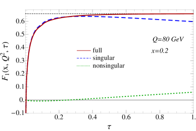
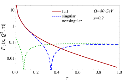
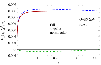
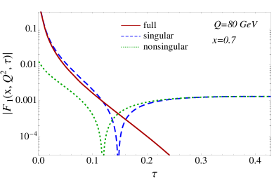
Figure 2: Fixed order components of structure function $F_{1}(x,Q^{2},\tau)$ (left) in the integrated $\tau$ cross section and $\mathcal{F}_{1}(x,Q^{2},\tau)$ (right) in the differential $\tau$ cross section at $Q=80\text{ GeV}$ and $x=0.2$ and 0.7. Full (red solid), singular (blue dashed), and nonsingular (green dotted) contributions. Horizontal dashed line in left plots indicates total $F_{1}(x,Q^{2})$ in Eq. (47a).

Fig. 2 shows the components of the fixed-order results for the structure function $F_{1}(x,Q^{2},\tau)$ in the integrated cross section, given by Eqs. (42a), (43), and (46), and of the $\mathcal{F}_{1}(x,Q^{2},\tau)$ in the differential distribution, given by Eqs. (89), (91), and (92), at two values $x=0.2$ and 0.7. We set all scales to be $\mu=Q=80\text{ GeV}$. In the integrated structure function $F_{1}$, the sum of singular (dashed line) and nonsingular (dotted line) contributions give the full result (solid line). The full result approaches the total result $F_{1}(x,Q^{2})$ (horizontal dashed line) in Eq. (47a) as $\tau$ approaches 1. For $x=0.2$, the singular part alone undershoots the total, and the nonsingular part makes up the difference. For $x=0.7$, the singular part overshoots the total, and the corresponding nonsingular part is mostly negative. Although it is imperceptible in Fig. 2, there is actually a small discontinuity in the $x=0.2$ plot at $\tau=1$, and the total (solid red) $F_{1}$ does not reach the full result (dashed black) until above $\tau=1$. We will zoom in on this feature in Fig. 4.

For the differential $\mathcal{F}_{1}$ in Fig. 2, we plot the absolute value on a log scale. The results illustrate that there is a large cancellation between the singular and nonsingular pieces in the large $\tau$ region so that the total goes to zero in this tail. This same cancellation was discussed for $e^{+}e^{-}$ thrust in Ref. Abbate:2010xh , and appears in various other cross sections that have singular and nonsingular components. The tail falls faster for larger $x$ because $\tau$ dependence enters into PDFs in a form like $f_{q}(x(1+\tau))$, as seen in Eq. (92), which falls faster as $x$ increases. The overall normalization also becomes smaller for larger $x$ due to the PDFs falling off.

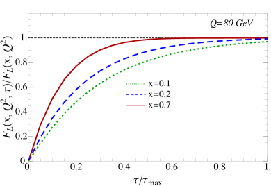
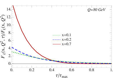
Figure 3: Longitudinal structure function $F_{L}(x,Q^{2},\tau)$ (left) for the integrated $\tau$ cross section and $\mathcal{F}_{L}(x,Q^{2},\tau)$ (right) for the differential $\tau$ cross section, divided by the total $F_{L}(x,Q^{2})$ in Eq. (47b) at $Q=80~{}\text{ GeV}$ and $x=0.1,~{}0.2~{}\text{and},~{}0.7$.

Fig. 3 shows the fixed-order results for the longitudinal structure function $F_{L}(x,Q^{2},\tau)$ for the integrated cross section, given by Eqs. (42b) and (43), and $\mathcal{F}_{L}(x,Q^{2},\tau)$ for the differential distribution, given by Eqs. (89) and (92), at $x=0.1\,,0.2,$ and 0.7. These are purely nonsingular in $\tau$. The plots are normalized to the total $F_{L}(x,Q^{2})$ in Eq. (47b). Note that $\mathcal{F}_{L}$ is finite at $\tau=0$ at $\mathcal{O}(\alpha_{s})$. The distribution monotonically decreases with $\tau$. For the left plot at $x=0.1,0.2$, there is a perceptible gap from the total (straight dashed line) at $\tau=1$ before the curves reach the value 1. This jump is explored in Fig. 4.

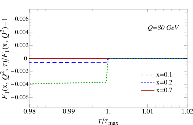
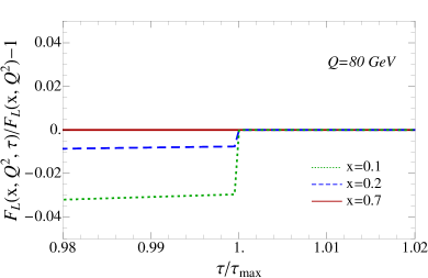
Figure 4: Discontinuities of normalized cumulants $F_{1}$ and $F_{L}$ at $Q=80\text{ GeV}$ and $x=0.1,\,0.2,\,0.7$.

Fig. 4 illustrates the discontinuities in the cumulative $F_{1}$ and $F_{L}$ near $\tau^{\text{max}}$. The jump is smaller than 1% in $F_{1}$ and is about a few percent in $F_{L}$. These discontinuities are reduced for increasing $x$ and disappear at $x=1/2$ and beyond. As described in Sec. 4, these discontinuities are associated with events where the jet hemisphere is empty and the beam hemisphere contains all final-state particles as seen in the Breit frame, so whole regions of phase space end up contributing to the same fixed value of $\tau$ (see Fig. 1). Such events do not occur in the observables defined in the partonic CM frame such as $e^{+}e^{-}$ thrust. This discontinuity is infrared safe, and though its magnitude is very small, it is in principle measurable.

The cross section in Eq. (1) with all the scale dependencies made explicit in singular and nonsingular parts can be written

$$\sigma^{\text{full}}(\tau;\mu_{H},\mu_{J},\mu_{B},\mu_{S},\mu_{\text{ns}})=\sigma^{\text{sing}}(\tau;\mu_{H},\mu_{J},\mu_{B},\mu_{S})+\sigma^{\text{ns}}(\tau;\mu_{\text{ns}})\,,$$ (49)

and is given in Eq. (101). The singular part depends on the scales $\mu_{H}$, $\mu_{J}$, $\mu_{B}$, $\mu_{S}$ associated with hard, jet, beam, and soft radiation, respectively, and the nonsingular part depends on $\mu_{\text{ns}}$ as in conventional fixed-order results. For the full calculation, all scales should be specified. In the region $\tau\ll 1$, there are large logarithms in the singular part and the logarithms can be resummed by RG evolution of the functions between $\mu$ and their individual canonical scales: $\mu_{H}\sim Q$, $\mu_{B,J}\sim\sqrt{\tau}Q$, $\mu_{S}\sim\tau Q$. (For more details on resummation of the singular part, see Kang:2013nha . Basic results are reviewed in App. E.) However, $\mu_{S}$ cannot be arbitrary small and it should freeze above the nonperturbative regime that lives below $1$ GeV. On the opposite end, where $\tau\sim\mathcal{O}(1)$ and logs of $\tau$ are not large, the resummation should be turned off by setting all $\mu_{i}\approx Q$. In Kang:2013nha we used profile functions $\mu_{i}(\tau)$ satisfying above constraints and estimated perturbative uncertainties by varying parameters in the profile functions Ligeti:2008ac ; Abbate:2010xh ; Berger:2010xi . However, the profile defined in Kang:2013nha has scales away from the canonical scales when $x$ increases. Here we use improved profiles given in App. D, which set canonical scales in the resummation region that are independent of $x$. Fig. 5 shows the soft scale $\mu_{S}(\tau)$ as a function of $\tau$ at $x=0.2$ and $0.7$ as well as the canonical choice $\tau Q$ (dashed line).

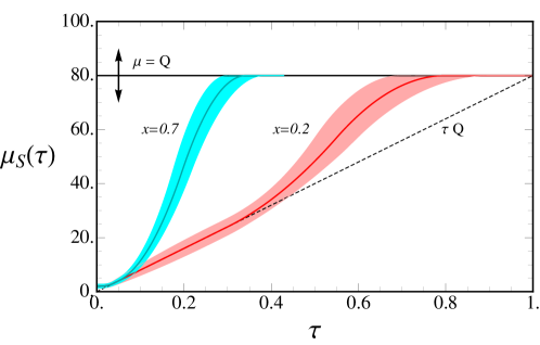
Figure 5: Profile $\mu_{S}(\tau)$ for $x=0.2$ and $0.7$ for $Q=80\text{ GeV}$. Uncertainty bands are sum of all variations in Eq. (100) in quadrature. The dashed line indicates the canonical choice $\mu_{s}(\tau)=\tau Q$ and the vertical arrow implies that the scale $\mu$ is varied up and down by a factor of 2.

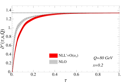
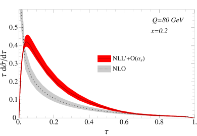
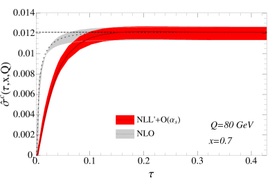
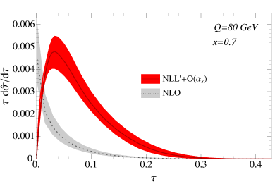
Figure 6: Cumulant and differential cross section at NLL${}^{\prime}+\mathcal{O}(\alpha_{s})$ for $Q=80\text{ GeV}$ and $x=0.2$ and 0.7. The uncertainty bands for the resummed results are obtained by summing all scale variations described in Eqs. (50) and (100) in quadrature.

For the central values of $\mu_{\text{ns}}$ and its variations, we make the same choice as Abbate:2010xh ,

$$\mu_{\text{ns}} =\mu_{J}\,, \mu_{\text{ns}} =\Big{[}\frac{\mu_{J}+\mu_{s}}{2},\mu_{H}\Big{]}\,.$$ (50)

The scales are chosen to estimate theory uncertainties from un-resummed subleading logarithms in the nonsingular part.

Fig. 6 shows resummed integrated and differential cross sections at NLL${}^{\prime}+\mathcal{O}(\alpha_{s})$ as well as the purely fixed-order result at $\mathcal{O}(\alpha_{s})$. We plot normalized cross sections defined as

$$\hat{\sigma}^{c}(x,Q^{2},\tau)=\frac{\sigma^{c}(x,Q^{2},\tau)}{\sigma_{0}}\,,\qquad\tau\frac{d\hat{\sigma}}{d\tau}=\frac{\tau}{\sigma_{0}}\,\frac{d\sigma}{dx\,dQ^{2}\,d\tau}\,.$$ (51)

where $\sigma_{0}=2\pi\alpha^{2}[1+(1-y)^{2}]/Q^{4}$. We multiply the differential distribution by $\tau$ for ease of displaying the whole $\tau$ region.

The uncertainty bands for the resummed results are obtained by summing all scale variations described in Eqs. (50) and (100) in quadrature. The uncertainty bands for the fixed-order results are obtained from varying the central scale $\mu=Q$ up and down by factors of 2. As seen in Fig. 2 the tail of the distribution becomes shorter with increasing $x$. Relative uncertainties about the central value are larger for larger $x$ because of slower convergence of the perturbative corrections associated with the PDF for increasing $x$ (as can be seen from the fact that the residual scale dependence of the PDF increases with $x$).

Fig. 6 only includes purely perturbative results. Nonperturbative effects in 1-jettiness are power suppressed by $\Lambda_{\text{QCD}}/(\tau Q)$ for $\tau\gg\Lambda_{\text{QCD}}/Q$, and the leading power correction can be expressed in terms of a single nonperturbative parameter $\Omega_{1}$. The parameter is universal for different versions of 1-jettiness in DIS defined in Kang:2013nha , and even appears in the power corrections for certain jet observables in $pp\to H/Z+\text{jet}$ with a small jet radius Stewart:2014nna . Alternatively, a shape function that takes nonperturbative behavior into account in the nonperturbative region as well as the power correction region Hoang:2007vb , can be used as in Kang:2013nha . In this paper, we omit implementing these nonperturbative effects.

6 Conclusions

Events with one or more jets plus initial state radiation dominate the population of final states in DIS for typical values of $x$. These events can be further probed by the inclusive event shape 1-jettiness $\tau$. Events with small values of $\tau$ contain only one non-ISR jet, while multiple jets populate the large $\tau$ region. In this paper, we obtained analytically the $\mathcal{O}(\alpha_{s})$ cross section for all values of $\tau$, and combined it with NLL^′ resummation of the singular terms at small $\tau$ to obtain results accurate over the entire range of $\tau$. This is the first analytic calculation of a DIS event shape at this order.

We wrote the results in terms of structure functions $F_{1}(x,Q^{2},\tau)$ and $F_{L}(x,Q^{2},\tau)$ which generalize the usual DIS structure functions $F_{1,L}(x,Q^{2})$. We gave structure functions for both the cumulative or integrated $\tau$ distribution as well as the differential $\tau$ distribution. Our predictions for the cumulative distribution agree with the total $F_{1,L}(x,Q^{2})$ for $\tau>\tau^{\text{max}}$.

The cumulative cross section displays an interesting feature, a small discontinuity at $\tau=1$, which is a consequence of asymmetric initial momentum that can lead to one of hemispheres (in the Breit frame) being empty in the final state. This does not happen in $e^{+}e^{-}$ thrust defined in the partonic CM frame.

We presented numerical results with perturbative uncertainties by varying scales at the HERA energy. In general the uncertainties grow with $x$ due to the convergence of perturbative corrections in the cross section that are connected with the PDFs through their scale dependence. The tail of the $\tau$ distribution falls off faster as $x$ grows. The size of the nonsingular terms is consistent with our expectations from Kang:2013nha where we compared the resummed singular cross section with the total QCD cross section at $x,Q^{2}$.

Our results represent a significant improvement in precision in the prediction of DIS event shape cross sections. The groundwork is in place to go to higher resummed N3LL and fixed-order accuracy which we will pursue in the near future, and bring the science of event shapes in DIS to the same level of precision as has been achieved in $e^{+}e^{-}$. These predictions can be tested with existing HERA data and future EIC data, which should yield determinations of the strong coupling and hadron structure to unprecedented accuracy.

Appendix A Plus Distributions

In this section, we define plus distributions that we use and collect some useful identities involving them. The standard set of plus distributions $\mathcal{L}_{n}(z)$ are defined by (see, e.g., Ligeti:2008ac )

$$\mathcal{L}_{n}(z)\equiv\lim_{\varepsilon\to 0}\frac{d}{dz}\bigg{[}\frac{\theta(z-\varepsilon)\ln^{n+1}z}{n+1}\bigg{]}=\bigg{[}\frac{\theta(z)\ln^{n}(z)}{z}\bigg{]}_{+}\,.$$ (52)

Integrating against a well-behaved test function $g(z)$ gives the familiar rule,

$$\int^{z}_{0}dz^{\prime}\mathcal{L}_{n}(z^{\prime})g(z^{\prime})=\int^{z}_{0}dz^{\prime}\frac{\ln^{n}z^{\prime}}{z^{\prime}}[g(z^{\prime})-g(0)]+g(0)\frac{\ln^{n+1}z}{n+1}.$$ (53)

We also define a distribution function with two arguments, which can be used when the presence of the divergence in a variable $z$ is controlled by the value of a second variable $z_{0}$,

$$\mathcal{L}_{n}(z,z_{0}) \equiv\lim_{\varepsilon\to 0}\frac{d}{dz}\bigg{[}\frac{\theta(z-z_{0}-\varepsilon)\ln^{n+1}z}{n+1}\bigg{]}\hskip 56.9055ptz_{0}\geq 0\,,$$ (54)

$$\int_{0}^{z}dz^{\prime}\mathcal{L}_{n}(z^{\prime},z_{0})g(z^{\prime}) =\int^{z}_{z_{0}}dz^{\prime}\,\frac{\ln^{n}z^{\prime}}{z^{\prime}}[g(z^{\prime})-g(z_{0})]+g(z_{0})\frac{\ln^{n+1}z}{n+1}\,,$$ (55)

where $g(z)$ is a test function. In the standard distribution $\mathcal{L}_{n}(z)$ the subtraction of the singularity occurs at the singular point $z=0$, while in $\mathcal{L}(z,z_{0})$ the subtraction occurs at $z=z_{0}$ even if there is no singularity when $z_{0}\neq 0$. $\mathcal{L}(z,z_{0})$ reduces to $\mathcal{L}(z)$ at $z_{0}=0$.

Evaluating phase space or loop integrals at $\mathcal{O}(\alpha_{s})$ or higher in dimensional regularization, we encounter singular terms like

$$\frac{\theta(z)}{z^{1+\epsilon}} =-\frac{\delta(z)}{\epsilon}+\mathcal{L}_{0}(z)-\epsilon\mathcal{L}_{1}(z)+\mathcal{O}(\epsilon^{2})\,,$$ (56)

which have been expanded in powers of $\epsilon$ making use of the plus distributions in Eq. (52). We also encounter more complicated doubly-singular expressions, e.g. in Eqs. (76) and (78), which can be expanded in $\epsilon$ using both Eqs. (52) and (54), such as:

$$\frac{\theta(\tau)}{\tau^{1+\epsilon}}\frac{\theta\big{(}z-\tfrac{\tau}{1+\tau}\big{)}}{z^{1+\epsilon}}=\frac{\delta(z)\delta(\tau)}{2\epsilon^{2}}-\frac{\delta(\tau)\mathcal{L}_{0}(z)}{\epsilon}+I^{s}(\tau,z)+I^{\text{ns}}(\tau,z)+\mathcal{O}(\epsilon)\,,$$ (57)

where the ${\cal O}(\epsilon^{0})$ terms are

$$I^{s}(\tau,z)=\delta(\tau)\mathcal{L}_{1}(z)+\mathcal{L}_{0}(z)\mathcal{L}_{0}(\tau)-\mathcal{L}_{1}(\tau)\delta(z)\,,$$ (58)

$$I^{\text{ns}}(\tau,z)=-\big{[}\delta\big{(}z-\tfrac{\tau}{1+\tau}\big{)}-\delta(z)\big{]}\frac{\theta(\tau)\ln\tau}{\tau}+\big{[}\mathcal{L}_{0}\big{(}z,\tfrac{\tau}{1+\tau}\big{)}-\mathcal{L}_{0}(z)\big{]}\frac{\theta(\tau)}{\tau}+\delta\big{(}z-\tfrac{\tau}{1+\tau}\big{)}\frac{\ln(1+\tau)}{\tau}$$

$$\hskip 56.9055pt-\frac{\delta^{\prime}\big{(}-\tau+\tfrac{z}{1-z}\big{)}}{(1-z)^{2}}\theta(\tau)\bigg{[}-\operatorname{Li}(z)+\operatorname{Li}\Big{(}\frac{\tau}{1+\tau}\Big{)}+\frac{\ln^{2}(1+\tau)}{2}-\frac{\ln^{2}(z/\tau)}{2}\bigg{]}\,,$$ (59)

where $\operatorname{Li}(z)$ is the dilogarithm, defined by

$$\operatorname{Li}(z)=-\int_{0}^{z}dz^{\prime}\frac{\ln(1-z^{\prime})}{z^{\prime}}\,.$$ (60)

The function $I^{s}(\tau,z)$ is singular both in $\tau$ and $z$, depending on both ${\cal L}(\tau)$ and ${\cal L}(x)$, while $I^{\text{ns}}(\tau,z)$ is not singular in $\tau$ (though still singular in $z$). Note that the term on the last line of Eq. (59), which has a $\delta^{\prime}\big{(}-\tau+\tfrac{z}{1-z}\big{)}$, will not contribute to any of our perturbative structure functions because the expression in brackets that it multiplies and its derivative respect to $\tau$ are both zero at $\tau=\tfrac{z}{1-z}$.

Appendix B Hadronic Tensor at Parton Level

In this section we calculate the hadronic tensor $W_{\mu\nu}$ defined in Eq. (14) where the proton initial state is replaced with a partonic (quark or gluon) state. Such a computation allows us to extract the short-distance matching coefficients $w_{\mu\nu}^{q,g}$ in Eq. (19) onto PDFs, as described in Sec. 3.1. We denote the tensor for a quark initial state as $W^{q}_{\mu\nu}$ and for a gluon initial state as $W^{g}_{\mu\nu}$. Up to $\mathcal{O}(\alpha_{s})$, $W^{q}_{\mu\nu}$ involves a tree-level contribution and the one-gluon diagrams in Fig. 7, and can be decomposed into

$$W^{q}_{\mu\nu}=W_{\mu\nu}^{(0)}+W_{\mu\nu}^{\text{vir}}+W_{\mu\nu}^{\text{real}}\,.$$ (61)

Meanwhile, $W^{g}_{\mu\nu}$ is given just by tree-level real diagrams at $\mathcal{O}(\alpha_{s})$, shown in Fig. 8.

The partonic tensor $W_{\mu\nu}^{i}$ can be computed from Eq. (30), which is a phase space integral over the squared amplitude. In this section we compute the squared amplitudes; in the next section we will evaluate the complete phase space integrals. Figs. 7 and 8 represent the $\mathcal{O}(\alpha_{s})$ amplitudes for initial quark and initial gluon states. In App. B.1 and App. B.2 we evaluate the squared amplitudes built from these diagrams. The real diagrams have two-body final states with momenta $p_{1}$ and $p_{2}$ and as described in Fig. 1, they can enter two back-to-back hemispheres in four different ways, and the formula for the 1-jettiness $\tau$ in terms of $p_{1,2}$ in each configuration differs.

B.1 Squared Amplitudes for $\gamma^{*}+q$

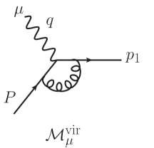
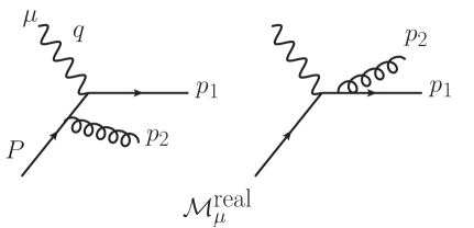
Figure 7: Virtual and real diagrams for $\gamma^{*}+\text{quark}$ processes at $\mathcal{O}(\alpha_{s})$. They contribute to the virtual amplitudes in Eqs. (B.1) and (65) and the real amplitudes in Eqs. (B.1) and (68). There are also corresponding diagrams for incoming antiquarks.

For the process $\gamma^{*}(q^{\mu})+q(P^{\mu})\to q(p_{1}^{\mu})$ at tree level, the amplitude is $\bar{u}(p_{1})\gamma_{\mu}u(P)$. To obtain the structure functions Eq. (2.3) one needs projected squared amplitudes as

$$-g^{\mu\nu}\,\mathcal{M}^{(0)}_{\mu}\mathcal{M}^{(0)\,*}_{\nu} =4Q_{f}^{2}\,Q^{2}\,,$$ (62)

$$P^{\mu}P^{\nu}\,\mathcal{M}^{(0)}_{\mu}\mathcal{M}^{(0)\,*}_{\nu} =0\,,$$ (63)

where we have also summed over all quark spins. The projection in Eq. (63) is zero because of the Dirac equation $P\!\!\!\!/\,u(P)=0$. Here, $Q_{f}$ is the electromagnetic charge of quark with flavor $f$. We do not sum over flavors for the quark tensors until we convolve with PDFs.

The virtual contribution can be extracted from the literature, see, e.g., Eq. (14.19) in Sterman:1994ce . At $\mathcal{O}(\alpha_{s})$ we obtain the cross terms between the tree-level and the virtual diagram shown in Fig. 7:

$$-g^{\mu\nu}\,\big{[}\mathcal{M}^{\text{vir}}_{\mu}\mathcal{M}^{(0)\,*}_{\nu}+\mathcal{M}^{(0)}_{\mu}\mathcal{M}^{\text{vir}\,*}_{\nu}\big{]}$$

$$\hskip 28.45274pt=-8Q^{2}\frac{\alpha_{s}C_{F}Q_{f}^{2}}{2\pi}(1-\epsilon)\bigg{(}\frac{4\pi\mu^{2}}{Q^{2}}\bigg{)}^{\epsilon}\frac{\Gamma(1+\epsilon)\Gamma(1-\epsilon)^{2}}{\Gamma(1-2\epsilon)}\bigg{(}\frac{1}{\epsilon^{2}}+\frac{3}{2\epsilon}+4\bigg{)}\,,$$

$$\hskip 28.45274pt=4Q^{2}\frac{\alpha_{s}C_{F}Q_{f}^{2}}{2\pi}(1-\epsilon)\bigg{[}-\frac{2}{\epsilon^{2}}-\frac{1}{\epsilon}\bigg{(}2\ln\frac{\mu^{2}}{Q^{2}}+3\bigg{)}-\ln^{2}\frac{\mu^{2}}{Q^{2}}-3\ln\frac{\mu^{2}}{Q^{2}}+\frac{\pi^{2}}{6}-8\bigg{]}\,,$$ (64)

$$P^{\mu}P^{\nu}\,\big{[}\mathcal{M}^{\text{vir}}_{\mu}\mathcal{M}^{(0)\,*}_{\nu}+\mathcal{M}^{(0)}_{\mu}\mathcal{M}^{\text{vir}\,*}_{\nu}\big{]}=0\,,$$ (65)

again summed over all quark spins. We have kept the factor $(1-\epsilon)$ out front because it is to be cancelled by the same factor in Eq. (2.3). In the second step of Eq. (B.1), we converted to the $\overline{\text{MS}}$ scheme, making the replacement:

$$\mu^{2}\to\frac{\mu^{2}e^{\gamma_{E}}}{4\pi}\,.$$ (66)

Note that the finite part in Eq. (B.1) is the $\alpha_{s}$ term of the hard function, which already appeared in our discussion in Ref. Kang:2013nha . For discussion of the hard function in SCET see Bauer:2003di ; Manohar:2003vb . Eq. (65) is zero again by the Dirac equation $P\!\!\!\!/\,u(P)=0$.

The real contribution to $W_{\mu\nu}^{q}$ in Eq. (61) at $\mathcal{O}(\alpha_{s})$ comes from two diagrams for $\gamma^{*}(q^{\mu})+q(P^{\mu})\to q(p_{1}^{\mu})+g(p_{2}^{\mu})$ shown in Fig. 7. The projected amplitudes for the diagrams, summed over quark spins and gluon polarizations, are given by

$$-g^{\mu\nu}\mathcal{M}_{\mu}^{\text{real}}\mathcal{M}_{\nu}^{\text{real}\,*} =32\pi\alpha_{s}C_{F}Q_{f}^{2}(1-\epsilon)\bigg{(}\frac{\mu^{2}e^{\gamma_{E}}}{4\pi}\bigg{)}^{\epsilon}$$

$$\hskip 56.9055pt\times\bigg{[}(1-\epsilon)\bigg{(}\frac{1-x}{v}+\frac{v}{1-x}\bigg{)}+2\frac{x}{1-x}\frac{1-v}{v}+2\epsilon\bigg{]}\,,$$ (67)

$$P^{\mu}P^{\nu}\,\mathcal{M}_{\mu}^{\text{real}}\mathcal{M}_{\nu}^{\text{real}\,*} =16\pi\alpha_{s}C_{F}Q_{f}^{2}Q^{2}(1-\epsilon)\bigg{(}\frac{\mu^{2}e^{\gamma_{E}}}{4\pi}\bigg{)}^{\epsilon}\frac{1-v}{x}\,,$$ (68)

where $v=p_{2}^{-}/Q$ as in Eq. (36) or Fig. 1. Eq. (B.1) can be found from Eq. (14.23) in Sterman:1994ce .

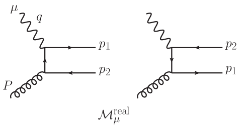
Figure 8: Diagrams for $\gamma^{*}+\text{gluon}$ processes at $\mathcal{O}(\alpha_{s})$. They contribute to the real amplitudes in Eqs. (B.2) and (70). We sum the two diagrams that are related by interchanging the quark and antiquark to obtain Eqs. (B.2) and (70), thus it is necessary only to sum over the five light flavors $u,d,s,c,b$ once, not twice.

B.2 Squared Amplitudes for $\gamma^{*}+g$

The tree-level process with an initial gluon $\gamma^{*}(q^{\mu})+g(P^{\mu})\to q(p_{1}^{\mu})\,\bar{q}(p_{2}^{\mu})$ starts at $\mathcal{O}(\alpha_{s})$, illustrated in Fig. 8. The projected amplitudes for the process, summed over gluon polarizations and quark spins, are given by

$$-g^{\mu\nu}\mathcal{M}_{\mu}^{\text{real}}\mathcal{M}_{\nu}^{\text{real}\,*} =32\pi\alpha_{s}T_{F}\sum_{f}Q_{f}^{2}(1-\epsilon)\bigg{(}\frac{\mu^{2}e^{\gamma_{E}}}{4\pi}\bigg{)}^{\epsilon}$$

$$\hskip 56.9055pt\times\bigg{[}(1-\epsilon)\bigg{(}\frac{1-v}{v}+\frac{v}{1-v}\bigg{)}-2\frac{x(1-x)}{v(1-v)}-2\epsilon\bigg{]}\,,$$ (69)

$$P^{\mu}P^{\nu}\,\mathcal{M}_{\mu}^{\text{real}}\mathcal{M}_{\nu}^{\text{real}\,*} =32\pi\alpha_{s}T_{F}\sum_{f}Q_{f}^{2}Q^{2}(1-\epsilon)\bigg{(}\frac{\mu^{2}e^{\gamma_{E}}}{4\pi}\bigg{)}^{\epsilon}\frac{1-x}{x}\,.$$ (70)

Note that these are symmetric under $v\to 1-v$, which just switches the final-state quark and antiquark in Fig. 8. Note also that the projection in Eq. (70) is independent of $v$, making the phase-space integral in Eq. (36) particularly simple. Here we go ahead and include the sum over quark flavors $f\in\{u,d,s,c,b\}$ since the gluon PDF with which we will convolve these results is independent of quark flavors produced in the final states in Fig. 8. Since both possibilities of the photon interacting with the quark or the antiquark are already included in the sum of the two diagrams in Fig. 8, we need sum over the five light flavors only once, and not repeat the sum for antiquark flavors $\bar{f}$.

B.3 Projected Hadronic Tensor

In this subsection we obtain hadronic tensors by integrating the squared amplitudes obtained in App. B.1 and App. B.2 using the phase space integrations in Eqs. (33) and (36). The latter goes over the four regions in Fig. 1 with a different formula for $\tau(x,v)$ depending on which hemispheres the two final-state particles enter.

B.3.1 Quark tensor

For $P^{\mu}P^{\nu}\,W^{q}_{\mu\nu}$, only the real emission contribution Eq. (68) is nonzero, and it contains no IR divergence, so we can safely set $\epsilon=0$. Using Eq. (36) to integrate Eq. (68) over the four regions in Fig. 1, we obtain the contributions

$$P^{\mu}P^{\nu}W_{\mu\nu}^{(a)} =\alpha_{s}C_{F}Q_{f}^{2}Q^{2}\frac{1-2x}{2x}\theta\Bigl{(}\frac{1}{2}-x\Bigr{)}\delta(\tau-1)\,,$$ (71a)

$$P^{\mu}P^{\nu}W_{\mu\nu}^{(b)} =\alpha_{s}C_{F}Q_{f}^{2}Q^{2}x\tau\,\Theta_{0}(\tau,x)\,,$$ (71b)

$$P^{\mu}P^{\nu}W_{\mu\nu}^{(c)} =\alpha_{s}C_{F}Q_{f}^{2}Q^{2}(1-x\tau)\,\Theta_{0}(\tau,x)\,,$$ (71c)

$$P^{\mu}P^{\nu}W_{\mu\nu}^{(d)} =\alpha_{s}C_{F}Q_{f}^{2}Q^{2}\frac{2x-1}{2x}\theta\Bigl{(}x-\frac{1}{2}\Bigr{)}\delta\Bigl{(}\tau-\frac{1-x}{x}\Bigr{)}\,,$$ (71d)

where the generalized theta function $\Theta_{0}$ is defined in Eq. (44). The sum of the four contributions in Eq. (71) gives the result:

$$P^{\mu}P^{\nu}\,W^{q}_{\mu\nu}=\alpha_{s}C_{F}Q_{f}^{2}\,w_{P}^{q}\,,$$ (72a)

$$w_{P}^{q}=Q^{2}\,\Theta_{0}(\tau,x)\left[1+\delta\Bigl{(}\frac{1}{1+\tau}-x\Bigr{)}\frac{1-\tau}{2(1+\tau)^{2}}+\delta(\tau-1)\frac{1-2x}{2x}\right]\,,$$ (72b)

where in the middle term of Eq. (72b) we rescaled variables in the delta function in Eq. (71d). This result gives the matching coefficient $w_{P}^{q}$ in Eq. (29).

The tree-level and virtual contributions to $-g^{\mu\nu}\,W_{\mu\nu}^{q}$ are given by inserting Eqs. (62) and (B.1) into the formula for a one-body final-state phase space in Eq. (33):

$$\begin{split}-g^{\mu\nu}(W_{\mu\nu}^{(0)}+W_{\mu\nu}^{\text{vir}})&=\biggl{\{}4\pi Q_{f}^{2}+2\alpha_{s}C_{F}Q_{f}^{2}(1-\epsilon)\biggl{[}-\frac{2}{\epsilon^{2}}-\frac{1}{\epsilon}\bigg{(}2\ln\frac{\mu^{2}}{Q^{2}}+3\bigg{)}\\ &\hskip 85.35826pt-\ln^{2}\frac{\mu^{2}}{Q^{2}}-3\ln\frac{\mu^{2}}{Q^{2}}+\frac{\pi^{2}}{6}-8\biggr{]}\biggr{\}}\delta(1-x)\delta(\tau)\,.\end{split}$$ (73)

The contribution from the real diagrams in Eq. (B.1) is more involved. We must integrate Eq. (B.1) over the two-body phase space using Eq. (36). We consider in turn the four contributions $-g^{\mu\nu}\,W_{\mu\nu}^{\text{real}\,(a,b,c,d)}$ corresponding to the four regions in Fig. 1.

In region $(a)$, where $x<v<1-x$ and $x<1/2$, the integrand in Eq. (B.1) is finite and we can set $\epsilon=0$ in Eqs. (36) and (B.1), giving

$$-g^{\mu\nu}\,W_{\mu\nu}^{\text{real}\,(a)} =2\alpha_{s}C_{F}Q_{f}^{2}\,\delta(\tau-1)\,\theta\Bigl{(}\frac{1}{2}-x\Bigr{)}\bigg{[}\frac{(1-2x)(1-4x)}{2(1-x)}+\frac{1+x^{2}}{1-x}\ln\frac{1-x}{x}\bigg{]}\,.$$ (74)

In region $(b)$, $v>x$ and $v>1-x$ and $v=1-x\tau$. Because the $\Theta_{0}(\tau,x)$ in Eq. (44) sets $x<1/(1+\tau)$ the term $1/(1-x)$ in Eq. (B.1) is finite for the region of $x$. So, $\epsilon$ can be set to zero in Eqs. (B.1) and (36) and we have

$$-g^{\mu\nu}\,W_{\mu\nu}^{\text{real}\,(b)} =2\alpha_{s}C_{F}Q_{f}^{2}\Theta_{0}(\tau,x)\,x\bigg{(}\frac{1-x}{1-x\tau}+\frac{1-x\tau}{1-x}+2\frac{x^{2}}{1-x}\frac{\tau}{1-x\tau}\bigg{)}\,.$$ (75)

In region $(c)$, where $v<x$ and $v<1-x$ and $v=x\tau$, there are two IR divergent terms in Eq. (B.1) that go like $1/\tau$ and $1/[\tau(1-x)]$, which can be expanded by using the identities in Eqs. (56) and (57). Then, we have

$$-g^{\mu\nu}\,W_{\mu\nu}^{\text{real}\,(c)} =2\alpha_{s}C_{F}Q_{f}^{2}\bigg{(}\frac{\mu^{2}}{Q^{2}}\bigg{)}^{\epsilon}(1-\epsilon)\Theta_{0}(\tau,x)$$

$$\quad\times\bigg{[}\bigg{(}\frac{1}{\epsilon^{2}}+\frac{3}{2\epsilon}\bigg{)}\delta(\tau)\delta(1-x)-\frac{\delta(\tau)P_{qq}(x)}{\epsilon}+E^{s}(\tau,x)+E^{\text{ns}}(\tau,x)\bigg{]}\,,$$ (76)

where we converted to the $\overline{\text{MS}}$ scheme using Eq. (66), and the singular and nonsingular parts of the finite terms are given by

$$E^{s}(\tau,x) =-2\mathcal{L}_{1}(\tau)\delta(1-x)+\mathcal{L}_{0}(\tau)[P_{qq}(x)-\frac{3}{2}\delta(1-x)]$$

$$\qquad+\delta(\tau)\bigg{[}(1+x^{2})\mathcal{L}_{1}(1-x)-\frac{\pi^{2}}{12}\delta(1-x)+1-x\bigg{]}\,,$$ (77)

$$E^{\text{ns}}(\tau,x) =-(2-\tau)\frac{x^{2}}{1-x}+2x\,I^{\text{ns}}(\tau,1-x)\,,$$ (78)

where $\mathcal{L}_{n}$ and $I^{\text{ns}}(\tau,1-x)$ are given above in Eqs. (52) and (59). The splitting function $P_{qq}(x)$ is given by Eq. (45).

In region $(d)$, where $1-x<v<x$ and $\tau=(1-x)/x$, the term $1/(1-x)$ in Eq. (B.1) is IR divergent because the condition $\Theta_{0}(\tau,x)$ becomes $\theta(x-1/2)\theta(1-x)$. Integrating Eq. (B.1) by using Eq. (36) and expanding in $\epsilon$ by using Eq. (56), we obtain in $\overline{\text{MS}}$,

$$-g^{\mu\nu}\,W_{\mu\nu}^{\text{real}\,(d)}=2\alpha_{s}C_{F}Q_{f}^{2}(1-\epsilon)\bigg{(}\frac{\mu^{2}}{Q^{2}}\bigg{)}^{\epsilon}\delta\bigg{(}\frac{1}{1+\tau}-x\bigg{)}\theta(x-1/2)\,$$ (79)

$$\quad\times\bigg{[}\delta(\tau)\bigg{(}\frac{1}{\epsilon^{2}}+\frac{3}{2\epsilon}+\frac{7}{2}-\frac{5\pi^{2}}{12}\bigg{)}-\frac{3}{2}\mathcal{L}_{0}(\tau)-2\mathcal{L}_{1}(\tau)+\frac{(3\tau^{2}+8\tau+13)+2(2\tau^{2}+5\tau+4)\ln\tau}{2(1+\tau)^{3}}\bigg{]}\,.$$

Now we collect all pieces contributing to $-g_{\mu\nu}W_{\mu\nu}^{q}$ and sum them together. The IR divergent $1/\epsilon^{2}$ and $1/\epsilon$ terms appear with $\delta(1-x)\delta(\tau)$ which are all canceled when the virtual part from Eq. (73) and real parts in Eqs. (76) and (79) are added together. There is one additional IR divergence with $P_{qq}(x)\delta(\tau)/\epsilon$ that is associated with the one-loop quark PDF, and hence remains uncancelled when adding virtual and real contributions. Summing all the terms in Eqs. (74), (75), (76), and (79) together with the tree-level and virtual contributions from Eq. (73), we obtain the final result

$$-g^{\mu\nu}\,W^{q}_{\mu\nu}=4\pi Q_{f}^{2}\delta(1-x)\delta(\tau)+2\alpha_{s}C_{F}Q_{f}^{2}(1-\epsilon)\bigg{[}-\frac{P_{qq}(x)}{\epsilon}\delta(\tau)+w_{G}^{q}\bigg{]}\,,$$ (80a)

$$w_{G}^{q}=\Theta_{0}(\tau,x)\bigg{[}\delta(\tau)\,S_{-1}^{q}(x)+\mathcal{L}_{0}(\tau)\,S_{0}^{q}(\tau,x)+\mathcal{L}_{1}(\tau)\,S_{1}^{q}(\tau,x)$$

$$\hskip 85.35826pt+R^{q}(\tau,x)+\delta(\tau-1)\,\Delta_{1}^{q}(x)+\delta(\tfrac{1}{1+\tau}-x)\,\Delta_{2}^{q}(\tau)\bigg{]}\,.$$ (80b)

Here we separately write IR divergent and finite terms in Eq. (80a) in order to clearly show the structure of the result, which we anticipated above in Eq. (25). From this result we extract the matching coefficient $w_{G}^{q}$ in Eq. (29). The functions $S_{i}^{q}$ are coefficients of singular terms in $\tau$, $R^{q}$ is regular in $\tau$, and $\Delta_{i}$ are coefficients of delta functions. They are given by

$$S_{-1}^{q}(x) =-P_{qq}(x)\ln\bigg{(}\frac{\mu^{2}}{Q^{2}}\bigg{)}+(1+x^{2})\mathcal{L}_{1}(1-x)-\bigg{(}\frac{9}{2}+\frac{\pi^{2}}{3}\bigg{)}\delta(1-x)+1-x\,,$$

$$S_{0}^{q}(\tau,x) =2x\,\mathcal{L}_{0}\big{(}1-x,\tfrac{\tau}{1+\tau}\big{)}-\frac{3}{2}\delta\big{(}\tfrac{1}{1+\tau}-x\big{)}+(1-x)\,,$$

$$S_{1}^{q}(\tau,x) =-2\frac{2+\tau}{1+\tau}\delta\big{(}\tfrac{1}{1+\tau}-x\big{)}\,,$$

$$R^{q}(\tau,x) =x\bigg{[}\frac{1-x}{1-x\tau}+\frac{1-x\tau}{1-x}+2\frac{x^{2}}{1-x}\frac{\tau}{1-x\tau}\bigg{]}-(2-\tau)\frac{x^{2}}{1-x}\,,$$

$$\Delta_{1}^{q}(x) =\frac{(1-2x)(1-4x)}{2(1-x)}+\frac{1+x^{2}}{1-x}\ln\big{(}\frac{1-x}{x}\big{)}\,,$$

$$\Delta_{2}^{q}(\tau) =\frac{(3\tau^{2}+8\tau+13)+2(2\tau^{2}+5\tau+4)\ln\tau}{2(1+\tau)^{3}}+\frac{2}{\tau}\frac{\ln(1+\tau)}{1+\tau}\,.$$ (81)

B.3.2 Gluon tensor

The calculation of the hadronic tensor for the gluon state follows the same steps as for the quark state. For the projection $P^{\mu}P^{\nu}W_{\mu\nu}^{g}$, we insert Eq. (70) into the two-body phase space integral Eq. (36), and obtain

$$P^{\mu}P^{\nu}\,W^{g}_{\mu\nu}=\alpha_{s}T_{F}\sum_{f}Q_{f}^{2}\,w_{P}^{g}\,,$$ (82a)

$$w_{P}^{g}=2Q^{2}\Theta_{0}(\tau,x)\frac{1-x}{x}\left[2x+\delta(\tau-1)(1-2x)+\delta(\tau-\tfrac{1-x}{x})(2x-1)\right]\,.$$ (82b)

The integration in Eq. (36) for this projection is particularly simple since the squared amplitude in Eq. (70) is independent of $v$. So we do not give the individual contributions in regions (a)–(d) in Fig. 1 separately. From the result Eq. (82b) we obtain the matching coefficient $w_{P}^{g}$ in Eq. (29).

For the projection $-g^{\mu\nu}W_{\mu\nu}^{g}$, we insert Eq. (B.2) into Eq. (36), and obtain in the four different regions in Fig. 1,

$$-g^{\mu\nu}W_{\mu\nu}^{g(a)} =4\alpha_{s}T_{F}\sum_{f}Q_{f}^{2}\delta(\tau-1)\theta\bigg{(}\frac{1}{2}-x\bigg{)}I_{a}(x)\,,$$ (83a)

$$-g^{\mu\nu}W_{\mu\nu}^{g(b,c)} =2\alpha_{s}T_{F}\sum_{f}Q_{f}^{2}\Bigl{(}\frac{\mu^{2}e^{\gamma_{E}}}{Q^{2}}\Bigr{)}^{\epsilon}\frac{1-\epsilon}{\Gamma(1-\epsilon)}\Theta_{0}(\tau,x)I_{b}(\tau,x,\epsilon)\,,$$ (83b)

$$-g^{\mu\nu}W_{\mu\nu}^{g(d)} =4\alpha_{s}T_{F}\sum_{f}Q_{f}^{2}\delta\bigg{(}\tau-\frac{1-x}{x}\bigg{)}\theta\bigg{(}x-\frac{1}{2}\bigg{)}I_{d}(x)\,,$$ (83c)

where

$$I_{a}(x) =-I_{d}(x)\equiv 2(2x-1)+2P_{qg}(x)\ln\frac{1-x}{x}\,,$$ (84a)

$$I_{b}(\tau,x,\epsilon) =P_{qg}(x)\Bigl{\{}\Bigl{[}-\frac{1}{\epsilon}-1+\ln(1-x)\Bigr{]}\delta(\tau)+\mathcal{L}_{0}(\tau)+\frac{x}{1-x\tau}\Bigr{\}}+\delta(\tau)-2x\,.$$ (84b)

We see that contributions $(a),(d)$ in Eqs. (83a) and (83c) are finite while contributions $(b,c)$ in Eq. (83b) contain an IR divergent term associated with the gluon PDF. In Eq. (83b) we work in the $\overline{\text{MS}}$ scheme, see Eq. (66). Summing contributions $(a)$-$(d)$ in Eqs. (83a), (83c), and (83b), we obtain the result

$$-g^{\mu\nu}\,W_{\mu\nu}^{g}=4\alpha_{s}T_{F}\sum_{f}Q_{f}^{2}(1-\epsilon)\bigg{[}-\frac{P_{qg}(x)}{\epsilon}\delta(\tau)+w_{G}^{g}\bigg{]}\,,$$ (85a)

$$w_{G}^{g}=\Theta_{0}(\tau,x)\bigg{\{}\bigg{[}1+P_{qg}(x)\bigg{(}-1+\ln(1-x)-\ln\frac{\mu^{2}}{Q^{2}}\bigg{)}\bigg{]}\,\delta(\tau)+P_{qg}(x)\mathcal{L}_{0}(\tau)$$

$$\hskip 85.35826pt+R^{g}(\tau,x)-\big{[}\delta(\tau-1)-\delta(\tau-\tfrac{1-x}{x})\big{]}\Delta^{g}(x)\bigg{\}}\,,$$ (85b)

where we again separately write the IR divergent and finite terms to reflect the structure anticipated in Eq. (25). This result gives the matching coefficient $w_{G}^{g}$ in Eq. (29). The functions $R^{g}$ and $\Delta^{g}$ are defined by

$$R^{g}(\tau,x) =-x\bigg{(}2-\frac{P_{qg}(x)}{1-x\tau}\bigg{)}\,,$$

$$\Delta^{g}(x) =1-2x-P_{qg}(x)\,\ln\frac{1-x}{x}\,.$$ (86)

Appendix C Separating Singular and Nonsingular Parts of Hadronic Tensor

Here, we isolate the singular and nonsingular parts of the projections of the hadronic tensor for quark and gluon initial states computed in App. B. The tensor is obtained by convolving short distance coefficients determined by perturbative matching in Sec. 3.1 with PDFs as in Eq. (19). The nonsingular part is obtained by subtracting singular part of the $W_{\mu\nu}$ tensor that has been already calculated by using SCET in Kang:2013nha .

One can also separate singular and nonsingular parts by isolating the structures $\delta(\tau)$ and $\mathcal{L}_{n}(\tau)$ that encode the most singular terms in the $\tau\to 0$ limit in Eqs. (80a) and (85a). The nonsingular part is then obtained by subtracting these terms from Eqs. (80a) and (85a). There is no singular term in Eqs. (72a) and (82a). We can separately carry out perturbative matching for singular part and nonsingular part and determine the short distance coefficients of each part.

We write hadronic tensors in terms of three pieces associated with PDFs for $q,\bar{q},g$

$$P^{\mu}P^{\nu}W_{\mu\nu} =\frac{2\pi Q^{2}}{x^{2}}\big{(}\mathcal{A}_{q}+\mathcal{A}_{\bar{q}}+\mathcal{A}_{g}\big{)}\,,$$ (87)

$$-g^{\mu\nu}W_{\mu\nu} =8\pi(1-\epsilon)\big{(}\mathcal{B}_{q}+\mathcal{B}_{\bar{q}}+\mathcal{B}_{g}\big{)}\,.$$ (88)

In Eq. (87) the factor $1/x^{2}$ is factored out to clarify that it comes from the product of proton momenta $P^{\mu}P^{\nu}$. The differential structure functions $\mathcal{F}_{i}$ in Eq. (17) can be expressed in terms of $\mathcal{A}_{i}$ and $\mathcal{B}_{i}$ by using Eq. (2.3) in similar pattern to Eqs. (42a) and (42b),

$$\mathcal{F}_{1}=\sum_{i\in\{q,\bar{q},g\}}(\mathcal{A}_{i}+\mathcal{B}_{i})\,,\qquad\mathcal{F}_{L}=\sum_{i\in\{q,\bar{q},g\}}4x\mathcal{A}_{i}\,.$$ (89)

As we promised we present the results in terms of singular and nonsingular parts

$$\mathcal{A}_{i}=\mathcal{A}_{i}^{\text{sing}}+\mathcal{A}_{i}^{\text{ns}}\,,\quad\quad\mathcal{B}_{i}=\mathcal{B}_{i}^{\text{sing}}+\mathcal{B}_{i}^{\text{ns}}\,.$$ (90)

The singular parts $\mathcal{A}_{i}^{\text{sing}}$ and $\mathcal{B}_{i}^{\text{sing}}$ can be extracted from the calculation of the singular cross section in Kang:2013nha , giving

$$\mathcal{A}^{\text{sing}}_{q,g} =0\,,$$ (91a)

$$\mathcal{B}^{\text{sing}}_{q} =\sum_{f}Q_{f}^{2}\Bigg{\{}f_{q}(x)\frac{\delta(\tau)}{2}-\frac{\alpha_{s}C_{F}}{4\pi}f_{q}(x)\biggl{[}\bigg{(}\frac{9}{2}+\frac{\pi^{2}}{3}\bigg{)}\delta(\tau)+3\mathcal{L}_{0}(\tau)+4\mathcal{L}_{1}(\tau)\biggr{]}$$ (91b)

$$+\frac{\alpha_{s}C_{F}}{4\pi}\int_{x}^{1}\frac{dz}{z}f_{q}\bigg{(}\frac{x}{z}\bigg{)}\bigg{(}\Bigl{[}\mathcal{L}_{1}(1-z)\,(1+z^{2})+(1-z)+P_{qq}(z)\ln\frac{Q^{2}}{\mu^{2}}\Bigr{]}\delta(\tau)+P_{qq}(z)\mathcal{L}_{0}(\tau)\bigg{)}\Bigg{\}}\,,$$

$$\mathcal{B}^{\text{sing}}_{g} =\sum_{f}Q_{f}^{2}\frac{\alpha_{s}T_{F}}{2\pi}\int_{x}^{1}\frac{dz}{z}f_{g}\bigg{(}\frac{x}{z}\bigg{)}\biggl{[}\bigg{(}1-P_{qg}(z)+P_{qg}(z)\ln\frac{Q^{2}(1-z)}{\mu^{2}}\bigg{)}\delta(\tau)+P_{qg}(z)\mathcal{L}_{0}(\tau)\biggr{]}\,,$$ (91c)

where $P_{qq}$ and $P_{qg}$ are given in Eq. (45). The antiquark contributions $\mathcal{A}_{\bar{q}}^{\text{sing}}$ and $\mathcal{B}_{\bar{q}}^{\text{sing}}$ are obtained by simply replacing $q\to\bar{q}$ in Eqs. (91a) and (91b). We now include the sum over flavors in both the quark and gluon contributions.

The nonsingular parts $\mathcal{A}_{i}^{\text{ns}}$ and $\mathcal{B}_{i}^{\text{ns}}$ are given by

$$\mathcal{A}_{q}^{\text{ns}} =\sum_{f}Q_{f}^{2}\frac{\alpha_{s}C_{F}}{4\pi}\,\biggl{\{}\Theta_{0}\,\bigg{[}\int_{x}^{\tfrac{1}{1+\tau}}dz\,2z\,f_{q}\bigg{(}\frac{x}{z}\bigg{)}+\frac{1-\tau}{(1+\tau)^{3}}f_{q}\big{(}x(1+\tau)\big{)}\bigg{]}$$ (92a)

$$\hskip 156.49014pt+\delta(\tau-1)\int_{x}^{1/2}dz(1-2z)f_{q}\bigg{(}\frac{x}{z}\bigg{)}\biggr{\}}\,,$$

$$\mathcal{A}_{g}^{\text{ns}} =\sum_{f}Q_{f}^{2}\frac{\alpha_{s}T_{F}}{\pi}\,\biggl{\{}\Theta_{0}\,\bigg{[}\int_{x}^{\tfrac{1}{1+\tau}}dz\,2z(1-z)f_{g}\bigg{(}\frac{x}{z}\bigg{)}+\frac{\tau(1-\tau)}{(1+\tau)^{4}}f_{g}\big{(}x(1+\tau)\big{)}\bigg{]}$$ (92b)

$$\hskip 142.26378pt+\delta(\tau-1)\int_{x}^{1/2}dz\,(1-z)(1-2z)f_{g}\bigg{(}\frac{x}{z}\bigg{)}\biggr{\}}\,,$$

$$\mathcal{B}_{q}^{\text{ns}} =\sum_{f}Q_{f}^{2}\frac{\alpha_{s}C_{F}}{4\pi}\biggl{\{}N_{1}(\tau,x)+N_{0}(\tau,x)+\delta(\tau-1)\int_{x}^{1/2}\frac{dz}{z}f_{q}\bigg{(}\frac{x}{z}\bigg{)}\,\Delta_{1}^{q}(z)$$ (92c)

$$\hskip 71.13188pt+\Theta_{0}\,\bigg{[}\int_{x}^{\tfrac{1}{1+\tau}}\frac{dz}{z}f_{q}\bigg{(}\frac{x}{z}\bigg{)}R^{q}(\tau,z)+(1+\tau)\,f_{q}(x(1+\tau))\Delta_{2}^{q}(\tau)\bigg{]}\biggr{\}}\,,$$

$$\mathcal{B}_{g}^{\text{ns}} =\sum_{f}Q_{f}^{2}\frac{\alpha_{s}T_{F}}{2\pi}\biggl{\{}\Theta_{0}\bigg{[}-\frac{1}{\tau}\int^{1}_{\tfrac{1}{1+\tau}}\frac{dz}{z}f_{g}\bigg{(}\frac{x}{z}\bigg{)}\,P_{qg}(z)+\int_{x}^{\tfrac{1}{1+\tau}}\frac{dz}{z}f_{g}\bigg{(}\frac{x}{z}\bigg{)}R^{g}(\tau,z)$$

$$\hskip 99.58464pt-\delta(\tau-1)\int_{x}^{1/2}\frac{dz}{z}f_{g}\bigg{(}\frac{x}{z}\bigg{)}\,\Delta^{g}(z)+\frac{f_{g}(x(1+\tau))}{1+\tau}\Delta^{g}(\tfrac{1}{1+\tau})\bigg{]}$$

$$\hskip 76.82234pt-\frac{\Theta_{1}+\Theta_{2}}{\tau}\int^{1}_{x}\frac{dz}{z}f_{g}\bigg{(}\frac{x}{z}\bigg{)}\,P_{qg}(z)\biggr{\}}\,,$$ (92d)

and the antiquark contributions $\mathcal{A}_{\bar{q}}^{\text{ns}}$ and $\mathcal{B}_{\bar{q}}^{\text{ns}}$ are given by the replacement $q\to\bar{q}$ in Eqs. (92a) and (92c). Recall that $\Theta_{0}=\theta(\tau)\theta(1-\tau)\theta[(1-x)/x-\tau]$. In Eq. (92) we defined two additional theta functions

$$\Theta_{1}=\theta(-x+1/2)\,\theta(\tau-1)\,,\qquad\Theta_{2}=\theta(x-1/2)\,\theta(\tau)\,\theta(\tau-\tfrac{1-x}{x})\,.$$ (93)

These theta functions turn on only beyond the physical region of $\tau$ defined by Eq. (11), and multiply terms that cancel the part of the singular terms beyond $\tau^{\text{max}}$. The functions $N_{0,1}$ in Eq. (92c) are the nonsingular parts of the functions $S_{0,1}^{q}(\tau,x)$ in Eq. (81)

$$N_{1}(\tau,x) =-4\frac{\ln\tau}{\tau}\,\bigg{\{}\Theta_{0}\,\bigg{[}(1+\tau/2)f_{q}\big{(}x(1+\tau)\big{)}-f_{q}(x)\bigg{]}-(\Theta_{1}+\Theta_{2})\,f_{q}(x)\bigg{\}}\,,$$

$$N_{0}(\tau,x) =\frac{\Theta_{0}}{\tau}\,\bigg{\{}-\frac{3}{2}\,\bigg{[}(1+\tau)f_{q}\big{(}x(1+\tau)\big{)}-f_{q}(x)\bigg{]}+2\ln\frac{\tau}{1+\tau}\bigg{[}f_{q}\big{(}x(1+\tau)\big{)}-f_{q}(x)\bigg{]}$$

$$\hskip 142.26378pt-\int^{1}_{\tfrac{1}{1+\tau}}dz\bigg{[}2\frac{f_{q}\big{(}\frac{x}{z}\big{)}-f_{q}(x)}{1-z}+f_{q}\bigg{(}\frac{x}{z}\bigg{)}\frac{1-z}{z}\bigg{]}\bigg{\}}$$

$$\quad-\frac{\Theta_{1}+\Theta_{2}}{\tau}\,\bigg{\{}\bigg{[}-\frac{3}{2}+2\ln(1-x)\bigg{]}f_{q}(x)+\int_{x}^{1}dz\bigg{[}2\frac{f_{q}\big{(}\frac{x}{z}\big{)}-f_{q}(x)}{1-z}+f_{q}\bigg{(}\frac{x}{z}\bigg{)}\frac{1-z}{z}\bigg{]}\bigg{\}}\,.$$ (94)

Note that the terms with $1/\tau$ and $(\ln\tau)/\tau$ are multiplied by a term proportional to $\tau$ in the limit $\tau\to 0$ or by $\Theta_{1,2}$ which turn off for small $\tau$, thus $N_{0,1}$ is not singular. For the same reason, the term with a $1/\tau$ in Eq. (43) is nonsingular. The functions $R^{g,q}$ and $\Delta^{q,g}$ are given in Eqs. (81) and (B.3.2). The $\delta(\tau-1)$ terms in Eq. (92) correspond to the events where all final particles go to the beam hemisphere as described in Sec. 4.

The cumulative version $A_{i}$ and $B_{i}$ of $\mathcal{A}_{i}$ and $\mathcal{B}_{i}$ can be defined in the same way as Eqs. (87) and (88) by integrating both sides over $\tau$. Their explicit expressions are given in Eqs. (43) and (46) and the delta functions in Eq. (92) give rise to discontinuities in the cumulative versions at the maximum value of $\tau$ in Eq. (43), as illustrated in Fig. 4.

Eqs. (43) and (43) for $B_{q,g}$ can be re-expressed as sums of terms which are all individually explicitly nonsingular by writing:

$$B_{q}^{\text{ns}} =\sum_{f}Q_{f}^{2}\frac{\alpha_{s}C_{F}}{4\pi}\Biggl{(}\Theta_{0}\biggl{\{}\int_{x}^{\frac{1}{1+\tau}}\frac{dz}{z}\frac{f_{q}(x/z)}{1-z}\Bigl{[}(1-4z)z\tau-(1+z^{2})\ln(1-z\tau)\Bigr{]}$$ (95a)

$$\qquad\qquad\qquad+\int_{\frac{1}{1+\tau}}^{1}\frac{dz}{z}\frac{1}{1-z}\biggl{[}f_{q}(x/z)\Bigl{(}\frac{1-4z}{2}-(1+z^{2})\ln z\tau\Bigr{)}+f_{q}(x)\Bigl{(}\frac{3}{2}+2\ln\tau\Bigr{)}\biggr{]}\biggr{\}}$$

$$\qquad\qquad+(\Theta_{1}+\Theta_{2})\biggl{\{}\int_{x}^{1}\frac{dz}{z}\frac{1}{1-z}\biggl{[}f_{q}(x/z)\Bigl{(}\frac{1-4z}{2}-(1+z^{2})\ln z\tau\Bigr{)}+f_{q}(x)\Bigl{(}\frac{3}{2}+2\ln\tau\Bigr{)}\biggr{]}$$

$$\qquad\qquad\qquad+f_{q}(x)\Bigl{(}\frac{3}{2}+2\ln\tau\Bigr{)}\ln\frac{\tau x}{1-x}\biggr{\}}\Biggr{)}\,,$$

$$B_{g}^{\text{ns}} =\sum_{f}Q_{f}^{2}\frac{\alpha_{s}T_{F}}{2\pi}\biggl{(}-\Theta_{0}\biggl{\{}\int_{x}^{\frac{1}{1+\tau}}\frac{dz}{z}f_{g}(x/z)[2z\tau+P_{qg}(z)\ln(1-z\tau)]$$ (95b)

$$\quad+\int_{\frac{1}{1+\tau}}^{1}\frac{dz}{z}f_{g}(x/z)\bigl{[}1+P_{qg}(z)\ln(z\tau)\bigr{]}\biggr{\}}-(\Theta_{1}+\Theta_{2})\int_{x}^{1}\frac{dz}{z}f_{g}(x/z)\bigl{[}1+P_{qg}(z)\ln(z\tau)\bigr{]}\biggr{)}\,.$$

These forms can be more useful for numerical evaluation.

Appendix D Profile Function

The concept of profile functions was introduced in Refs. Ligeti:2008ac ; Abbate:2010xh . An additional complication in DIS is that the transition between regions encoded in the profile functions also involves dependence on $x$. Here we present the profile function for DIS that are used for the jet, beam, and soft scales to obtain the resummed $\tau$ cross section that is discussed in Sec. 5.

The scales $\mu_{H,B,J,S}$ are parameterized in terms of the overall renormalization scale $\mu$ and and a function $\mu_{\text{run}}(\tau)$ as

$$\mu_{H} =\mu\,,$$

$$\mu_{B,J}(\tau) =[1+e_{B,J}\,g(\tau)]\,\sqrt{\mu\,\mu_{\text{run}}(\tau)}\,,$$

$$\mu_{S}(\tau) =[1+e_{S}\,g(\tau)]\,\mu_{\text{run}}(\tau)\,.$$ (96)

The parameters $e_{B,J,S}$ in Eq. (96) are used to perform variations of the scales $\mu_{B,J,S}$ to estimate uncertainties from omitted higher-order corrections to beam, jet, and soft functions. By default $e_{B,J,S}=0$, and are varied away from zero according to Eq. (100) below. The function $g(\tau)=\theta(t_{3}-\tau)\,(1-\tau/t_{3})^{2}$ is designed to go to zero beyond $\tau=t_{3}$, where the resummation is turned off with $\mu_{H}=\mu_{B}=\mu_{J}=\mu_{S}=\mu_{\rm ns}$, and it no longer makes sense to have an individual variation of the scales $\mu_{B,J,S}$. This parameterization maintains the relations $\mu_{J}=\sqrt{\mu_{H}\mu_{S}}$ and $\mu_{B}=\sqrt{\mu_{H}\mu_{S}}$ for the default values ($e_{B,J,S}=0$).

Theoretically the function $\mu_{\text{run}}(\tau)$ must be chosen to satisfy several key properties to ensure the proper treatment of different regions of $\tau$:

1. In the region $\ln\tau\gtrsim\alpha_{s}^{-1}$ where logs of $\tau$ need to be resummed, it follows “canonical” scaling $\mu_{S}\sim Q\tau$ and $\mu_{B,J}\sim Q\sqrt{\tau}$.

2. For very small $\tau\sim\Lambda_{\text{QCD}}/Q$ it reaches a plateau at a constant value $\mu_{0}$ where $\mu_{0}\gtrsim 1\,{\rm GeV}$ (above $\Lambda_{\text{QCD}}$). This is the nonperturbative regime where a shape function becomes necessary.

3. For larger $\tau\sim 1$ (where $\tau<1$) it becomes equal to a constant value $\mu$ independent of $\tau$. This is the region where the resummation is turned off and the prediction reverts to fixed-order.

4. It must smoothly interpolate between each pair of regions.

Various parameters are varied to account for the residual ambiguity in satisfying these criteria. One choice that satisfies these criteria is the profile function,

$$\mu_{\mathrm{run}}(\tau)=\begin{cases}\mu_{0}+\alpha\tau^{\beta}\,\mu&\tau\leq t_{1}\,,\\ r\,\tau\mu&t_{1}\leq\tau\leq t_{2}\,,\\ \zeta(\tau,t_{2},t_{3})\,\mu&t_{2}\leq\tau\leq t_{3}\,,\\ \mu&\tau>t_{3}\,.\end{cases}$$ (97)

This is what we use in the singular part of the cross section in Eq. (49), with the corresponding $\mu_{S}(\tau)$ illustrated in Fig. 5. Other choices for the profile function are also possible, see, e.g., Kang:2013nha . The function $\mu_{\mathrm{run}}(\tau)$ in Eq. (97) is linear in $\tau$ with a slope $r$ from $t_{1}$ to $t_{2}$ so that the value of $\mu_{\mathrm{run}}$ sets $\mu_{B,J,S}$ to be canonical via Eq. (96). The function approaches $\mu_{0}$ below $t_{1}$, and $\mu$ above $t_{2}$ via a smoothly rising function $\zeta$. The requirement of continuity for $\mu_{\mathrm{run}}(\tau,\mu)$ and its first derivative at $t_{1},\,t_{2},$ and $t_{3}$, determine the parameters $\alpha$, $\beta$ and constrain the function $\zeta(\tau,t_{2},t_{3})$ at $t_{2}$ and $t_{3}$, for which we choose two connected quadratic polynomials:

$$\beta=\bigg{(}1-\frac{\mu_{0}}{rt_{1}\mu}\bigg{)}^{-1}\,,\qquad\alpha=\frac{r}{\beta t_{1}^{\beta-1}}\,,$$

$$\zeta(\tau,t_{2},t_{3})=\begin{cases}a+b\,\tau+c\,\tau^{2}&t_{2}\leq\tau\leq(t_{2}+t_{3})/2\,,\\ a^{\prime}+b^{\prime}\,\tau+c^{\prime}\,\tau^{2}&(t_{2}+t_{3})/2\leq\tau\leq t_{3}\,,\end{cases}$$

$$c=2\frac{1-r(t_{2}+3t_{3})/4}{(t_{3}-t_{2})^{2}}\,,\qquad\quad b=r-2ct_{2}\,,\qquad a=(r-b)t_{2}-ct_{2}^{2}\,,$$

$$c^{\prime}=-2\frac{1-r(3t_{2}+t_{3})/4}{(t_{3}-t_{2})^{2}}\,,\qquad b^{\prime}=-2c^{\prime}t_{3}\,,\qquad\ a^{\prime}=1-b^{\prime}t_{3}-c^{\prime}t_{3}^{2}\,,$$ (98)

The default central values of the parameters that we choose are:

$$\begin{split}\mu&=Q\,,\quad\mu_{0}=2~{}\mathrm{GeV}\,,\quad r=1\,,\quad e_{B,J,S}=0\,,\\ t_{1}&=\frac{3~{}\mathrm{GeV}}{\mu}\,,\quad t_{2}=0.5(0.8-x)\,,\quad t_{3}=0.8\,\tau^{\text{max}}\,.\end{split}$$ (99)

The central values of structure function and cross section results plotted in Sec. 5 correspond to the use of these parameters. Above $t_{2}$ the resummation effect is being gradually turned off, and near $t_{3}$ the fixed order contribution dominates. We choose $t_{3}$ to be roughly the size of $\tau^{\text{max}}$. For $t_{2}$ we require that it well separated from $t_{3}$ by more than 0.3 for smooth turn-off of the resummation, and that it be close to the region where the nonsingular and fixed-order singular parts are of the same size. The value of $t_{2}$ determined in this way depends on $x$, and is well approximated for $x\lesssim 0.7$ with a linear fit as in Eq. (99).

To estimate theoretical uncertainties in the cross section Eq. (49) due to missing higher order terms in fixed-order and resummed perturbation theory, the scales $\mu_{H}$, $\mu_{B,J}$, and $\mu_{S}$ are varied by changing $\mu$ and $e_{B,J,S}$ Eq. (96). We also vary the points $t_{1}$, $t_{2}$, and $t_{3}$ and $\mu_{0}$. Each parameter is separately varied one by one while keeping the others at their default values. The variations we perform around the central values are as follows:

$$\quad\delta\mu =(2^{\pm 1}-1)Q\,,\quad\delta\mu_{0}=\pm 0.5\text{ GeV}\,,\quad\delta e_{B,J}=\pm\frac{1}{3},\pm\frac{1}{6}\,,\quad\delta e_{S}=\pm\frac{1}{3},\pm\frac{1}{6}\,,$$ (100a)

$$\quad\delta t_{1} =\pm 0.8\text{ GeV}/\mu\,,\quad\delta t_{2}=\pm 0.1\,(0.8-x)\,,\quad t_{3}=\pm 0.1\,\tau^{\text{max}}\,.$$ (100b)

The deviations in the cross section Eq. (49) due to each of these variations and the nonsingular scale variation in Eq. (50) are summed in quadrature to obtain the uncertainty bands in Fig. 6.

Appendix E Resummed Singular Cross Section

Here, we collect expressions for the resummed singular part of the cross section in Eq. (49) that were obtained in Kang:2013nha using SCET. We provide the expressions that are necessary to obtain the resummed results in Sec. 5 at NLL^′ accuracy. For further details on the factorization and resummation procedure see Ref. Kang:2013nha .

The factorization theorem for $\tau\ll 1$ has been derived in Kang:2013nha and is expressed in terms of hard, jet, beam and soft functions. Those functions depend on the factorization scale $\mu$ and contain large logs of $\mu^{2}/Q^{2}$, $\mu^{2}/(\tau Q^{2})$, or $\mu^{2}/(\tau^{2}Q^{2})$. The large logarithms, $\ln(\tau)$, can be resummed by evolving the functions from their natural scale $\mu_{H,J,B,S}$ where the logs are minimized, to the scale $\mu$. The result of this procedure, which gives the resummed singular part of the cross section in Eqs. (1) and (49), can be written for the cumulative distribution as:

$$\hat{\sigma}^{c}_{\text{sing}}(x,Q^{2},\tau;\mu_{H},\mu_{J},\mu_{B},\mu_{S})$$

$$\qquad=\frac{e^{\mathcal{K}-\gamma_{E}\Omega}}{\Gamma(1+\Omega)}\left(\frac{Q}{\mu_{H}}\right)^{\eta_{H}(\mu_{H},\mu)}\left(\frac{\tau\,Q^{2}}{\mu_{B}^{2}}\right)^{\eta_{B}(\mu_{B},\mu)}\left(\frac{\tau\,Q^{2}}{\mu_{J}^{2}}\right)^{\eta_{J}(\mu_{J},\mu)}\left(\frac{\tau\,Q}{\mu_{S}}\right)^{2\eta_{S}(\mu_{S},\mu)}$$

$$\quad\times\bigg{[}\sum_{j}Q_{f}^{2}\,\int_{x}^{1}\,\frac{dz}{z}\,f_{j}(x/z,\mu_{B})\,\left[W_{qj}(z,\tau)+\Delta W_{qj}(z)\right]+(q\leftrightarrow\bar{q})\bigg{]}\,,$$ (101)

where the cross section is normalized as in Eq. (51). Here $j$ sums over quark flavors and gluons, and the $+(q\leftrightarrow\bar{q})$ includes the term for photon coupling to an antiquark. In Eq. (101), the exponential and gamma functions on the first line on the right-hand side contain the RG evolution kernels $\mathcal{K},\Omega$, and the terms $W_{qj}$ and $\Delta W_{qj}$ on the last line are fixed-order factors arising from convolution of the jet, beam, and soft functions. For NLL^′ accuracy, we need the evolution kernels at NLL accuracy and the fixed-order factors at $\mathcal{O}(\alpha_{s})$.

The evolution kernels $\mathcal{K}$ and $\Omega$ are the sum of kernels for each function.

$$\mathcal{K} \equiv\mathcal{K}(\mu,\mu_{H},\mu_{J},\mu_{B},\mu_{S})=K_{H}(\mu_{H},\mu)+K_{J}(\mu_{J},\mu)+K_{B}(\mu_{B},\mu)+2K_{S}(\mu_{S},\mu)$$ (102a)

$$\Omega \equiv\Omega(\mu_{J},\mu_{B},\mu_{S})=\eta_{J}(\mu_{J},\mu)+\eta_{B}(\mu_{B},\mu)+2\eta_{S}(\mu_{S},\mu)\,,$$ (102b)

where the individual evolution kernels $K_{H}$, $K_{J}=K_{B}$, $K_{S}$, $\eta_{J}=\eta_{B}$, and $\eta_{S}$ are obtained by solving RG equations for hard, jet/beam, and soft functions and are given by integrals over their anomalous dimensions. Their explicit expressions can be obtained from Balzereit:1998yf ; Bauer:2000yr ; Manohar:2003vb ; Bauer:2003di ; Neubert:2004dd ; Fleming:2007xt ; Ligeti:2008ac ,

$$K_{i}(\mu_{0},\mu) =n_{i}\,K_{\Gamma^{q}}(\mu_{0},\mu)+K_{\gamma_{i}}(\mu_{0},\mu)\,,$$

$$\eta_{i}(\mu_{0},\mu) =m_{i}\,\eta_{\Gamma^{q}}(\mu_{0},\mu)\,,$$ (103)

where $n_{i}=\{-4,4,4,-2\}$ and $m_{i}=\{4,-2,-2,2\}$ for $i=\{H,B,J,S\}$ and the subscripts $\Gamma^{q}$ and $\gamma_{i}$ indicate cusp and non-cusp parts of the anomalous dimensions. The evolution kernels in Eq. (E) at NLL are given by the expressions

$$K_{\Gamma}(\mu_{0},\mu) =-\frac{\Gamma_{0}}{4\beta_{0}^{2}}\,\biggl{\{}\frac{4\pi}{\alpha_{s}(\mu_{0})}\,\Bigl{(}1-\frac{1}{r}-\ln r\Bigr{)}+\biggl{(}\frac{\Gamma_{1}}{\Gamma_{0}}-\frac{\beta_{1}}{\beta_{0}}\biggr{)}(1-r+\ln r)+\frac{\beta_{1}}{2\beta_{0}}\ln^{2}r\biggr{\}}\,,$$

$$\eta_{\Gamma}(\mu_{0},\mu) =-\frac{\Gamma_{0}}{2\beta_{0}}\,\biggl{[}\ln r+\frac{\alpha_{s}(\mu_{0})}{4\pi}\,\biggl{(}\frac{\Gamma_{1}}{\Gamma_{0}}-\frac{\beta_{1}}{\beta_{0}}\biggr{)}(r-1)\biggr{]}\,,$$

$$K_{\gamma}(\mu_{0},\mu) =-\frac{\gamma_{0}}{2\beta_{0}}\,\ln r\,.$$ (104)

Here, $r=\alpha_{s}(\mu)/\alpha_{s}(\mu_{0})$, and $\alpha_{s}$ is evaluated using the two-loop running coupling,

$$\frac{1}{\alpha_{s}(\mu)} =\frac{X}{\alpha_{s}(\mu_{0})}+\frac{\beta_{1}}{4\pi\beta_{0}}\ln X\,,$$ (105)

where $X\equiv 1+\alpha_{s}(\mu_{0})\beta_{0}\ln(\mu/\mu_{0})/(2\pi)$. The kernels in Eq. (E) are written in terms of the coefficients in the expansion of the anomalous dimensions and beta function,

$$\Gamma^{q}(\alpha_{s})=\sum_{n=0}^{\infty}\Gamma^{q}_{n}\,\left(\frac{\alpha_{s}}{4\pi}\right)^{n+1},\quad\gamma_{i}(\alpha_{s})=\sum_{n=0}^{\infty}\gamma_{i\,n}\,\left(\frac{\alpha_{s}}{4\pi}\right)^{n+1},\quad\beta(\alpha_{s})=-2\alpha_{s}\sum_{n=0}^{\infty}\beta_{n}\left(\frac{\alpha_{s}}{4\pi}\right)^{n+1}\,.$$ (106)

At NLL, we only need $\gamma_{i}$ to one loop and $\Gamma^{q}$ to two loops Korchemsky:1987wg , as well as the two-loop beta function $\beta$. In the $\overline{\text{MS}}$ scheme the coefficients in Eq. (106) used in Eq. (E) are given by

$$\scriptsize\beta_{0} =\frac{11}{3}\,C_{A}-\frac{4}{3}\,T_{F}\,n_{f}\,, \Gamma^{q}_{0} =4C_{F}\,,\qquad\gamma^{q}_{H\,0}=-2\gamma_{B\,0}^{q}=-2\gamma_{J\,0}^{q}=-12C_{F}$$

$$\beta_{1} =\frac{34}{3}\,C_{A}^{2}-\Bigl{(}\frac{20}{3}\,C_{A}\,+4C_{F}\Bigr{)}\,T_{F}\,n_{f}\,, \Gamma^{q}_{1} =4C_{F}\Bigl{[}\Bigl{(}\frac{67}{9}-\frac{\pi^{2}}{3}\Bigr{)}\,C_{A}-\frac{20}{9}\,T_{F}\,n_{f}\Bigr{]}\,.$$ (107)

The anomalous dimension for the soft function is obtained from the consistency relation $\gamma_{S}=-\gamma_{H}^{q}/2-\gamma_{B}^{q}$.

In the cross section Eq. (101), individual factors on the right-hand side depend on the overall factorization scale $\mu$, but in the combination of all terms, this depends cancel out completely at any fixed order in either fixed-order or resummed perturbation theory. In contrast, the dependence of Eq. (101) on $\mu_{H}$, $\mu_{B}$, $\mu_{J}$, and $\mu_{S}$ only cancels out order-by-order in resummed perturbation theory. So at any given order there is always residual dependence on these four variables that is cancelled by higher-order terms. This residual dependence is utilized as a measure of the remaining theoretical uncertainty.

When all these scales are set to be same $\mu_{H}=\mu_{J}=\mu_{B}=\mu_{S}$, Eq. (102) reduces to zero, the resummation factors on the first line of the right-hand side of Eq. (101) become unity, and Eq. (101) reduces to the fixed-order singular part which is given in Eq. (46). The fixed-order parts in Eq. (101) are given by

$$W_{qj}(z,\tau) =H(Q^{2},\mu_{H})\,\sum_{\begin{subarray}{c}n_{1},n_{2},\\ n_{3}=-1\end{subarray}}^{1}J_{n_{1}}\Big{[}\alpha_{s}(\mu_{J}),\frac{\tau Q^{2}}{\mu_{J}^{2}}\Big{]}\,I^{qj}_{n_{2}}\Big{[}\alpha_{s}(\mu_{B}),z,\frac{\tau Q^{2}}{\mu_{B}^{2}}\Big{]}\,\,S_{n_{3}}\Big{[}\alpha_{s}(\mu_{S}),\frac{\tau Q}{\mu_{S}}\Big{]}$$

$$\quad\times\sum_{\ell_{1}=-1}^{n_{1}+n_{2}+1}\sum_{\ell_{2}=-1}^{\ell_{1}+n_{3}+1}V_{\ell_{1}}^{n_{1}n_{2}}V_{\ell_{2}}^{\ell_{1}n_{3}}\,V^{\ell_{2}}_{-1}(\Omega)\,\,,$$ (108a)

$$\Delta W_{qj}(z) =\frac{\alpha_{s}(\mu_{B})}{2\pi}\left[\delta_{jq}C_{F}P_{qq}(z)+\delta_{jg}T_{F}P_{qg}(z)\right]\,\ln z\,,$$ (108b)

where $H(Q^{2},\mu_{H})$ is hard function and $J_{n}$, $I^{qq}_{n}$, $I^{qg}_{n}$, $S_{n}$ are the coefficients of jet, beam, and soft functions and we need the function and coefficients at $\mathcal{O}(\alpha_{s})$. Note that the coefficients functions contain logarithms of their last argument and the hard function also depends on the logarithm $\ln(Q^{2}/\mu_{H}^{2})$. The logs in these fixed-order factors are minimized by choosing the canonical scales

$$\mu_{H}=Q\,,\quad\mu_{J}=\mu_{B}=Q\sqrt{\tau}\,,\quad\mu_{S}=Q\tau\,.$$ (109)

Large logs of ratios of the above scales are then resummed to all orders in $\alpha_{s}$ by RG evolution to the scale $\mu$, given by the evolution kernels $\mathcal{K}$ and $\Omega$ in Eq. (102). The choices in Eq. (109) are appropriate in the tail region, and correspond to the result used with the profile Eq. (97) in the region between $t_{1}$ and $t_{2}$.

The hard function at $\mathcal{O}(\alpha_{s})$ Bauer:2003di ; Manohar:2003vb is given by

$$H(Q^{2},\mu)=1+\frac{\alpha_{s}(\mu)C_{F}}{2\pi}\left(-\ln^{2}\frac{\mu^{2}}{Q^{2}}-3\ln\frac{\mu^{2}}{Q^{2}}-8+\frac{\pi^{2}}{6}\right)\,.$$

The soft, jet, and beam functions can be decomposed into a sum of plus distributions $\mathcal{L}_{n}$,

$$G(t,\mu)=\frac{1}{\mu^{n_{G}}}\sum_{n=-1}^{1}G_{n}[\alpha_{s}(\mu)]\,\mathcal{L}_{n}\left(\frac{t}{\mu^{n_{G}}}\right)\,.$$ (110)

where $G(t,\mu)$ represents the soft function $S(k,\mu)$, the jet function $J(t,\mu)$, or the matching coefficient $I^{qq,qg}(t,z,\mu)$ onto PDFs in the beam function Stewart:2009yx ; Stewart:2010qs . The index $n_{G}=\{1,2,2\}$ for $G=\{S,J,I\}$. Thus the variable $t$ has dimension $+2$ for $J$ and $I$, and has dimension $+1$ for $S$. The coefficients $G_{n}$ in Eq. (110) for the three functions are $S_{n}$, $J_{n}$, and $I_{n}^{qq,qg}$. These coefficients are given at order $\alpha_{s}$ by

$$S_{-1}(\alpha_{s})=1+\frac{\alpha_{s}C_{F}}{4\pi}\frac{\pi^{2}}{3}\,, S_{0}(\alpha_{s}) =0\,, S_{1}(\alpha_{s}) =\frac{\alpha_{s}C_{F}}{4\pi}(-16)\,,$$ (111a)

$$J_{-1}(\alpha_{s})=1+\frac{\alpha_{s}C_{F}}{\pi}\left(\frac{7}{4}-\frac{\pi^{2}}{4}\right)\,, J_{0}(\alpha_{s}) =-\frac{\alpha_{s}C_{F}}{\pi}\frac{3}{4}\,, J_{1}(\alpha_{s}) =\frac{\alpha_{s}C_{F}}{\pi}\,,$$ (111b)

and

$$I^{qq}_{-1}(\alpha_{s},z)=\mathcal{L}_{-1}(1\!-\!z)+\frac{\alpha_{s}C_{F}}{2\pi}\bigg{[}\mathcal{L}_{1}(1\!-\!z)(1\!+\!z^{2})\!-\!\frac{\pi^{2}}{6}\mathcal{L}_{-1}(1\!-\!z)+\theta(1\!-\!z)\Bigl{(}1\!-\!z\!-\!\frac{1\!+\!z}{1\!-\!z}\ln z\Bigr{)}\bigg{]}\,,$$

$$I^{qq}_{0}(\alpha_{s},z)=\frac{\alpha_{s}C_{F}}{2\pi}\theta(z)\left(P_{qq}(z)-\frac{3}{2}\mathcal{L}_{-1}(1-z)\right)\,,\hskip 14.22636ptI^{qq}_{1}(\alpha_{s},z)=\frac{\alpha_{s}C_{F}}{2\pi}\,2\mathcal{L}_{-1}(1-z)\,,$$

$$I^{qg}_{-1}(\alpha_{s},z)=\frac{\alpha_{s}T_{F}}{2\pi}\theta(z)\!\Bigl{[}P_{qg}(z)\ln\frac{1\!-\!z}{z}\!+\!2\theta(1\!-\!z)z(1\!-\!z)\!\Bigr{]}\,,\quad I^{qg}_{0}(\alpha_{s},z)=\frac{\alpha_{s}T_{F}}{2\pi}\theta(z)P_{qg}(z)\,,$$ (112)

where coefficients not listed above are zero at $\mathcal{O}(\alpha_{s})$.

The argument of the plus distributions $\mathcal{L}_{n}$ in Eq. (110) can be rescaled by $\lambda$ and rewritten as

$$G(t,\mu)=\frac{1}{\lambda\mu^{n_{G}}}\sum_{n=-1}^{1}G_{n}[\alpha_{s}(\mu),\lambda]\,\mathcal{L}_{n}\left(\frac{\lambda^{-1}t}{\mu^{n_{G}}}\right)\,,$$ (113)

where the coefficients $G_{n}(\alpha_{s},\lambda)$ are expressed in terms of $G_{n}(\alpha_{s})$ in Eq. (110) as

$$G_{-1}(\alpha_{s},\lambda) =G_{-1}(\alpha_{s})+\sum_{n=0}^{\infty}G_{n}(\alpha_{s})\frac{\ln^{n+1}\lambda}{n+1}\,,$$

$$G_{n}(\alpha_{s},\lambda) =\sum_{k=0}^{\infty}\frac{(n+k)!}{n!\,k!}G_{n+k}(\alpha_{s})\ln^{k}\lambda\,,$$ (114)

where $G_{n}=\left\{S_{n},J_{n},I_{n}^{qq,qg}\right\}$. Explicit expressions for $S_{n}(\alpha_{s},\lambda)$, $J_{n}(\alpha_{s},\lambda)$, and $I^{qq,qg}_{n}(\alpha_{s},\lambda)$ are obtained by inserting Eqs. (111) and (E) into Eq. (E).

The coefficients $V_{k}^{mn}$ and $V_{k}^{n}(\Omega)$ in Eq. (108) are produced by convolutions of plus distributions in jet, beam, and soft functions. The coefficients $V_{k}^{n}(a)$ and $V_{k}^{mn}$ are obtained from the Taylor series expansion of $V(a,b)$ around $a=0$ and $a=b=0$, where $V(a,b)$ is defined by

$$V(a,b)=\frac{\Gamma(a)\Gamma(b)}{\Gamma(a+b)}-\frac{1}{a}-\frac{1}{b}\,,$$ (115)

which satisfies $V(0,0)=0$. The $V_{k}^{n}(a)$ for $n\geq 0$ are

$$V_{k}^{n}(a)=\begin{cases}a\,\frac{\mathrm{d}^{n}}{\mathrm{d}b^{n}}\,\frac{V(a,b)}{a+b}\bigg{|}_{b=0}\,,&k=-1\,,\\[10.0pt] a\,\binom{n}{k}\frac{\mathrm{d}^{n-k}}{\mathrm{d}b^{n-k}}\,V(a,b)\bigg{|}_{b=0}+\delta_{kn}\,,\qquad&0\leq k\leq n\,,\\[10.0pt] \frac{a}{n+1}\,,&k=n+1\,.\end{cases}$$ (116)

The $V_{k}^{mn}$ are symmetric in $m$ and $n$, and for $m,n\geq 0$ they are

$$V_{k}^{mn}=\begin{cases}\displaystyle\frac{\mathrm{d}^{m}}{\mathrm{d}a^{m}}\,\frac{\mathrm{d}^{n}}{\mathrm{d}b^{n}}\,\frac{V(a,b)}{a+b}\bigg{|}_{a=b=0}\,,&k=-1\,,\\[15.0pt] \displaystyle\sum_{p=0}^{m}\sum_{q=0}^{n}\delta_{p+q,k}\,\binom{m}{p}\binom{n}{q}\frac{\mathrm{d}^{m-p}}{\mathrm{d}a^{m-p}}\,\frac{\mathrm{d}^{n-q}}{\mathrm{d}b^{n-q}}\ V(a,b)\bigg{|}_{a=b=0}\,,&0\leq k\leq m+n\,,\\[15.0pt] \displaystyle\frac{1}{m+1}+\frac{1}{n+1}\,,&k=m+n+1\,.\end{cases}$$ (117)

For the cases $n=-1$ or $m=-1$,

$$\begin{split}&V_{-1}^{-1}(a)=1\,,\qquad V_{0}^{-1}(a)=a\,,\qquad V_{k\geq 1}^{-1}(a)=0\,,\qquad\\ &V^{-1,n}_{k}=V^{n,-1}_{k}=\delta_{nk}\,.\end{split}$$ (118)

The resummed differential distribution can be written in similar pattern to Eq. (101), which we do not write out explicitly here. Alternatively, the differential distribution can be obtained by numerically differentiating the cumulant in Eq. (101)

$$\frac{d\hat{\sigma}_{\text{sing}}}{d\tau}=\lim_{\epsilon\to 0}\frac{\hat{\sigma}^{c}_{\text{sing}}(\tau+\epsilon;\mu_{i}(\tau))-\hat{\sigma}^{c}_{\text{sing}}(\tau-\epsilon;\mu_{i}(\tau))}{2\epsilon}\,,$$ (119)

which corresponds to differentiating the explicit $\tau$ dependence in $\hat{\sigma}^{c}$ but not the dependence inside $\mu_{i}(\tau)$. See footnote 4 on why we choose this procedure.

References

- (1) S. Catani, Y. L. Dokshitzer, M. Olsson, G. Turnock, and B. R. Webber, New clustering algorithm for multi - jet cross-sections in annihilation, Phys. Lett. B269 (1991) 432–438.
- (2) S. Catani, Y. L. Dokshitzer, M. H. Seymour, and B. R. Webber, Longitudinally invariant clustering algorithms for hadron hadron collisions, Nucl. Phys. B406 (1993) 187–224.
- (3) S. D. Ellis and D. E. Soper, Successive combination jet algorithm for hadron collisions, Phys. Rev. D48 (1993) 3160–3166, [hep-ph/9305266].
- (4) Y. L. Dokshitzer, G. D. Leder, S. Moretti, and B. R. Webber, Better jet clustering algorithms, JHEP 08 (1997) 001, [hep-ph/9707323].
- (5) G. P. Salam and G. Soyez, A practical Seedless Infrared-Safe Cone jet algorithm, JHEP 05 (2007) 086, [arXiv:0704.0292].
- (6) M. Cacciari, G. P. Salam, and G. Soyez, The anti- jet clustering algorithm, JHEP 04 (2008) 063, [arXiv:0802.1189].
- (7) M. Dasgupta and G. P. Salam, Event shapes in annihilation and deep inelastic scattering, J.Phys.G G30 (2004) R143, [hep-ph/0312283].
- (8) E. Farhi, A QCD test for jets, Phys. Rev. Lett. 39 (1977) 1587–1588.
- (9) A. Gehrmann-De Ridder, T. Gehrmann, E. W. N. Glover, and G. Heinrich, Second-order QCD corrections to the thrust distribution, Phys. Rev. Lett. 99 (2007) 132002, [arXiv:0707.1285].
- (10) A. Gehrmann-De Ridder, T. Gehrmann, E. W. N. Glover, and G. Heinrich, NNLO corrections to event shapes in annihilation, JHEP 12 (2007) 094, [arXiv:0711.4711].
- (11) S. Weinzierl, NNLO corrections to 3-jet observables in electron-positron annihilation, Phys. Rev. Lett. 101 (2008) 162001, [arXiv:0807.3241].
- (12) S. Weinzierl, Event shapes and jet rates in electron-positron annihilation at NNLO, JHEP 06 (2009) 041, [arXiv:0904.1077].
- (13) T. Becher and M. D. Schwartz, A precise determination of from LEP thrust data using effective field theory, JHEP 07 (2008) 034, [arXiv:0803.0342].
- (14) R. Abbate, M. Fickinger, A. H. Hoang, V. Mateu, and I. W. Stewart, Thrust at N3LL with Power Corrections and a Precision Global Fit for alphas(mZ), Phys. Rev. D83 (2011) 074021, [arXiv:1006.3080].
- (15) C. Lee and G. Sterman, Momentum flow correlations from event shapes: Factorized soft gluons and Soft-Collinear Effective Theory, Phys. Rev. D75 (2007) 014022, [hep-ph/0611061].
- (16) V. Mateu, I. W. Stewart, and J. Thaler, Power Corrections to Event Shapes with Mass-Dependent Operators, Phys.Rev. D87 (2013) 014025, [arXiv:1209.3781].
- (17) Y.-T. Chien and M. D. Schwartz, Resummation of heavy jet mass and comparison to LEP data, JHEP 1008 (2010) 058, [arXiv:1005.1644].
- (18) H1 Collaboration Collaboration, C. Adloff et al., Measurement of event shape variables in deep inelastic e p scattering, Phys.Lett. B406 (1997) 256–270, [hep-ex/9706002].
- (19) H1 Collaboration Collaboration, C. Adloff et al., Investigation of power corrections to event shape variables measured in deep inelastic scattering, Eur.Phys.J. C14 (2000) 255–269, [hep-ex/9912052].
- (20) H1 Collaboration Collaboration, A. Aktas et al., Measurement of event shape variables in deep-inelastic scattering at HERA, Eur.Phys.J. C46 (2006) 343–356, [hep-ex/0512014].
- (21) ZEUS Collaboration Collaboration, J. Breitweg et al., Event shape analysis of deep inelastic scattering events with a large rapidity gap at HERA, Phys.Lett. B421 (1998) 368–384, [hep-ex/9710027].
- (22) ZEUS Collaboration Collaboration, S. Chekanov et al., Measurement of event shapes in deep inelastic scattering at HERA, Eur.Phys.J. C27 (2003) 531–545, [hep-ex/0211040].
- (23) ZEUS Collaboration Collaboration, S. Chekanov et al., Event shapes in deep inelastic scattering at HERA, Nucl.Phys. B767 (2007) 1–28, [hep-ex/0604032].
- (24) V. Antonelli, M. Dasgupta, and G. P. Salam, Resummation of thrust distributions in DIS, JHEP 0002 (2000) 001, [hep-ph/9912488].
- (25) M. Dasgupta and G. P. Salam, Resummed event shape variables in DIS, JHEP 0208 (2002) 032, [hep-ph/0208073].
- (26) M. Dasgupta and G. P. Salam, Resummation of non-global QCD observables, Phys. Lett. B512 (2001) 323–330, [hep-ph/0104277].
- (27) I. W. Stewart, F. J. Tackmann, and W. J. Waalewijn, N-Jettiness: An Inclusive Event Shape to Veto Jets, Phys. Rev. Lett. 105 (2010) 092002, [arXiv:1004.2489].
- (28) D. Kang, C. Lee, and I. W. Stewart, Using 1-Jettiness to Measure 2 Jets in DIS 3 Ways, Phys.Rev. D88 (2013) 054004, [arXiv:1303.6952].
- (29) Z.-B. Kang, S. Mantry, and J.-W. Qiu, N-Jettiness as a Probe of Nuclear Dynamics, Phys.Rev. D86 (2012) 114011, [arXiv:1204.5469].
- (30) Z.-B. Kang, X. Liu, S. Mantry, and J.-W. Qiu, Probing nuclear dynamics in jet production with a global event shape, Phys.Rev. D88 (2013) 074020, [arXiv:1303.3063].
- (31) C. W. Bauer, S. Fleming, and M. E. Luke, Summing Sudakov logarithms in in effective field theory, Phys. Rev. D63 (2000) 014006, [hep-ph/0005275].
- (32) C. W. Bauer, S. Fleming, D. Pirjol, and I. W. Stewart, An effective field theory for collinear and soft gluons: Heavy to light decays, Phys. Rev. D63 (2001) 114020, [hep-ph/0011336].
- (33) C. W. Bauer and I. W. Stewart, Invariant operators in collinear effective theory, Phys. Lett. B516 (2001) 134–142, [hep-ph/0107001].
- (34) C. W. Bauer, D. Pirjol, and I. W. Stewart, Soft-collinear factorization in effective field theory, Phys. Rev. D65 (2002) 054022, [hep-ph/0109045].
- (35) C. W. Bauer, S. Fleming, D. Pirjol, I. Z. Rothstein, and I. W. Stewart, Hard scattering factorization from effective field theory, Phys. Rev. D66 (2002) 014017, [hep-ph/0202088].
- (36) Z.-B. Kang, X. Liu, and S. Mantry, The 1-Jettiness DIS event shape: NNLL + NLO results, arXiv:1312.0301.
- (37) A. Accardi, J. Albacete, M. Anselmino, N. Armesto, E. Aschenauer, et al., Electron Ion Collider: The Next QCD Frontier - Understanding the glue that binds us all, arXiv:1212.1701.
- (38) A. V. Manohar, Deep inelastic scattering as using Soft-Collinear Effective Theory, Phys. Rev. D68 (2003) 114019, [hep-ph/0309176].
- (39) J. Chay and C. Kim, Deep inelastic scattering near the endpoint in soft-collinear effective theory, Phys.Rev. D75 (2007) 016003, [hep-ph/0511066].
- (40) T. Becher, M. Neubert, and B. D. Pecjak, Factorization and momentum-space resummation in deep-inelastic scattering, JHEP 01 (2007) 076, [hep-ph/0607228].
- (41) P.-y. Chen, A. Idilbi, and X.-d. Ji, QCD Factorization for Deep-Inelastic Scattering At Large Bjorken , Nucl.Phys. B763 (2007) 183–197, [hep-ph/0607003].
- (42) S. Fleming and O. Zhang, Rapidity Divergences and Deep Inelastic Scattering in the Endpoint Region, arXiv:1210.1508.
- (43) N. A. Sveshnikov and F. V. Tkachov, Jets and quantum field theory, Phys. Lett. B382 (1996) 403–408, [hep-ph/9512370].
- (44) P. S. Cherzor and N. A. Sveshnikov, Jet observables and energy-momentum tensor, hep-ph/9710349.
- (45) A. V. Belitsky, G. P. Korchemsky, and G. Sterman, Energy flow in QCD and event shape functions, Phys. Lett. B515 (2001) 297–307, [hep-ph/0106308].
- (46) C. W. Bauer, S. Fleming, C. Lee, and G. Sterman, Factorization of event shape distributions with hadronic final states in Soft Collinear Effective Theory, Phys. Rev. D78 (2008) 034027, [arXiv:0801.4569].
- (47) I. W. Stewart, F. J. Tackmann, and W. J. Waalewijn, The Quark Beam Function at NNLL, JHEP 09 (2010) 005, [arXiv:1002.2213].
- (48) R. K. Ellis, W. J. Stirling, and B. Webber, QCD and collider physics, Camb.Monogr.Part.Phys.Nucl.Phys.Cosmol. 8 (1996) 1–435.
- (49) L. G. Almeida, S. D. Ellis, C. Lee, G. Sterman, I. Sung, and J. R. Walsh, Comparing and counting logs in direct and effective methods of QCD resummation, JHEP 1404 (2014) 174, [arXiv:1401.4460].
- (50) J. R. Gaunt, M. Stahlhofen, and F. J. Tackmann, The Quark Beam Function at Two Loops, JHEP 1404 (2014) 113, [arXiv:1401.5478].
- (51) D. Kang, C. Lee, and I. W. Stewart in preparation, 2014.
- (52) A. Martin, W. Stirling, R. Thorne, and G. Watt, Parton distributions for the LHC, Eur.Phys.J. C63 (2009) 189–285, [arXiv:0901.0002].
- (53) Z. Ligeti, I. W. Stewart, and F. J. Tackmann, Treating the quark distribution function with reliable uncertainties, Phys. Rev. D78 (2008) 114014, [arXiv:0807.1926].
- (54) C. F. Berger, C. Marcantonini, I. W. Stewart, F. J. Tackmann, and W. J. Waalewijn, Higgs Production with a Central Jet Veto at NNLL+NNLO, JHEP 1104 (2011) 092, [arXiv:1012.4480].
- (55) I. W. Stewart, F. J. Tackmann, and W. J. Waalewijn, Dissecting Soft Radiation with Factorization, arXiv:1405.6722.
- (56) A. H. Hoang and I. W. Stewart, Designing gapped soft functions for jet production, Phys. Lett. B660 (2008) 483–493, [arXiv:0709.3519].
- (57) G. F. Sterman, An Introduction to quantum field theory. Cambridge University Press, 1994.
- (58) C. W. Bauer, C. Lee, A. V. Manohar, and M. B. Wise, Enhanced nonperturbative effects in Z decays to hadrons, Phys. Rev. D70 (2004) 034014, [hep-ph/0309278].
- (59) C. Balzereit, T. Mannel, and W. Kilian, Evolution of the light-cone distribution function for a heavy quark, Phys. Rev. D58 (1998) 114029, [hep-ph/9805297].
- (60) M. Neubert, Renormalization-group improved calculation of the branching ratio, Eur.Phys.J. C40 (2005) 165–186, [hep-ph/0408179].
- (61) S. Fleming, A. H. Hoang, S. Mantry, and I. W. Stewart, Top jets in the peak region: Factorization analysis with NLL resummation, Phys. Rev. D77 (2008) 114003, [arXiv:0711.2079].
- (62) G. P. Korchemsky and A. V. Radyushkin, Renormalization of the Wilson loops beyond the leading order, Nucl. Phys. B283 (1987) 342–364.
- (63) I. W. Stewart, F. J. Tackmann, and W. J. Waalewijn, Factorization at the LHC: From PDFs to Initial State Jets, Phys. Rev. D81 (2010) 094035, [arXiv:0910.0467].