PIBM: Particulate immersed boundary method for fluid-particle interaction problems

Abstract

It is well known that the number of particles should be scaled up to enable industrial scale simulation. The calculations are more computationally intensive when the motion of the surrounding fluid is considered. Besides the advances in computer hardware and numerical algorithms, the coupling scheme also plays an important role on the computational efficiency. In this study, a particulate immersed boundary method (PIBM) for simulating the fluid-particle multiphase flow was presented and assessed in both two- and three-dimensional applications. The idea behind PIBM derives from the conventional momentum exchange-based immersed boundary method (IBM) by treating each Lagrangian point as a solid particle. This treatment enables LBM to be coupled with fine particles residing within a particular grid cell. Compared with the conventional IBM, dozens of times speedup in two-dimensional simulation and hundreds of times in three-dimensional simulation can be expected under the same particle and mesh number. Numerical simulations of particle sedimentation in Newtonian flows were conducted based on a combined lattice Boltzmann method - particulate immersed boundary method - discrete element method scheme, showing that the PIBM can capture the feature of particulate flows in fluid and is indeed a promising scheme for the solution of the fluid-particle interaction problems.

1 Introduction

Due to the stochastic nature of the solid particle behaviors, the fluid-particle interaction problems are often too complex to be solved analytically or observed by physical experiments. Therefore, they have to be analyzed by means of numerical simulations. In our previous work [1], we have reported a numerical study of particle sedimentation process by using a combined Lattice Boltzmann Method [2], Immersed Boundary Method [3] and Discrete Element Method [4] (LBM-IBM-DEM) scheme. The LBM-IBM-DEM scheme is attractive because no artificial parameters are required in the calculation of both fluid-particle and particle-particle interaction force. However, the computational cost of this coupling scheme not only lies on the grid resolutions in LBM and the solid particle number $N_{P}$, but also highly depends on the number of the Lagrangian points $N_{LP}$ distributed on the solid particle boundaries. Since $N_{LP}$ on each particle should be large enough to ensure the accurate calculation of the fluid-particle interaction force and torque, the actual point number considered in the numerical interpolation is $N_{P}\times N_{LP}$ which makes the main calculation effort in the LBM-IBM-DEM modeling highly related to the IBM part. For the system of two-dimensional 504 particles with each particle containing 57 Lagrangian points [1], a calculating period of one month may be needed to simulate the entire sedimentation process in a $2~{}cm\times 2~{}cm$ cavity in a single CPU without additional parallel accelerations such as the graphics processing unit (GPU) [5] or Message Passing Interface (MPI) [6]. This computational efficiency is significantly lower than other coupling schemes based on the Navier-Stokes equations and DEM (NS-DEM) [7, 8, 9] when treating the same amount of solid particles. The bottleneck of LBM-IBM-DEM scheme becomes dramatically serious in the three-dimensional applications. The important feature of the coupled NS-DEM simulations is that one single fluid cell can contain several solid particles, and the fluid-particle interaction force is calculated based on the local porosity in the cell together with the superficial slip velocity between particle and fluid [10]. In the NS-DEM simulations, the details of particle geometry are not considered when the size of the particles are significantly smaller than the system characteristic scale. Alternatively, the LBM-DEM simulations tell a different story in which each solid particle is constructed by dozens of lattice units (or more in three-dimensional cases) and the hydrodynamics force acting on each particle is the resultant of forces on the Lagrangian points and obtained by integrating around the circumference of the solid particle [11, 12, 13, 14]. Although the latter coupling scheme seems to be more rational, it is highly limited by the current computational capability as also argued by Zhu et al. [15] in their review paper and thus simulations of industrial scale problems are not computationally affordable. Yu and Xu [16] stated that: “At this stage of development the difficulty in particle-fluid flow modeling is mainly related to the solid phase rather than the fluid phase.” A numerical method that can be widely accepted in engineering application is the one with superior computational convenience. This paper aims at improving the computational efficiency of our previous LBM-IBM-DEM scheme [1] and extending the coupling scheme to three-dimensional cases. The idea of the traditional NS-DEM is borrowed here to treat each Lagrangian point directly as one solid particle, therefore, one single LBM grid is allowed to contain several solid particles spatially.

The available works on LBM-DEM were reviewed in [1] where the calculation of fluid-particle interaction force is regarded as the key point and it requires an accurate description of the boundaries of the solid particles. In general, there are two ways to do this, namely the Immersed Moving Boundary method (IMB) proposed by Noble and Torczynski [17] and the IBM proposed by Peskin [3]. Here, we focus on the IB-LBM simulation. Feng and Michaelides firstly proposed a penalty IB-LBM scheme [18] and then improved it via a direct forcing scheme [19]. Instead, Niu et al. [20] proposed a simpler, parameter-free and more efficient momentum exchange-based IB-LBM. The scheme of Niu et al. [20] has been inherited by numerous researchers to study the Fluid-Structure Interaction (FSI) problems [21, 22], thermal flows [23, 24] and particulate flows [25, 1] due to its natural advantage. In this study, the fluid-particle interaction force is also evaluated by the scheme of Niu et al. [20] without introducing any artificial parameters. Unlike the aforementioned treatments in which the Lagrangian points were linked by stable solid bonds [25, 1] or flexible filaments [22], the constraints between the Lagrangian points are thoroughly removed. By doing so, the free floating of the Lagrangian points is allowed and the driving force on them is simply based on the momentum exchange of the fluid particles. Hereby, the new coupling scheme is called Particulate Immersed Boundary Method (PIBM) to show the difference to Niu et al. [20]. It is worthwhile mentioning that Wang et al. [26] carried out a coupled LBM-DEM simulation to study the gas-solid fluidization in which the size of the particles is smaller than the lattice spacing, and the Energy-Minimization Multi-Scale (EMMS) [27] drag model is adopted to calculate the coupling force between solid and gas phase. However, Wang et al. [26] only conducted two-dimensional simulations and the establishment of an empirical formula containing the local porosity is still needed. In addition, the EMMS has a lower computational performance than the direct momentum exchange-based scheme as adopted in current study.

The rest of the paper is organized as follow. To make this paper self-contained, the mathematics of the three-dimensional LBM, PIBM and DEM were briefly introduced in Section 2. In Section 3, case studies of the particle sedimentation in Newtonian flow were presented with the numerical results discussed. Finally, some conclusions were made in Section 4.

2 Governing equations

2.1 Lattice Boltzmann model with single-relaxation time collision

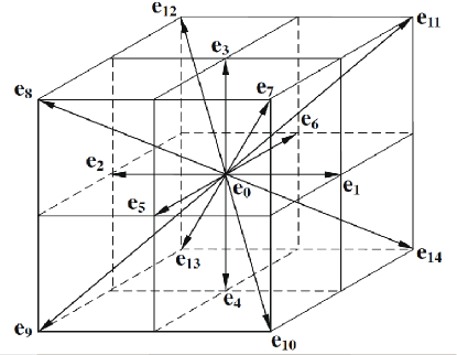
Figure 1: Schematic diagram of the D3Q15 model[28].

We consider the simulation of the incompressible Newtonian fluids where the LBM-D3Q15 model [2] is adopted, and the spatial distribution of the velocities is shown in Figure 1. Following the same notation used by Wu and Shu[28], those 15 lattice velocities are given by

$$e_{\alpha}=\left\{\begin{array}[]{ll}(0,0,0)c&\alpha=0\\ (\pm 1,0,0)c,(0,\pm 1,0)c,(0,0,\pm 1)c&\alpha=1-6\\ (\pm 1,\pm 1,\pm 1)c&\alpha=7-14\end{array}\right.$$ (4)

where $c$ is termed by the lattice speed. The formulation of the lattice Bhatnagar-Gross-Krook model is

$$f_{\alpha}(r+e_{\alpha}\delta_{t},t+\delta_{t})=f_{\alpha}(r,t)-\frac{f_{\alpha}(r,t)-f_{\alpha}^{eq}(r,t)}{\tau}+F_{b}\delta_{t}$$ (5)

where $f_{\alpha}(r,t)$ represents the fluid density distribution function, $r=(x,y,z)$ stands for the space position vector, $t$ denotes time and $\tau$ denotes the non-dimensional relaxation time, $F_{b}\delta_{t}$ denotes the fluid-solid interaction force term which is given in the following section. The equilibrium density distribution function, $f_{\alpha}^{eq}(r,t)$, can be written as

$$f_{\alpha}^{eq}(r,t)=\rho_{f}\omega_{\alpha}[1+3(e_{\alpha}\cdot u)+\frac{9}{2}(e_{\alpha}\cdot u)^{2}-\frac{3}{2}\mid u\mid^{2}]$$ (6)

where the value of weights are: $\omega_{0}=2/9$, $\omega_{\alpha}=1/9$ for $\alpha=1-6$ and $\omega_{\alpha}=1/72$ for $\alpha=7-14$. $u$ denotes the macro velocity at each lattice node which can be calculated by $u=(\sum\limits_{\alpha=0}^{14}f_{\alpha}e_{\alpha})/\rho_{f}$, and the macro fluid density is obtained by $\rho_{f}=\sum\limits_{\alpha=0}^{14}f_{\alpha}$.

2.2 Particulate immersed boundary method (PIBM)

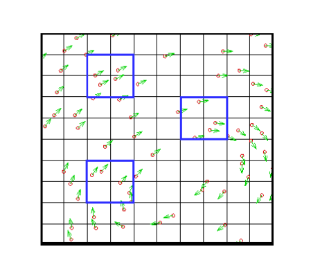
Figure 2: Schematic diagram of the PIBM.

For the sake of clarity, the two-dimensional schematic diagram of the PIBM is given in Figure 2 followed by three-dimensional equation systems. As shown, the fluid is described using the Eulerian square lattices and the solid particles are denoted by the Lagrangian points moving in the flow field. Instead of using several Lagrangian points to construct one large solid particle [1], each Lagrangian point is treated as one single solid particle in this study. The fluid density distribution functions on the solid particles are evaluated using the numerical extrapolation from the circumambient fluid points,

$$f_{\alpha}(X_{l},t)=L\cdot f_{\alpha}(r,t)$$ (7)

where $X_{l}(X,Y,Z)$ is the coordinates of the solid particles, $L$ is the three-dimensional Lagrangian interpolated polynomials,

$$L=\sum\limits_{ijk}\left(\prod\limits_{l=1,l!=i}^{i_{max}}\frac{X-x_{ljk}}{x_{ijk}-x_{ljk}}\right)\left(\prod\limits_{m=1,m!=j}^{j_{max}}\frac{Y-y_{imk}}{y_{ijk}-y_{imk}}\right)\left(\prod\limits_{n=1,n!=k}^{k_{max}}\frac{Z-z_{ijn}}{z_{ijk}-z_{ijn}}\right)$$ (8)

where $i_{max}$, $j_{max}$ and $k_{max}$ are the maximum numbers of the Eulerian points used in the extrapolation as shown by blocks in Figure 2. With the movement of the solid particle, $f_{\alpha}(X_{l},t)$ will be further affected by the particle velocity, $U_{p}$,

$$f_{\beta}(X_{l},t+\delta_{t})=f_{\alpha}(X_{l},t)-2\omega_{\alpha}\rho_{f}\frac{e_{\alpha}U_{p}}{c_{s}^{2}}$$ (9)

where the subscript $\beta$ represents the opposite direction of $\alpha$. Based on the momentum exchange between fluid and particles, the force density, $g(X_{l},t)$, at each solid particle can be calculated using $f_{\alpha}$ and $f_{\beta}$,

$$g(X_{l},t)=\sum\limits_{\beta}e_{\beta}[f_{\beta}(X_{l},t)-f_{\alpha}(X_{l},t)]$$ (10)

The effect on the flow fields from the solid boundary is the body force term $F_{b}\delta_{t}$ in Equation 5, where $F_{b}$ can be expressed by

$$F_{b}=\left(1-\frac{1}{2\tau}\right)\omega_{\alpha}\left(3\frac{e_{\alpha}-u}{c^{2}}+9\frac{e_{\alpha}\cdot u}{c^{4}}e_{\alpha}\right)F(r,t)$$ (11)

and

$$F(r,t)=\sum\limits_{l}g(X_{l},t)D_{ijk}(r_{ijk}-X_{l})A_{p}$$ (12)

$A_{p}$ is the cross-sectional area of the particle which is given as $A_{p}=0.25\pi d_{p}^{2}$, $d_{p}$ is the diameter of the particle. $D_{ijk}$ is used to restrict the feedback force to only take effect on the neighbor of interface and is given by

$$D_{ijk}(r_{ijk}-X_{l})=\frac{1}{h^{3}}\delta_{h}\left(\frac{x_{ijk}-X_{l}}{h}\right)\delta_{h}\left(\frac{y_{ijk}-Y_{l}}{h}\right)\delta_{h}\left(\frac{z_{ijk}-Z_{l}}{h}\right)$$ (13)

with

$$\delta_{h}(a)=\left\{\begin{array}[]{cc}\frac{1}{4}(1+cos(\frac{\pi a}{2})),&when\mid a\mid\leq 2\\ 0,&otherwise\\ \end{array}\right.$$ (14)

where $h$ is the mesh spacing. It should be stressed that by adding a body force on the flow field, the macro moment flux also has to be modified by the force $\rho_{f}u=\sum\limits_{\alpha=0}^{14}f_{\alpha}e_{\alpha}+\frac{1}{2}F(r,t)\delta t$.

On the other hand, the fluid-solid interaction force exerted on the solid particle can be obtained as the reaction force of $g(X_{l},t)$,

$$F_{fpi}=-g(X_{l},t)A_{p}$$ (15)

2.3 Modeling of the particle-particle interactions

The dynamic equations of the particle can be expressed as

$$m\frac{d^{2}r}{dt^{2}} = (1-\frac{\rho_{f}}{\rho_{p}})g+F_{fpi}$$ (16)

$$I\frac{d^{2}\theta}{dt^{2}} = \tau$$ (17)

where $m$ and $I$ are the mass and the moment of inertia of the particle, respectively. $r$ is the particle position and $\theta$ is the angular position. $\rho_{f}$ and $\rho_{p}$ are the densities of the fluid and particle, respectively. $g$ is the gravitational acceleration and $\tau$ is the torque. Considered forces on the right hand side of Equation 16 are the buoyant force and the fluid-particle interaction force $F_{fpi}$. When the particles collide directly with other particles or the walls, the DEM [4] is employed to calculate the collision force. In this study, the particles and walls are directly specified by material properties in the simulation such as density, Young’s modulus and friction coefficient. When the collisions take place, the theory of Hertz [29] is used for modeling the force-displacement relationship while the theory of Mindlin and Deresiewicz [30] is employed for the tangential force-displacement calculations. For two particles of radius $R_{i}$ , Young’s modulus $E_{i}$ and Poisson’s ratios $\nu_{i}$ $(i=1,2)$, the normal force-displacement relationship reads

$$F_{n}=\frac{4}{3}E^{*}R^{*1/2}\delta_{n}^{3/2}$$ (18)

where the equivalent Young’s modulus and radius can be calculated by $1/E^{*}=(1-\nu_{1}^{2})/E_{1}+(1-\nu_{2}^{2})/E_{2}$ and $1/R^{*}=1/R_{1}+1/R_{2}$, respectively.

The incremental tangential force arising from an incremental tangential displacement depends on the loading history as well as the normal force and is given by

$$\Delta T=8G^{*}r_{a}\theta_{k}\Delta\delta_{t}+(-1)^{k}\mu\Delta F_{n}(1-\theta_{k})$$ (19)

where $1/G^{*}=(1-\nu_{1}^{2})/G_{1}+(1-\nu_{2}^{2})/G_{2}$, $r_{a}=\sqrt{\delta_{n}R^{*}}$ is radius of the contact area. $\Delta\delta_{t}$ is the relative tangential incremental surface displacement, $\mu$ is the coefficient of friction, the value of $k$ and $\theta_{k}$ changes with the loading history.

3 Results and discussions

Solid phase		Fluid phase
Density ($kg\cdot m^{-3}$)	1010	Density ($kg\cdot m^{-3}$)	1000
Young’s Module ($GPa$)	68.95	Viscosity ($kg\cdot m^{-1}\cdot s^{-1}$)	1.0e-3
Poisson ratio ($N\cdot m^{-1}$)	0.33	Lattice length ($m$)	0.0001
Friction coefficient ($-$)	0.33	Gravity acceleration ($m\cdot s^{-2}$)	9.8

Table 1: Properties of the particles and fluid.

As stated in previous section, comparing with the conventional IBM, several essential simplifications have been made in the PIBM including removing the constraints between the Lagrangian particles and omitting the calculation of hydrodynamics torque. A natural question is that can the PIBM still success in the complex fluid-particle interaction problems with frequent momentum transfer? For the sake of demonstrating the capability of the PIBM, two- and three-dimensional simulations of particle sedimentation in Newtonian liquid in a cavity were carried out. This configuration is interesting because the Rayleigh-Taylor instability phenomenon may take place on the interface of the agglomerating particles and the fluid. In two-dimensional case [1], the fluid in the lower half of the cavity is found to insert into the upper half and this forms a fluid pocket of mushroom shape in the particle phase interior. Then, the relative smooth interface between the two phase is disturbed and the fluid pocket is teared to small ones. These fluid pockets have the appearance of irregular shape and travel at both vertical and horizontal speed until all the particles fall down on the cavity bottom. In this study, the two-dimensional results by PIBM were directly given due to the fact that the collision rule of the D2Q9 model is very similar to D3Q15 [2] and the two-dimensional code has been tested in  [1]. In the rest of this section, the accuracy of the PIBM was firstly examined by simulating the falling process of a single particle in Newtonian flow and the results were compared with the analytical solutions based on the Stokes’ law. By means of the comparison, the parameters were also calibrated and adopted in the following multi-particle simulations. Then, the two- and three-dimensional results were presented in Section 3.2 and  3.3, respectively. The physical properties of the particles and the surrounding fluid are given in Table 1. It should be mentioned that the lattice spacing length, $h$, is $0.0001m$ in all the simulations.

3.1 Falling of a single particle

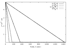
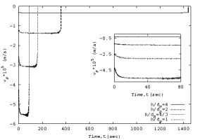
(a)                                               (b)

Figure 3: (a) longitudinal coordinates and (b) longitudinal velocities of the particle under different $h/d_{p}$.

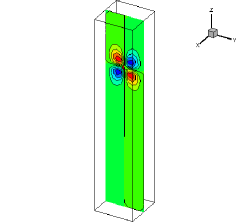
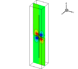
(a)                                               (b)
                 
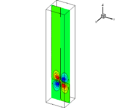
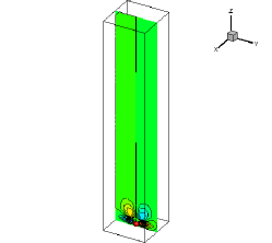
(c)                                               (d)

Figure 4: Instantaneous height of the $0.0001m$ particle with contour plots for $v$ at time (a) $t=22.5s$, (b) $t=45.0s$, (c) $t=67.5s$, (d) $t=90.0s$.

Falling of the single particle in a cuboid cavity was firstly investigated. The length and width of the cuboid cavity are $0.001m$ and the height is $0.005m$. The initial position of the particle is at $(0.0005m,0.0005m,0.0049m)$. Four kinds of particles with different diameters are considered, namely $d_{p}=0.25\times 10^{-4}m$, $0.5\times 10^{-4}m$, $0.75\times 10^{-4}m$ and $10^{-4}m$ or $h/d_{p}=4$, $2$, $4/3$ and $1$, respectively. The largest diameter is equal to one LBM grid spacing length. The longitudinal coordinates and velocities of different particles during the falling process are shown in Figure 3. The particles at rest begin to deposit under the effect of the gravitational force. After a period of acceleration, the particles fall with a constant settling velocity until they approaches to the bottom. The magnitude of the settling velocity increases with the particle size. Finally, the particles stay at the bottom of the cavity with zero longitudinal velocity. Figure 4 shows several typical snapshots of the falling process of the $1\times 10^{-4}m$ particle with contour plots for $v_{f}$, clear influence of the particle motion on the flow structure can be observed. For dilute suspensions, the settling velocity of a single particle in a viscous fluid flow can be evaluated by the Stokes’ law which is given by

$$V_{s}=\dfrac{(\rho_{p}-\rho_{f})d_{p}^{2}g}{18\mu}$$ (20)

where $\mu$ is the dynamic viscosity of the fluid. Quantitative comparison between the results based on the Stokes’ law and the numerical ones are presented in Table 2. As shown, the settling velocities predicted by numerical simulation agree well with the Stokes’ law. However, it is found that the particle may oscillate around the center line during the falling process and the fluctuation on the velocity increases with the particle size especially closing to the cavity bottom. Feng et al. [31] also reported this unsteadiness phenomenon using coupled Direct Numerical Simulation and DEM (DNS-DEM). In the following subsections of this study, $h/d_{p}=4$ and $2$ were chosen based on the similar criterion as adopted in the NS-DEM simulations [32]. Our numerical simulations show that this ratio works well in the multi-particle cases in general, however, further numerical and experimental validations may be needed to fully assess its effect on the particle behaviors.

$h/d_{p}$	Based on Stokes’ law	Numerical results	$\tau$	Physical timestep
	($m/s$)	($m/s$)		($s$)
$4$	$-3.40\times 10^{-6}$	$-3.41\times 10^{-6}$	$0.65$	0.0005
$2$	$-1.36\times 10^{-5}$	$-1.37\times 10^{-5}$	$0.72$	0.0007
$4/3$	$-3.06\times 10^{-5}$	$-3.07\times 10^{-5}$	$0.79$	0.0010
$1$	$-5.44\times 10^{-5}$	$-5.52\times 10^{-5}$	$0.85$	0.0012

Table 2: The settling velocities at different particle size.

3.2 Sedimentation of two-dimensional particles in Newtonian flows

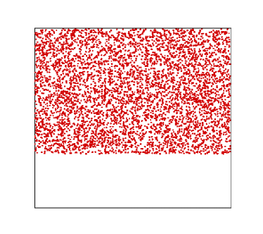
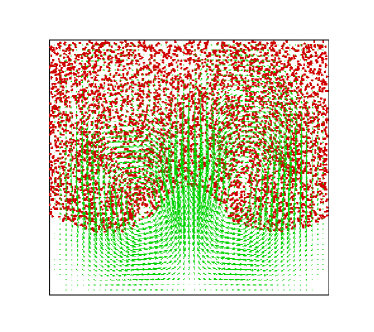
(a)                                               (b)
  
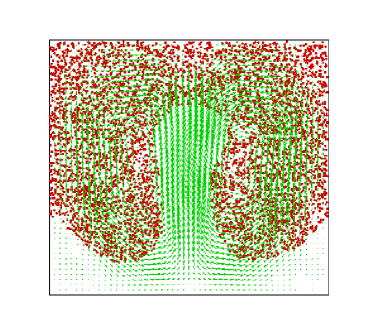
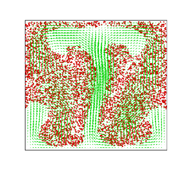
(c)                                               (d)

Figure 5: Instantaneous particle distribution with the fluid velocities at time (a) $t=0.0s$, (b) $t=2.5s$, (c) $t=5.0s$, (d) $t=10.0s$.

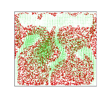
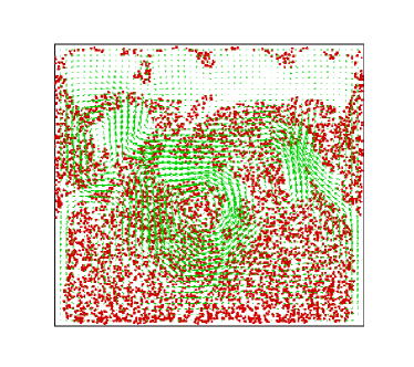
(a)                                               (b)
  
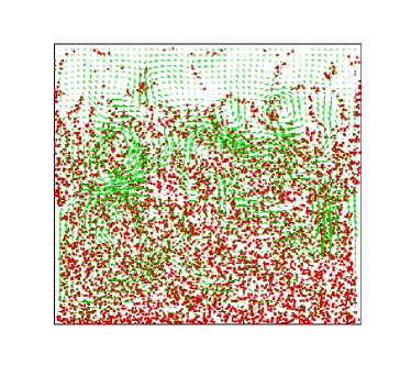
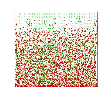
(c)                                               (d)

Figure 6: Instantaneous particle distribution with the fluid velocities at time (a) $t=20.0s$, (b) $t=25.0s$, (c) $t=50.0s$, (d) $t=100.0s$.

Two-dimensional simulations of the particle sedimentation in a square cavity have been conducted using various numerical methods [33, 18, 19, 1]. Here we consider a $0.01m\times 0.01m$ cavity with 5000 two-dimensional particles. The properties of the particles and the surrounding fluid are given in Table 1. The diameter of the particles are $0.25\times 10^{-4}m$ or $h/d_{p}=4$. The relaxation time is $\tau=0.65$, it leads to a physical timestep of $0.0005s$. Initially, the 5000 particles are randomly generated in the upper three-fifths domain and then deposit under the effect of the gravitational force. Figure 5 displays the changing process of the interface line from straight to curve. As expected, the fluid at the lower half of the cavity is swallowed into the the agglomerating particles forming a open hole of mushroom shape. The open hole is shattered to pieces when the particles fall down as shown in Figure 6. Generally speaking, the patterns observed in this simulation are very close to the results provided in the former references [33, 18, 19, 1]. However, compared with the results of large particles that calculated using conventional momentum exchange-based immersed boundary method [1], the whole sedimentation process takes much longer time due to the low settling velocity.

3.3 Sedimentation of three-dimensional particles in Newtonian flows

3.3.1 The sedimentation process

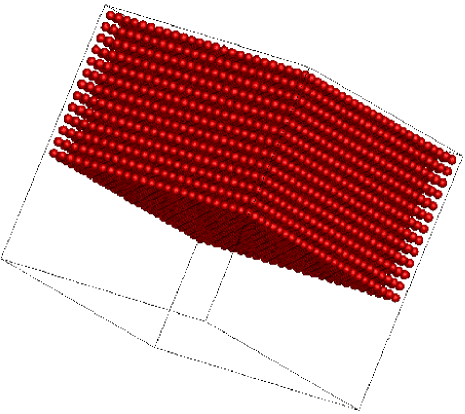
Figure 7: Positions of the 8125 particles at time $t=0.0s$.

In this subsection, a three-dimensional $0.0015m\times 0.00015m\times 0.0015m$ cubic cavity is considered. The diameter of the particles is $0.5\times 10^{-4}m$ or $h/d_{p}=2$. The relaxation time is $\tau=0.72$ which leads to a physical timestep of $0.0007s$. Initially, $8125$ particles are positioned in the upper three-fifths domain as shown in Figure 7, the solid fraction is $0.15$, total volume occupied by the particle assembly is $1.9\times 10^{-9}m^{3}$, total volume of the particles is $5.3\times 10^{-10}m^{3}$ and thus the local porosity is $0.719$. There are vertically 13 layers of particles, in each layer there are $625$ particles forming a $25\times 25$ matrix. In each direction, the particles are uniformly distributed. The gap between the horizontal neighboring particles and between the closest particles and the side wall is about $0.00001m$. The gap between the vertical neighboring particles and between the highest particles and the top wall is about $0.000018m$. The no-slip boundary is adopted on the six boundaries of the cavity, namely the fluid nearby the wall will have zero velocity.

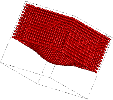
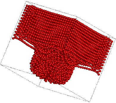
(a)                                               (b)
  
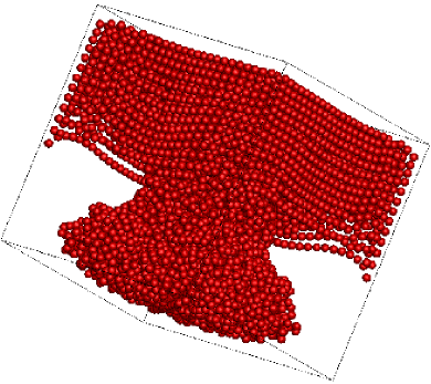
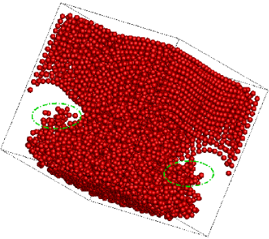
(c)                                               (d)

Figure 8: Positions of the 8125 particles at time (a) $t=2.5s$, (b) $t=5.0s$, (c) $t=7.5s$, (d) $t=10.0s$.

In the initial stages of sedimentation, an overall falling of the particle agglomeration can be observed as shown in Figure 8 (a) and (b). Due to the fact that the initial porosity is low, the whole body at this stage can be regarded as a plug flow creeping in a channel. The distance between the highest particles and the top wall increases gradually and the particle distribution close to the walls does not change significantly. However, instead of settling uniformly, the difference of particle velocity inside and at the bottom of the body shows up shortly. This is because the particles close to the side walls are hindered by the stagnated fluid. Consequently, the particles in the center region move faster and pour down to suck the fluid to fill up the forming gap. The hump grows fast until it reaches the cavity bottom. It can be seen that the changing histories of the fluid-particle interface are different in two- and three-dimensional simulations. In the two-dimensional case, the updraft of the fluid takes place mainly in the center. However, the three-dimensional particle-constructed pestle is too strong to break as shown in Figure 8 (b) and the fluid is pushed away to take a devious route (explained later in Figure 10). This observation is in line with the three-dimensional results reported by Robinson et al. [34] using Smoothed Particle Hydrodynamics (SPH)-DEM simulation. The discrepancy between two- and three-dimensional results is obviously due to the drawback of the two-dimensional assumption.

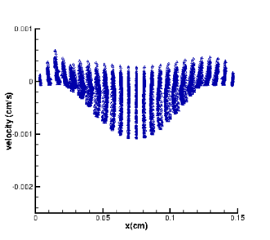
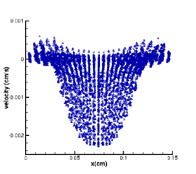
(a)                                               (b)
  
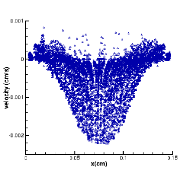
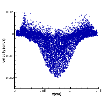
(c)                                               (d)

Figure 9: Particle deposition velocity along the $x-$direction at time (a) $t=2.5s$, (b) $t=5.0s$, (c) $t=7.5s$, (d) $t=10.0s$.

The following three-dimensional deposition processes show nearly opposite trend comparing with the two-dimensional case as shown in Figure 8 (c) and (d). In the two-dimensional case, a fluid hole is formed in the lower half of the cavity which is hugged by two particle arms, this typical phenomenon has been reported in several studies [33, 18, 19, 1]. However, in the three-dimensional case, it is more like a fluid hoop surrounding the particle pestle. The head of the pestle spreads out when it impacts on the bottom. The behavior is not difficult to understand because the successive falling particles keep moving downward and thus pushing on the head. At this time, the underriding of the particles becomes the dominating force in the system and most of the particles distribute in this center region.

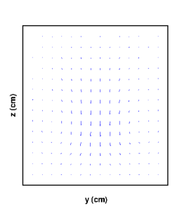
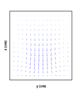
(a)                                               (b)
  
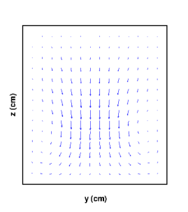
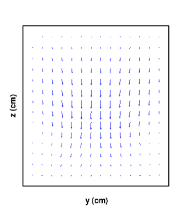
(c)                                               (d)

Figure 10: Instantaneous fluid velocity distribution on the mid-length slice at time (a) $t=2.5s$, (b) $t=5.0s$, (c) $t=7.5s$, (d) $t=10.0s$.

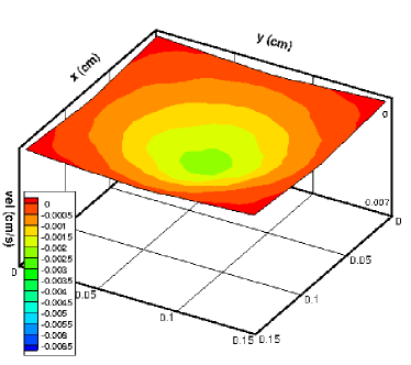
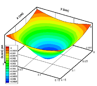
(a)                                               (b)
  
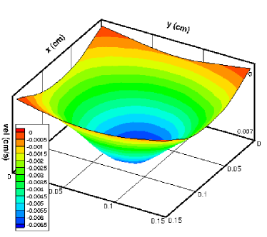
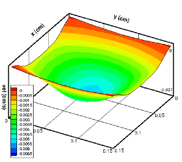
(c)                                               (d)

Figure 11: Overall distribution of the particle deposition velocity at time (a) $t=2.5s$, (b) $t=5.0s$, (c) $t=7.5s$, (d) $t=10.0s$.

Since the particle deposition velocities are very important for the efficiency of the final deposition and may lead to a non-uniform distribution on the bottom. Figure 9 displays the distributions of particle velocity along the $x-$direction before $10.0s$ where large discrepancy can be observed. It is shown that most of the velocities have negative signs and the larger deposition velocities concentrate in the center region. This finding is in line with the particle distribution patterns. Moreover, the magnitude of the deposition velocity increases with time until the particles impact on the bottom. It is also clearly seen that the majority of the velocities in the regions close to the side walls are positive due to the fact that the sucked fluid pushes the high particles up when the center particles sink down. This interesting FSI phenomenon can be clearly observed in Figure 10 where the instantaneous fluid velocity corresponding to Figure 9 is given. It is shown that the initial stagnant fluid is disturbed by the particle motion and follows the trend of the solid particles. Two vortexes (hoop in three-dimensional geometry) are formed in the lower corners of the cavity and the fluid velocity near the side wall is upward. The vortexes are strong when the particle deposition velocities are large. As shown in Figure 9 (c) and (d), the particle deposition velocities begin to decrease after the particles reach the bottom, meanwhile the number of particles with positive velocities increases. These particles are risen by the vortexes and against the falling particles as shown in Figure 8 (d) highlighted by green ellipse. An overall distribution of the particle deposition velocities is given in Figure 11 in terms of mean values. Here, the whole bottom domain is divided by $30\times 30$ squares and then the particles are mapped into the square that the particle center lies. The square holds the deposition velocity that mapped in it. If more than one particle is mapped into the same square, the arithmetic mean value will be employed. As shown, the mean velocities present a generally symmetrical distribution. The particles near the corners deposit significantly slower than the center as results of the fluid viscosity. The highly symmetrical distribution is broken when the particle contact with the bottom. However, a constant symmetrical distribution may not be expected due to the stochastic nature of the solid particles. From $t=10.0s$, the collisions between the particles and particles/walls become the dominating force in the lower half of the cavity. The pestle slumps like an inverted cone and fills the cavity bottom.

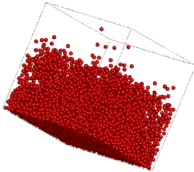
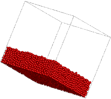
(a)                                               (b)

Figure 12: (a) Positions of the 8125 particles at time $t=50.0s$ and (b) the final distribution.

Figure 12 (a) and (b) display the later stages of the depositing process. In Figure 12 (a), the initially orderly arranged particles are totally disorganized and settle on the cavity bottom length by length.

3.3.2 Effect of the initial porosity

Particle number	Initial porosity	Solid fraction	Initial distribution
$8125$	$0.719$	$0.15$	$25\times 25\times 13$
$5200$	$0.813$	$0.10$	$20\times 20\times 13$
$2925$	$0.888$	$0.056$	$15\times 15\times 13$

Table 3: The settling velocities at different particle size.

It has been well known that the porosity can play an important role in the sedimentation of multi particles. Here, different numbers of particles were positioned in the same region as previous subsection. In other words, the particles would deposit with different initial porosity. The physical properties of the fluid and particles can be found in Table 2. The minimum particle height was monitored to characterize the sedimentation efficiency. The parameters relevant to these simulations are listed in Table. 3.

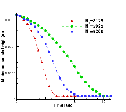
Figure 13: Minimum particle height versus time at different initial porosity.

Figure 13 shows the minimum particle height versus time with different initial porosity. It can be seen that the sedimentation efficiency increases with the decrease of the initial porosity even identical particles were used, this finding is consistent with the analytical results from Robinson et al. [34]. Moreover, a significant deceleration of settling velocity can be observed when the lowest particles approach to the cavity bottom, this phenomenon has also been reported in  [19] and  [1] .

3.3.3 Effect of the particle number on the total computational cost

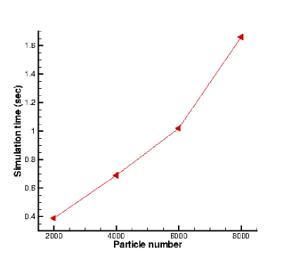
Figure 14: Particle number versus the computational time in one time step.

At last, for the sake of examining the effect of the particle number (the number of the Lagrangian point in conventional IBM) on the total computational cost, several simulations were carried out with different particle number. As shown in Figure 14, the total computational cost increases almost linearly with the particle number and the slope is even larger when the particle number increases from 6000 to 8000. It is worthwhile mentioning that Figure 14 was obtained when there are no particle collisions in the system. We also tested the computing time of each part of the solver in above 8125 particle simulation at time $t=30.0s$, we found that the calculation of the fluid-particle interaction force spends about $84.4\%$ of total simulation time in one time step and the total particle collision number is 6610. Therefore, we come to a conclusion that the total computational cost can be significantly reduced by decreasing the number of the Lagrangian point. Comparing with the conventional LBM-IBM-DEM [1], dozens of times (divided by $N_{LP}$) speedup can be expected in two-dimensional simulation and hundreds of times in three-dimensional simulation under the same particle and mesh number. However, it is worthwhile mentioning that this conclusion is reached only from a computational efficiency point of view. For a certain problem with large range of sizes of particles, a hybrid IBM-PIBM may be needed to achieve high performance calculation which will be discussed in next subsection.

Overall, the main findings of the two- and three-dimensional simulations are summarized as follows: The patterns observed in the two-dimensional simulation are close to the results provided in former references [33, 18, 19, 1]. However, the three-dimensional results show large discrepancy with the two-dimensional results which is most probably due to the two-dimensional assumption. Imaging a case in a enclosed container like a fluidization bed, the fluid is unpenetrable into a two-dimensional well-packed particle bed without breaking the compact structure, whereas penetration into a three-dimensional bed is somehow possible because the geometry is much more polyporous and complex.

3.3.4 Hybrid IBM-PIBM modeling

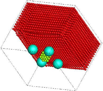
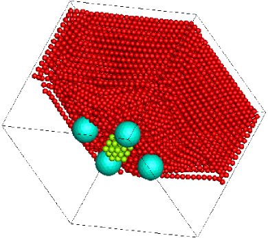
(a)                                               (b)
  
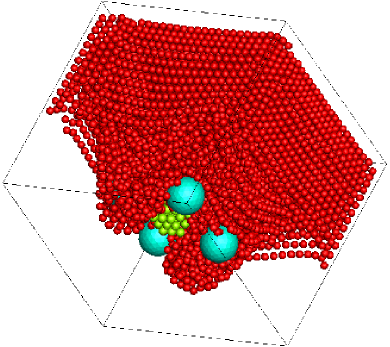
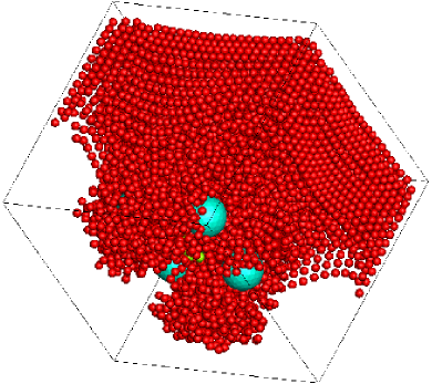
(c)                                               (d)

Figure 15: Positions of the 8125 particles with obstacles at time (a) $t=2.5.0s$, (b) $t=5.0s$, (c) $t=7.5s$, (d) $t=10.0s$.

It is common to encounter a system containing various sizes of particles. A multiscale analysis is preferred when the size range is large. If all the particles are treated using the conventional IBM, the number of grids required to construct the finest particle would make the whole simulation too expensive. On the contrary, if all the coupling work is carried out based on the PIBM, the grid required to embody the largest particle would be too coarse to accurately reflect the fluid flow. A more frequently encountered requirement is to build the complex boundaries or irregular elements using IBM. In other words, a hybrid IBM-PIBM method is needed. Using a simply sample as shown in Figure 12, the advantage of this mixed approach can be seen where five stationary obstacles are fixed below the particles (four large particles and one cube consisting of 27 small particles). The four large particles are established using the conventional IBM while the rest, including the 27 particle for the cube, are treated using PIBM. The criterion to choose different methods is the ratio between the particle size and the lattice spacing. In general, the grid size can be specified at 10 times the particle sizes in the Eulerian-Eulerian model [35] and about 5 times in the Eulerian-Lagrangian model based on NS-DEM [32]. However, the results from current study indicate that the ratio can be 2 in LBM-PIBM-DEM though the optimal ratio is still in question.

4 Concluding remarks

A PIBM for simulating the particulate flow in fluid was presented. Compared with the conventional momentum exchange-based IBM, no artificial parameters are introduced and the implementation is simpler. The PIBM is more suitable for simulating the motion of a large number of particles in fluid, particularly in the three-dimensional cases where particle collisions dominate. Dozens of times speedup can be expected in two-dimensional simulation and hundreds of times in three-dimensional simulation under the same particle and mesh number.

Numerical simulations were carried out based on the LBM-PIBM-DEM scheme, our result of falling of single particle reveals that the settling velocity predicted by numerical simulation agrees well with the Stokes’ law. Further multi-particle simulation results confirm that the LBM-PIBM-DEM scheme can capture the feature of the particulate flows in fluid and is a promising strategy for the solution of the particle-fluid interaction problems. By comparing two- and three-dimensional results, essential discrepancy was found due to the drawback of the two-dimensional assumption. Therefore, it can be concluded that the two-dimensional simulations may be good as a first and cheaper approach, the three-dimensional simulations are necessary for an accurate description of the particle behaviors as well as the flow patterns. From our three-dimensional results by PIBM, the sedimentation efficiency of particle is found to increase with the decrease of initial porosity.

Due to the fact that the calculation of the fluid-particle interaction force in the PIBM is simply based on the momentum conservation of the fluid particle, the LBM-PIBM-DEM scheme can be easily connected with other CFD solvers or Lagrangian particle tracking method where the conventional IBM works, e.g. with the direct numerical simulation [31]. However, during the simulations, we found that numerical instability may occur when the particle velocity is high, which seems to be a general weakness of the IBM family methods. For the sake of achieving validate results, the PIBM users are recommended to conduct a simplified case to compare with the analytical solutions/experimental observation to tune the LBM relaxation time, $\tau$, before using it in the multi-particle simulations. This practice is competent and has been widely used in LBM-DEM [19, 36] and other simulations based on DEM [37, 38].

References

References

- [1] H. Zhang, Y. Tan, S. Shu, X. Niu, F. X. Trias, D. Yang, H. Li, Y. Sheng, Numerical investigation on the role of discrete element method in combined LBM-IBM-DEM modeling, Computers & Fluids 94 (2014) 37 – 48.
- [2] Qian, YH and d’Humières, Dominique and Lallemand, Pierre, Lattice BGK models for Navier-Stokes equation, EPL (Europhysics Letters) 17 (6) (1992) 479.
- [3] C. S. Peskin, Numerical analysis of blood flow in the heart, Journal of Computational Physics 25 (3) (1977) 220 – 252.
- [4] P. Cundall, A computer model for simulating progressive large scale movements in blocky system, In: Muller led, ed. Proc Symp Int Soc Rock Mechanics, Rotterdam: Balkama A A 1 (1971) 8–12.
- [5] X. Yue, H. Zhang, C. Luo, S. Shu, C. Feng, Parallelization of a DEM Code Based on CPU-GPU Heterogeneous Architecture, Parallel Computational Fluid Dynamics (2014) 149–159.
- [6] K. Kafui, S. Johnson, C. Thornton, J. Seville, Parallelization of a Lagrangian-Eulerian DEM/CFD code for application to fluidized beds, Powder Technology 207 (2011) 270–278.
- [7] H. Zhang, F. X. Trias, Y. Tan, Y.Sheng, A. Oliva, Parallelization of a DEM/CFD code for the numerical simulation of particle-laden turbulent flow, 23rd International Conference on Parallel Computational Fluid Dynamics, Barcelona (2011) 1–5.
- [8] Y. Tan, H. Zhang, D. Yang, S. Jiang, J. Song, Y. Sheng, Numerical simulation of concrete pumping process and investigation of wear mechanism of the piping wall, Tribology International 46 (1) (2012) 137 – 144.
- [9] H. Zhang, Y. Tan, D. Yang, F. X. Trias, S. Jiang, Y. Sheng, A. Oliva, Numerical investigation of the location of maximum erosive wear damage in elbow: Effect of slurry velocity, bend orientation and angle of elbow, Powder Technology 217 (2012) 467 – 476.
- [10] D. R. Felice, The Voidage Function for Fluid-particle Interaction Systems, International Journal on Multiphase Flow 20 (1994) 153–159.
- [11] B. Cook, D. Noble, J. Williams, A direct simulation method for particle-fluid systems, Engineering Computation 21 (2004) 151–168.
- [12] K. Han, Y. Feng, D. Owen, Coupled lattice Boltzmann and discrete element modelling of fluid–particle interaction problems, Computers and Structures 85 (11-14) (2007) 1080 – 1088.
- [13] H. Zhang, Y. Tan, M. Li, A Numerical Simulation of Motion of Particles under the Wafer in CMP, International Conference on Computer Science and Software Engineering 3 (2008) 31–34.
- [14] X. Cui, J. Li, A. Chan, D. Chapman, Coupled DEM-LBM simulation of internal fluidisation induced by a leaking pipe, Powder Technology 254 (2014) 299 – 306.
- [15] H. Zhu, Z. Zhou, R. Yang, A. Yu, Discrete particle simulation of particulate systems: theoretical developments, Chemical Engineering Science 62 (13) (2007) 3378–3396.
- [16] A. B. Yu, B. H. Xu, Particle-scale modelling of gas–solid flow in fluidisation, Journal of Chemical Technology and Biotechnology 78 (2-3) (2003) 111–121.
- [17] D. R. Noble, J. R. Torczynski, A Lattice-Boltzmann Method for Partially Saturated Computational Cells, International Journal of Modern Physics C 09 (08) (1998) 1189–1201.
- [18] Z.-G. Feng, E. E. Michaelides, The immersed boundary-lattice Boltzmann method for solving fluid–particles interaction problems, Journal of Computational Physics 195 (2) (2004) 602 – 628.
- [19] Z.-G. Feng, E. E. Michaelides, Proteus: a direct forcing method in the simulations of particulate flows, Journal of Computational Physics 202 (1) (2005) 20 – 51.
- [20] X. Niu, C. Shu, Y. Chew, Y. Peng, A momentum exchange-based immersed boundary-lattice Boltzmann method for simulating incompressible viscous flows, Physics Letters A 354 (3) (2006) 173 – 182.
- [21] J. Wu, C. Shu, Y. H. Zhang, Simulation of incompressible viscous flows around moving objects by a variant of immersed boundary-lattice Boltzmann method, International Journal for Numerical Methods in Fluids 62 (3) (2010) 327–354.
- [22] H.-Z. Yuan, X.-D. Niu, S. Shu, M. Li, H. Yamaguchi, A momentum exchange-based immersed boundary-lattice Boltzmann method for simulating a flexible filament in an incompressible flow, Computers & Mathematics with Applications 67 (5) (2014) 1039 – 1056.
- [23] Y. Wang, C. Shu, C. Teo, Thermal lattice Boltzmann flux solver and its application for simulation of incompressible thermal flows, Computers & Fluids 94 (2014) 98 – 111.
- [24] Y. Hu, X.-D. Niu, S. Shu, H. Yuan, M. Li, Natural Convection in a Concentric Annulus: A Lattice Boltzmann Method Study with Boundary Condition-Enforced Immersed Boundary Method, Advances in Applied Mathematics and Mechanics 5 (2013) 321–336.
- [25] J. Wu, C. Shu, Particulate Flow Simulation via a Boundary Condition-Enforced Immersed Boundary-Lattice Boltzmann Scheme, Communications in Computational Physics 7 (2010) 793–812.
- [26] L. Wang, B. Zhang, X. Wang, W. Ge, J. Li, Lattice Boltzmann based discrete simulation for gas–solid fluidization, Chemical Engineering Science 101 (2013) 228–239.
- [27] J. Li, Particle-fluid two-phase flow: the energy-minimization multi-scale method, Metallurgical Industry Press, 1994.
- [28] J. Wu, C. Shu, An improved immersed boundary-lattice Boltzmann method for simulating three-dimensional incompressible flows, Journal of Computational Physics 229 (13) (2010) 5022 – 5042.
- [29] K. Johnson, Contact mechanics, Cambridge University Press, Cambridge.
- [30] R. Mindlin, H. Deresiewicz, Elastic spheres in contact under varying oblique forces, Journal of Applied Mechanics 20 (1953) 327–344.
- [31] Z.-G. Feng, M. E. C. Ponton, E. E. Michaelides, S. Mao, Using the direct numerical simulation to compute the slip boundary condition of the solid phase in two-fluid model simulations, Powder Technology (0) (2014) –.
- [32] K. Kafui, C. Thornton, M. Adams, Discrete particle-continuum fluid modelling of gas–solid fluidised beds, Chemical Engineering Science 57 (13) (2002) 2395–2410.
- [33] R. Glowinski, T.-W. Pan, T. I. Hesla, D. D. Joseph, A distributed lagrange multiplier/fictitious domain method for particulate flows, International Journal of Multiphase Flow 25 (5) (1999) 755–794.
- [34] M. Robinson, M. Ramaioli, S. Luding, Fluid–particle flow simulations using two-way-coupled mesoscale SPH–DEM and validation, International Journal of Multiphase Flow 59 (0) (2014) 121 – 134.
- [35] S. Cloete, S. Amini, S. T. Johansen, A fine resolution parametric study on the numerical simulation of gas–solid flows in a periodic riser section, Powder Technology 205 (1) (2011) 103–111.
- [36] Z.-G. Feng, E. E. Michaelides, Robust treatment of no-slip boundary condition and velocity updating for the lattice-boltzmann simulation of particulate flows, Computers & Fluids 38 (2) (2009) 370–381.
- [37] Y. Tan, D. Yang, Y. Sheng, Study of polycrystalline Al2O3 machining cracks using discrete element method, International Journal of Machine Tools and Manufacture 48 (9) (2008) 975 – 982.
- [38] Y. Tan, D. Yang, Y. Sheng, Discrete element method (DEM) modeling of fracture and damage in the machining process of polycrystalline SiC, Journal of the European Ceramic Society 29 (6) (2009) 1029 – 1037.