The isospin asymmetry in $B\to K^{*}\mu^{+}\mu^{-}$ using AdS/QCD

Abstract

We compute the isospin asymmetry distribution in the rare dileptonic decay $B\to K^{*}\mu^{+}\mu^{-}$, in the dimuon mass squared ($q^{2}$) region below the $J/\Psi$ resonance, using non-perturbative inputs as predicted by the anti-de Sitter/Quantum Chromodynamics (AdS/QCD) correspondence and by Sum Rules. We predict a positive asymmetry at $q^{2}=0$ which flips sign in the region $q^{2}\in[1,2]~{}\mbox{GeV}^{2}$ to remain small ($\leq 2\%$) and negative for larger $q^{2}$. While our predictions are distinct as $q^{2}\to 0$, they become hardly model-dependent $q^{2}\geq 4~{}\mbox{GeV}^{2}$. We compare our predictions to the most recent LHCb data.

I Introduction

The rare decay $B\to K^{*}\mu^{+}\mu^{-}$ has recently been attracting much attention from both the experimental Aaij et al. (2014); Aaltonen et al. (2012); Lees et al. (2012); Wei et al. (2009); Aaij et al. (2013a, 2012, b); LHC (2012) and theoretical Altmannshofer and Straub (2013); Descotes-Genon et al. (2013a); Hurth and Mahmoudi (2013); Descotes-Genon et al. (2013b); Gauld et al. (2013a); Buras and Girrbach (2013); Gauld et al. (2013b); Hambrock et al. (2013); Khodjamirian et al. (2010); Bharucha et al. (2010); Datta et al. (2013); Alok et al. (2010) sides because various observables associated with this decay are susceptible to reveal New Physics effects. An interesting observable to look at is the isospin asymmetry distribution defined as

$$A_{I}(q^{2})=\frac{\mathrm{d}\Gamma(B^{0}\to K^{*0}\mu^{+}\mu^{-})/\mathrm{d}q^{2}-\mathrm{d}\Gamma(B^{+}\to K^{*+}\mu^{+}\mu^{-})/\mathrm{d}q^{2}}{\mathrm{d}\Gamma(B^{0}\to K^{*0}\mu^{+}\mu^{-})/\mathrm{d}q^{2}+\mathrm{d}\Gamma(B^{+}\to K^{*+}\mu^{+}\mu^{-})/\mathrm{d}q^{2}}$$ (1)

since being a ratio of differential decay widths, the leading uncertainties in the $B\to K^{*}$ form factors cancel in the theoretical computation of this asymmetry. Nevertheless, there remains some model-dependence in theory predictions which we address in this paper.

In a previous paper Ahmady and Sandapen (2013), two of us have computed the isospin asymmetry in $B\to K^{*}\gamma$ where we highlighted that an advantage of using an AdS/QCD twist-$2$ DA is that it avoids the end-point divergence encountered with the corresponding Sum Rules DA. We now extend our calculation for $B\to K^{*}l^{+}l^{-}$, i.e. for the case $q^{2}\neq 0$, where $q^{2}$ is the dimuon mass squared. This isospin aymmetry distribution has recently been measured by the LHCb Collaboration at $3~{}\mbox{fb}^{-1}$ Aaij et al. (2014) superseding the previous LHCb measurements at $1~{}\mbox{fb}^{-1}$ given in Ref.Aaij et al. (2012). The original SM computation of the isospin asymmetry in $B\to K^{*}\mu^{+}\mu^{-}$ was performed by Feldmann and Matias in Ref. Feldmann and Matias (2003) which we follow here. A more sophisticated calculation of this isospin asymmetry has recently been performed by Lyon and Zwicky in Ref. Lyon and Zwicky (2013).

A potential source of theoretical uncertainty in the SM prediction arises from the model-dependent non perturbative quantities, namely the Distribution Amplitudes and decay constants of the $K^{*}$ as well as the two universal soft $B\to K^{*}$ transition form factors. The latter form factors are deduced from the seven $B\to K^{*}$ form factors which themselves can be obtained from lattice QCD at high $q^{2}$ Horgan et al. (2013) and from light-cone sum rules (LCSR) at low to moderate $q^{2}$ Aliev et al. (1997) . LCSR require as non-perturbative inputs the model-dependent DAs of the $K^{*}$ meson as well as its decay constants.

Our goal in this paper is to repeat the computation of Ref. Feldmann and Matias (2003) for the isospin asymmetry distribution in $B\to K^{*}l^{+}l^{-}$ but with different inputs for the non-perturbative quantities mentioned above. We compute the decay constants and the DAs of the $K^{*}$ using AdS/QCD Ahmady and Sandapen (2013) while we build upon our previous work Ahmady et al. (2014) to obtain the two universal $B\to K^{*}$ soft form factors. To investigate the degree of model-dependence, we shall compare our AdS/QCD prediction to that obtained using Sum Rules DAs and decay constants.

II The isospin asymmetry

In the QCD factorization approach, the isospin asymmetry distribution is given by Feldmann and Matias (2003)

$$A_{I}(q^{2})=\Re e(b_{d}^{\perp}(q^{2})-b_{u}^{\perp}(q^{2}))\frac{|\mathcal{C}_{9}^{(0)\perp}(q^{2})|^{2}}{|C_{10}(\mu_{b})|^{2}+|\mathcal{C}_{9}^{(0)\perp}(q^{2})|^{2}}\times\frac{F(q^{2})}{G(q^{2})}$$ (2)

with

$$F(q^{2})=1+\frac{1}{4}\frac{E_{K^{*}}^{2}m_{B}^{2}}{q^{2}m_{K^{*}}^{2}}\frac{\xi_{\parallel}^{2}(q^{2})}{\xi_{\perp}^{2}(q^{2})}\frac{\Re e(b_{d}^{\parallel}(q^{2})-b_{u}^{\parallel}(q^{2}))}{\Re e(b_{d}^{\perp}(q^{2})-b_{u}^{\perp}(q^{2}))}\frac{|\mathcal{C}_{9}^{(0)\parallel}(q^{2})|^{2}}{|\mathcal{C}_{9}^{(0)\perp}(q^{2})|^{2}}$$ (3)

and

$$G(q^{2})=1+\frac{1}{4}\frac{E_{K^{*}}^{2}m_{B}^{2}}{q^{2}m_{K^{*}}^{2}}\frac{\xi_{\parallel}^{2}(q^{2})}{\xi_{\perp}^{2}(q^{2})}\frac{|\mathcal{C}_{9}^{(0)\parallel}(q^{2})|^{2}+|C_{10}(\mu_{b})|^{2}}{|\mathcal{C}_{9}^{(0)\perp}(q^{2})|^{2}+|C_{10}(\mu_{b})|^{2}}$$ (4)

where $E_{K^{*}}=(m_{B}^{2}-q^{2})/(2m_{B})$ is the energy of the $K^{*}$ meson. The generalized SM Wilson coefficients are given by

$$C_{9}^{(0)\perp}(q^{2})=C_{9}(\mu_{b})+Y(q^{2})+\frac{2m_{b}m_{B}}{q^{2}}C_{7}^{\rm eff}(\mu_{b})$$ (5)

and

$$C_{9}^{(0)\parallel}(q^{2})=C_{9}(\mu_{b})+Y(q^{2})+\frac{2m_{b}}{m_{B}}C_{7}^{\rm eff}(\mu_{b})\;.$$ (6)

As noted in Ref. Feldmann and Matias (2003), in the limit $q^{2}\to 0$, the photon pole in $C_{9}^{(0)\perp}$ dominates and Eqn. (2) becomes

$$A_{I}(0)=\Re e(b_{d}^{\perp}(0)-b_{u}^{\perp}(0))$$ (7)

which is the isospin asymmetry in $B\to K^{*}\gamma$ computed originally in Ref. Kagan and Neubert (2002). In the definitions (5) and (6), the function $Y(q^{2})$ is given by Beneke et al. (2001)

$$Y(q^{2}) = h(q^{2},m_{c},\mu_{b})\left(3\overline{C}_{1}(\mu_{b})+\overline{C}_{2}(\mu_{b})+3\overline{C}_{3}(\mu_{b})+\overline{C}_{4}(\mu_{b})+3\overline{C}_{5}(\mu_{b})+\overline{C}_{6}(\mu_{b})\right)$$ (8)

$$- \,\frac{1}{2}\,h(q^{2},m_{b},\mu_{b})\left(4\,(\overline{C}_{3}(\mu_{b})+\overline{C}_{4}(\mu_{b}))+3\overline{C}_{5}(\mu_{b})+\overline{C}_{6}(\mu_{b})\right)$$

$$- \frac{1}{2}\,h(q^{2},0,\mu_{b})\left(\overline{C}_{3}(\mu_{b})+3\overline{C}_{4}(\mu_{b})\right)+\,\frac{2}{9}\,\left(\frac{2}{3}\overline{C}_{3}(\mu_{b})+2\overline{C}_{4}(\mu_{b})+\frac{16}{3}\overline{C}_{5}(\mu_{b})\right)$$

where the vacuum polarisation function

$$h(q^{2},m_{q},\mu_{b})=-\frac{4}{9}\left(6\int_{0}^{1}x(1-x)\ln(m_{q}^{2}-x(1-x)q^{2}-i\epsilon)\mathrm{d}x-\ln(\mu_{b}^{2})+1\right)\;.$$ (9)

In Eqns. (2) and (3),

$$b_{q}^{\perp}(q^{2})=\frac{24\pi^{2}m_{B}f_{B}e_{q}}{q^{2}\xi_{\perp}(q^{2})\mathcal{C}_{9}^{(0)\perp}(q^{2})}\left(\frac{f_{K^{*}}^{\perp}}{m_{b}}K_{1}^{\perp}(q^{2})+\frac{f_{K}^{*}m_{K}^{*}}{6\lambda_{B,+}(q^{2})m_{B}}\frac{K_{2}^{\perp}(q^{2})}{1-q^{2}/m_{B}^{2}}\right)$$ (10)

and

$$b_{q}^{\parallel}(q^{2})=\frac{24\pi^{2}f_{B}e_{q}m_{K^{*}}}{m_{B}E_{K^{*}}\xi_{\parallel}(q^{2})\mathcal{C}_{9}^{(0)\parallel}(q^{2})}\left(\frac{f_{K^{*}}}{3\lambda_{B,-}(q^{2})}K_{1}^{\parallel}(q^{2})\right)$$ (11)

where we take $f_{B}=0.190$ GeV. In Eqn. (10),

$$K_{1}^{\perp}(q^{2})=K_{1}^{\perp(a)}(q^{2})+K_{1}^{\perp(b)}(q^{2})+K_{1}^{\perp(c)}(q^{2})$$ (12)

with

$$K_{1}^{\perp(a)}(q^{2})=-\left(\overline{C}_{6}(\mu_{h})+\frac{\overline{C}_{5}(\mu_{h})}{N_{c}}\right)F_{\perp}(\hat{s}),\hskip 14.22636ptF_{\perp}(\hat{s})=\frac{1}{3}\int_{0}^{1}\mathrm{d}u\frac{\phi_{\perp}(u)}{\bar{u}+u\hat{s}}\;,$$ (13)

$$K_{1}^{\perp(b)}(q^{2})=C_{8}^{\rm eff}(\mu_{h})\frac{m_{b}^{2}}{m_{B}^{2}}\frac{C_{F}}{N_{c}}\frac{\alpha_{s}(\mu_{h})}{4\pi}X_{\perp}(\hat{s}),\hskip 14.22636ptX_{\perp}(\hat{s})=F_{\perp}(\hat{s})+\frac{1}{3}\int_{0}^{1}\mathrm{d}u\frac{\phi_{K^{*}}^{\perp}(u)}{(\bar{u}+u\hat{s})^{2}}\;,$$ (14)

$$K_{1}^{\perp(c)}(q^{2})=\frac{C_{F}}{N_{c}}\frac{\alpha_{s}(\mu_{h})}{4\pi}\frac{2}{3}\int_{0}^{1}\mathrm{d}u\frac{\phi_{K^{*}}^{\perp}(u)}{\bar{u}+u\hat{s}}F_{V}(\bar{u}m_{b}^{2}+uq^{2})\;$$ (15)

and

$$K_{2}^{\perp}(q^{2})=K_{2}^{\perp(a)}(q^{2})+K_{2}^{\perp(b)}(q^{2})+K_{2}^{\perp(c)}(q^{2})$$ (16)

with

$$K_{2}^{\perp(a)}(q^{2})=-\frac{\lambda_{u}}{\lambda_{t}}\left(\frac{\overline{C}_{1}}{3}(\mu_{h})+\overline{C}_{2}(\mu_{h})\right)\delta_{qu}+\left(\overline{C}_{4}(\mu_{h})+\frac{\overline{C}_{3}(\mu_{h})}{3}\right)\;,$$ (17)

$$K_{2}^{\perp(b)}(q^{2})=\mathcal{O}\left(\frac{\Lambda_{h}}{m_{B}}\right)\;,$$ (18)

$$K_{2}^{\perp(c)}(q^{2})=-\frac{C_{F}}{N_{c}}\frac{\alpha_{s}(\mu_{h})}{4\pi}2\int_{0}^{1}\mathrm{d}u\left(g_{\perp}^{(v)}(u)-\frac{{g^{\prime}}_{\perp}^{(a)}(u)}{4}\right)F_{V}(\bar{u}m_{b}^{2}+uq^{2})\;.$$ (19)

In Eqn. (11),

$$K_{1}^{\parallel}(q^{2})=K_{1}^{\parallel(a)}(q^{2})+K_{1}^{\parallel(b)}(q^{2})+K_{1}^{\parallel(c)}(q^{2})$$ (20)

with

$$K_{1}^{\parallel(a)}(q^{2})=K_{2}^{\perp(a)}(q^{2})$$ (21)

$$K_{1}^{\parallel(b)}(q^{2})=-C_{8}^{\rm eff}(\mu_{h})\frac{m_{b}}{m_{B}}\frac{C_{F}}{N_{c}}\frac{\alpha_{s}(\mu_{h})}{4\pi}F_{\parallel}(\hat{s}),\hskip 14.22636ptF_{\parallel}(\hat{s})=2\int_{0}^{1}\mathrm{d}u\frac{\phi_{\parallel}(u)}{\bar{u}+u\hat{s}}\;,$$ (22)

$$K_{1}^{\parallel(c)}(q^{2})=-\frac{C_{F}}{N_{c}}\frac{\alpha_{s}(\mu_{h})}{4\pi}2\int_{0}^{1}\mathrm{d}u\phi_{\parallel}(u)F_{V}(\bar{u}m_{b}^{2}+uq^{2})\;.$$ (23)

The vector form factor $F_{V}(s)$ appearing in Eqns (15), (19), and (23) is given as Feldmann and Matias (2003)

$$F_{V}(s) = \frac{3}{4}\{h(s,m_{c},\mu_{h})\,(\overline{C}_{2}(\mu_{h})+\overline{C}_{4}(\mu_{h})+\overline{C}_{6}(\mu_{h}))$$

$$+ h(s,m_{b},\mu_{h})\,(\overline{C}_{3}(\mu_{h})+\overline{C}_{4}(\mu_{h})+\overline{C}_{6}(\mu_{h}))$$

$$+ h(s,0,\mu_{h})\,(\overline{C}_{3}(\mu_{h})+3\overline{C}_{4}(\mu_{h})+3\overline{C}_{6}(\mu_{h}))-\frac{8}{27}\,(\overline{C}_{3}(\mu_{h})-\overline{C}_{5}(\mu_{h})-15\overline{C}_{6}(\mu_{h}))\}$$

Finally, in Eqns (10) and (11),

$$\lambda_{B,\pm}^{-1}(q^{2})=\int_{0}^{\infty}d\omega\,\frac{\phi^{B}_{\pm}(\omega)}{\omega-q^{2}/m_{B}-i\epsilon}\ .$$ (25)

where $\phi^{B}_{\pm}(\omega)$ are given in Ref. Beneke and Feldmann (2001).

Note that some of the above equations differ from those given in Ref. Feldmann and Matias (2003). First, we take the argument of $F_{V}$ to be $\bar{u}m_{b}^{2}+uq^{2}$ instead of $\bar{u}m_{B}^{2}+uq^{2}$. Secondly, in Eq. (10), we write $(f_{K^{*}}^{\perp}/m_{b})$ instead of $(f_{K^{*}}^{\perp}/m_{B})$. Thirdly, in Eqn. (14), we have $(m_{b}^{2}/m_{B}^{2})$ instead of $(m_{b}/m_{B})$. Finally, we have an additional factor of $4$ on the right-hand-side of Eqn. (19). In this way, we are able to recover the expression for $A_{I}(0)$ as derived in Ref. Kagan and Neubert (2002). The numerical impact of these changes is small.

In the above equations, we have made explicit the scale dependence of the next-to-leading log (NLL) Wilson coeffecients which we take at $\mu_{b}\sim m_{b}$ or at the hadronic scale $\mu_{h}=\sqrt{\Lambda_{h}\mu_{b}}$ ($\Lambda_{h}=0.5~{}\mbox{GeV}$). We take $m_{b}=4.6~{}\mbox{GeV}$ following Ref. Feldmann and Matias (2003). We evolve the Wilson coefficients from the electroweak scale $\mu_{W}=M_{W}$ down to the scales $\mu_{b,h}$ using the renormalization group equations. Details of this computation can be found in Appendix B. The resulting values of the NLL Wilson coefficients at the two scales $\mu=m_{b}$ and $\mu=\sqrt{\Lambda_{h}m_{b}}$ are shown in Table 1. Note that we use the $3$-loop formula for the running strong coupling $\alpha_{s}$ (see Appendix A).

Table 1: NLL Wilson coefficients at the scale $\mu_{b}=4.6\,$GeV and $\mu_{h}=1.52$ GeV. Input parameters are $\alpha_{s}(M_{z})=0.1184$, $m_{t}^{\rm pole}=173.5$ GeV, $M_{W}=80.385$ GeV and $\sin^{2}\!\theta_{W}=0.23$.

	${\overline{C}}_{1}$	${\overline{C}}_{2}$	${\overline{C}}_{3}$	${\overline{C}}_{4}$	${\overline{C}}_{5}$	${\overline{C}}_{6}$
$\mu_{b}$	$-0.1482$	$1.0597$	$0.0116$	$-0.0347$	$0.0099$	$-0.0393$
$\mu_{h}$	$-0.3423$	$1.1577$	$0.0223$	$-0.0629$	$0.0179$	$-0.0912$
	$C_{7}^{\rm eff}$	$C_{8}^{\rm eff}$	$C_{9}$	$C_{10}$
$\mu_{b}$	$-0.3075$	$-0.1690$	$4.2381$	$-4.6405$
$\mu_{h}$	$-0.3590$	$-0.2112$	$4.5019$	$-4.6405$

III Distribution Amplitudes and Soft Form factors

We now focus on the non-perturbative inputs namely the Distribution Amplitudes (and decay constants) as well as the soft form factors. In Eqns. (13), (14) and (15), $\phi_{K^{*}}^{\perp}(u)$ is the twist-$2$ DA of the transversely polarized $K^{*}$ while in Eqns. (22), (23), $\phi_{K^{*}}^{\parallel}(u)$ is the twist-$2$ DA of the longitudinally polarized $K^{*}$. Note that, to leading twist-$2$ accuracy, the DAs $g_{K^{*}}^{\perp(v,a)}(u)$ appearing in Eqn. (19) can be expressed in terms of the twist-$2$ DA $\phi_{\parallel}(u)$ Kagan and Neubert (2002). In this paper, we shall use the AdS/QCD holographic twist-$2$ DAs which were derived previously in Ref. Ahmady and Sandapen (2013):

$$\phi_{K^{*}}^{\parallel}(z,\mu)=\frac{N_{c}}{\pi f_{K^{*}}M_{K^{*}}}\int\mathrm{d}r\mu J_{1}(\mu r)[M_{K^{*}}^{2}z(1-z)+m_{\bar{q}}m_{s}-\nabla_{r}^{2}]\frac{\phi_{K^{*}}^{L}(r,z)}{z(1-z)}\;,$$ (26)

$$\phi_{K^{*}}^{\perp}(z,\mu)=\frac{N_{c}}{\pi f_{K*}^{\perp}}\int\mathrm{d}r\mu J_{1}(\mu r)[m_{s}-z(m_{s}-m_{\bar{q}})]\frac{\phi_{K^{*}}^{T}(r,z)}{z(1-z)}\;,$$ (27)

where $\phi_{K^{*}}^{L,T}(r,z)$ are the holographic wavefunctions obtained by solving the holographic light-front Schroedinger equation de Teramond and Brodsky (2009, 2012); Brodsky et al. (2013). Explicitly Ahmady and Sandapen (2013)

$$\phi_{K^{*}}^{L,T}(z,\zeta)=\mathcal{N}_{L,T}\frac{\kappa}{\sqrt{\pi}}\sqrt{z(1-z)}\exp\left(-\frac{\kappa^{2}\zeta^{2}}{2}\right)\exp\left\{-\left[\frac{m_{s}^{2}-z(m_{s}^{2}-m^{2}_{\bar{q}})}{2\kappa^{2}z(1-z)}\right]\right\}$$ (28)

with $\kappa=M_{K^{*}}/\sqrt{2}=0.63$ GeV and where $\zeta=\sqrt{z(1-z)}r$ is the holographic variable which maps onto the fifth dimension in AdS space de Teramond and Brodsky (2009). In the above equations, $r$ is the transverse distance between the quark and antiquark and $z$ is the fraction of the meson’s light-front momentum carried by the quark.

We are also able to compute the decay constants using the holographic wavefunction via the following equations Ahmady and Sandapen (2013)

$$f_{K^{*}}M_{K^{*}}=\frac{N_{c}}{\pi}\int_{0}^{1}\mathrm{d}z\left.[z(1-z)M^{2}_{K^{*}}+m_{\bar{q}}m_{s}-\nabla_{r}^{2}]\frac{\phi_{K^{*}}^{L}(r,z)}{z(1-z)}\right|_{r=0}\;,$$ (29)

and

$$f_{K^{*}}^{\perp}(\mu)=\frac{N_{c}}{\pi}\int_{0}^{1}\mathrm{d}z(m_{s}-z(m_{s}-m_{\bar{q}}))\int\mathrm{d}r\mu J_{1}(\mu r)\frac{\phi_{K^{*}}^{T}(r,z)}{z(1-z)}\;.$$ (30)

Note that the DAs and the transverse decay constant $f_{K^{*}}^{\perp}$ are scale-dependent. Here we compute them at the hadronic scale $\mu=2$ GeV. Using constituent quark masses of $m_{u,d}=0.35$ GeV and $m_{s}=0.48$ GeV, we obtain $f_{K^{*}}=0.225$ GeV and $f_{K^{*}}^{\perp}(2~{}\mbox{GeV})=0.119$ GeV.

Sum Rules Ball et al. (2007a, b) are able to predict the moments of the DAs:

$$\langle\xi_{\parallel,\perp}^{n}\rangle_{\mu}=\int\mathrm{d}z\;\xi^{n}\phi_{K^{*}}^{\parallel,\perp}(z,\mu)$$ (31)

where $\xi=2z-1$. The first two moments are available in the standard SR approach Ball et al. (2007b). The twist-$2$ DA are then reconstructed as a truncated Gegenbauer expansion

$$\phi_{K^{*}}^{\parallel,\perp}(z,\mu)=6z\bar{z}\left\{1+\sum_{j=1}^{2}a_{j}^{\parallel,\perp}(\mu)C_{j}^{3/2}(2z-1)\right\}$$ (32)

where $C_{j}^{3/2}$ are the Gegenbauer polynomials and the coefficients $a_{j}^{\parallel,\perp}(\mu)$ are related to the moments $\langle\xi_{\parallel,\perp}^{n}\rangle_{\mu}$ Choi and Ji (2007). These moments and coefficients are determined at a low scale $\mu=1$ GeV and can then be evolved perturbatively to higher scales Ball et al. (2007b). As $\mu\to\infty$, they vanish and the DAs take their asymptotic shapes. We quote the following values from Ref. Ball et al. (2007b): $a_{1}^{\parallel}(2~{}\mbox{GeV})=0.02$, $a_{2}^{\parallel}(2~{}\mbox{GeV})=0.08$, $a_{1}^{\perp}(2~{}\mbox{GeV})=0.03$, $a_{2}^{\perp}(2~{}\mbox{GeV})=0.08$ while $f_{K^{*}}=0.220$ GeV and $f_{K^{*}}^{\perp}(2~{}\mbox{GeV})=0.163$ GeV. The AdS/QCD DAs are compared to the SR DAs in Fig. 1.

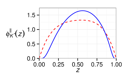
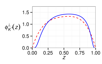
Figure 1: The AdS/QCD DAs (solid blue) compared to the SR DAs (dashed red) at a scale $\mu=2$ GeV.

As for the soft non-perturbative form factors $\xi_{\perp,\parallel}$ appearing in Eqns. (3), (4), (10) and (11), we shall compute them in the heavy quark/large recoil limit. In this limit, the seven $B\to K^{*}$ transition form factors, which we compute using LCSR with AdS/QCD DAs Ahmady et al. (2014), can be expressed in terms of the two soft form factors:

$$A_{1}(E_{K^{*}})=\frac{2E_{K^{*}}}{m_{B}+m_{K^{*}}}\xi_{\bot}(E_{K^{*}}),$$ (33)

$$V(E_{K^{*}})=\frac{m_{B}+m_{K^{*}}}{m_{B}}\xi_{\bot}(E_{K^{*}}),$$ (34)

$$T_{1}(E_{K^{*}})=\xi_{\bot}(E_{K^{*}}),$$ (35)

$$T_{2}(E_{K^{*}})=\frac{2E_{K}^{*}}{m_{B}}\xi_{\bot}(E_{K^{*}}),$$ (36)

$$A_{2}(E_{K^{*}})=\frac{m_{B}}{m_{B}-m_{K^{*}}}\bigg{[}\xi_{\bot}(E_{K^{*}})-\xi_{\|}(E_{K^{*}})\bigg{]},$$ (37)

$$A_{0}(E_{K^{*}})=\frac{E_{K}^{*}}{m_{K}^{*}}\xi_{\|}(E_{K^{*}}),$$ (38)

$$T_{3}(E_{K^{*}})=\xi_{\bot}(E_{K}^{*})-\xi_{\|}(E_{K^{*}}).$$ (39)

Using Eqs. (33), (34), (35) and (36), we do a $3$-parameter fit for $0~{}\mbox{GeV}^{2}\leq q^{2}\leq 8~{}\mbox{GeV}^{2}$ using the parametric form:

$$\xi_{\perp}(q^{2})=\frac{\xi_{\perp}(0)}{1-a\hat{s}+b\hat{s}^{2}}\hskip 28.45274pt\hat{s}=\frac{q^{2}}{m_{B}^{2}}$$ (40)

We compute all the form factors appearing on the left-hand-side of the above equations using the LCSR given in Ref. Aliev et al. (1997). In these LCSR, following Ref. Aliev et al. (1997), we use a Borel parameter $M_{B}=8~{}\mbox{GeV}^{2}$ and a continuum threshold $s_{0}=36~{}\mbox{GeV}^{2}$. Having obtained $\xi_{\perp}$, we are in a position to use Eqs. (37), (38) and (39) to do a similar fit for $\xi_{\parallel}$. The resulting fitted parameters are shown in table 2.

Table 2: Fitted parameters for the soft form factors.

Model	a	b	$\xi_{\perp}(0)$
AdS/QCD	1.662	0.610	0.245
SR	1.599	0.526	0.283

Model	a	b	$\xi_{\parallel}(0)$
AdS/QCD	2.181	1.166	0.076
SR	2.023	0.965	0.076

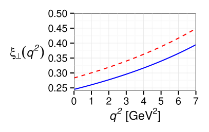
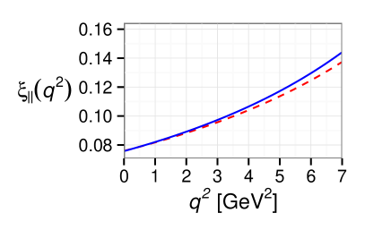
Figure 2: The soft form factors $\xi_{\perp}$ and $\xi_{\parallel}$ as a function of $q^{2}$. Solid blue: AdS/QCD. Dashed red: Sum Rules.

Having specified the DAs and soft form factors, we have now all the ingredients to compute the isospin asymmetry.

IV Results

Before discussing our predictions, let us point out that the integral $X_{\perp}(0)$ in Eq. (14) diverges at the end-point with the SR DA and that we regulate this divergence using a cut-off as in Ref. Feldmann and Matias (2003). The AdS/QCD and Sum Rules predictions for the isospin asymmetry are shown in Fig. 4. The uncertainty band for each prediction is obtained by varying the renormalization scale $\mu_{b}$ between $m_{b}/2$ and $2m_{b}$. As can be seen, our predictions are consistent with the LHCb data in the two lowest $q^{2}$ bins. At higher $q^{2}$, we predict a negative isospin asymmetry while the current LHCb data seem to indicate a positive asymmetry. We note that the theoretical computations of Ref. Feldmann and Matias (2003) and Lyon and Zwicky (2013) also predict a negative asymmetry in this kinematic region.

We extrapolate our predictions down to $q^{2}=0$ in order to update our AdS/QCD prediction Ahmady and Sandapen (2013) of the isospin asymmetry in $B\to K^{*}\gamma$. We obtain an asymmetry of $6.4\%$ in agreement with the PDG average value of $5.2\pm 2.6$ Beringer et al. (2012). Our updated prediction is higher than that ($3.2\%$) obtained in Ref. Ahmady and Sandapen (2013) because of different input parameters and a more careful evaluation of the Wilson coefficients at two different scales as explained earlier in this paper. More importantly, we use our AdS/QCD prediction for the form factor $\xi_{\perp}(0)\approx T_{1}(0)=0.24$ instead of the higher Sum Rules value ($T_{1}(0)=0.31$ Ball et al. (2007a)) used in Ref. Ahmady and Sandapen (2013). Note that our AdS/QCD prediction for $\xi_{\perp}(0)$ is in very good agreement with the empirical estimate $\xi_{\perp}(0)=0.24\pm 0.06$ taken from Ref. Beneke et al. (2001). We note that the Sum Rules prediction slightly overshoots the PDG datum at $q^{2}=0$. We compare our predictions for the asymmetry at $q^{2}=0$ with the available data in Fig. 3.

In Fig. 5, we take a closer look at AdS/QCD and Sum Rules predictions for the isospin asymmetry distribution. As can be seen, the predictions are distinct as $q^{2}\to 0$. Perhaps more interestingly, the predictions become hardly model-dependent and small ($\leq 2.5\%$) for $q^{2}\geq 4~{}\mbox{GeV}^{2}$. At the same time, they are also hardly sensitive to the variation in the renormalization scale. This means that the isospin asymmetry in this kinematic region is indeed a clean observable for investigating New Physics signals. Obviously, more precise data would be necessary to reveal any hints of New Physics.

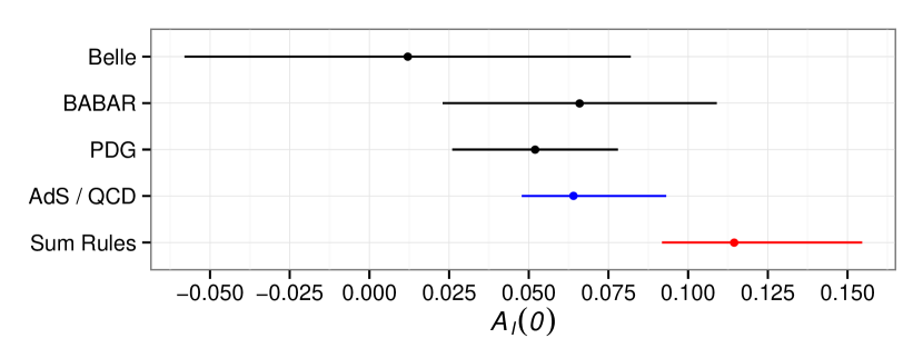
Figure 3: The isospin asymmetry at $q^{2}=0$, i.e. for $B\to K^{*}\gamma$. The AdS/QCD prediction (blue) and the Sum Rules (red) predictions compared to the data from Belle Nakao et al. (2004), BaBar Aubert et al. (2009) and PDG Beringer et al. (2012).

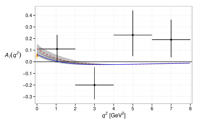
Figure 4: The isospin asymmetry in $B\to K^{*}\mu^{+}\mu^{-}$ as a function of $q^{2}$. The AdS/QCD prediction (solid blue) and the Sum Rules prediction (dashed red) compared to the LHCb data Aaij et al. (2012). The orange square datum from PDG Beringer et al. (2012) is the isospin asymmetry at $q^{2}=0$, i.e. for $B\to K^{*}\gamma$.

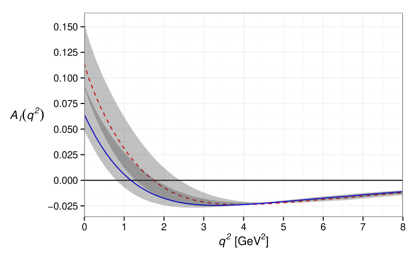
Figure 5: Our predictions for the isospin asymmetry in $B\to K^{*}\mu^{+}\mu^{-}$ as a function of $q^{2}$. Red dashed: Sum Rules. Solid blue: AdS/QCD.

V Conclusions

We have computed the isospin asymmetry in the decay $B\to K^{*}\mu^{+}\mu^{-}$ using Distribution Amplitudes and decay constants for the $K^{*}$ as predicted by AdS/QCD and by Sum Rules. Interestingly, the predictions are hardly model and renormalization scale-dependent in the region of the dimuon mass squared, $q^{2}\geq 4~{}\mbox{GeV}^{2}$, making more precise measurements of this observable in this kinematic region a good probe for New Physics.

VI Acknowledgements

This research is supported by a team grant from the Natural Sciences and Engineering Research Council of Canada (NSERC). SL thanks the government of New-Brunswick through SEED-COOP funding. We thank Robyn Campbell for her input in the initial stage of this research. We thank Tracy Lavoie and Taylor Coady for useful discussions, Raymir Mutua and Liam McManus for reviewing the Appendix.

Appendix A The strong coupling constant: $\alpha_{s}(\mu)$

In this paper, we use the three-loop evolution for $\alpha_{s}(\mu)$:Ahmady and Mahmoudi (2007)

$$\alpha_{s}(\mu)=\frac{4\pi}{\beta_{0}\ln(\mu^{2}/\Lambda^{2})}\left[1-\frac{\beta_{1}}{\beta_{0}^{2}}\frac{\ln(\ln(\mu^{2}/\Lambda^{2}))}{\ln(\mu^{2}/\Lambda^{2})}+\frac{\beta_{1}^{2}}{\beta_{0}^{4}\ln^{2}(\mu^{2}/\Lambda^{2})}\left(\left(\ln(\ln(\mu^{2}/\Lambda^{2}))-\frac{1}{2}\right)^{2}+\frac{\beta_{2}\beta_{0}}{2\beta_{1}^{2}}-\frac{5}{4}\right)\right]$$ (41)

where

$$\beta_{0}=\frac{33-2n_{f}}{3}\hskip 28.45274pt\beta_{1}=\frac{306-38n_{f}}{3}\hskip 28.45274pt\beta_{2}=2857-\frac{5033}{9}n_{f}+\frac{325}{27}n_{f}^{2}$$ (42)

and where $n_{f}$ is the number of active flavors according to which the value of $\Lambda$ is fixed using threshold matching conditions.

Appendix B Wilson Coefficients

We start by computing the “barred” Wilson coefficients $\overline{C}_{1-6}$ used in this paper. The “barred” Wilson coefficients $\overline{C}_{1-6}$ are defined in the basis used in Beneke et al. (2001). By construction, at leading log (LL) accuracy they coincide with the Wilson coefficients $C_{1-6}$ of the standard basis Buras (1998). At next-to-leading log (NLL) accuracy, the two sets of coefficients are related by the equations Beneke et al. (2001)

$$\overline{C}_{i}(\mu)=C_{i}(\mu)+\frac{\alpha_{s}(\mu)}{4\pi}T_{ij}C_{j}(\mu)\hskip 28.45274pti\in\{1,2,3,4,5,6\}$$ (43)

where

$$T_{ij}=\left(\begin{array}[]{cccccc}\frac{7}{3}&2&0&0&0&0\\ 1&-\frac{2}{3}&0&0&0&0\\ 0&0&-\frac{178}{27}&-\frac{4}{9}&\frac{160}{27}&\frac{13}{9}\\ 0&0&\frac{34}{9}&\frac{20}{3}&-\frac{16}{9}&-\frac{13}{3}\\ 0&0&\frac{164}{27}&\frac{23}{9}&-\frac{146}{27}&-\frac{32}{9}\\ 0&0&-\frac{20}{9}&-\frac{23}{3}&\frac{2}{9}&\frac{16}{3}\end{array}\right)$$ (44)

The NLL coefficients $C_{1-6}$ are themselves given by Buras (1998):

$$C_{i}(\mu)=C_{i}^{0}(\mu)+\frac{\alpha_{s}(\mu)}{4\pi}C_{i}^{1}(\mu)$$ (45)

where

$$C_{i}^{0}(\mu)=\sum_{j=1}^{8}k_{ij}\eta^{a_{j}}\hskip 28.45274ptC_{i}^{1}(\mu)=\sum_{j=1}^{8}(e_{ij}\eta E_{0}(x_{t})+f_{ij}+g_{ij}\eta)\eta^{a_{j}}$$ (46)

with

$$\eta=\frac{\alpha_{s}(m_{W})}{\alpha_{s}(\mu)}\hskip 28.45274ptE_{0}(x)=\frac{x(18-11x-x^{2})}{12(1-x)^{3}}+\frac{x^{2}(15-16x+4x^{2})}{6(1-x)^{4}}\ln(x)-\frac{2}{3}\ln(x)$$ (47)

andAhmady and Mahmoudi (2007)

$$x_{t}=\frac{\overline{m_{t}}(m_{W})^{2}}{m_{W}^{2}}\;.$$ (48)

In Eq. (48), the running top mass is given by

$$\overline{m_{t}}(\mu)=\overline{m_{t}}(m_{t})\left(\frac{\alpha_{s}(\mu)}{\alpha_{s}(m_{t})}\right)^{\frac{\gamma_{0}^{m}}{2\beta_{0}}}\left(1+\frac{\alpha_{s}(m_{t})}{4\pi}\frac{\gamma_{0}^{m}}{2\beta_{0}}\left(\frac{\gamma_{1}^{m}}{\gamma_{0}^{m}}-\frac{\beta_{1}}{\beta_{0}}\right)\left(\frac{\alpha_{s}(\mu)}{\alpha_{s}(m_{t})}-1\right)\right)$$ (49)

where ($m_{t}$ is the pole mass of the top quark)

$$\overline{m_{t}}(m_{t})=m_{t}\left(1-\frac{4}{3}\frac{\alpha_{s}(m_{t})}{\pi}\right)\hskip 28.45274pt\gamma_{0}^{m}=8\hskip 28.45274pt\gamma_{1}^{m}=\frac{404}{3}-\frac{40}{9}n_{f}$$ (50)

To completely specify (46), we also need the following matrices:

$$k_{ij}=\left(\begin{array}[]{cccccccc}0&0&\frac{1}{2}&-\frac{1}{2}&0&0&0&0\\ 0&0&\frac{1}{2}&\frac{1}{2}&0&0&0&0\\ 0&0&-\frac{1}{14}&\frac{1}{6}&0.0510&-0.1403&-0.0113&0.0054\\ 0&0&-\frac{1}{14}&-\frac{1}{6}&0.0984&0.1214&0.0156&0.0026\\ 0&0&0&0&-0.0397&0.0117&-0.0025&0.0304\\ 0&0&0&0&0.0335&0.0239&-0.0462&-0.0112\end{array}\right)$$ (51)

$$e_{ij}=\left(\begin{array}[]{cccccccc}0&0&0&0&0&0&0&0\\ 0&0&0&0&0&0&0&0\\ 0&0&0&0&0.1494&-0.3726&0.0738&-0.0173\\ 0&0&0&0&0.2885&0.3224&-0.1025&-0.0084\\ 0&0&0&0&-0.1163&0.0310&0.0162&-0.0975\\ 0&0&0&0&0.0982&0.0634&0.3026&0.0358\end{array}\right)$$ (52)

$$f_{ij}=\left(\begin{array}[]{cccccccc}0&0&0.8136&0.7142&0&0&0&0\\ 0&0&0.8136&-0.7142&0&0&0&0\\ 0&0&-0.0766&-0.1455&-0.8848&0.4137&-0.0114&0.1722\\ 0&0&-0.2353&-0.0397&0.4920&-0.2758&0.0019&-0.1449\\ 0&0&0.0397&0.0926&0.7342&-0.1262&-0.1209&-0.1085\\ 0&0&-0.1191&-0.2778&-0.5544&0.1915&-0.2744&0.3568\end{array}\right)$$ (53)

$$g_{ij}=\left(\begin{array}[]{cccccccc}0&0&1.0197&2.9524&0&0&0&0\\ 0&0&1.0197&-2.9524&0&0&0&0\\ 0&0&-0.1457&-0.9841&0.2303&1.4672&0.0971&-0.0213\\ 0&0&-0.1457&0.9841&0.4447&-1.2696&-0.1349&-0.0104\\ 0&0&0&0&-0.1792&-0.1221&0.0213&-0.1197\\ 0&0&0&0&0.1513&-0.2497&0.3983&0.0440\end{array}\right)$$ (54)

and Buchalla et al. (1996)

$$a_{i}=\left(\begin{array}[]{cccccccc}\frac{14}{23}&{16}{23}&\frac{6}{23}&-\frac{12}{23}&0.4086&-0.4230&-0.8994&0.1456\end{array}\right)$$ (55)

We now turn to the computation of the Wilson coefficients $C_{7,8}^{\rm eff}$. At NLL accuracy, they are given by

$$C_{7,8}^{\rm eff}(\mu)=C_{7,8}^{(0)\rm eff}(\mu)+\frac{\alpha_{s}(\mu)}{4\pi}C_{7,8}^{(1)\rm eff}(\mu)$$ (56)

where Buras (1998)

$$C_{7}^{(0)\rm eff}(\mu)=\eta^{\frac{16}{23}}C_{7}^{(0)}(m_{W})+\frac{8}{3}\left(\eta^{\frac{14}{23}}-\eta^{\frac{16}{23}}\right)C_{8}^{(0)}(m_{W})+C_{2}^{(0)}(m_{W})\sum_{i=1}^{8}h_{i}\eta^{a_{i}}\;,$$ (57)

and

$$C_{7}^{(1)\rm eff}(\mu)=\eta^{\frac{39}{23}}C_{7}^{(1)\rm eff}(m_{W})+\frac{8}{3}\left(\eta^{\frac{37}{23}}-\eta^{\frac{39}{23}}\right)C_{8}^{(1)\rm eff}(m_{W})\\ +\left(\frac{297664}{14283}\eta^{\frac{16}{23}}-\frac{7164416}{357075}\eta^{\frac{14}{23}}+\frac{256868}{14283}\eta^{\frac{37}{23}}-\frac{6698884}{357075}\eta^{\frac{39}{23}}\right)C_{8}^{(0)}(m_{W})\\ +\frac{37208}{4761}\left(\eta^{\frac{39}{23}}-\eta^{\frac{16}{23}}\right)C_{7}^{(0)}(m_{W})+\sum_{i=1}^{8}(e^{\prime}_{i}\eta E_{0}(x_{t})+f^{\prime}_{i}+g^{\prime}_{i}\eta)\eta^{a_{i}}\;,$$ (58)

while

$$C_{8}^{(0)\rm eff}(\mu)=\eta^{\frac{14}{23}}C_{8}^{(0)}(m_{W})+C_{2}^{(0)}(m_{W})\sum_{i=1}^{8}\overline{h}_{i}\eta^{a_{i}}\;.$$ (59)

and Greub and Liniger (2001)

$$C_{8}^{(1)\rm eff}(\mu)=\eta^{\frac{37}{23}}C_{8}^{(1)\rm eff}(m_{W})+6.7441\left(\eta^{\frac{37}{23}}-\eta^{\frac{14}{23}}\right)C_{8}^{(0)}(m_{W})\\ +\sum_{i=1}^{8}\left(\overline{e^{\prime}}_{i}\eta C_{4}^{(1)\rm eff}(m_{W})+\left(\overline{f^{\prime}}_{i}+\overline{g^{\prime}}_{i}\eta\right)C_{2}^{(0)}(m_{W})+\overline{l^{\prime}}_{i}\eta C_{1}^{(1)\rm eff}(m_{W})\right)\eta^{a_{1}}\;.$$ (60)

The various Wilson coefficient at a scale $m_{W}$ are given below: Greub and Liniger (2001)

$$C_{1}^{(1)\rm eff}(m_{W})=15\hskip 28.45274ptC_{2}^{(0)}(m_{W})=1\hskip 28.45274ptC_{4}^{(1)\rm eff}(m_{W})=E_{0}(x_{t})-\frac{2}{3}$$ (61)

whileBuras (1998)

$$C_{7}^{(0)}(m_{W})=\frac{3x_{t}^{3}-2x_{t}^{2}}{4(x_{t}-1)^{4}}\ln(x_{t})+\frac{-8x_{t}^{3}-5x_{t}^{2}+7x_{t}}{24(x_{t}-1)^{3}}$$ (62)

$$C_{7}^{(1)\rm eff}(m_{W})=\frac{-16x_{t}^{4}-122x_{t}^{3}+80x_{t}^{2}-8x_{t}}{9(x_{t}-1)^{4}}\operatorname{Li}_{2}\left(1-\frac{1}{x_{t}}\right)+\frac{6x_{t}^{4}+46x_{t}^{3}-28x_{t}^{2}}{3(x_{t}-1)^{5}}\ln^{2}x_{t}\\ +\frac{-102x_{t}^{5}-588x_{t}^{4}-2262x_{t}^{3}+3244x_{t}^{2}-1364x_{t}+208}{81(x_{t}-1)^{5}}\ln(x_{t})\\ +\frac{1646x_{t}^{4}+12205x_{t}^{3}-10740x_{t}^{2}+2509x_{t}-436}{486(x_{t}-1)^{4}}$$ (63)

$$C_{8}^{(0)}(m_{W})=\frac{-3x_{t}^{2}}{4(x_{t}-1)^{4}}\ln(x_{t})+\frac{-x_{t}^{3}+5x_{t}^{2}+2x_{t}}{8(x_{t}-1)^{3}}$$ (64)

$$C_{8}^{(1)\rm eff}(m_{W})=\frac{-4x_{t}^{4}+40x_{t}^{3}+41x_{t}^{2}+x_{t}}{6(x_{t}-1)^{4}}\operatorname{Li}_{2}\left(1-\frac{1}{x_{t}}\right)+\frac{-17x_{t}^{3}-31x_{t}^{2}}{2(x_{t}-1)^{5}}\ln^{2}(x_{t})\\ +\frac{-210x_{t}^{5}+1086x_{t}^{4}+4893x_{t}^{3}+2857x_{t}^{2}-1994x_{t}+280}{216(x_{t}-1)^{5}}\ln(x_{t})\\ +\frac{737x_{t}^{4}-14102x_{t}^{3}-28209x_{t}^{2}+610x_{t}-508}{1296(x_{t}-1)^{4}}$$ (65)

where $\operatorname{Li}_{2}(z)$ is Spence’s function defined by

$$\operatorname{Li}_{2}(z)=-\int_{0}^{z}\frac{\ln(1-u)}{u}du$$ (66)

i	1	2	3	4	5	6	7	8
$e^{\prime}$	$\frac{4661194}{816831}$	$-\frac{8516}{2217}$	0	0	-1.9043	-0.1008	0.1216	0.0183
$f^{\prime}$	-17.3023	8.5027	4.5508	0.7519	2.0040	0.7476	-0.5385	0.0914
$g^{\prime}$	14.8088	-10.8090	-0.8740	0.4218	-2.9347	0.3971	0.1600	0.0225
$h$	2.2996	-1.0880	$-\frac{3}{7}$	$-\frac{1}{14}$	-0.6494	-0.0380	-0.0185	-0.0057
$\overline{e^{\prime}}$	2.1399	0	0	0	-2.6788	0.2318	0.3741	-0.0670
$\overline{f^{\prime}}$	-5.8157	0	1.4062	-3.9895	3.2850	3.6851	-0.1424	0.6492
$\overline{g^{\prime}}$	3.7264	0	0	0	-3.2247	0.3359	0.3812	-0.2968
$\overline{l^{\prime}}$	0.2169	0	0	0	-0.1793	-0.0730	0.0240	0.0113
$\overline{h}$	0.8623	0	0	0	-0.9135	0.0873	-0.0571	0.0209

Table 3: Useful numbers in the calculation of $C_{7}^{\rm eff}$ and $C_{8}^{\rm eff}$

Finally, we compute the Wilson coefficients $C_{9}$ and $C_{10}$ at NLL using Buchalla et al. (1996)

$$C_{9}(\mu)=P_{0}+\frac{Y_{0}(x_{t})}{\sin^{2}(\theta_{W})}-4Z_{0}(x_{t})+P_{E}E_{0}(x_{t})$$ (67)

where $\theta_{W}$ is the Weinberg angle (i.e. $\sin^{2}(\theta_{W})=0.23$) and the functions $P_{0}$, $P_{E}$, $Y_{0}$ and $Z_{0}$ are given by:

$$P_{0}=\frac{\pi}{\alpha_{s}(m_{W})}(-0.1875+\sum_{i=1}^{8}p_{i}\eta^{a_{i}+1})+1.2468+\sum_{i=1}^{8}\eta^{a_{i}}(r_{i}+s_{i}\eta)$$ (68)

$$P_{E}=0.1405+\sum_{i=1}^{8}q_{i}\eta^{a_{i}+1}$$ (69)

$$Y_{0}(x)=C_{0}(x)-B_{0}(x)\hskip 28.45274ptZ_{0}=C_{0}+\frac{1}{4}D_{0}(x)$$ (70)

where the functions $B_{0}$, $C_{0}$ and $D_{0}$ are defined by:

$$B_{0}(x)=\frac{1}{4}\left(\frac{x}{1-x}+\frac{x\ln(x)}{(x-1)^{2}}\right)\hskip 28.45274ptC_{0}(x)=\frac{x}{8}\left(\frac{x-6}{x-1}+\frac{3x+2}{(x-1)^{2}}\ln(x)\right)$$ (71)

$$D_{0}(x)=-\frac{4}{9}\ln(x)+\frac{-19x^{3}+25x^{2}}{36(x-1)^{3}}+\frac{x^{2}(5x^{2}-2x-6)}{18(x-1)^{4}}\ln(x)$$ (72)

The $C_{10}$ Wilson coefficient has no scale dependenceBuchalla et al. (1996):

$$C_{10}(\mu)=C_{10}(m_{W})=-\frac{Y_{0}(x_{t})}{\sin^{2}(\theta_{W})}\;.$$ (73)

i	1	2	3	4	5	6	7	8
$p$	0	0	$-\frac{80}{203}$	$\frac{8}{33}$	0.0433	0.1384	0.1648	-0.0073
$r$	0	0	0.8966	-0.1960	-0.2011	0.1328	-0.0292	-0.1858
$s$	0	0	-0.2009	-0.3579	0.0490	-0.3616	-0.3554	0.0072
$q$	0	0	0	0	0.0318	0.0918	-0.2700	0.0059

Table 4: Useful numbers in the calculation of $C_{9}$.