BICEP’s acceleration

Abstract

The recent Bicep2 bicep2 detection of, what is claimed to be primordial $B$-modes, opens up the possibility of constraining not only the energy scale of inflation but also the detailed acceleration history that occurred during inflation. In turn this can be used to determine the shape of the inflaton potential $V(\phi)$ for the first time - if a single, scalar inflaton is assumed to be driving the acceleration. We carry out a Monte Carlo exploration of inflationary trajectories given the current data. Using this method we obtain a posterior distribution of possible acceleration profiles $\epsilon(N)$ as a function of $e$-fold $N$ and derived posterior distributions of the primordial power spectrum $P(k)$ and potential $V(\phi)$. We find that the Bicep2 result, in combination with Planck measurements of total intensity Cosmic Microwave Background (CMB) anisotropies, induces a significant feature in the scalar primordial spectrum at scales $k\sim 10^{-3}$ Mpc^-1. This is in agreement with a previous detection of a suppression in the scalar power Contaldi .

I Introduction

The recent Bicep2 detection bicep2 of curl patterns, apparently primordial in nature, in the CMB polarisation pattern, ushers in a new era in the search for a “complete theory” of the early Universe. Curl or $B$-type modes can only be induced in the polarisation by either tensor modes - a background of gravitational waves present at last scattering, or by lensing due to structure along the line of sight that distorts gradient modes ($E$-type) into curl modes. The only other possible source of $B$-modes, unless new physics is invoked, is foreground contamination but Bicep2 claims to have ruled out this possibility with some level of confidence.

In turn, a confirmation that a relic background of super horizon scaled gravitational waves was present at last scattering will lend very strong support to the idea that an epoch of inflation occurred in the very early Universe. A gravitational wave background is a nearly unavoidable consequence of a period of quasi de Sitter expansion in the early Universe if it was driven by a single scalar field Grishchuk:1974ny ; Starobinsky:1979ty ; Rubakov:1982df ; Fabbri:1983us ; Abbott:1984fp . The amplitude observed by Bicep2 is close to that predicted by simple inflationary models such as chaotic inflation Linde:1983gd and natural inflation Freese:1990rb .

On the other hand the tensor-to-scalar ratio $r=0.2$ that fits best the Bicep2 data is in tension with constraints arising from total intensity CMB measurements wmap ; planck on large angular scales. The total intensity on scales larger than the sound horizon at last scattering is a sum of both scalar and tensor contributions. A measurement of the total and fits to the $\Lambda$CDM model with power law primordial spectra results in a limit on $r$ with $r<0.11$ at 95% confidence. This has led to some speculation of non-standard behaviour at large scales Contaldi and/or the requirement of running of the spectral index and non-standard physics on smaller scales (see for example smith ).

In Contaldi we noted that a simple suppression of the scalar power on scales $k\sim 10^{-3}$ Mpc^-1 easily achieves a reconciliation of the Bicep2 and Planck spectra without creating additional tension with other small scale probes. This is in contrast to the addition of curvature to the primordial spectrum, also known as running of the spectral index. This has two disadvantages; the first is that the required running is some two orders of magnitude larger than what is expected in the simplest models of inflation. The second is that the addition of a curvature term modifies the spectrum on all scales and will lead to tension with observations on smaller scales from Large Scale Structure (LSS) surveys.

The required suppression, some 25% in power, can be achieved in simple modifications of the single inflaton field paradigm such as the Starobinsky model starobinski as shown in Contaldi . Here we take a model independent approach to analysing the data by considering the parametrisation of the acceleration history during inflation as modes observable today were exiting the horizon. This is in contrast to the standard method that assumes $d\ln P(k)/d\ln k$ is well described by a Taylor expansion involving the spectral index $n_{s}$, a running $dn_{s}/d\ln k$, etc. or methods parametrising whole classes of inflation models (see for example barranco ).

Given a suitable parametrisation of the acceleration we can then obtain its posterior distribution with respect to observations via Monte Carlo exploration of the data likelihoods. This in turn allows us to derive constraints on the primordial spectra and the inflationary potential if we make model dependent assumptions relating the power spectra to the original inflaton field perturbations.

This paper is organised as follows. In section II we describe the formalism for generating observables via the parametrisation of the acceleration occurring during inflation. In section III we describe the sampling method used in our MCMC exploration of the likelihoods using the parametrised acceleration formalism. In section IV we show the results of various runs and compare to conventional fits to the data generated by parametrising the primordial power spectra as power laws and power laws with running of the spectral index. We obtain posterior distributions for the acceleration trajectories and its derived corollaries - the scalar primordial spectrum and inflationary potential. We discuss our results in section V.

II Method

Assuming a Friedmann-Robertson-Walker background with scale factor $a(t)$ evolving with cosmological time $t$ the background evolution is described completely by the Hubble rate $H=\dot{a}/a$ and the quantity $\epsilon$ which is a measure of the acceleration in $a$

$$\epsilon=-\frac{\dot{H}}{H^{2}}\equiv 1-\frac{\ddot{a}}{a}\,,$$ (1)

where $H=\dot{a}/a$ and overdots represent derivatives with respect to time $t$. By definition when $\epsilon<1$ the rate of change of $a$ is increasing and the Universe is inflating. When $\epsilon\ll 1$ the Hubble rate is nearly constant and the background is close to de Sitter or in the “slow-roll” regime as long as higher derivatives of $H$ are also small.

For convenience it is useful to switch independent variable to $e$-folds defined as $N=\ln a/a_{0}$. Given a background history or “trajectory” in $H(N)$ and $\epsilon(N)$ we can define observable quantities. For example, to first order in the slow-roll expansion lyth , the resulting primordial curvature and tensor mode dimensionless spectra are given by

$$k^{3}P_{s}(k)=\left.A_{s}\,\frac{H^{2}(N)}{\epsilon(N)}\right|_{N=N_{k}}\,,$$ (2)

and

$$k^{3}P_{t}(k)=\left.16\,A_{s}\,H^{2}(N)\right|_{N=N_{k}}\,,$$ (3)

respectively. Here $N_{k}$ is the $e$-fold at which mode with fourier wavenumber $k$ exits the horizon with $k=aH$ and $A_{s}$ is the primordial normalisation of the perturbations. The ratio of the two spectra

$$r(N)\equiv\frac{P_{t}}{P_{s}}=16\,\epsilon(N)\,,$$ (4)

is often quoted, at a chosen pivot scale, as the model defining observable as in the Bicep2 case.

Parameter	Prior range	Definition
$\omega_{b}\equiv\Omega_{b}\,h^{2}$	[0.005,0.1]	Baryon density today
$\omega_{c}\equiv\Omega_{c}\,h^{2}$	[0.001,0.99]	Cold dark matter density today
$100\,\theta_{MC}$	[0.5,10.0]	100 $\times$ CosmoMC sound horizon to angular diameter distance ratio approximation
$\tau$	[0.01,0.8]	Optical depth to reionisation
$\ln(10^{10}A_{s})$	[2.7 4]	Scalar spectrum normalisation
$\ln\epsilon_{i}$	[-11.5,-1.6]	Number of $e$-folds for which trajectory is integrated back from end of inflation
$n_{s}(k_{\star})$	…	Scalar spectral index measured from trajectory spectrum at scale $k_{\star}=0.05$ Mpc-1
$r(k_{\star})$	…	Tensor-to-scalar ratio measured from trajectory spectra at scale $k_{\star}=0.05$ Mpc-1

Table 1: Uniform MCMC priors for cosmological parameters and their descriptions. Planck nuisance parameters are not listed here but are included with the same prior settings as used in planck_pars . The second block are derived parameters that are not sampled directly.

Both these spectra source anisotropies in the total intensity of the CMB but only the tensor spectra sources the $B$-modes of the polarisation. In both cases the tensor contribution is negligible beyond multipoles $\ell\sim 200$ as gravitational waves decay once they re-enter the horizon and only modes that were larger than the horizon scale at recombination affect the pattern of anisotropies.

Assuming a single scalar field $\phi$ rolling down a potential $V(\phi)$ is driving inflation the Hubble equation is given by

$$H^{2}=\frac{1}{3M_{\rm pl}^{2}}\left(\frac{1}{2}\dot{\phi}^{2}+V(\phi)\right)\,,$$ (5)

where $M_{\rm pl}$ is the reduced Planck mass. The inflaton equation of motion is

$$\ddot{\phi}+3H\dot{\phi}+\frac{\partial V}{\partial\phi}=0\,.$$ (6)

These can be combined to relate $\epsilon$ to the time derivative of the inflaton

$$\epsilon=\frac{1}{2M_{\rm pl}^{2}}\left(\frac{\dot{\phi}}{H}\right)^{2}\,.$$ (7)

The above can then be substituted back into (5) to obtain a relationship between $\epsilon$, $H$ and the scalar potential

$$V[\epsilon(N)]=3M^{2}_{pl}H^{2}(N)\left[1-\frac{\epsilon(N)}{3}\right]\,.$$ (8)

In turn this can be used to reconstruct $V[\phi(N)]$ by relating $\phi$ to $\epsilon(N)$ via (7)

$$\phi(N)-\phi_{0}=-\sqrt{2}\int^{N}_{0}\sqrt{\epsilon(\tilde{N})}\,d\tilde{N}\,.$$ (9)

At any time ($e$-fold) the Hubble rate can be obtained, up to a normalisation, by integrating $\epsilon$ too

$$\ln H(N)-\ln H_{0}=-\int^{N}_{0}\epsilon(\tilde{N})\,d\tilde{N}\,.$$ (10)

Similarly the scale of the mode exiting the horizon at each $e$-fold can be calculated using $k=aH$

$$\ln k(N)-\ln k_{0}=N+\ln H(N)=N-\int^{N}_{0}\epsilon(\tilde{N})\,d\tilde{N}\,.$$ (11)

The implicit assumption made in (11) is that we know the exact number of $e$-folds that occurred after the Universe stopped inflating. This is sensitive to the exact evolution of the background during the reheating epoch which would shift the relation between $\ln k$ and $N$ systematically by a few $e$-folds. We will ignore this unknown shift when relating $e$-folds to observable scales.

Thus, assuming first order in slow-roll, all quantities required to compute observables can be calculated by specifying the function $\epsilon(N)$ and a normalisation scale $A_{s}$.

III Sampling the acceleration

In our method the functional space $\epsilon(N)$ is the basis for the Markov Chain Monte Carlo (MCMC) exploration of data likelihoods. We sample the space by drawing random amplitudes in $\ln\epsilon$ at a series of regularly spaced spline $e$-folds $N_{i}$. The spline points are then used to reconstruct the full function $\epsilon(N)$ using a cubic spline numrec .

A cubic spline ensures a sufficiently smooth function for our purposes and the sampling of $\ln\epsilon$ ensures that we always obtain an inflating solution with $H$ decreasing monotonically with time or $e$-fold. Our use of the first order slow roll approximation also means that we only need to integrate the splined function to obtain the spectra and scale definitions. If higher orders or the full, numerical solutions, were required the derivatives of the function $\epsilon(N)$ would have to be defined. This would require a higher order interpolation scheme and more parameters to have $d^{2}\epsilon/dN^{2}$ be continuous and compute quantities to second order in slow roll.

First order in slow roll may seem restrictive in the context of exploring structure in the inflationary trajectories but the data is suggesting a transition between two regimes that are well within the slow roll approximation Contaldi and this should therefore be sufficient to define the trajectories in the observational window.

We use the CosmoMC package cosmomc for the MCMC exploration and modify it to search in the space of spline point amplitudes $\epsilon_{i}$ where $i=1,...,N_{\rm sp}$ instead of the usual primordial parameters $n_{s}$, $r$, $dn_{s}/d\ln k$, $n_{t}$, etc. The spline points are positioned regularly between $N=0$ and $N=N_{\rm max}$ corresponding to the largest and smallest modes $k$ required by the CAMB package camb in order to compute the CMB spectra between multipoles $2\leq\ell\leq 2500$. The range of scales required, typically ${\cal O}(10^{-5})\leq k\leq{\cal O}(10^{-1})$, extends well beyond the range where CMB observations have a significant impact but are required in order to integrate the radiation transfer functions to a sufficient degree of accuracy. Thus the regular spacing in such a wide range is not optimal but it avoids the need to extrapolate the functions beyond the range covered by our splining.

At each MCMC sample we compute the cubic spline of the $\epsilon_{i}$ amplitudes to obtain a continuous function $\epsilon(N)$ in the chosen range. This function is integrated to obtain $H(N)$, the corresponding scales $\ln k(N)$, and the inferred value of the field $\phi$. The scalar and tensor primordial power spectrum are then calculated using (2) and (3) respectively. These are then passed onto CAMB for convolution with the CMB radiation transfer functions.

The cubic spline method requires an assumption for the derivatives at the boundaries and we adopt the “natural spline” assumption by imposing that the curvature vanishes at the boundaries i.e. that the gradient is constant.

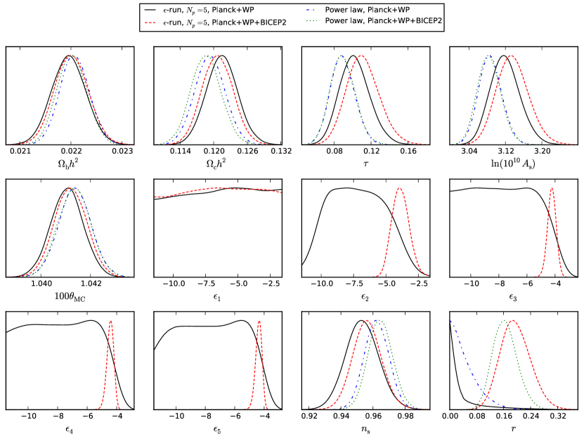
Figure 1: 1-d marginalised posteriors for the ten basic and two ($n_{s}$ and $r$) derived parameters. The $\epsilon$ runs are all for $N_{\rm sp}=5$ and are compared to the power law model runs for data combinations including and excluding Bicep2. In the no Bicep2 case the $\epsilon$ spline point amplitudes are not constrained although the significant correlation between each spline point results in functions with tilts that are still compatible with observations.

We run CosmoMC as setup for Planck data runs. These include a number of Planck nuisance parameters that are used to marginalise over systematic or astrophysical residuals in the Planck spectra. The data combination also includes WMAP polarisation and we label this “Planck+WP”. In addition to this we include the Bicep2 results as provided in the most recent CosmoMC release. Uniform priors for all nuisance parameters are left unchanged from the standard Planck runs.

Table 1 gives a summary of the uniform priors assumed for cosmological parameters and lists the definitions of the derived parameters $n_{s}$ and $r$ used to compare with conventional runs assuming power law spectra. The derived parameters are calculated using the first order slow-roll approximations

$$n_{s} = 1-4\epsilon+2\eta\,,$$

$$r = 16\epsilon\,,$$ (12)

$$n_{t} = -2\epsilon\,,$$

where $\eta=\epsilon-d\ln\epsilon/dN$ and is calculated analytically from the cubic spline for $\ln\epsilon$.

The MCMC chains are run until the $R^{-1}$ convergence parameter is smaller than 0.01. We run cases with $N_{\rm sp}$=5, 6, and 7. For $N_{\rm sp}>7$ the MCMC sampling becomes very inefficient and the required convergence criterion is difficult to achieve due to the large correlations between the $\epsilon_{i}$ spline point amplitudes. A typical run with eight parallel chains contains several hundred thousand accepted models. The minimal case, with $N_{\rm sp}=5$, includes two boundary points and three internal points so should be able to fit the data at least as well as spectral models with three or four parameters e.g. $n_{s}$, $r$, $dn_{s}/d\ln k$, and an (independent) $n_{t}$.

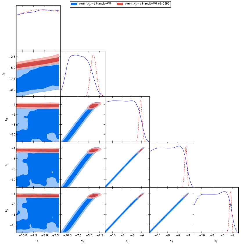
Figure 2: Triangle plot showing the 2-d marginalised posteriors for the spline point amplitudes in the $N_{\rm sp}$ run. The contours indicate 68% and 95% confidence regions and we compare the case with and without Bicep2 included. When Bicep2 is included the spline point amplitudes are tightly constrained although the smaller scale points $\epsilon_{4}$ and $\epsilon_{5}$ are very correlated. This is driven by high-$\ell$ CMB observations tightly constraining the allowed gradient on small scales.

IV Results

IV.1 Acceleration

Model	Data	$\Delta N_{p}$	$\Delta\chi^{2}$	$\Delta\mbox{\sl AIC}$	Rel. Like
Power law	P+WP	0	–	-0.066	0.968
$\epsilon$ $N_{\rm sp}=5$	P+WP	+3	-6.070	–	1.000
Power law	P+WP+B2	0	–	-4.920	0.085
Running	P+WP+B2	+1	-6.68	-2.42	0.785
$\epsilon$, $N_{\rm sp}=5$	P+WP+B2	+3	-10.92	–	1.000
$\epsilon$, $N_{\rm sp}=6$	P+WP+B2	+4	-12.50	-0.422	0.810
$\epsilon$, $N_{\rm sp}=7$	P+WP+B2	+5	-12.22	-2.704	0.259

Table 2: Best-fit $\chi^{2}$ values for the various $\epsilon$ runs compared to standard, power law runs with (P+WP+B2 ) and without Bicep2 (P+WP) data. $\Delta N_{p}$ is the change in total number of model parameters compared to the power law case which has $N_{p}=21$ (7 cosmological + 14 nuisance) parameters and the case including running of the spectral index. The relative likelihood is evaluated using the Akaike Information Criterion (AIC) with respect to the model in both data combination that gives the lowest AIC value. We see that when Bicep2 is absent the $\epsilon$ model is not favoured significantly over the power law model. When Bicep2 is included the power law model has a relatively likelihood of only 8.5% with respect to the $N_{\rm sp}=5$ $\epsilon$ model. We can also conclude that the $N_{\rm sp}=5$ model is slightly more motivated than the power law + running case i.e. it is just as motivated by the data as a solution to the tension.

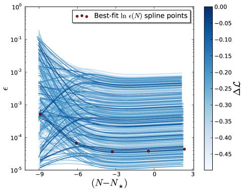
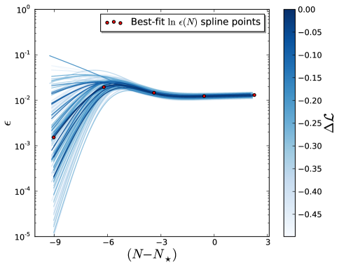
Figure 3: Ensemble of splined trajectories that lie within $|\Delta{\cal L}|<0.5$ from the best-fit model in the $N_{\rm sp}=5$ case excluding (top) and including (bottom) the Bicep2 data. Each $\epsilon$ trajectory is colour coded by distance from the best-fit. The (red) points show the spline point amplitudes for the best-fitting trajectory. The range in $e$-folds is shifted with $N_{\star}$ corresponding to the $e$-fold at which the scale $k=0.05$ Mpc^-1 exited the horizon.

We start by looking at the minimal $N_{\rm sp}=5$ run. In Figure 1 we show the marginalised posterior distribution for the 10 cosmological parameters and two derived parameters, $n_{s}$ and $r$. We compare the Planck+WP and Planck+WP+Bicep2 data combinations for both $\epsilon$ and power law runs. The $\epsilon$ spline point amplitudes are largely unconstrained when Bicep2 is not included. Despite this the posterior in $n_{s}$ is well constrained in the $\epsilon$ runs. This is due to the fact that although the amplitude is unconstrained for any particular trajectory it is highly correlated with its gradient ($\eta$) and the combination is fixed by the data. When Bicep2 is included all spline points except the first one are well constrained. This is due to the measurement of tensor mode amplitude which fixes $\epsilon$ directly.

The posterior in $r$ is consistent with zero in both cases without Bicep2 data. The difference in shape of the posterior is driven by our $\ln\epsilon\equiv\ln r$ prior versus the linear prior used in the conventional power law run. When Bicep2 is included the posteriors are similar and the choice of prior is not a dominant factor anymore since the detection is significant. However is does affect the location of the peak in the posterior and that of correlated variables $\tau$ and $A_{s}$.

The correlations between spline point amplitudes in the two $\epsilon$ runs are shown in Figure 2. We see that the spline points at higher $N$, corresponding to modes exiting the horizon later in inflation, are highly correlated due to the tightly constrained tilt of the CMB anisotropies at high-$\ell$ as observed by Planck. This also explains why the last spline point amplitude, corresponding to a scale of $\sim 0.1$ Mpc^-1 is apparently well constrained despite the fact that CMB observations by Planck do not extend to those scales.

Figure 3 shows the ensemble of splined $\epsilon$ trajectories in the $N_{\rm sp}=5$ for the Planck+WP and Planck+WP+Bicep2 data combinations. The trajectories are selected from the MCMC chains to be within 0.5 in log likelihood ${\cal L}$ from the best-fitting trajectory. This would be equivalent to the 1-$\sigma$ set if the likelihood were Gaussian. There are 250 trajectories within this range of $\Delta{\cal L}$ for the accepted MCMC steps in the chain. Each curve is colour coded according to the $\Delta{\cal L}$ value of its fit to the data (Planck+WP+Bicep2). We see that the shape of $\epsilon(N)$ is well constrained in both cases (with and without Bicep2). However its amplitude is not well constrained when Bicep2 data is absent since a direct measurement if $\epsilon$ is not possible unless $B$-modes are detected. At later times (larger $N$) the combination of Bicep2 and Planck’s high-$\ell$ CMB observations tightly focus $\epsilon(N)$. The small, positive gradient in this regime gives rise to the slightly red tilted ($n_{s}<1$) scalar spectrum. At early times the function is essentially unconstrained but this region does not affect the observables. The rise in amplitude at $N-N_{\star}\sim-5$ will cause a suppression of the scalar power since $H$ is approximately constant and the power is proportional to the inverse of $\epsilon$. This is the feature which has been noted in the literature and is driven by the Planck vs Bicep2 tension.

In Table 2 we show a summary of the model comparisons between the power law assumption and $N_{\rm sp}=5$, 6, and 7 runs. We quote both $\Delta\chi^{2}$ values for the best-fitting models in each MCMC chain and the Akaike Information Criterion (AIC) assessment of their relative likelihoods AIC .

The AIC is defined as AIC $=2\,N_{p}+\chi^{2}$, where $N_{p}$ is the number of parameters in the model. It attempts to properly take into account the penalty for using models with increasing number of parameters to describe a set of data. The relative likelihood between a model with minimum AIC value and a second model

$$L_{\mbox{\sl AIC}}=\exp\left[(\mbox{\sl AIC}_{\mbox{min}}-\mbox{\sl AIC})/2\right]\,,$$ (13)

gives an estimate of the probability that the second model minimizes the information required to describe the data over the first one. $N_{p}=21$ for the tensor, power law model run including the Planck data - 7 cosmological parameters and 14 nuisance parameters.

We see that the $\epsilon$ model with $N_{\rm sp}=5$ uses the minimum information to describe the data compared to all other models considered. It is comparable to the power law + running case in this aspect. However if higher-$\ell$ data or LSS constraints were to be added the relative likelihood of the running model would drop significantly due to tight limits on the running from small scales. Thus the $\epsilon$ model is favoured by the data and this is driven almost entirely by the Bicep2 data since the likelihoods are not significantly different in the no Bicep2 case.

The $N_{\rm sp}=6$ performs nearly as well as the $N_{\rm sp}=5$ case however the $N_{\rm sp}=7$ is considerably disfavoured, it contains too many parameters to describe the required trajectory and an oversampled spline can induce too much structure which is not favoured by the data. We have also attempted a $N_{\rm sp}=4$ run however this did not converge due to the under-sampled function being dominated by the uncertainty in the boundary point at low $N$. It may turn out however, that a non-regularly spaced set of 4 spline points may have enough degrees of freedom to fit the structure required by the data. In that case it may well prove to be even more favoured than the $N_{\rm sp}=5$ model since it has one less parameter. We leave this for future work.

IV.2 Power spectra

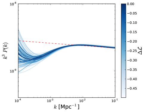
Figure 4: Similar to Figure 3 but for the dimensionless scalar power spectrum. The range in $k$ is cutoff on the largest scales with respect to Figure 3 since the first order slow-roll approximation becomes inaccurate for the the trajectories with the largest $\epsilon$ (smallest $k^{3}P(k)$). The suppression of power driven by the Planck vs Bicep2 tension is clearly seen when compared to a reference power law model (dashed/red line) with $n_{s}=0.962$.

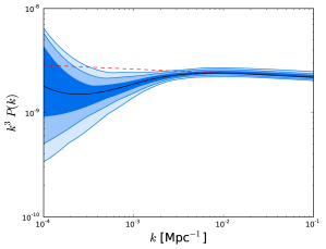
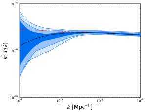
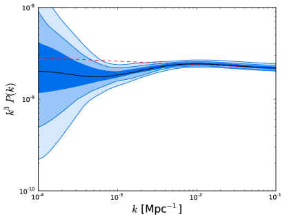
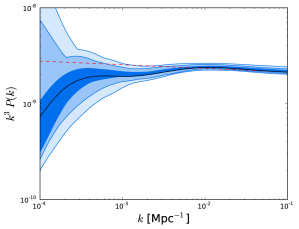
Figure 5: Confidence levels showing $\Delta{\cal L}=-0.5$, -2.0, and -4.5 for (from top-left, clockwise): The $N_{\rm sp}=5$ run, the $N_{\rm sp}=5$ with no Bicep2 included, the $N_{\rm sp}=6$, and $N_{\rm sp}=7$ runs. In each case the red (dashed) line is a reference power law with $n_{s}=0.962$. The 3-$\sigma$ contours encompass the power law over all scales only in the no Bicep2 case. The $N_{\rm sp}=7$ case is only mildly incompatible with the power law case but this model is not favoured by the data.

The significance of the feature, as imprinted on the scalar power spectrum, can be seen in Figure 4 which shows the scalar spectrum, as a function of $k$, for the same set of trajectories. The ensemble is compared to a reference power law model that is compatible with the small scale regime around the pivot scale $k_{\star}=0.05$ Mpc^-1. The reference power law has a spectral index $n_{s}=0.959$ compatible with the peak in the posterior for $n_{s}$ in the run.

The validity of the first order slow-roll assumption used in (2) is limited when $\epsilon\sim 0.1$ for some of the trajectories close to the lower $e$-fold bound. We therefore restrict the $k$ range to smaller scales when looking at the resulting spectra. In the region of the feature of interest $k\sim 10^{-3}$ Mpc^-1 the value of epsilon converges to ${\cal O}(10^{-2})$ which leads to a few percent accuracy in the spectra and other observables.

To assess the stability of the suppression feature seen in the scalar power spectrum we compare similar ensembles for the three different $\epsilon$ runs in Figure 5. The shadings indicate the maximum and minimum bounds covered by ensembles of trajectories that have $\Delta{\cal L}=-0.5$, -2.0, and -4.5 i.e. equivalent to 1, 2, and 3-$\sigma$ thresholds for a Gaussian likelihood. The no Bicep2 case is also shown for the $N_{\rm sp}=5$ case showing that the reference power law model is compatible with the indicative 2-$\sigma$ region. For both favoured models with $N_{\rm sp}=5$ and 6 the power law model is outside of the 3-$\sigma$ region around the scales where the power is suppressed. In the less favoured $N_{\rm sp}=7$ case the power law lies just outside the 3-$\sigma$ region for a very limited range in scales. The analysis indicates that the feature is significant for the most favoured models, or alternatively that the power law hypothesis can be ruled out.

In both the $N_{\rm sp}=5$ and $N_{\rm sp}=6$ models favoured by the data the best-fitting power spectra and distribution around it indicate that the power either levels off or grows in amplitude going to larger scales, $k<5\times 10^{-4}$. This is in agreement with the analysis of Contaldi where a mild, step-like suppression was found to be preferred by the data significantly as opposed to a sharp cutoff due to a fast-roll to slow-roll transition cutoff . In terms of the acceleration, this indicates that the period of inflation extended to earlier times with $\epsilon$ remaining less than unity rather than the feature being due to the start of inflation being just outside the observational window.

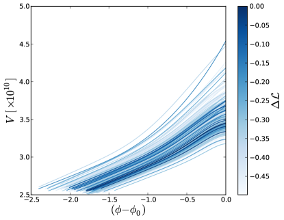
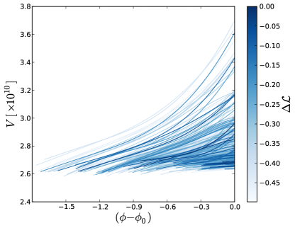
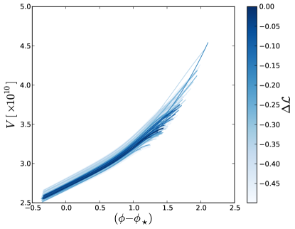
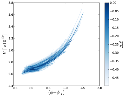
Figure 6: The inflaton potentials $V(\phi)$ corresponding to the “1-$\sigma$” $N_{\rm sp}=5$ ensemble shown in Figure 3. Left: Including the Bicep2 data and Right: excluding the Bicep2 data. In both cases the bottom plot shows the potentials re-centred around the value of $\phi$ at which the pivot scale $k=0.05$ Mpc^-1 is exiting the horizon. The origin of the suppression in scalar power is the mild, transient steepening of the potential around $(\phi-\phi_{0})\sim 0.4$.

IV.3 Inflaton potential

Each of the splined $\epsilon$ trajectories can be related to a scalar potential $V(\phi)$ using (8) and (9). This assumes that inflation is driven by a single scalar with $\phi$ evolving monotonically in time. The relation does not depend on any slow-roll assumption explicitly but there is an implicit dependence on the first order assumption made in relating $\epsilon(N)$ to the primordial power spectra in order to compare with the data.

Figure 6 shows the ensemble of potentials for the 1-$\sigma$ range of $\epsilon$ trajectories in the $N_{\rm sp}=5$ run for the case with and without Bicep2 respectively. The potentials are plotted against the value of $\phi$ centred on $\phi_{0}$ - the value of $\phi$ when the largest mode is exiting the horizon, and also centred on $\phi_{\star}$ - the value of $\phi$ when the pivot scale is exiting the horizon. The latter shows how the Bicep2 data leads to a tightly constrained normalisation and shape of the potential in the region around the pivot scale. The former shows more clearly the shapes of each trajectory.

The origin of the suppression feature can be seen in the potential shapes constrained by Bicep2 as a mild, transient steepening in most of the best-fitting potentials in the initial stages as the field rolls down hill. In this transient region the field velocity increases temporarily which results in an enhanced value of $\epsilon$ and suppressed scalar power. The tensor spectrum is mostly unaffected as it only depends on the integral of $\epsilon$. The total field displacement is also tightly constrained when including Bicep2 since the overall gradients of the curves are similar. This is in contrast to the no Bicep2 case where a much greater range in gradients and curvature of the potential is allowed resulting in very different overall displacements in $\phi$ required to cover the observable window.

V Discussion

We have introduced a method for obtaining posterior distributions in parameters describing the acceleration of the background during inflation. The posteriors are obtained by MCMC exploration of a data likelihood. The method successfully fits the data and the parametrisation is favoured by the Planck+WP+Bicep2 combination of CMB data over traditional power law parametrisation of the primordial spectra.

The method can also be considered as a procedure for the reconstruction of the primordial spectra as we have shown by obtaining derived distributions in $P_{s}(k)$. The tensor mode spectrum can also be obtained but we have omitted it here as it does not show any surprising feature. In the scalar case we have shown that the well known suppression feature driven by the Bicep2 vs Planck tension is also present in this reconstruction and appears to be significant. It is difficult to quantify the significance precisely without comparing to a full distribution of allowed power law models but, from our analysis, it is clear that the power law model is incompatible at least at the 95% confidence level - if not higher.

As a reconstruction method, our procedure can be compared with other non-parametric methods such as those used in Section 7 of planck_inf . One advantage of the parametrised acceleration method used here is that it imposes a physically justified smoothness constraint on the spectrum. This is due to the monotonicity of $H$ and the requirement that $\epsilon<1$ and avoids the problem of over-fitting of the noise in the data which is evident in the structure obtained in direct reconstruction methods.

The method can also be used to reconstruct the form of the inflaton potential $V(\phi)$ under the specific assumptions that there is a single inflaton driving the acceleration. In this case too, we have shown how to obtain a posterior distribution in the possible shape of the potential under these assumptions. The feature seen in the scalar power spectrum is also present in the form of a subtle transient in the gradient of the best-fitting potentials in the relevant range in $\phi$. This method can also be compared to reconstruction methods that either parametrise the potential as a Taylor series around a pivot point (see for example Section 6 of planck_inf ) or Hamilton-Jacobi methods (see for example contaldi_planck ).

If the Bicep2 result is confirmed by further observations it will motivate the careful study of polarisation on large scales. This will allow us to obtain as much information as we can from the tensor modes and methods such as the one used here will be important tools in the quest to understand what the data says about the theory of inflation. Further improvements in the method itself are also possible. A more sophisticated parametrisation of the acceleration that results in less correlated variables should be developed. The function $\epsilon(N)$ could also be expanded on a basis that has better analytic properties than a cubic spline. This would be crucial in order to extend the method to higher orders in slow-roll or to employ exact solutions for the perturbations. This work is left for future studies.

- (1) P. A. RAde et al. [ Bicep2 Collaboration], arXiv:1403.3985 [astro-ph.CO].
- (2) C. R. Contaldi, M. Peloso and L. Sorbo, JCAP 1407, 014 (2014) [arXiv:1403.4596 [astro-ph.CO]].
- (3) R. Flauger, J. C. Hill and D. N. Spergel, arXiv:1405.7351 [astro-ph.CO].
- (4) M. J. Mortonson and U. Seljak, arXiv:1405.5857 [astro-ph.CO].
- (5) L. P. Grishchuk, Sov. Phys. JETP 40, 409 (1975) [Zh. Eksp. Teor. Fiz. 67, 825 (1974)].
- (6) A. A. Starobinsky, JETP Lett. 30, 682 (1979) [Pisma Zh. Eksp. Teor. Fiz. 30, 719 (1979)].
- (7) V. A. Rubakov, M. V. Sazhin and A. V. Veryaskin, Phys. Lett. B 115, 189 (1982).
- (8) R. Fabbri and M. d. Pollock, Phys. Lett. B 125, 445 (1983).
- (9) L. F. Abbott and M. B. Wise, Nucl. Phys. B 244, 541 (1984).
- (10) A. D. Linde, Phys. Lett. B 129, 177 (1983).
- (11) K. Freese, J. A. Frieman and A. V. Olinto, Phys. Rev. Lett. 65, 3233 (1990).
- (12) C. L. Bennett et al. [WMAP Collaboration], Astrophys. J. Suppl. 208, 20 (2013) [arXiv:1212.5225 [astro-ph.CO]].
- (13) P. A. R. Ade et al. [Planck Collaboration], arXiv:1303.5075 [astro-ph.CO].
- (14) K. M. Smith, C. Dvorkin, L. Boyle, N. Turok, M. Halpern, G. Hinshaw and B. Gold, arXiv:1404.0373 [astro-ph.CO].
- (15) A. A. Starobinsky, JETP Lett. 55, 489 (1992) [Pisma Zh. Eksp. Teor. Fiz. 55, 477 (1992)].
- (16) L. Barranco, L. Boubekeur and O. Mena, arXiv:1405.7188 [astro-ph.CO].
- (17) P. A. R. Ade et al. [Planck Collaboration], arXiv:1303.5076 [astro-ph.CO].
- (18) E. D. Stewart and D. H. Lyth, Phys. Lett. B 302, 171 (1993) [gr-qc/9302019].
- (19) Press, W. H., Teukolsky, S. A., Vetterling, W. T., & Flannery, B. P. 1992, Cambridge: University Press, —c1992, 2nd ed.
- (20) A. Lewis and S. Bridle, Phys. Rev. D 66, 103511 (2002) [astro-ph/0205436].
- (21) A. Lewis, A. Challinor and A. Lasenby, Astrophys. J. 538, 473 (2000) [astro-ph/9911177].
- (22) Akaike, H. 1974, IEEE Transactions on Automatic Control, 19, 716
- (23) C. R. Contaldi, M. Peloso, L. Kofman and A. D. Linde, JCAP 0307, 002 (2003) [astro-ph/0303636].
- (24) Planck Collaboration, Ade, P. A. R., Aghanim, N., et al. 2013, arXiv:1303.5082
- (25) C. R. Contaldi and J. S. Horner, arXiv:1312.6067 [astro-ph.CO].