Multistep stochastic mirror descent for risk-averse convex stochastic programs based on extended polyhedral risk measures

Abstract

We consider risk-averse convex stochastic programs expressed in terms of extended polyhedral risk measures. We derive computable confidence intervals on the optimal value of such stochastic programs using the Robust Stochastic Approximation and the Stochastic Mirror Descent (SMD) algorithms. When the objective functions are uniformly convex, we also propose a multistep extension of the Stochastic Mirror Descent algorithm and obtain confidence intervals on both the optimal values and optimal solutions. Numerical simulations show that our confidence intervals are much less conservative and are quicker to compute than previously obtained confidence intervals for SMD and that the multistep Stochastic Mirror Descent algorithm can obtain a good approximate solution much quicker than its nonmultistep counterpart.

Keywords:  Stochastic Optimization, Risk measures, Multistep Stochastic Mirror Descent, Robust Stochastic Approximation.

AMS subject classifications: 90C15, 90C90.

1 Introduction

Consider the convex stochastic optimization problem

$$\left\{\begin{array}[]{l}\min\;f(x):=\mathcal{R}\left[g(x,\xi)\right],\\ x\in X,\end{array}\right.$$ (1.1)

where $\xi\in L_{p}(\Omega,\mathcal{F},\mathbb{P};\mathbb{R}^{s})$ is a random vector with support $\Xi$ and with

• $g:E\times\mathbb{R}^{s}\rightarrow\mathbb{R}$ a Borel function which is convex in $x$ for every $\xi$ and $\mathbb{P}$-summable in $\xi$ for every $x$;

• $X$ a closed and bounded convex set in a Euclidean space $E$; and

• $\mathcal{R}$ an extended polyhedral risk measure [12].

Given a sample $\xi_{1},\ldots,\xi_{N}$ from the distribution of $\xi$, our goal is to obtain online nonasymptotic computable confidence intervals for the optimal value of (1.1) using as estimators of the optimal value variants of the Stochastic Mirror Descent (SMD) algorithm. By computable confidence interval, we mean a confidence interval that does not depend on unknown quantities. For instance, the confidence intervals from [21] and [13] are obtained using SMD and a variant of SMD but are not computable since they require the evaluation of the objective function $f$ at the approximate solution and typically for problems of form (1.1) this evaluation cannot be performed exactly. The terminology online, taken from [18], refers to the fact that the confidence intervals are computed in terms of the sample $\xi^{N}=(\xi_{1},\ldots,\xi_{N})$ used to solve problem (1.1), whereas offline confidence intervals use an additional sample $\xi^{\tilde{N}}=(\xi_{N+1},\ldots,\xi_{N+\tilde{N}})$ independent on $\xi^{N}$. Contrary to asymptotic confidence intervals that are valid as the sample size tends to infinity, nonasymptotic confidence bounds use probability inequalities that are valid for all sample sizes, but they can be more conservative for this reason.

Before deriving a confidence interval on the optimal value of stochastic program (1.1), we need to define an estimator of this optimal value. A natural estimator is the empirical estimator which is obtained replacing the risk measure in the objective function by its empirical estimation. In the case of risk-neutral convex problems (when $\mathcal{R}=\mathbb{E}$ is the expectation), asymptotic and consistency properties of this estimator have been studied extensively. The asymptotic distribution of the empirical estimator is obtained using the Delta method (see [31], [37]) and the Functional Central Limit Theorem. This distribution and the consistency of the estimator were derived in [6], [34], [35] [15], [23], [2], [3], [4]. In [19] the confidence intervals are built using a multiple replication procedure while a single replication is used in [2]. The paper [5] deals more specifically with the computation of asymptotic confidence intervals for the optimal value of risk-neutral multistage stochastic programs. These results were extended to some stochastic programs with integer recourse in [17] and [8].

Less papers have focused on the determination of nonasymptotic confidence intervals on the optimal value of a stochastic convex program. This problem was however studied in [24] for risk-neutral convex problems using Talagrand inequality ([38], [39]). Similar results, using large-deviation type results are obtained in [36] and in [16], [17] for integer models. Instead of using the empirical estimator, the optimal value of (1.1) can be estimated using algorithms for stochastic convex optimization such as the Stochastic Approximation (SA) [29], the Robust Stochastic Approximation (RSA) [26], [27], or the Stochastic Mirror Descent (SMD) algorithm [21]. This approach is used in [21] and [18] where nonasymptotic confidence intervals on the optimal value of a stochastic convex program are derived.

The SMD algorithm applied to stochastic programs minimizing the Conditional Value-at-Risk (CVaR, introduced in [30]) of a cost function was studied in [18]. However, we are not aware of papers deriving confidence intervals for the optimal values of stochastic risk-averse convex programs expressed in terms of large classes of risk measures, namely law invariant coherent or extended polyhedral risk measures (EPRM).

In this context, the contributions of this paper are the following:

• the description and convergence analysis of Stochastic Mirror Descent is based on three important assumptions: (i) convexity of the objective function, (ii) a stochastic oracle provides stochastic subgradients, and (iii) bounds on some exponential moments are available. We extend the SMD algorithm to solve risk-averse stochastic programs that minimize an EPRM of the cost. We provide conditions on these risk measures such that the aforementioned conditions (i), (ii), and (iii) hold and give a formula for stochastic subgradients of the objective function in this situation. Examples of EPRM satisfying these conditions are the expectation, the CVaR, some spectral risk measures, the optimized certainty equivalent, the expected utility with piecewise affine utility function, and any linear combination of these. We also observe that such stochastic programs can be reformulated as risk-neutral stochastic programs with additional variables and constraints, making the SMD for risk-neutral problems directly applicable to these reformulations.

• We provide conditions ensuring that assumptions (i), (ii), and (iii) are satisfied for two-stage stochastic risk-neutral programs and give again formulas for stochastic subgradients of the objective function in this case.

• We define a new computable nonasymptotic online confidence interval on the optimal value of a risk-neutral stochastic convex program using SMD. Numerical simulations show that this confidence interval is much less conservative than the online confidence interval from [18] and is more quickly computed.

• We apply the ideas of the multistep method of dual averaging described in [13] to propose a multistep Stochastic Mirror Descent algorithm. We also analyse the convergence of this variant of SMD and provide computable confidence intervals on the optimal value using this algorithm (contrary to [13] where for the stochastic method of dual averaging the confidence intervals were not computable). We present the results of numerical simulations showing the interest of the multistep variant of SMD on two stochastic (uniformly) convex optimization problems.

• We study the convergence of SMD when the objective function is uniformly convex.

More precisely, the outline of the study is as follows. In Section 2, we introduce (in Subsection 2.1) the assumptions on the class of problems (1.1) considered. In this section we also provide examples of two important classes of problems satisfying these assumptions: two-stage risk-neutral stochastic convex programs (Subsection 2.2) and some risk-averse stochastic convex programs expressed in terms of EPRM (Subsection 2.3). Since problem (1.1) can be expressed, eventually after some reformulation (see Section 2), as a risk-neutral stochastic convex program, we then explain in Sections 3 and 4 how to obtain a nonasymptotic confidence interval for the optimal value of (1.1) in the case when $\mathcal{R}=\mathbb{E}$ is the expectation. Various algorithms are considered. In Section 3, we consider the RSA algorithm (Subsection 3.1) and the SMD algorithm (Subsection 3.2). In each case, on the basis of an independent sample $(\xi_{1},\ldots,\xi_{N})$ of $\xi$, the algorithm produces an approximate optimal value $g^{N}$ for (1.1) and a confidence interval for that optimal value. In the particular case when the objective function $f$ is uniformly convex, we additionally provide confidence intervals for the optimal solution of (1.1). Applying the techniques discussed in [13] to the SMD algorithm, multistep versions of the Stochastic Mirror Descent algorithm are proposed and studied in Section 4 in the case when $f$ is uniformly convex. Confidence intervals for the optimal value of (1.1) obtained using these multistep algorithms are also given. In Section 5 numerical simulations illustrate our results: we show that our confidence intervals are less conservative than previously obtained confidence intervals for SMD and we show the interest of the multistep variant of SMD over its traditional, nonmultistep, implementation. Finally, in Section 6, we comment on future directions of research.

We use the following notation. For a vector $x\in\mathbb{R}^{n}$, $x^{+}$ is the vector with $i$-th component given by $x^{+}(i)=\max(x(i),0)$. We denote by $f^{\prime}(x)$ one of the subgradient(s) of convex function $f$ at $x$. For a norm $\|\cdot\|$ of a Euclidean space $E$ associated to a scalar product $\langle\cdot,\cdot\rangle$, the norm $\|\cdot\|_{*}$ conjugate to $\|\cdot\|$ is given by

$$\|y\|_{*}=\max_{x:\|x\|\leq 1}\,\langle x,y\rangle.$$

We denote the $\ell_{p}$ norm of a vector $x$ in $\mathbb{R}^{n}$ by $\|x\|_{p}$. The closed ball of center $x_{0}$ and radius $R$ is denoted by $B(x_{0},R)$. By $\Pi_{Y}$, we denote the metric projection operator onto the set $Y$, i.e., $\Pi_{Y}(x)=\mbox{arg min}_{y\in Y}\;\|y-x\|_{2}$. For a nonempty set $X\subseteq\mathbb{R}^{n}$, the polar cone $X^{*}$ is defined by $X^{*}=\{x^{*}:\left\langle x,x^{*}\right\rangle\leq 0,\;\forall x\in X\}$, where $\left\langle\cdot,\cdot\right\rangle$ is the standard scalar product on $\mathbb{R}^{n}$. By $\xi^{t}=(\xi_{1},\ldots,\xi_{t})$, we denote the history of the process $(\xi_{t})$ up to time $t$ and by $\mathcal{F}_{t}$ the sigma-algebra generated by $\xi^{t}$. We will denote the Hessian matrix of $f$ at $x$ by $f^{\prime\prime}(x)$. Finally, unless stated otherwise, all relations between random variables are supposed to hold almost surely.

2 Class of problems considered and assumptions

Consider problem (1.1) with $\mathcal{R}$ an EPRM:

Definition 2.1.

[12] Let $(\Omega,\mathcal{F},\mathbb{P})$ be a probability space and let $K(z)=(K_{1}(z),\ldots$, $K_{n_{2,2}}(z))^{\scriptscriptstyle\top}$ for given functions $K_{1},\ldots,K_{n_{2,2}}:\mathbb{R}\rightarrow\mathbb{R}$. A risk measure $\mathcal{R}$ on $L_{p}(\Omega,\mathcal{F},\mathbb{P})$ with $p\in[2,\infty)$ is called extended polyhedral if there exist matrices $A_{1},A_{2},B_{2,0},B_{2,1}$, and vectors $a_{1},a_{2},c_{1},c_{2}$ such that for every random variable $Z\in L_{p}(\Omega,\mathcal{F},\mathbb{P})$

$$\mathcal{R}(Z)=\left\{\begin{array}[]{l}\displaystyle{\inf}\;c_{1}^{\scriptscriptstyle\top}y_{1}+\mathbb{E}[c_{2}^{\scriptscriptstyle\top}y_{2}]\\ y_{1}\in\mathbb{R}^{k_{1}},\;y_{2}\in L_{p}(\Omega,\mathcal{F},\mathbb{P};\mathbb{R}^{k_{2}}),\\ A_{1}y_{1}\leq a_{1},\;A_{2}y_{2}\leq a_{2}\;a.s.,\\ B_{2,1}y_{1}+B_{2,0}y_{2}=K(Z)\;a.s.\end{array}\right.$$ (2.2)

In what follows, we make the following assumption on $K$ in (2.2):

• The function $K(z)$ is affine: $K(z)=zk_{2}+{\tilde{k}}_{2}$ for some vectors $k_{2},{\tilde{k}}_{2}$.

Representation (2.2) can alternatively be written

$$\mathcal{R}(Z)=\left\{\begin{array}[]{l}\displaystyle{\inf}_{y_{1}}\;c_{1}^{\scriptscriptstyle\top}y_{1}+\mathbb{E}[\mathcal{Q}(y_{1},Z)]\\ A_{1}y_{1}\leq a_{1},\end{array}\right.$$ (2.3)

where the recourse function $\mathcal{Q}(y_{1},z)$ is given by

$$\mathcal{Q}(y_{1},z)=\left\{\begin{array}[]{l}\displaystyle{\inf}_{y_{2}}\;c_{2}^{\scriptscriptstyle\top}y_{2}\\ A_{2}y_{2}\leq a_{2}\\ B_{2,0}y_{2}=zk_{2}+{\tilde{k}}_{2}-B_{2,1}y_{1}.\end{array}\right.$$ (2.4)

In other words, $\mathcal{R}(Z)$ is the optimal value of a two-stage stochastic program where $Z$ appears in the right-hand side of the second-stage problem. It follows that we can re-write (1.1) as

$$\left\{\begin{array}[]{l}\displaystyle{\inf_{y_{1},x}}\;c_{1}^{\scriptscriptstyle\top}y_{1}+\mathbb{E}\Big{[}\mathcal{Q}\Big{(}y_{1},g(x,\xi)\Big{)}\Big{]}\\ A_{1}y_{1}\leq a_{1},\;x\in X,\end{array}\right.$$ (2.5)

with $\mathcal{Q}(\cdot,\cdot)$ given by (2.4). This problem is of the form (1.1) with $\mathcal{R}$ the expectation and with $x,g(x,\xi)$, and $X$ respectively replaced by ${\tilde{x}}=(y_{1},x)$, ${\tilde{g}}({\tilde{x}},\xi)=c_{1}^{\scriptscriptstyle\top}y_{1}+\mathcal{Q}\Big{(}y_{1},g(x,\xi)\Big{)}$, and ${\tilde{X}}=\{{\tilde{x}}=(y_{1},x):x\in X,A_{1}y_{1}\leq a_{1}\}$.

For this reason, in Sections 3 and 4, we focus on risk-neutral stochastic problems of the form

$$\left\{\begin{array}[]{l}\min\;f(x):=\mathbb{E}\left[g(x,\xi)\right],\\ x\in X.\end{array}\right.$$ (2.6)

However, our analysis is based on some assumptions on $f,X$, and $\xi$, to be described in the next section. When reformulating risk-averse problem (1.1) under the form (2.6), introducing additional variables and constraints, one has to make some assumptions on the problem structure and on the EPRM in such a way that this reformulation (2.6) of the problem satisfies our assumptions. This issue is addressed in Subsection 2.3.

2.1 Assumptions

For problem (2.6), in addition to the assumptions on $f$ and $X$ mentioned in the introduction, we make the following assumptions:

Assumption 1. All subgradients of the objective function are bounded on $X$:

$$\mbox{there exists }0\leq L<+\infty\mbox{ such that }\|f^{\prime}(x)\|_{*}\leq L\mbox{ for every }x\in X.$$

Note that Assumption 1 holds if $f$ is finite in a neighborhood of $X$.

Stochastic Oracle. We assume that samples of $\xi$ can be generated and the existence of a stochastic oracle: at $t$-th call to the oracle, $x\in X$ being the query point, the oracle returns $g(x,\xi_{t})\in\mathbb{R}$ and a measurable selection $G(x,\xi_{t})$ of a stochastic subgradient $G(x,\xi_{t})\in\partial_{x}g(x,\xi_{t})$, where $\xi_{1},\xi_{2},...$ is an i.i.d sample of $\xi$. We treat $g(x,\xi)$ as an estimate of $f(x)$ and $G(x,\xi)$ as an estimate of a subgradient of $f$ at $x$.

Assumption 2. Our estimates are unbiased:

$$\forall x\in X:f(x)={\mathbb{E}}_{\xi}\left[g(x,\xi)\right]\ \;\mbox{ and }\;\ f^{\prime}(x):={\mathbb{E}}_{\xi}\left[G(x,\xi)\right]\in\partial f(x).$$

From now on, we set

$$\delta(x,\xi)=g(x,\xi)-f(x),\,\,\Delta(x,\xi)=G(x,\xi)-f^{\prime}(x),$$ (2.7)

so that

$${\mathbb{E}}_{\xi}\left[\delta(x,\xi)\right]=0,\,\,{\mathbb{E}}_{\xi}\left[\Delta(x,\xi)\right]=0.$$

In the sequel, we assume that the observation errors of our oracle satisfy some assumptions (introduced in [21]) additional to having zero means. Specifically, our minimal assumption is the following:

Assumption 3. For some $M_{1},M_{2}\in(0,\infty)$ and for all $x\in X$

$$\begin{array}[]{lrcl}(a)&{\mathbb{E}}\Big{[}\delta^{2}(x,\xi)\Big{]}&\leq&M_{1}^{2},\vspace*{0.1cm}\\ (b)&{\mathbb{E}}\Big{[}\|\Delta(x,\xi)\|_{*}^{2}\Big{]}&\leq&M_{2}^{2}.\end{array}$$ (2.8)

Under our minimal assumption, we will obtain an upper bound on the average error on the optimal value of (1.1). To obtain a confidence interval on this optimal value, we will need a stronger assumption:

Assumption 4. For some $M_{1},M_{2}\in(0,\infty)$ and for all $x\in X$ it holds that

$$\begin{array}[]{lrcl}(a)&{\mathbb{E}}\Big{[}\exp\{\delta^{2}(x,\xi)/M_{1}^{2}\}\Big{]}&\leq&\exp\{1\},\vspace*{0.1cm}\\ (b)&{\mathbb{E}}\Big{[}\exp\{\|\Delta(x,\xi)\|_{*}^{2}/M_{2}^{2}\}\Big{]}&\leq&\exp\{1\}.\\ \end{array}$$ (2.9)

Note that condition (2.9) is indeed stronger than condition (2.8): if a random variable $Y$ satisfies $\mathbb{E}\Big{[}\exp\{Y\}\Big{]}\leq\exp\{1\}$ then by Jensen inequality, using the concavity of the logarithmic function, $\mathbb{E}\Big{[}Y\Big{]}=\mathbb{E}\Big{[}\ln\Big{(}\exp\{Y\}\Big{)}\Big{]}\leq\ln\Big{(}\mathbb{E}\Big{[}\exp\{Y\}\Big{]}\Big{)}\leq 1$.

For a given confidence level, a smaller confidence interval can be obtained under an even stronger assumption:

Assumption 5. For some $M_{1},M_{2}\in(0,\infty)$ and for all $x\in X$ it holds that

$$\begin{array}[]{lrcl}(a)&{\mathbb{E}}\Big{[}\exp\{\delta^{2}(x,\xi)/M_{1}^{2}\}\Big{]}&\leq&\exp\{1\},\vspace*{0.1cm}\\ (b)&\|\Delta(x,\xi)\|_{*}&\leq&M_{2}\mbox{\ almost surely}.\end{array}$$ (2.10)

Observe that the validity of (2.10) for all $x\in X$ and some $M_{1},M_{2}$ implies the validity of (2.9) for all $x\in X$ with the same $M_{1},M_{2}$.

The computation of the confidence intervals on the optimal value of (1.1) using the SMD and multistep SMD algorithms presented in Sections 3 and 4 requires the knowledge of constants $L,M_{1}$, and $M_{2}$ satisfying the assumptions above. For instance, the best (smallest) constants $M_{1},M_{2}$ satisfying Assumption 4 are $M_{1}=\sup_{x\in X}\pi[\delta(x,\cdot)]$ and $M_{2}=\sup_{x\in X}\pi[\|\Delta(x,\cdot)\|_{*}]$ where $\pi$ is the Orlicz semi-norm given by

$$\pi[h]=\inf\big{\{}M\geq 0:\;\mathbb{E}\{\exp\{h^{2}(\xi)/M^{2}\}\}\leq\exp\{1\}\big{\}}.$$

For many problems of form (1.1) with $\mathcal{R}=\mathbb{E}$ the expectation operator, upper bounds on these best constants can be computed analytically, see for instance [21], [18], [11].

2.2 Two-stage stochastic convex programs

Consider the case when (1.1) is a two-stage risk-neutral stochastic convex program, i.e., $\mathcal{R}=\mathbb{E}$ is the expectation, $x$ is the first-stage decision variable, $f(x)=f_{1}(x)+\mathbb{E}_{\xi}[\mathcal{Q}(x,\xi)]$ where $\mathcal{Q}(x,\xi)$ is the second-stage cost given by

$$\mathcal{Q}(x,\xi)=\left\{\begin{array}[]{l}\min_{y}\;f_{2}(x,y,\xi)\\ y\in\mathcal{S}(x,\xi)=\{y:g_{2}(x,y,\xi)\leq 0,Ax+By=\xi\}\end{array}\right.$$ (2.11)

for some function $g_{2}$ taking values in $\mathbb{R}^{m}$ and some random vector $\xi\in L_{p}(\Omega,\mathcal{F},\mathbb{P})$ with $p\geq 2$ and support $\Xi$. We make the following assumptions:

• $X$ is a nonempty, compact, and convex set;

• $f_{1}$ is convex, proper, lower semicontinuous, and is finite in a neighborhood of $X$;

• for every $x\in X$ and $y\in\mathbb{R}^{q}$ the function $f_{2}(x,y,\cdot)$ is measurable and for every $\xi\in\Xi$, the function $f_{2}(\cdot,\cdot,\xi)$ is differentiable and convex;

• for every $\xi\in\Xi$, the function $g_{2}(\cdot,\cdot,\xi)$ is convex and differentiable;

• for every $x\in X$ and for every $\xi\in\Xi$ the set $\mathcal{S}(x,\xi)$ is compact and there exists $y_{x,\xi}\in\mathcal{S}(x,\xi)$ such that $g_{2}(x,y_{x,\xi},\xi)<0$.

With the notation of Section 1, we have $f(x)=\mathbb{E}[g(x,\xi)]$ where $g(x,\xi)=f_{1}(x)+\mathcal{Q}(x,\xi)$. Assumptions (A1), (A2), and (A3) imply the convexity of $f$. Assumptions (A2) and (A4) imply that for every $\xi\in\Xi$, the second-stage cost $\mathcal{Q}(x,\xi)$ is finite which implies the finiteness of $\delta(x,\xi)$ for every $x\in X$. Relations (2.8)(a), (2.9)(a), and (2.10)(a) in respectively Assumptions 3, 4, and 5 are thus satisfied. Assumptions (A2), (A3), and (A4) imply that for every $\xi\in\Xi$, the function $x\rightarrow\mathcal{Q}(x,\xi)$ is subdifferentiable on $X$ with bounded subgradients at any $x\in X$. For fixed $x\in X$ and $\xi\in\Xi$, let $y(x,\xi)$ be an optimal solution of (2.11) and consider the dual problem

$$\sup_{\lambda\in\mathbb{R}^{s},\mu\geq 0}\;\theta_{x,\xi}(\lambda,\mu)$$ (2.12)

for the dual function

$$\theta_{x,\xi}(\lambda,\mu)=\displaystyle\inf_{y\in\mathbb{R}^{q}}\;f_{2}(x,y,\xi)+\lambda^{\scriptscriptstyle\top}(Ax+By-\xi)+\mu^{\scriptscriptstyle\top}g_{2}(x,y,\xi).$$

Let $(\lambda(x,\xi),\mu(x,\xi))$ be an optimal solution of (2.12) (for problem (2.11), $\lambda(x,\xi)$ and $\mu(x,\xi)$ are optimal Lagrange multipliers for respectively the equality and inequality constraints). Then for any $x\in X$ and $\xi\in\Xi$, denoting by $I(x,y,\xi):=\{i\in\{1,\ldots,m\}:g_{2,i}(x,y,\xi)=0\}$ the set of active inequality constraints at $y$ for problem (2.11),

$$s(x,\xi)=\nabla_{x}f_{2}(x,y(x,\xi),\xi)+A^{\scriptscriptstyle\top}\lambda(x,\xi)+\sum_{i\in I(x,y(x,\xi),\xi)}\mu_{i}(x,\xi)\nabla_{x}g_{2,i}(x,y(x,\xi),\xi)$$

belongs to the subdifferential $\partial_{x}\mathcal{Q}(x,\xi)$ and is bounded (see [10] for instance for a proof). As a result, for any $x\in X$, denoting by $s_{1}(x)$ an arbitrary element from $\partial f_{1}(x)$, $f^{\prime}(x):=\mathbb{E}[G(x,\xi)]$ is a subgradient of $f$ at $x$ for $G(x,\xi)=s_{1}(x)+s(x,\xi)$ and recalling that (A1) holds, $\|G(x,\xi)\|_{*}$ is bounded for any $x\in X$ and $\xi\in\Xi$. It follows that Assumption 1 is satisfied as well as Relations (2.8)(b), (2.9)(b), and (2.10)(b) in respectively Assumptions 3, 4, and 5.

2.3 Risk-averse stochastic convex programs

Consider reformulation (2.5) of problem (1.1). To guarantee the convexity of the objective function in this problem as well as Assumptions 1-5, we make the following assumptions on $\mathcal{R}$ and $g$:

• Complete recourse: $Y_{1}:=\{y_{1}:A_{1}y_{1}\leq a_{1}\}$ is nonempty and bounded and $\{B_{2,0}y_{2}:A_{2}y_{2}\leq a_{2}\}=\mathbb{R}^{n_{2,2}}$.

• The feasible set

  $$\mathcal{D}=\{\lambda=(\lambda_{1},\lambda_{2})\in\mathbb{R}^{n_{2,2}}\small{\times}\mathbb{R}^{n_{2,1}}\;:\;\lambda_{2}\leq 0,\;\;B_{2,0}^{{\scriptscriptstyle\top}}\lambda_{1}+A_{2}^{{\scriptscriptstyle\top}}\lambda_{2}=c_{2}\}$$ (2.13)

  of the dual of the second-stage problem (2.4) is nonempty.

• The set $\mathcal{D}$ given by (2.13) is bounded.

• For the set $\mathcal{D}$ given by (2.13), we have that $\mathcal{D}\subseteq{\{-k_{2}\}}^{*}\small{\times}\mathbb{R}^{n_{2,1}}$.

• For every $\xi\in\Xi$, the function $g(\cdot,\xi)$ is convex and lower semicontinuous on $X$ and finite in a neighborhood of $X$.

If $X$ is closed, bounded, and convex, (A1’) implies that ${\tilde{X}}$ is also closed, bounded and convex. Moreover, we can show that assumptions (A1’), (A2’), (A3’), (A4’), and (A5’) imply that the objective function in (2.5) is convex and has bounded subgradients:

Lemma 2.2.

Consider the objective function $f(\tilde{x})=c_{1}^{\scriptscriptstyle\top}y_{1}+\mathbb{E}\Big{[}\mathcal{Q}\Big{(}y_{1},g(x,\xi)\Big{)}\Big{]}$ of (2.5) in variable ${\tilde{x}}=(y_{1},x)$. Assume that (A1’), (A2’), (A3’), (A4’), and (A5’) hold. Then

• $\mathcal{Q}\Big{(}y_{1},g(x,\tilde{\xi})\Big{)}$ is finite for every $\tilde{\xi}$ and every $\tilde{x}\in\tilde{X}=\{{\tilde{x}}=(y_{1},x):x\in X,A_{1}y_{1}\leq a_{1}\}$;

• for every $\tilde{\xi}\in\Xi$, the function $\tilde{x}\rightarrow{\tilde{\mathcal{Q}}}_{\tilde{\xi}}(\tilde{x})=\mathcal{Q}\Big{(}y_{1},g(x,\tilde{\xi})\Big{)}$ is convex and has bounded subgradients on $\tilde{X}$;

• $f$ is convex and has bounded subgradients on $\tilde{X}$.

Proof.

Since (A1’) holds, for every $y_{1}\in Y_{1}$ and every $z\in\mathbb{R}$, the feasible set of problem (2.4) which defines $\mathcal{Q}(y,z)$ is nonempty. Due to (A2’), the feasible set of the dual of this problem is nonempty too. It follows that both the primal and the dual have the same finite optimal value (this shows item (i)) and by duality we can express $\mathcal{Q}(y_{1},z)$ as the optimal value of the dual problem:

$$\mathcal{Q}(y_{1},z)=\max_{(\lambda_{1},\lambda_{2})\in\mathcal{D}}\lambda_{1}^{\scriptscriptstyle\top}(zk_{2}+{\tilde{k}}_{2}-B_{2,1}y_{1})+\lambda_{2}^{\scriptscriptstyle\top}a_{2}$$ (2.14)

with $\mathcal{D}$ given by (2.13). Next, observe that $\mathcal{Q}(y_{1},\cdot)$ is monotone:

$$\forall y_{1}\in Y_{1},\;\forall z_{1},z_{2}\in\mathbb{R},\;z_{1}\geq z_{2}\Rightarrow\mathcal{Q}(y_{1},z_{1})\geq\mathcal{Q}(y_{1},z_{2}).$$ (2.15)

Indeed, if $z_{1}\geq z_{2}$, for every $(\lambda_{1},\lambda_{2})\in\mathcal{D}$, since (A4’) holds, we have $\lambda_{1}^{\scriptscriptstyle\top}k_{2}\geq 0$ and

$$\lambda_{1}^{\scriptscriptstyle\top}(z_{1}k_{2}+{\tilde{k}}_{2}-B_{2,1}y_{1})+\lambda_{2}^{\scriptscriptstyle\top}a_{2}\geq\lambda_{1}^{\scriptscriptstyle\top}(z_{2}k_{2}+{\tilde{k}}_{2}-B_{2,1}y_{1})+\lambda_{2}^{\scriptscriptstyle\top}a_{2}$$

for every $y_{1}\in Y_{1}$. Taking the maximum when $(\lambda_{1},\lambda_{2})\in\mathcal{D}$ in each side of the previous inequality gives $\mathcal{Q}(y_{1},z_{1})\geq\mathcal{Q}(y_{1},z_{2})$. Now take $\tilde{\xi}$ a realization of $\xi$ and $\tilde{x}=(y_{1},x),{\tilde{x}}_{0}=(y_{1}^{0},x_{0})\in\tilde{X}$. Using the convexity of $g(\cdot,\tilde{\xi})$, we have

$$g(x,\tilde{\xi})\geq g(x_{0},\tilde{\xi})+G(x_{0},\tilde{\xi})^{\scriptscriptstyle\top}(x-x_{0})$$

recalling that $G(x_{0},\xi)$ is a measurable selection of a stochastic subgradient of $g(\cdot,\xi)$ at $x_{0}$. Combining this inequality and (2.15) gives

$${\tilde{\mathcal{Q}}}_{\tilde{\xi}}(\tilde{x})=\mathcal{Q}\Big{(}y_{1},g(x,\tilde{\xi})\Big{)}\geq\mathcal{Q}\Big{(}y_{1},g(x_{0},\tilde{\xi})+G(x_{0},\tilde{\xi})^{\scriptscriptstyle\top}(x-x_{0})\Big{)}$$

for every $y_{1}\in Y_{1}$. Next, we have that $\mathcal{Q}(y_{1},z)$ is convex and its subdifferential is given by

$$\partial\mathcal{Q}(y_{1},z)=\left\{\left(\begin{array}[]{cc}-B_{2,1}^{\scriptscriptstyle\top}\lambda_{1}\\ \lambda_{1}^{\scriptscriptstyle\top}k_{2}\end{array}\right):(\lambda_{1},\lambda_{2})\in\mathcal{D}_{y_{1},z}\right\}$$

where $\mathcal{D}_{y_{1},z}$ is the set of optimal solutions to the dual problem (2.14). Denoting by $(\lambda_{1}(y_{1},z),\lambda_{2}(y_{1},z))$ an optimal solution to (2.14), we then have

$${\tilde{\mathcal{Q}}}_{\tilde{\xi}}(\tilde{x})=\mathcal{Q}\Big{(}y_{1},g(x,\tilde{\xi})\Big{)}\geq{\tilde{\mathcal{Q}}}_{\tilde{\xi}}(\tilde{x}_{0})+\left(\begin{array}[]{c}-B_{2,1}^{\scriptscriptstyle\top}\lambda_{1}(y_{1}^{0},g(x_{0},\tilde{\xi}))\\ \lambda_{1}(y_{1}^{0},g(x_{0},\tilde{\xi}))^{\scriptscriptstyle\top}k_{2}G(x_{0},\tilde{\xi})\end{array}\right)^{\scriptscriptstyle\top}\Big{(}\tilde{x}-\tilde{x}_{0}\Big{)}.$$

It follows that for every $\tilde{\xi}$, ${\tilde{\mathcal{Q}}}_{\tilde{\xi}}(\cdot)$ is convex and its subdifferential is given by

$$\partial{\tilde{\mathcal{Q}}}_{\tilde{\xi}}(y_{1}^{0},x_{0})=\left\{\left(\begin{array}[]{cc}-B_{2,1}^{\scriptscriptstyle\top}\lambda_{1}\\ \lambda_{1}^{\scriptscriptstyle\top}k_{2}G(x_{0},\tilde{\xi})\end{array}\right):(\lambda_{1},\lambda_{2})\in\mathcal{D}_{y_{1}^{0},\,g(x_{0},\tilde{\xi})}\right\}.$$

Since $\mathcal{D}_{y_{1}^{0},\,g(x_{0},\tilde{\xi})}$ is a subset of the bounded set $\mathcal{D}$ and since (A5’) holds, all subgradients of ${\tilde{\mathcal{Q}}}_{\tilde{\xi}}(\cdot)$ are bounded for every $\tilde{\xi}\in\Xi$: we have proved (ii). Item (iii) follows from (ii) and the fact that $f$ is finite in a neighborhood of $\tilde{X}$. $\Box$

It follows from Lemma 2.2-(iii) that Assumption 1 is satisfied. We also have $\delta(\tilde{x},\xi)=\mathcal{Q}_{\xi}(\tilde{x})-\mathbb{E}[\mathcal{Q}_{\xi}(\tilde{x})]$, which is finite for every $\xi$ and $\tilde{x}\in\tilde{X}$ using Lemma 2.2-(i). It follows that relations (2.8)(a), (2.9)(a), and (2.10)(a) in respectively Assumptions 3, 4, and 5 are satisfied. Finally Lemma 2.2-(ii) shows that relations (2.8)(b), (2.9)(b), and (2.10)(b) in respectively Assumptions 3, 4, and 5 are also satisfied. This shows that we can use the developments of Sections 3.1, and 3.2 to solve problem (1.1) and to obtain a confidence interval on its optimal value when $\mathcal{R}$ is an EPRM and when assumptions (A0’), (A1’), (A2’), (A3’), (A4’), and (A5’) are satisfied.

Risk-averse stochastic programs expressed in terms of EPRMs share many properties with risk-neutral stochastic programs. Moreover, many popular risk measures can be written as EPRMs satisfying assumptions (A0’), (A1’), (A2’), (A3’), and (A4’). Examples of such risk measures are the CVaR, some spectral risk measures, the optimized certainty equivalent and the expected utility with piecewise affine utility function. We refer to Examples 2.16 and 2.17 in [12] for a discussion on these examples. Conditions ensuring that an EPRM is convex, coherent or consistent with second order stochastic dominance are given in [12]. Multiperiod versions of these risk measures are also defined in [12]. In this context, a convenient property of the corresponding risk-averse program is that we can write dynamic programming equations and solve it, in the case when the problem is convex, by decomposition using for instance Stochastic Dual Dynamic Programming (SDDP) [22]; see [12] for more details and examples of multiperiod EPRM. EPRM are an extension of the polyhedral risk measures introduced in [7] where the reader will find additional examples of (extended) polyhedral risk measures.

Throughout the paper, we will use two (classes of) problems of form (1.1) for which we will detail the computation of the parameters necessary to obtain the confidence intervals on their optimal value given in Sections 3 and 4, in particular parameters $L,M_{1}$, and $M_{2}$ introduced in Section 2.1. These problems are described in the next section.

2.4 Examples

We provide two classes of problems that will be used to illustrate our results.

1. The first class of problems writes

   $$\left\{\begin{array}[]{l}\min f(x)=\mathbb{E}\Big{[}\alpha_{0}\xi^{\scriptscriptstyle\top}x+{\alpha_{1}\over 2}\left(\left({\xi^{\scriptscriptstyle\top}x}\right)^{2}+\lambda_{0}\|x\|_{2}^{2}\right)\Big{]}\\ x\in X:=\{x\in\mathbb{R}^{n}:\sum_{i=1}^{n}x(i)=a,\;x(i)\geq b,i=1,\ldots,n\},\end{array}\right.$$ (2.16)

   where $n\geq 3$, $\alpha_{1},a>0$, $b,\lambda_{0}\geq 0$, with $b<a/n$, and the support $\Xi$ of $\xi$ is a part of the unit box $\{\xi=[\xi(1);...;\xi(n)]\in\mathbb{R}^{n}:\|\xi\|_{\infty}\leq 1\}$.

   If $a=1$ and $b=0$, taking $\|\cdot\|=\|\cdot\|_{1}$, $\|\cdot\|_{*}=\|\cdot\|_{\infty}$, straightforward computations (see [11]) show that Assumptions 1-5 are satisfied for this problem with $L=|\alpha_{0}|+\alpha_{1}(1+\lambda_{0})$, $M_{1}=2|\alpha_{0}|+0.5\alpha_{1}$, and $M_{2}=2|\alpha_{0}|+\alpha_{1}$.

   If $a=1$ and $b=0$, taking $\|\cdot\|=\|\cdot\|_{2}=\|\cdot\|_{*}$, and $G(x,\xi)=\alpha_{0}\xi+\alpha_{1}(\xi\xi^{\scriptscriptstyle\top}+\lambda_{0}I)x$, we have for every $x\in X$ that

   $$\begin{array}[]{lll}\|G(x,\xi)-\mathbb{E}[G(x,\xi)]\|_{2}&\leq&|\alpha_{0}|\|\xi-\mathbb{E}[\xi]\|_{2}+\alpha_{1}\|(\xi\xi^{\scriptscriptstyle\top}-\mathbb{E}[\xi\xi^{\scriptscriptstyle\top}])x\|_{2}\\ &\leq&2|\alpha_{0}|\sqrt{n}+\alpha_{1}\sqrt{n}\|\xi\xi^{\scriptscriptstyle\top}-\mathbb{E}[\xi\xi^{\scriptscriptstyle\top}]\|_{\infty}\leq 2\sqrt{n}(|\alpha_{0}|+\alpha_{1}),\end{array}$$

   $$\begin{array}[]{lll}\|\mathbb{E}[G(x,\xi)]\|_{2}&\leq&|\alpha_{0}|\|\mathbb{E}[\xi]\|_{2}+\alpha_{1}\sqrt{n}\|\mathbb{E}[\xi\xi^{\scriptscriptstyle\top}]x\|_{\infty}+\alpha_{1}\lambda_{0}\|x\|_{1}\\ &\leq&|\alpha_{0}|\sqrt{n}+\alpha_{1}(\sqrt{n}+\lambda_{0}),\end{array}$$

   and Assumptions 1 and 5 hold with $L=|\alpha_{0}|\sqrt{n}+\alpha_{1}(\sqrt{n}+\lambda_{0})$, $M_{1}=2|\alpha_{0}|+0.5\alpha_{1}$, and $M_{2}=2\sqrt{n}(|\alpha_{0}|+\alpha_{1})$.

2. The second class of problems amounts to minimizing a linear combination of the expectation and the CVaR of some random linear function:

   $$\left\{\begin{array}[]{l}\min f(x)=\alpha_{0}\mathbb{E}[\xi^{\scriptscriptstyle\top}x]+{\alpha_{1}}CVaR_{\varepsilon}(\xi^{\scriptscriptstyle\top}x)\\ \sum_{i=1}^{n}x(i)=1,\;x\geq 0,\end{array}\right.$$ (2.17)

   where $\alpha_{1},\alpha_{0}\geq 0$, $0<\varepsilon<1$, the support $\Xi$ of $\xi$ is a part of the unit box $\{\xi=[\xi(1);...;\xi(n)]\in\mathbb{R}^{n}:\|\xi\|_{\infty}\leq 1\}$, and

   $${\rm CVaR}_{\varepsilon}(\xi^{\scriptscriptstyle\top}x)=\min_{x_{0}\in\mathbb{R}}\,x_{0}+\mathbb{E}\left[\varepsilon^{-1}[\xi^{\scriptscriptstyle\top}x-x_{0}]^{+}\right]$$

   is the Conditional Value-at-Risk of level $0<\varepsilon<1$; see [30]. Observing that $|\xi^{\scriptscriptstyle\top}x|\leq 1$ a.s., problem (2.17) is of form (2.6) with $X=\{x=[x(1);...;x(n);x(n+1)]\in\mathbb{R}^{n+1}:\;|x(n+1)|\leq 1,\,x(1),...,x(n)\geq 0,\,\sum_{i=1}^{n}x(i)=1\}$ and

   $$g(x,\xi)=\alpha_{0}\xi^{\scriptscriptstyle\top}[x(1);...;x(n)]+\alpha_{1}\left(x(n+1)+{1\over\epsilon}[\xi^{\scriptscriptstyle\top}[x(1);...;x(n)]-x(n+1)]^{+}\right).$$

   We will also consider a perturbed version of this problem given by

   $$\left\{\begin{array}[]{l}\min\alpha_{0}\mathbb{E}[\xi^{\scriptscriptstyle\top}x_{1:n}]+{\alpha_{1}}\left(x(n+1)+\mathbb{E}\left[\varepsilon^{-1}[\xi^{\scriptscriptstyle\top}x_{1:n}-x(n+1)]^{+}\right]\right)+\lambda_{0}\|x_{1:n+1}\|_{2}^{2}\\ -1\leq x(n+1)\leq 1,\sum_{i=1}^{n}x(i)=1,\;x(i)\geq 0,i=1,\ldots,n,\end{array}\right.$$ (2.18)

   for $\lambda_{0}>0$ where $x_{1:n}=[x(1);...;x(n)]$. For problem (2.18), taking $\|\cdot\|=\|\cdot\|_{2}=\|\cdot\|_{*}$, Assumptions 1 and 5 are satisfied (see [11]) with $L=\sqrt{\alpha_{1}^{2}(1-\frac{1}{\varepsilon})^{2}+n(\alpha_{0}+\frac{\alpha_{1}}{\varepsilon})^{2}}+2\lambda_{0}$, $M_{1}=2(\alpha_{0}+\frac{\alpha_{1}}{\varepsilon})$, and $M_{2}=\sqrt{\left(\frac{\alpha_{1}}{\varepsilon}\right)^{2}+4n\left(\alpha_{0}+\frac{\alpha_{1}}{\varepsilon}\right)^{2}}$.

Problems (2.16) and (2.18) have a penalty term in the objective to make the objective function strongly convex so that multistep SMD, as described in Section 4, can be applied to these problems.

3 Quality of the solutions using RSA and SMD

We consider the RSA and SMD algorithms to solve problem (2.6).

3.1 Robust Stochastic Approximation algorithm

In this section, we use the scalar product $\langle x,y\rangle=x^{\scriptscriptstyle\top}y$ and the corresponding norm $\|\cdot\|=\|\cdot\|_{2}$ with dual norm $\|\cdot\|_{*}=\|\cdot\|_{2}$, meaning that (2.8), (2.9), and (2.10) hold with $\|\cdot\|_{*}=\|\cdot\|_{2}$. The Robust Stochastic Approximation algorithm solves (2.6) as follows:
 

Algorithm 1: Robust Stochastic Approximation.

Initialization. Take $x_{1}$ in $X$. Fix the number of iterations $N-1$ and positive deterministic stepsizes $\gamma_{1},\ldots,\gamma_{N}$.

Loop. For $t=1,\ldots,N-1$, compute

$$\begin{array}[]{rcl}x_{t+1}&=&\Pi_{X}(x_{t}-\gamma_{t}G(x_{t},\xi_{t})).\end{array}$$ (3.19)

Outputs:

$$\begin{array}[]{l}x^{N}=\displaystyle\frac{1}{\Gamma_{N}}\sum_{\tau=1}^{N}\gamma_{\tau}x_{\tau}\mbox{ and }g^{N}=\displaystyle\frac{1}{\Gamma_{N}}\left[\sum_{\tau=1}^{N}\gamma_{\tau}g(x_{\tau},\xi_{\tau})\right]\mbox{ with }\Gamma_{N}=\displaystyle\sum_{\tau=1}^{N}\gamma_{\tau}.\end{array}$$ (3.20)

 

Note that by convexity of $X$, we have $x^{N}\in X$ and after $N-1$ iterations, $x^{N}$ is an approximate solution of (2.6). The value $f(x^{N})$ is an approximation of the optimal value of (2.6), but it is not computable since $f$ is not known. Denoting by $x_{*}$ an optimal solution of (2.6), we introduce after $N-1$ iterations the computable approximation

$$g^{N}=\frac{1}{\Gamma_{N}}\left[\displaystyle\sum_{\tau=1}^{N}\gamma_{\tau}g(x_{\tau},\xi_{\tau})\right]$$ (3.21)

of the optimal value $f(x_{*})$ of (2.6) obtained using the points generated by the algorithm and information from the stochastic oracle. Our goal is to obtain exponential bounds on large deviations of this estimate $g^{N}$ of $f(x_{*})$ from $f(x_{*})$ itself, i.e., a confidence interval on the optimal value of (2.6) using the information provided by the RSA algorithm along iterations. We need two technical lemmas. The first one gives an $O(1/\sqrt{N})$ upper bound on the first absolute moment of the estimation error (the average distance of $g^{N}$ to $f(x_{*})$):

Lemma 3.1.

Let Assumptions 1, 2, and 3 hold and assume that the number of iterations $N-1$ of the RSA algorithm is fixed in advance with stepsizes given by

$$\gamma_{\tau}=\gamma=\frac{D_{X}}{\sqrt{2(M_{2}^{2}+L^{2})}\sqrt{N}},\;\tau=1,\ldots,N,$$ (3.22)

where

$$D_{X}=\max_{x\in X}\;\|x-x_{1}\|.$$ (3.23)

Let $g^{N}$ be the approximation of $f(x_{*})$ given by (3.21). Then

$$\mathbb{E}\left[\Big{|}g^{N}-f(x_{*})\Big{|}\right]\leq\frac{M_{1}+D_{X}\sqrt{2(M_{2}^{2}+L^{2})}}{\sqrt{N}}.$$ (3.24)

Proof.

Recalling (3.22), $\frac{\gamma_{\tau}}{\Gamma_{N}}=\frac{1}{N}$ and letting

$$f^{N}=\frac{1}{N}\displaystyle\sum_{\tau=1}^{N}f(x_{\tau}),$$ (3.25)

it is known (see [21], Section 2.2) that under our assumptions

$${\mathbb{E}}\left[f(x^{N})-f(x_{*})\right]\leq{\mathbb{E}}\left[f^{N}-f(x_{*})\right]\leq\frac{D_{X}\sqrt{2(M_{2}^{2}+L^{2})}}{\sqrt{N}}.$$ (3.26)

Since the main steps of the proof of (3.26) will be useful for our further developments, we rewrite them here. Setting $A_{\tau}=\frac{1}{2}\|x_{\tau}-x_{*}\|_{2}^{2}$, we can show (see Section 2.1 in [21] for instance) that

$$\sum_{\tau=1}^{N}\;\gamma_{\tau}\langle G(x_{\tau},\xi_{\tau}),x_{\tau}-x_{*}\rangle\leq A_{1}+\frac{1}{2}\sum_{\tau=1}^{N}\;\gamma_{\tau}^{2}\|G(x_{\tau},\xi_{\tau})\|_{*}^{2}.$$ (3.27)

To save notation, let us set

$$\delta_{\tau}=g(x_{\tau},\xi_{\tau})-f(x_{\tau}),\,\Delta_{\tau}=\Delta(x_{\tau},\xi_{\tau}),\mbox{ and }G_{\tau}=G(x_{\tau},\xi_{\tau})=f^{\prime}(x_{\tau})+\Delta_{\tau}.$$ (3.28)

Inequality (3.27) can be rewritten

$$\sum_{\tau=1}^{N}\;\gamma_{\tau}\langle f^{\prime}(x_{\tau}),x_{\tau}-x_{*}\rangle\leq\frac{D_{X}^{2}}{2}+\frac{1}{2}\sum_{\tau=1}^{N}\;\gamma_{\tau}^{2}\|G_{\tau}\|_{*}^{2}+\sum_{\tau=1}^{N}\;\gamma_{\tau}\langle\Delta_{\tau},x_{*}-x_{\tau}\rangle.$$ (3.29)

Taking into account that by convexity of $f$ we have $f(x_{\tau})-f(x_{*})\leq\langle f^{\prime}(x_{\tau}),x_{\tau}-x_{*}\rangle$, we get

$$\begin{array}[]{rcl}f(x^{N})-f(x_{*})&\leq&f^{N}-f(x_{*})=\displaystyle\frac{1}{\Gamma_{N}}\displaystyle\sum_{\tau=1}^{N}\gamma_{\tau}\Big{(}f(x_{\tau})-f(x_{*})\Big{)}\\ &\leq&\displaystyle\frac{1}{\Gamma_{N}}\left[\displaystyle\frac{D_{X}^{2}}{2}+\frac{1}{2}\displaystyle\sum_{\tau=1}^{N}\;\gamma_{\tau}^{2}\|G_{\tau}\|_{*}^{2}+\displaystyle\sum_{\tau=1}^{N}\;\gamma_{\tau}\langle\Delta_{\tau},x_{*}-x_{\tau}\rangle\right]\end{array}$$ (3.30)

where the first inequality is due to the origin of $x^{N}$ and to the convexity of $f$.

Next, note that under Assumptions 1, 2, and 3,

$$\mathbb{E}\Big{[}\|G_{\tau}\|_{*}^{2}\Big{]}=\mathbb{E}\Big{[}\|f^{\prime}(x_{\tau})+\Delta_{\tau}\|_{*}^{2}\Big{]}\leq 2\mathbb{E}\Big{[}\|f^{\prime}(x_{\tau})\|_{*}^{2}+\|\Delta_{\tau}\|_{*}^{2}\Big{]}\leq 2\Big{[}M_{2}^{2}+L^{2}\Big{]}.$$ (3.31)

Passing to expectations in (3.30), and taking into account that the conditional, $\xi^{\tau-1}:=(\xi_{1},...,\xi_{\tau-1})$ being fixed, expectation of $\Delta_{\tau}$ is zero, while $x_{\tau}$ by construction is a deterministic function of $\xi^{\tau-1}$, we get

$${\mathbb{E}}\Big{[}f(x^{N})-f(x_{*})\Big{]} \leq {\mathbb{E}}\Big{[}f^{N}-f(x_{*})\Big{]}\leq{D_{X}^{2}+\displaystyle\sum_{\tau=1}^{N}\gamma_{\tau}^{2}{\mathbb{E}}\left[\|G_{\tau}\|_{*}^{2}\right]\over 2\Gamma_{N}}$$ (3.32)

$$\leq \displaystyle\frac{1}{\Gamma_{N}}\Big{[}\frac{D_{X}^{2}}{2}+(M_{2}^{2}+L^{2})\sum_{\tau=1}^{N}\gamma_{\tau}^{2}\Big{]}.$$

Using stepsizes (3.22), we have $\Gamma_{N}={{D_{X}\sqrt{N}}\over{\sqrt{2(M_{2}^{2}+L^{2})}}}$. Plugging this value of $\Gamma_{N}$ into (3.32), we obtain the announced inequality (3.26).

We now show that

$${\mathbb{E}}\Big{[}\Big{|}g^{N}-f^{N}\Big{|}\Big{]}\leq\frac{M_{1}}{\sqrt{N}}.$$ (3.33)

First, note that

$$g^{N}-f^{N}={1\over N}\displaystyle\sum_{\tau=1}^{N}\delta_{\tau}.$$ (3.34)

By the same argument as above, the conditional, $\xi^{\tau-1}$ being fixed, expectation of $\delta_{\tau}$ is $0$, whence

$${\mathbb{E}}\Big{[}\Big{(}\displaystyle\sum_{\tau=1}^{N}\delta_{\tau}\Big{)}^{2}\Big{]}=\sum_{\tau=1}^{N}{\mathbb{E}}\Big{[}\delta_{\tau}^{2}\Big{]}\leq NM_{1}^{2},$$

where the concluding inequality is due to (2.8)($a$). We conclude that

$${\mathbb{E}}\Big{[}\Big{|}g^{N}-f^{N}\Big{|}\Big{]}\leq{1\over N}\sqrt{{\mathbb{E}}\left[\left(\displaystyle\sum_{\tau=1}^{N}\delta_{\tau}\right)^{2}\right]}\leq{1\over N}\sqrt{NM_{1}^{2}}={M_{1}\over\sqrt{N}},$$

which is the announced inequality (3.33). Next, observe that by convexity of $f$, $f^{N}\geq f(x^{N})$ and since $x^{N}\in X$, we have $f(x^{N})\geq f(x_{*})$, i.e., $f^{N}-f(x_{*})\geq f(x^{N})-f(x_{*})\geq 0$, so that (3.26) and (3.33) imply

$${\mathbb{E}}\Big{[}|g^{N}-f(x_{*})|\Big{]} \leq {\mathbb{E}}\Big{[}|g^{N}-f^{N}|+|f^{N}-f(x_{*})|\Big{]}={\mathbb{E}}\Big{[}|g^{N}-f^{N}|\Big{]}+{\mathbb{E}}\Big{[}f^{N}-f(x_{*})\Big{]}$$

$$\leq \Big{[}M_{1}+D_{X}\sqrt{2(M_{2}^{2}+L^{2})}\Big{]}\frac{1}{\sqrt{N}},$$

which achieves the proof of (3.24). $\Box$

To proceed, we need the following lemma:

Lemma 3.2.

Let $\xi_{1},\ldots,\xi_{N}$ be random vectors and associated sigma algebras $\mathcal{F}_{\tau}=\sigma(\xi_{1},\ldots,\xi_{\tau}),\tau=1,\ldots,N$. Let $\eta_{\tau},\tau=1,\ldots,N$, be a sequence of real-valued random variables with $\eta_{\tau}$ $\mathcal{F}_{\tau}$-measurable. Let ${\mathbb{E}}_{|\tau-1}\left[\cdot\right]$ be the conditional expectation ${\mathbb{E}}\left[\cdot|\xi^{\tau-1}\right]$ where $\xi^{\tau-1}=(\xi_{1},\ldots,\xi_{\tau-1})$. Assume that

$${\mathbb{E}}_{|\tau-1}\Big{[}\eta_{\tau}\Big{]}=0,\;\;{\mathbb{E}}_{|\tau-1}\Big{[}\exp\{\eta_{\tau}^{2}\}\Big{]}\leq\exp\{1\}.$$ (3.35)

Then, for any $\Theta>0$,

$$\begin{array}[]{ll}\mathbb{P}\left(\displaystyle\sum_{\tau=1}^{N}\eta_{\tau}>\Theta\,\sqrt{N}\right)\leq\exp\{-\Theta^{2}/4\}.\end{array}$$ (3.36)

Proof.

See the Appendix. $\Box$

We are now in a position to provide a confidence interval for the optimal value of (2.6) using the RSA algorithm:

Proposition 3.3.

Assume that the number of iterations $N-1$ of the RSA algorithm is fixed in advance with stepsizes given by (3.22). Let $g^{N}$ be the approximation of $f(x_{*})$ given by (3.21). Then

• if Assumptions 1, 2, 3, and 4 hold, for any $\Theta>0$, we have

  $$\mathbb{P}\left(\Big{|}g^{N}-f(x_{*})\Big{|}>\frac{K_{1}(X)+\Theta K_{2}(X)}{\sqrt{N}}\right)\leq 4\exp\{1\}\exp\{-\Theta\}$$ (3.37)

  where the constants $K_{1}(X)$ and $K_{2}(X)$ are given by

  $$K_{1}(X)=\frac{D_{X}(M_{2}^{2}+2L^{2})}{\sqrt{2(M_{2}^{2}+L^{2})}}\mbox{ and }K_{2}(X)=\frac{D_{X}M_{2}^{2}}{\sqrt{2(M_{2}^{2}+L^{2})}}+2D_{X}M_{2}+M_{1},$$

  with $D_{X}$ given by (3.23).

• If Assumptions 1, 2, 3, and 5 hold, (3.37) holds with the right-hand side replaced by $(3+\exp\{1\})\exp\{-\frac{1}{4}\Theta^{2}\}$.

Proof.

To prove (i), we shall first prove that for any $\Theta>0$,

$$\begin{array}[]{l}\mathbb{P}\left(f^{N}-f(x_{*})>\frac{D_{X}}{\sqrt{2(M_{2}^{2}+L^{2})\,N}}\left[M_{2}^{2}+2L^{2}+\Theta\left[M_{2}^{2}+2M_{2}\sqrt{2(M_{2}^{2}+L^{2})}\right]\right]\right)\\ \leq 2\exp\{1\}\exp\{-\Theta\},\end{array}$$ (3.38)

where $f^{N}$ is given by (3.25). Using Assumption 1, we have $\|G_{\tau}\|_{*}^{2}=\|f^{\prime}(x_{\tau})+\Delta_{\tau}\|_{*}^{2}\leq 2(\|f^{\prime}(x_{\tau})\|_{*}^{2}+\|\Delta_{\tau}\|_{*}^{2})\leq 2(L^{2}+\|\Delta_{\tau}\|_{*}^{2})$. Combined with (3.30), this implies that

$$\begin{array}[]{rcl}f^{N}-f(x_{*})&\leq&\displaystyle\frac{1}{\Gamma_{N}}\left[\frac{D_{X}^{2}}{2}+\displaystyle\sum_{\tau=1}^{N}\gamma_{\tau}^{2}\Big{(}L^{2}+\|\Delta_{\tau}\|_{*}^{2}\Big{)}\right]+\frac{1}{\Gamma_{N}}\displaystyle\sum_{\tau=1}^{N}\gamma_{\tau}\langle\Delta_{\tau},x_{*}-x_{\tau}\rangle\vspace*{0.1cm}\\ &\leq&\displaystyle\frac{D_{X}(M_{2}^{2}+2L^{2})}{\sqrt{2(M_{2}^{2}+L^{2})}\sqrt{N}}+\frac{D_{X}M_{2}^{2}}{\sqrt{2(M_{2}^{2}+L^{2})}\sqrt{N}}{\mathcal{A}}+\frac{2D_{X}M_{2}}{N}{\mathcal{B}}\end{array}$$ (3.39)

where

$${\mathcal{A}}={1\over NM_{2}^{2}}\displaystyle\sum_{\tau=1}^{N}\|\Delta_{\tau}\|_{*}^{2}\;\;\mbox{ and }\;\;{\mathcal{B}}={1\over 2D_{X}M_{2}}\displaystyle\sum_{\tau=1}^{N}\langle\Delta_{\tau},x_{*}-x_{\tau}\rangle.$$ (3.40)

Setting $\zeta_{\tau}=\|\Delta_{\tau}\|_{*}^{2}/M_{2}^{2}$ and invoking (2.9)($b$), we get ${\mathbb{E}}\Big{[}\exp\{\zeta_{\tau}\}\Big{]}\leq\exp\{1\}$ for all $\tau\leq N$, whence, due to the convexity of the exponent,

$${\mathbb{E}}\Big{[}\exp\{{\mathcal{A}}\}\Big{]}={\mathbb{E}}\Big{[}\exp\{{1\over N}\sum_{\tau=1}^{N}\zeta_{\tau}\}\Big{]}\leq\frac{1}{N}\sum_{\tau=1}^{N}{\mathbb{E}}\Big{[}\exp\{\zeta_{\tau}\}\Big{]}\leq\exp\{1\}$$

as well. As a result,

$$\forall\,\Theta>0:\mathbb{P}\Big{(}{\mathcal{A}}>\Theta\Big{)}\leq\exp\{-\Theta\}{\mathbb{E}}\Big{[}\exp\left\{{\mathcal{A}}\right\}\Big{]}\leq\exp\{1-\Theta\}.$$ (3.41)

Now let us set $\eta_{\tau}={1\over 2D_{X}M_{2}}\langle\Delta_{\tau},x_{*}-x_{\tau}\rangle$, so that ${\mathcal{B}}=\sum_{\tau=1}^{N}\eta_{\tau}$. Denoting by ${\mathbb{E}}_{|\tau-1}$ the conditional, $\xi^{\tau-1}$ being fixed, expectation, we have

$${\mathbb{E}}_{|\tau-1}\Big{[}\eta_{\tau}\Big{]}=0\ \;\mbox{ and }\;\ {\mathbb{E}}_{|\tau-1}\Big{[}\exp\{\eta_{\tau}^{2}\}\Big{]}\leq\exp\{1\},$$

where the first relation is due to ${\mathbb{E}}_{|\tau-1}\Big{[}\Delta_{\tau}\Big{]}=0$ combined with the fact that $x_{*}-x_{\tau}$ is a deterministic function of $\xi^{\tau-1}$, and the second relation is due to (2.9)($b$) combined with the fact that $\|x_{*}-x_{\tau}\|\leq 2D_{X}$. Using Lemma 3.2, we obtain for any $\Theta>0$

$$\begin{array}[]{ll}\mathbb{P}\Big{(}{\mathcal{B}}>\Theta\,\sqrt{N}\Big{)}\leq\exp\{-\Theta^{2}/4\}.\end{array}$$ (3.42)

Combining (3.39), (3.41), and (3.42), we obtain for every $\Theta>0$

$$\begin{array}[]{l}\mathbb{P}\left(f^{N}-f(x_{*})>\displaystyle\frac{D_{X}(M_{2}^{2}+2L^{2})}{\sqrt{2(M_{2}^{2}+L^{2})\,N}}+\frac{\Theta}{\sqrt{N}}\left[\frac{D_{X}M_{2}^{2}}{\sqrt{2(M_{2}^{2}+L^{2})}}+2D_{X}M_{2}\right]\right)\\ \leq\exp\{1-\Theta\}+\exp\{-\Theta^{2}/4\}\leq 2\exp\{1\}\exp\{-\Theta\},\end{array}$$ (3.43)

which is (3.38).

Next,

$$g^{N}-f^{N}={M_{1}\over N}\left[\sum_{\tau=1}^{N}\chi_{\tau}\right],\,\,\chi_{\tau}={\delta_{\tau}\over M_{1}}.$$

Observing that $\chi_{\tau}$ is a deterministic function of $\xi^{\tau}$ and that

$${\mathbb{E}}_{|\tau-1}\Big{[}\chi_{\tau}\Big{]}=0\ \;\mbox{ and }\;\ {\mathbb{E}}_{|\tau-1}\Big{[}\exp\{\chi_{\tau}^{2}\}\Big{]}\leq\exp\{1\},\,1\leq\tau\leq N$$

(we have used (2.9)($a$)), we can use once again Lemma 3.2 to obtain for all $\Theta>0$:

$$\mathbb{P}\left(g^{N}-f^{N}>\Theta{M_{1}\over\sqrt{N}}\right)\leq\exp\{-\Theta^{2}/4\}$$

and

$$\mathbb{P}\left(g^{N}-f^{N}<-\Theta{M_{1}\over\sqrt{N}}\right)\leq\exp\{-\Theta^{2}/4\}.$$

Thus,

$$\forall\;\Theta>0:\mathbb{P}\left(\Big{|}g^{N}-f^{N}\Big{|}>\Theta{M_{1}\over\sqrt{N}}\right)\leq 2\exp\{-\Theta^{2}/4\},$$

which, combined with (3.38) implies (3.37), i.e., item (i) of the lemma.

Finally, under Assumption 5, we have $\mathbb{P}\Big{(}{\mathcal{A}}>1\Big{)}=0$, which combines with (3.41) to imply that

$$\forall\Theta>0:\mathbb{P}\Big{(}{\mathcal{A}}>\Theta\Big{)}\leq\exp\{1-\Theta^{2}\},$$

meaning that the right-hand side in (3.38) can be replaced with $\exp\{1-\Theta^{2}\}+\exp\{-\Theta^{2}/4\}$, which proves item (ii). $\Box$

Setting

$$a(\Theta,N)=\frac{\Theta M_{1}}{\sqrt{N}}\mbox{ and }b(\Theta,X,N)=\frac{K_{1}(X)+\Theta(K_{2}(X)-M_{1})}{\sqrt{N}},$$ (3.44)

we now combine the upper bound on $f(x_{*})$

$${\tt{Up}}_{1}(\Theta_{1},N)=\frac{1}{N}\sum_{t=1}^{N}g(x_{t},\xi_{t})+a(\Theta_{1},N)=g^{N}+a(\Theta_{1},N),$$ (3.45)

from [18] with the lower bound

$${\tt{Low}}_{1}(\Theta_{2},\Theta_{3},N)=g^{N}-b(\Theta_{2},X,N)-a(\Theta_{3},N),$$ (3.46)

from Proposition 3.3 to obtain a new confidence interval on the optimal value $f(x_{*})$:

Corollary 3.4.

Let ${\tt{Up}}_{1}$ and ${\tt{Low}}_{1}$ be the upper and lower bounds given by respectively (3.45) and (3.46). Then if Assumptions 1, 2, 3, and 5 hold, for any $\Theta_{1},\Theta_{2},\Theta_{3}>0$, we have

$$\mathbb{P}\left(f(x_{*})\in\Big{[}{\tt{Low}}_{1}(\Theta_{2},\Theta_{3},N),{\tt{Up}}_{1}(\Theta_{1},N)\Big{]}\right)\geq 1-e^{-\Theta_{1}^{2}/4}-e^{1-\Theta_{2}^{2}}-e^{-\Theta_{2}^{2}/4}-e^{-\Theta_{3}^{2}/4}.$$ (3.47)

If Assumptions 1, 2, 3, and 4 hold, then (3.47) holds with the term $e^{1-\Theta_{2}^{2}}$ replaced by $e^{1-\Theta_{2}}$.

Proof.

Let Assumptions 1, 2, 3, and 5 hold. Since $f(x_{t})\geq f(x_{*})$ almost surely, using Lemma 3.2 we get

$$\mathbb{P}\Big{(}{\tt{Up}}_{1}(\Theta_{1},N)<f(x_{*})\Big{)}\leq\mathbb{P}\Big{(}\frac{1}{N}\sum_{t=1}^{N}\Big{[}g(x_{t},\xi_{t})-f(x_{t})\Big{]}<-\frac{\Theta_{1}M_{1}}{\sqrt{N}}\Big{)}\leq e^{-\Theta_{1}^{2}/4}.$$

Next, using the proof of Proposition 3.3, we can define sets $S_{1},S_{2}\subset\Omega$ such that under Assumptions 1, 2, 3, and 5 we have $\mathbb{P}(S_{1})\geq 1-e^{1-\Theta_{2}^{2}}-e^{-\Theta_{2}^{2}/4}$ (resp. $\mathbb{P}(S_{2})\geq 1-e^{-\Theta_{3}^{2}/4}$) and on $S_{1}$ (resp. on $S_{2}$) we have $f^{N}-b(\Theta_{2},X,N)\leq f(x_{*})$ (resp. $g^{N}-f^{N}\leq a(\Theta_{3},N)$). Now observe that on $S_{1}\cap S_{2}$ we have $f(x_{*})\geq{\tt{Low}}_{1}(\Theta_{2},\Theta_{3},N)$ which implies that

$$\mathbb{P}(f(x_{*})\geq{\tt{Low}}_{1}(\Theta_{2},\Theta_{3},N))\geq\mathbb{P}(S_{1}\cap S_{2})\geq 1-e^{1-\Theta_{2}^{2}}-e^{-\Theta_{2}^{2}/4}-e^{-\Theta_{3}^{2}/4}$$

and (3.47) follows. $\Box$

Remark 3.5.

Let Assumptions 1, 2, 3, and 5 hold. To equilibrate the risks, for the confidence interval $\Big{[}{\tt{Low}}_{1}(\Theta_{2},\Theta_{3},N),{\tt{Up}}_{1}(\Theta_{1},N)\Big{]}$ on $f(x_{*})$ to have confidence level at least $0<1-\alpha<1$, we can take $\Theta_{1}$ such that $e^{-\Theta_{1}^{2}/4}=\alpha/2$, i.e., $\Theta_{1}=2\sqrt{\ln(2/\alpha)}$, $\Theta_{3}$ such that $e^{-\Theta_{3}^{2}/4}=\alpha/4$, i.e., $\Theta_{3}=2\sqrt{\ln(4/\alpha)}$, and compute by dichotomy $\Theta_{2}$ such that $e^{1-\Theta_{2}^{2}}+e^{-\Theta_{2}^{2}/4}=\frac{\alpha}{4}$.

Remark 3.6.

If an additional sample $\bar{\xi}^{\tilde{N}}=(\bar{\xi}_{1},\ldots,\bar{\xi}_{\tilde{N}})$ independent on $\xi^{N}=(\xi_{1},\ldots,\xi_{N})$ is available, we can use the upper bound ${\tt{Up}}_{2}(\Theta_{1},N,\tilde{N})=\frac{1}{\tilde{N}}\sum_{t=1}^{\tilde{N}}g(x^{N},{\bar{\xi}}_{t})+a(\Theta_{1},{\tilde{N}})$ with $x^{N}$ given by (3.20), see [18].

3.2 Stochastic Mirror Descent algorithm

The algorithm to be described, introduced in [21], is given by a proximal setup, that is, by a norm $\|\cdot\|$ on $E$ and a distance-generating function $\omega(x):X\to\mathbb{R}$. This function should

• be convex and continuous on $X$,

• admit on $X^{o}=\{x\in X:\partial\omega(x)\neq\emptyset\}$ a selection $\omega^{\prime}(x)$ of subgradients, and

• be compatible with $\|\cdot\|$, meaning that $\omega(\cdot)$ is strongly convex, modulus $\mu(\omega)>0$, with respect to the norm $\|\cdot\|$:

  $$(\omega^{\prime}(x)-\omega^{\prime}(y))^{\scriptscriptstyle\top}(x-y)\geq\mu(\omega)\|x-y\|^{2}\,\,\forall x,y\in X^{o}.$$

The proximal setup induces the following entities:

1. the $\omega$-center of $X$ given by $x_{\omega}=\displaystyle{\mathop{\hbox{\rm argmin}\,}}_{x\in X}\,\omega(x)\in X^{o}$;

2. the Bregman distance or prox-function

   $$V_{x}(y)=\omega(y)-\omega(x)-(y-x)^{\scriptscriptstyle\top}\omega^{\prime}(x)\geq{\mu(\omega)\over 2}\|x-y\|^{2},$$ (3.48)

   for $x\in X^{o}$, $y\in X$ (the concluding inequality is due to the strong convexity of $\omega$);

3. the $\omega$-radius of $X$ defined as

   $$D_{\omega,X}=\sqrt{2\Big{[}\max_{x\in X}\omega(x)-\min_{x\in X}\omega(x)\Big{]}}.$$ (3.49)

   Since $(x-x_{\omega})^{\scriptscriptstyle\top}\omega^{\prime}(x_{\omega})\geq 0$ for all $x\in X$, we have

   $$\begin{array}[]{lcl}\forall x\in X:{\mu(\omega)\over 2}\|x-x_{\omega}\|^{2}&\leq&V_{x_{\omega}}(x)=\omega(x)-\omega(x_{\omega})-\underbrace{(x-x_{\omega})^{\scriptscriptstyle\top}\omega^{\prime}(x_{\omega})}_{\geq 0}\\ &\leq&\omega(x)-\omega(x_{\omega})\leq{1\over 2}D_{\omega,X}^{2},\end{array}$$ (3.50)

   and

   $$\forall x\in X:\|x-x_{\omega}\|\leq\frac{D_{\omega,X}}{\sqrt{\mu(\omega)}}.$$ (3.51)

4. The proximal mapping, defined by

   $${\hbox{\rm Prox}}_{x}(\zeta)={\mathop{\hbox{\rm argmin}\,}}_{y\in X}\{\omega(y)+y^{\scriptscriptstyle\top}(\zeta-\omega^{\prime}(x))\}\;\;\;[x\in X^{o},\zeta\in E],$$ (3.52)

   takes its values in $X^{o}$.
   

   Taking $x_{+}={\hbox{\rm Prox}}_{x}(\zeta)$, the optimality conditions for the optimization problem $\min_{y\in X}\{\omega(y)+y^{\scriptscriptstyle\top}(\zeta-\omega^{\prime}(x))\}$ in which $x_{+}$ is the optimal solution read

   $$\forall y\in X:(y-x_{+})^{\scriptscriptstyle\top}(\omega^{\prime}(x_{+})+\zeta-\omega^{\prime}(x))\geq 0.$$

   Rearranging the terms, simple arithmetics show that this condition can be written equivalently as

   $$x_{+}={\hbox{\rm Prox}}_{x}(\zeta)\Rightarrow\zeta^{\scriptscriptstyle\top}(x_{+}-y)\leq V_{x}(y)-V_{x_{+}}(y)-V_{x}(x_{+})\,\,\forall y\in X.$$ (3.53)

 

Algorithm 2: Stochastic Mirror Descent.

Initialization. Take $x_{1}=x_{\omega}$. Fix the number of iterations $N-1$ and positive deterministic stepsizes $\gamma_{1},\ldots,\gamma_{N}$.

Loop. For $t=1,\ldots,N-1$, compute

$$\begin{array}[]{rcl}x_{t+1}&=&{\hbox{\rm Prox}}_{x_{t}}(\gamma_{t}G(x_{t},\xi_{t})).\end{array}$$ (3.54)

Outputs:

$$\begin{array}[]{l}x^{N}=\displaystyle\frac{1}{\Gamma_{N}}\sum_{\tau=1}^{N}\gamma_{\tau}x_{\tau}\mbox{ and }g^{N}=\displaystyle\frac{1}{\Gamma_{N}}\left[\sum_{\tau=1}^{N}\gamma_{\tau}g(x_{\tau},\xi_{\tau})\right]\mbox{ with }\Gamma_{N}=\displaystyle\sum_{\tau=1}^{N}\gamma_{\tau}.\end{array}$$ (3.55)

  The choice of $\omega$ depends on the feasibility set $X$. For the feasibility sets of problems (2.16) and (2.17), several distance-generating functions are of interest.

Example 3.7 (Distance-generating function for (2.16) and (2.17)).

For $\omega(x)=\omega_{1}(x)=\frac{1}{2}\|x\|_{2}^{2}$ and $\|\cdot\|=\|\cdot\|_{2}=\|\cdot\|_{*}$, ${\hbox{\rm Prox}}_{x}(\zeta)=\Pi_{X}(x-\zeta)$ and the Stochastic Mirror Descent algorithm is the RSA algorithm given by the recurrence (3.19).

Example 3.8 (Distance-generating function for problem (2.16) with $a=1$ and $b=0$).

Let $\omega$ be the entropy function

$$\omega(x)=\omega_{2}(x)=\sum_{i=1}^{n}x(i)\ln(x(i))$$ (3.56)

used in [21] with $\|\cdot\|=\|\cdot\|_{1}$ and $\|\cdot\|_{*}=\|\cdot\|_{\infty}$. In this case, it is shown in [21] that $x_{+}={\hbox{\rm Prox}}_{x}(\zeta)$ is given by

$$x_{+}(i)=\frac{x(i)e^{-\zeta(i)}}{\sum_{k=1}^{n}x(k)e^{-\zeta(k)}},i=1,\ldots,n,$$

and that we can take $D_{\omega_{2},X}=\sqrt{2\ln(n)},\mu(\omega_{2})=1$, and $x_{1}=x_{\omega_{2}}=\frac{1}{n}(1,1,\ldots,1)^{\scriptscriptstyle\top}$. To avoid numerical instability in the computation of $x_{+}={\hbox{\rm Prox}}_{x}(\zeta)$, we compute instead $z_{+}=\ln(x_{+})$ from $z=\ln(x)$ using the alternative representation

$$z_{+}=w-\ln\left(\sum_{i=1}^{n}e^{w(i)}\right)\mathbf{1}\mbox{ where }w=z-\zeta-\max_{i}[z(i)-\zeta(i)].$$

Example 3.9 (Distance-generating function for problem (2.16) with $0<b<a/n$.).

Let $\|\cdot\|=\|\cdot\|_{1}$, $\|\cdot\|_{*}=\|\cdot\|_{\infty}$, and as in [11], [14, Section 5.7], consider the distance-generating function

$$\omega(x)=\omega_{3}(x)={1\over p\gamma}\sum_{i=1}^{n}|x(i)|^{p}\;\mbox{ with }p=1+1/\ln(n)\mbox{ and }\gamma={1\over\exp(1)\ln(n)}.$$ (3.57)

For every $x\in X$, since $p\rightarrow\|x\|_{p}$ is nonincreasing and $p>1$, we get $\|x\|_{p}\leq\|x\|_{1}=a$ and $\max_{x\in X}\omega_{3}(x)\leq\frac{a^{p}}{p\gamma}$. Next, using Hölder’s inequality, for $x\in X$ we have $a=\sum_{i=1}^{n}x(i)\leq n^{1/q}\|x\|_{p}$ where $\frac{1}{p}+\frac{1}{q}=1$. We deduce that $\min_{x\in X}\omega_{3}(x)\geq\frac{a^{p}}{p\gamma n^{1/\ln(n)}}$ and that $D_{\omega_{3},X}\leq\sqrt{\frac{2a^{p}}{p\gamma}(1-n^{-1/\ln(n)})}$. We also observe that $D_{X}\leq\sqrt{2}(a-nb)$ and that $\mu(\omega_{3})=\frac{\exp(1)}{na^{2-p}}$: for $x,y\in X$ we have

$$(\omega_{3}^{\prime}(x)-\omega_{3}^{\prime}(y))^{\scriptscriptstyle\top}(x-y)=\frac{1}{\gamma}\sum_{i=1}^{n}(y(i)-x(i))(\varphi(y(i))-\varphi(x(i)))=\frac{1}{\gamma}\sum_{i=1}^{n}\varphi^{\prime}(c_{i})(y(i)-x(i))^{2}$$

for some $0<c_{i}\leq a$ where $\varphi(x)=x^{p-1}$. Since $\varphi^{\prime}(c_{i})\geq\varphi^{\prime}(a)=(p-1)a^{p-2}$, we obtain that $(\omega_{3}^{\prime}(x)-\omega_{3}^{\prime}(y))^{\scriptscriptstyle\top}(x-y)\geq\mu(\omega_{3})\|y-x\|_{1}^{2}$ with $\mu(\omega_{3})=\frac{\exp(1)}{na^{2-p}}$. In this context, each iteration of the SMD algorithm can be performed efficiently using Newton’s method: setting $x_{+}={\hbox{\rm Prox}}_{x}(\zeta)$ and $z=\zeta-\omega_{3}^{\prime}(x)$, $x_{+}$ is the solution of the optimization problem $\min_{y\in X}\sum_{i=1}^{n}(1/p\gamma)y(i)^{p}+z(i)y(i).$ Hence, there are Lagrange multiplers $\mu\geq 0$ and $\nu$ such that $\mu(i)(b-x_{+}(i))=0$, $(1/\gamma)x_{+}(i)^{p-1}+z(i)-\nu-\mu(i)=0$ for $i=1,\ldots,n$, and $\sum_{i=1}^{n}x_{+}(i)=a$. If $x_{+}(i)>b$ then $\mu(i)=0$ and $\nu-z(i)=(1/\gamma)x_{+}(i)^{p-1}>b^{p-1}/\gamma$, i.e., $x_{+}(i)=\max((\gamma(\nu-z(i)))^{\frac{1}{p-1}},b).$ If $x_{+}(i)=b$ then $\mu(i)\geq 0$ can be written $(1/\gamma)x_{+}(i)^{p-1}=\frac{1}{\gamma}b^{p-1}\geq\nu-z(i)$. It follows that in all cases $x_{+}(i)=\max((\gamma(\nu-z(i)))^{\frac{1}{p-1}},b)$. Plugging this relation into $\sum_{i=1}^{n}x_{+}(i)=a$, computing $x_{+}$ amounts to finding a root of the function $f(\nu)=\sum_{i=1}^{n}\max((\gamma(\nu-z(i)))^{\frac{1}{p-1}},b)-a$.

In what follows, we provide confidence intervals for the optimal value of (2.6) on the basis of the points generated by the SMD algorithm, thus extending Proposition 3.3. We first need a technical lemma:

Lemma 3.10.

Let $e_{1},...,e_{N}$ be a sequence of vectors from $E$, $\gamma_{1},...,\gamma_{N}$ be nonnegative reals, and let $u_{1},...,u_{N}\in X$ be given by the recurrence

$$\begin{array}[]{rcl}u_{1}&=&x_{\omega}\\ u_{\tau+1}&=&{\hbox{\rm Prox}}_{u_{\tau}}(\gamma_{\tau}e_{\tau}),\,1\leq\tau\leq N-1.\\ \end{array}$$

Then

$$\forall y\in X:\sum_{\tau=1}^{N}\gamma_{\tau}e_{\tau}^{\scriptscriptstyle\top}(u_{\tau}-y)\leq{1\over 2}D_{\omega,X}^{2}+\frac{1}{2\mu(\omega)}\sum_{\tau=1}^{N}\gamma_{\tau}^{2}\|e_{\tau}\|_{*}^{2}.$$ (3.58)

Proof.

See the Appendix. $\Box$

Applying Lemma 3.10 to $e_{\tau}=G(x_{\tau},\xi_{\tau})$ and in relation (3.58) specifying $y$ as a minimizer $x_{*}$ of $f$ over $X$, we get:

$$\sum_{\tau=1}^{N}\gamma_{\tau}G(x_{\tau},\xi_{\tau})^{\scriptscriptstyle\top}(x_{\tau}-x_{*})\leq{1\over 2}D_{\omega,X}^{2}+\frac{1}{2\mu(\omega)}\sum_{\tau=1}^{N}\gamma_{\tau}^{2}\|G(x_{\tau},\xi_{\tau})\|_{*}^{2}.$$

Using notation (3.28) of the previous section, the above inequality can be rewritten

$$\sum_{\tau=1}^{N}\;\gamma_{\tau}(x_{\tau}-x_{*})^{\scriptscriptstyle\top}f^{\prime}(x_{\tau})\leq\frac{D_{\omega,X}^{2}}{2}+\frac{1}{2\mu(\omega)}\sum_{\tau=1}^{N}\;\gamma_{\tau}^{2}\|G_{\tau}\|_{*}^{2}+\sum_{\tau=1}^{N}\;\gamma_{\tau}\Delta_{\tau}^{\scriptscriptstyle\top}(x_{*}-x_{\tau}).$$ (3.59)

We mentioned that when $\omega(x)=\frac{1}{2}\|x\|_{2}^{2}$, the SMD algorithm is the RSA algorithm of the previous section. In that case, $\mu(\omega)=1$, $\|\cdot\|=\|\cdot\|_{2}$, $\|\cdot\|_{*}=\|\cdot\|_{2}$, and (3.59) is obtained from inequality (3.29) of the previous section for the RSA algorithm substituting $D_{X}$ by $D_{\omega,X}$ (note that when choosing $x_{1}=x_{\omega}$ for the RSA algorithm, we have $D_{X}\leq D_{\omega,X}$ so for the RSA algorithm (3.29) gives a tighter upper bound). We can now extend the results of Lemma 3.1 and Proposition 3.3 to the SMD algorithm:

Lemma 3.11.

Let Assumptions 1, 2, and 3 hold and assume that the number of iterations $N-1$ of the SMD algorithm is fixed in advance with stepsizes given by

$$\gamma_{\tau}=\gamma=\frac{D_{\omega,X}\sqrt{\mu(\omega)}}{\sqrt{2(M_{2}^{2}+L^{2})}\sqrt{N}},\;\tau=1,\ldots,N.$$ (3.60)

Consider the approximation $g^{N}=\displaystyle\frac{1}{N}\displaystyle\sum_{\tau=1}^{N}g(x_{\tau},\xi_{\tau})$ of $f(x_{*})$. Then

$$\mathbb{E}\left[\Big{|}g^{N}-f(x_{*})\Big{|}\right]\leq\frac{M_{1}+\displaystyle\frac{D_{\omega,X}}{\sqrt{\mu(\omega)}}\sqrt{2(M_{2}^{2}+L^{2})}}{\sqrt{N}}.$$ (3.61)

Proof.

It suffices to follow the proof of Lemma 3.1, starting from inequality (3.29) which needs to be replaced by (3.59) for the Mirror Descent algorithm. $\Box$

Proposition 3.12.

Assume that the number of iterations $N-1$ of the SMD algorithm is fixed in advance with stepsizes given by (3.60). Consider the approximation $g^{N}=\displaystyle\frac{1}{N}\displaystyle\sum_{\tau=1}^{N}g(x_{\tau},\xi_{\tau})$ of $f(x_{*})$. Then,

• if Assumptions 1, 2, 3, and 4 hold, for any $\Theta>0$, we have

  $$\mathbb{P}\left(\Big{|}g^{N}-f(x_{*})\Big{|}>\frac{K_{1}(X)+\Theta K_{2}(X)}{\sqrt{N}}\right)\leq 4\exp\{1\}\exp\{-\Theta\}$$ (3.62)

  where the constants $K_{1}(X)$ and $K_{2}(X)$ are given by

  $$K_{1}(X)=\frac{D_{\omega,X}(M_{2}^{2}+2L^{2})}{\sqrt{2(M_{2}^{2}+L^{2})\mu(\omega)}}\mbox{ and }K_{2}(X)=\frac{D_{\omega,X}M_{2}^{2}}{\sqrt{2(M_{2}^{2}+L^{2})\mu(\omega)}}+\frac{2D_{\omega,X}M_{2}}{\sqrt{\mu(\omega)}}+M_{1}.$$ (3.63)

• If Assumptions 1, 2, 3, and 5 hold, then (3.62) holds with the right-hand side replaced by $(3+\exp\{1\})\exp\{-\frac{1}{4}\Theta^{2}\}$.

Proof.

It suffices to follow the proof of Proposition 3.3, knowing that inequality (3.29) needs to be replaced by (3.59) for the Mirror Descent algorithm. In particular, recalling that (3.51) holds, inequality (3.39) becomes

$$\begin{array}[]{rcl}f^{N}-f(x_{*})&\leq&\displaystyle\frac{D_{\omega,X}(M_{2}^{2}+2L^{2})}{\sqrt{2(M_{2}^{2}+L^{2})\mu(\omega)N}}+\frac{D_{\omega,X}M_{2}^{2}}{\sqrt{2(M_{2}^{2}+L^{2})\mu(\omega)\,N}}\,{\mathcal{A}}+\frac{2D_{\omega,X}M_{2}}{\sqrt{\mu(\omega)}N}\,{\mathcal{B}}\end{array}$$

now with

$${\mathcal{A}}={1\over NM_{2}^{2}}\displaystyle\sum_{\tau=1}^{N}\|\Delta_{\tau}\|_{*}^{2}\;\;\mbox{ and }\;\;{\mathcal{B}}={\sqrt{\mu(\omega)}\over 2D_{\omega,X}M_{2}}\displaystyle\sum_{\tau=1}^{N}\Delta_{\tau}^{\scriptscriptstyle\top}(x_{*}-x_{\tau}).$$

$\Box$

Similarly to Corollary 3.4, we have the following corollary of Proposition 3.12:

Corollary 3.13.

Let ${\tt{Up}}_{1}$ and ${\tt{Low}}_{1}$ be the upper and lower bounds given by respectively (3.45) and (3.46) now with $K_{1}(X)$ and $K_{2}(X)$ given by (3.63) and $g^{N}$ given by (3.55). Then if Assumptions 1, 2, 3, and 5 hold, for any $\Theta_{1},\Theta_{2},\Theta_{3}>0$, we have

$$\mathbb{P}\left(f(x_{*})\in\Big{[}{\tt{Low}}_{1}(\Theta_{2},\Theta_{3},N),{\tt{Up}}_{1}(\Theta_{1},N)\Big{]}\right)\geq 1-e^{-\Theta_{1}^{2}/4}-e^{1-\Theta_{2}^{2}}-e^{-\Theta_{2}^{2}/4}-e^{-\Theta_{3}^{2}/4}$$ (3.64)

and parameters $\Theta_{1},\Theta_{2},\Theta_{3}$ can be chosen as in Remark 3.5 for $\Big{[}{\tt{Low}}_{1}(\Theta_{2},\Theta_{3},N),{\tt{Up}}_{1}(\Theta_{1},N)\Big{]}$ to be a confidence interval with confidence level of at least $1-\alpha$. If Assumptions 1, 2, 3, and 4 hold, then (3.64) holds with the term $e^{1-\Theta_{2}^{2}}$ replaced by $e^{1-\Theta_{2}}$.

In the case when $f$ is uniformly convex with convexity parameters $\rho$ and $\mu(f)$, (2.6) has a unique optimal solution $x_{*}$ and we can additionally bound from above $\mathbb{E}[\|x^{N}-x_{*}\|^{\rho}]$ by an $O(1/\sqrt{N})$ upper bound. We recall that $f$ is uniformly convex on $X$ with convexity parameters $\rho\geq 2$ and $\mu(f)>0$ if for all $t\in[0,1]$ and for all $x,y\in X$,

$$f(tx+(1-t)y)\leq tf(x)+(1-t)f(y)-\frac{\mu(f)}{2}t(1-t)(t^{\rho-1}+(1-t)^{\rho-1})\|x-y\|^{\rho}.$$ (3.65)

A uniformly convex function with $\rho=2$ is called strongly convex. If a uniformly convex function $f$ is subdifferentiable at $x$, then

$$\forall y\in X,\;f(y)\geq f(x)+(y-x)^{\scriptscriptstyle\top}f^{\prime}(x)+\frac{\mu(f)}{2}\|y-x\|^{\rho}$$

and if $f$ is subdifferentiable at two points $x,y\in X$, then

$$(y-x)^{\scriptscriptstyle\top}(f^{\prime}(y)-f^{\prime}(x))\geq\mu(f)\|y-x\|^{\rho}.$$

Note that if $g(\cdot,\xi)$ is uniformly convex for every $\xi$ then $f(x)=\mathbb{E}\Big{[}g(x,\xi)\Big{]}$ is uniformly convex with the same convexity parameters.

Example 3.14.

For problem (2.16), setting $V=\mathbb{E}[\xi\xi^{T}]$ and taking $\|\cdot\|=\|\cdot\|_{1}$, if $\lambda_{0}>0$, the objective function $f$ is uniformly convex with convexity parameters $\rho=2$ and $\mu(f)=\frac{\alpha_{1}(\lambda_{\min}(V)+\lambda_{0})}{n}$ where $\lambda_{\min}(V)$ is the smallest eigenvalue of $V$:

$$\begin{array}[]{lll}(f^{\prime}(y)-f^{\prime}(x))^{\scriptscriptstyle\top}(y-x)&=&\alpha_{1}(y-x)^{\scriptscriptstyle\top}(V+\lambda_{0}I)(y-x)\\ &\geq&\alpha_{1}(\lambda_{\min}(V)+\lambda_{0})\|y-x\|_{2}^{2}\geq\frac{\alpha_{1}(\lambda_{\min}(V)+\lambda_{0})}{n}\|y-x\|_{1}^{2}.\end{array}$$

Example 3.15.

For problem (2.17), taking $\|\cdot\|=\|\cdot\|_{2}$, if $\lambda_{0}>0$ the objective function $f$ is uniformly convex with convexity parameters $\rho=2$ and $\mu(f)=2\lambda_{0}$.

Example 3.16 (Two-stage stochastic programs).

For the two-stage stochastic convex program defined in Section 2.2, if $f_{1}$ is uniformly convex on $X$ and if for every $\xi\in\Xi$ the function $f_{2}(\cdot,\cdot,\xi)$ is uniformly convex, then $f$ is uniformly convex on $X$. For conditions ensuring strong convexity in some two-stage stochastic programs with complete recourse, we refer to [32] and [33].

Lemma 3.17.

Let Assumptions 1, 2, and 3 hold and assume that the number of iterations $N-1$ of the SMD algorithm is fixed in advance with stepsizes given by (3.60). Consider the approximation $g^{N}=\displaystyle\frac{1}{N}\sum_{\tau=1}^{N}g(x_{\tau},\xi_{\tau})$ of $f(x_{*})$ and assume that $f$ is uniformly convex. Then (3.61) holds and

$$\mathbb{E}\left[\|x^{N}-x_{*}\|^{\rho}\right]\leq\frac{D_{\omega,X}\sqrt{2(M_{2}^{2}+L^{2})}}{\mu(f)\sqrt{\mu(\omega)}\sqrt{N}}.$$ (3.66)

Proof.

For every $\tau=1,\ldots,N$, since $x_{\tau}\in X$, the first order optimality conditions give

$$(x_{\tau}-x_{*})^{\scriptscriptstyle\top}f^{\prime}(x_{*})\geq 0.$$

Using this inequality and the fact that $f$ is uniformly convex yields

$$\mu(f)\|x_{\tau}-x_{*}\|^{\rho}\leq(x_{\tau}-x_{*})^{\scriptscriptstyle\top}(f^{\prime}(x_{\tau})-f^{\prime}(x_{*}))\leq(x_{\tau}-x_{*})^{\scriptscriptstyle\top}f^{\prime}(x_{\tau}).$$ (3.67)

Next, note that since $\rho\geq 2$, the function $\|x\|^{\rho}$ from $E$ to $\mathbb{R}_{+}$ is convex as a composition of the convex monotone function $x^{\rho}$ from $\mathbb{R}_{+}$ to $\mathbb{R}_{+}$ and of the convex function $\|x\|$ from $E$ to $\mathbb{R}_{+}$. It follows that

$$\begin{array}[]{lll}\|x^{N}-x_{*}\|^{\rho}&=&\displaystyle\left\lVert\frac{1}{\Gamma_{N}}\sum_{\tau=1}^{N}\gamma_{\tau}(x_{\tau}-x_{*})\right\rVert^{\rho}\leq\displaystyle\sum_{\tau=1}^{N}\frac{\gamma_{\tau}}{\Gamma_{N}}\|x_{\tau}-x_{*}\|^{\rho}\\ &\leq&\displaystyle\frac{1}{\mu(f)}\sum_{\tau=1}^{N}\;\frac{\gamma_{\tau}}{\Gamma_{N}}(x_{\tau}-x_{*})^{\scriptscriptstyle\top}f^{\prime}(x_{\tau})\mbox{ using }\eqref{unifconvexfirst}.\end{array}$$ (3.68)

Finally, we prove (3.66) using the above inequality and (3.59), and following the proof of Lemma 3.1. $\Box$

4 Multistep Stochastic Mirror Descent

The analysis of the SMD algorithm of the previous section was done taking $x_{1}=x_{\omega}$ as a starting point. In the case when $f$ is uniformly convex, Algorithm 3 below is a multistep version of the Stochastic Mirror Descent algorithm starting from an arbitrary point $y_{1}=x_{1}\in X$. A similar multistep algorithm was presented in [13] for the method of dual averaging. The proofs of this section are adaptations of the proofs of [13] to our setting. However, in [13] the confidence intervals defined using the stochastic method of dual averaging were not computable whereas the confidence intervals to be given in this section for the multistep SMD are computable.

We assume in this section that $f$ is uniformly convex, i.e., satisfies (3.65). For multistep Algorithm 3, at step $t$, Algorithm 2 is run for $N_{t}-1$ iterations starting from $y_{t}$ instead of $x_{\omega}$ with steps that are constant along these iterations but that are decreasing with the algorithm step $t$. The output $y_{t+1}$ of step $t$ is the initial point for the next run of Algorithm 2, at step $t+1$. To describe Algorithm 3, it is convenient to introduce

• $x^{N}(x,\gamma)$: the approximate solution of (2.6) computed as in (3.55) where the points $x_{1},\ldots,x_{N}$ are generated by Algorithm 2 run for $N-1$ iterations with constant step $\gamma$ and using $x_{1}=x$ instead of $x_{1}=x_{\omega}$ as a starting point.;

• $g^{N}(x,\gamma)$: the approximation of the optimal value of (2.6) computed as in (3.55) where the points $x_{1},\ldots,x_{N}$ are generated by Algorithm 2 run for $N-1$ iterations with constant step $\gamma$ and using $x_{1}=x$ instead of $x_{1}=x_{\omega}$ as a starting point.

In Proposition 4.3, we provide an upper bound for the mean error on the optimal value that is divided by two at each step. We will assume that the prox-function is quadratically growing:

Assumption 6. There exists $0<M(\omega)<+\infty$ such that

$$V_{x}(y)\leq\frac{1}{2}M(\omega)\|x-y\|^{2}\mbox{ for all }x,y\in X.$$ (4.69)

Assumption 6 holds if $\omega$ is twice continuously differentiable on $X$ and in this case $M(\omega)$ can be related to a uniform upper bound on the norm of the Hessian matrix of $\omega$.

Example 4.1.

When $\omega(x)=\omega_{1}(x)=\frac{1}{2}\|x\|_{2}^{2}$, we get $V_{x}(y)=\frac{1}{2}\|x-y\|^{2}$ and Assumption 6 holds with $M(\omega)=1$ (this is the setting of RSA).

Assumption 6 also holds for distance-generating functions $\omega_{2}$ and $\omega_{3}$ provided $X$ does not contain $0$:

Example 4.2.

For $X:=\{x\in\mathbb{R}^{n}:\sum_{i=1}^{n}x(i)=a,\;x(i)\geq b,i=1,\ldots,n\}$, with $0<b<a/n$, $\omega(x)=\omega_{3}(x)={1\over p\gamma}\sum_{i=1}^{n}|x(i)|^{p}\;\mbox{ with }p=1+1/\ln(n)\mbox{ and }\gamma={1\over\exp(1)\ln(n)}$, $\|\cdot\|=\|\cdot\|_{1}$ and $\|\cdot\|_{*}=\|\cdot\|_{\infty}$, Assumption 6 is satisfied with $M(\omega_{3})=\frac{\exp(1)}{b^{1-1/\ln(n)}}$: indeed, since $\omega_{3}$ is twice continuously differentiable on $X$ with $\omega_{3}^{\prime\prime}(x)=\frac{p-1}{\gamma}\mbox{diag}(x(1)^{p-2},\ldots,x(n)^{p-2})$, for every $x,y\in X$, there exists some $0<\tilde{\theta}<1$ such that

$$\begin{array}[]{l}V_{x}(y)=\omega_{3}(y)-\omega_{3}(x)-\omega_{3}^{\prime}(x)^{\scriptscriptstyle\top}(y-x)=\frac{1}{2}(y-x)^{\scriptscriptstyle\top}\omega_{3}^{\prime\prime}(x+{\tilde{\theta}}(y-x))(y-x),\end{array}$$

which implies that

$$\frac{\mu(\omega_{3})}{2}\|y-x\|_{1}^{2}=\frac{p-1}{2\gamma a^{2-p}n}\|y-x\|_{1}^{2}\leq\frac{p-1}{2\gamma a^{2-p}}\|y-x\|_{2}^{2}\leq V_{x}(y)\leq\frac{p-1}{2\gamma b^{2-p}}\|y-x\|_{2}^{2}\leq\frac{p-1}{2\gamma b^{2-p}}\|y-x\|_{1}^{2},$$

where for the last inequality, we have used the fact that $\|y-x\|_{2}^{2}\leq\|y-x\|_{1}^{2}$.

 

Algorithm 3: multistep Stochastic Mirror Descent.

Initialization. Take $y_{1}=x_{1}\in X$. Fix the number of steps $m$.

Loop. For $t=1,\ldots,m$,

1. Compute

   $$N_{t}=1+\left\lceil{\frac{2^{3+\frac{2(t-1)(\rho-1)}{\rho}}(L^{2}+M_{2}^{2})M(\omega)}{\mu^{2}(f)\mu(\omega)D_{X}^{2(\rho-1)}}}\right\rceil$$ (4.70)

   where $\left\lceil{x}\right\rceil$ is the smallest integer greater than or equal to $x$.

2. Compute $\gamma^{t}=\displaystyle\frac{D_{X}}{2^{\frac{t-1}{\rho}}\sqrt{N_{t}}}\sqrt{\frac{M(\omega)\mu(\omega)}{2(L^{2}+M_{2}^{2})}}$.

3. Run Algorithm 2 (Stochastic Mirror Descent) for $N_{t}-1$ iterations, starting from $y_{t}$ instead of $x_{\omega}$, to compute $y_{t+1}=x^{N_{t}}(y_{t},\gamma^{t})$ obtained using iterations (3.54) with constant step $\gamma^{t}$ at each iteration.
   

Outputs: $y_{m+1}=x^{N_{m}}(y_{m},\gamma^{m})$ and $g^{N_{m}}(y_{m},\gamma^{m})$.
 

If for Algorithm 2 (SMD algorithm), the initialization phase consists in taking an arbitrary point $x_{1}$ in $X$ instead of $x_{\omega}$, analogues of Lemmas 3.11, 3.17, and of Proposition 3.12 can be obtained using Assumption 6 and replacing (3.59) by the relation (see the proof of Lemma 3.10 for a justification):

$$\sum_{\tau=1}^{N}\;\gamma_{\tau}(x_{\tau}-x_{*})^{\scriptscriptstyle\top}f^{\prime}(x_{\tau})\leq\frac{M(\omega)}{2}\|x_{1}-x_{*}\|^{2}+\frac{1}{2\mu(\omega)}\sum_{\tau=1}^{N}\;\gamma_{\tau}^{2}\|G_{\tau}\|_{*}^{2}+\sum_{\tau=1}^{N}\;\gamma_{\tau}(x_{*}-x_{\tau})^{\scriptscriptstyle\top}\Delta_{\tau},$$ (4.71)

which will be used in the sequel.

Proposition 4.3.

Let $y_{m+1}$ be the solution generated by Algorithm 3 after $m$ steps. Assume that $f$ is uniformly convex and that Assumptions 1, 2, 3, and 6 hold. Then

$$\mathbb{E}\Big{[}\|y_{m+1}-x_{*}\|\Big{]}\leq\displaystyle\frac{D_{X}}{2^{m/\rho}},\;\;\mathbb{E}\Big{[}\Big{|}f(y_{m+1})-f(x_{*})\Big{|}\Big{]}\leq\displaystyle\mu(f)\frac{D_{X}^{\rho}}{2^{m}},$$ (4.72)

$$\mathbb{E}\Big{[}\Big{|}g^{N_{m}}(y_{m},\gamma^{m})-f(x_{*})\Big{]}\leq\mu(f)\frac{D_{X}^{\rho}}{2^{m}}+\frac{M_{1}}{\sqrt{N_{m}}}.$$ (4.73)

Proof.

We prove by induction that $\mathbb{E}\Big{[}\|y_{k}-x_{*}\|\Big{]}\leq D_{k}:=\frac{D_{X}}{2^{(k-1)/\rho}}$ and $\mathbb{E}\Big{[}\|y_{k}-x_{*}\|^{\rho}\Big{]}\leq D_{k}^{\rho}$ for $k=1,\ldots,m+1$. For $k=1$, the inequality holds. Assume that it holds for some $k<m+1$. Using (4.71) and following the proof of Lemmas 3.11 and 3.17, we obtain

$$\mathbb{E}\Big{[}\|x^{N_{k}}(y_{k},\gamma^{k})-x_{*}\|^{\rho}\Big{]} \leq \frac{D_{k}}{\mu(f)\sqrt{N_{k}}}\sqrt{\frac{2(L^{2}+M_{2}^{2})M(\omega)}{\mu(\omega)}},$$ (4.74)

$$\mathbb{E}\Big{[}f(x^{N_{k}}(y_{k},\gamma^{k}))-f(x_{*})\Big{]} = \mathbb{E}\Big{[}f(y_{k+1})-f(x_{*})\Big{]}$$ (4.75)

$$\leq \frac{D_{k}}{\sqrt{N_{k}}}\sqrt{\frac{2(L^{2}+M_{2}^{2})M(\omega)}{\mu(\omega)}}.$$

For (4.74), we have used the fact that

$$\mathbb{E}\Big{[}\|y_{k}-x_{*}\|^{2}\Big{]}=\mathbb{E}\Big{[}\left(\|y_{k}-x_{*}\|^{\rho}\right)^{2/\rho}\Big{]}\leq\left(\mathbb{E}\Big{[}\|y_{k}-x_{*}\|^{\rho}\Big{]}\right)^{2/\rho}\leq D_{k}^{2},$$

which holds using the induction hypothesis and Jensen inequality. Plugging

$$N_{k}\geq 8\,\frac{2^{\frac{2(k-1)(\rho-1)}{\rho}}(L^{2}+M_{2}^{2})M(\omega)}{\mu^{2}(f)\mu(\omega)D_{X}^{2(\rho-1)}}=\frac{8(L^{2}+M_{2}^{2})M(\omega)}{\mu^{2}(f)\mu(\omega)D_{k}^{2(\rho-1)}}$$

into (4.74) gives

$$\mathbb{E}\Big{[}\|y_{k+1}-x_{*}\|^{\rho}\Big{]}=\mathbb{E}\Big{[}\|x^{N_{k}}(y_{k},\gamma^{k})-x_{*}\|^{\rho}\Big{]}\leq D_{k}\frac{D_{k}^{\rho-1}}{2}=D_{k+1}^{\rho}.$$

Since for $\rho\geq 2$, the function $x^{1/\rho}$ is concave, using Jensen inequality we conclude that $\mathbb{E}\Big{[}\|y_{k+1}-x_{*}\|\Big{]}\leq D_{k+1}$ which achieves the induction. Next, using (4.75), we obtain $\mathbb{E}\Big{[}\Big{|}f(y_{k+1})-f(x_{*})\Big{|}\Big{]}\leq\mu(f)D_{k+1}^{\rho}$. Finally, we prove (4.73) using (4.72) and following the end of the proof of Lemma 3.1. $\Box$

Corollary 4.4.

Let $y_{m+1}$ be the solution generated by Algorithm 3 after $m$ steps. Assume that $f$ is uniformly convex and that Assumptions 1, 2, 3, and 6 hold. Then for any $\Theta>0$, $\mathbb{P}\Big{(}\|y_{m+1}-x_{*}\|^{\rho}>2^{-\frac{m}{2}}\Theta\Big{)}\leq\frac{D_{X}^{\rho}}{\Theta}2^{-\frac{m}{2}}.$

If at most $N$ calls to the oracle are allowed, Algorithm 3 becomes Algorithm 4.
 

Algorithm 4: multistep Stochastic Mirror Descent with no more than $N$ calls to the oracle.

Initialization. Take $y_{1}=x_{1}\in X$, set $\tt{Steps}=1$, ${\tt{Nb}}_{\tt{Call}}=N_{1}-1$ and fix the maximal number of calls $N$ to the oracle.

Loop. While ${\tt{Nb}_{\tt{Call}}}\leq N$,

1. Compute $\gamma^{\tt{Steps}}=\displaystyle\frac{D_{X}}{2^{\frac{\tt{Steps}-1}{\rho}}\sqrt{N_{\tt{Steps}}}}\sqrt{\frac{M(\omega)\mu(\omega)}{2(L^{2}+M_{2}^{2})}}$ with $N_{\tt{Steps}}$ given by (4.70).

2. Run Algorithm 2 (Stochastic Mirror Descent) for $N_{\tt{Steps}}-1$ iterations with $N_{\tt{Steps}}$ given by (4.70), starting from $y_{\tt{Steps}}$ instead of $x_{\omega}$, to compute $y_{\tt{Steps}+1}=x^{N_{\tt{Steps}}}(y_{\tt{Steps}},\gamma^{\tt{Steps}})$ obtained using iterations (3.54) with constant step $\gamma^{\tt{Steps}}$ at each iteration.
   

3. $\tt{Steps}\leftarrow\tt{Steps}+1$, $\tt{Nb}_{\tt{Call}}\leftarrow\tt{Nb}_{\tt{Call}}+N_{\tt{Steps}}-1$.

End while

$\tt{Steps}\leftarrow\tt{Steps}-1$.

Outputs: $y_{\tt{Steps}+1}=x^{N_{{\tt{Steps}}}}(y_{{\tt{Steps}}},\gamma^{{\tt{Steps}}})$ and $g^{N_{{\tt{Steps}}}}(y_{{\tt{Steps}}},\gamma^{{\tt{Steps}}})$.
 

Proposition 4.5.

Let $y_{\tt{Steps}+1}$ be the solution generated by Algorithm 4. Assume that $f$ is uniformly convex and that $N$ is sufficiently large, namely that

$$N>1+\frac{2(2^{\beta}+1)}{\beta\ln 2}\ln\left(1+\frac{(2^{\beta}-1)}{A(f,\omega)}N\right),$$ (4.76)

where $A(f,\omega)=\frac{8(L^{2}+M_{2}^{2})M(\omega)}{\mu^{2}(f)\mu(\omega)D_{X}^{2(\rho-1)}}$ and where $1\leq\beta=2\frac{\rho-1}{\rho}<2$. If Assumptions 1, 2, 3, and 6 hold then

$$\begin{array}[]{lll}\mathbb{E}\Big{[}\|y_{\tt{Steps}+1}-x_{*}\|^{\rho}\Big{]}&\leq&\displaystyle D_{X}^{\rho}\left[\frac{2^{\beta+1}A(f,\omega)}{(2^{\beta}-1)(N-1)+2A(f,\omega)}\right]^{1/\beta},\vspace*{0.1cm}\\ \mathbb{E}\Big{[}\Big{|}f(y_{{\tt{Steps}}+1})-f(x_{*})\Big{|}\Big{]}&\leq&\displaystyle\mu(f)D_{X}^{\rho}\left[\frac{2^{\beta+1}A(f,\omega)}{(2^{\beta}-1)(N-1)+2A(f,\omega)}\right]^{1/\beta},\end{array}$$ (4.77)

and $\mathbb{E}\Big{[}\Big{|}g^{N_{\tt{Steps}}}(y_{\tt{Steps}},\gamma^{\tt{Steps}})-f(x_{*})\Big{|}\Big{]}$ is bounded from above by

$$\mu(f)D_{X}^{\rho}\left[\frac{2^{\beta+1}A(f,\omega)}{(2^{\beta}-1)(N-1)+2A(f,\omega)}\right]^{1/\beta}+\frac{M_{1}}{\sqrt{N_{\tt{Steps}}}}.$$

Proof.

In the proof of Proposition 4.3, we have shown that

$$\mathbb{E}\Big{[}\|y_{\tt{Steps}+1}-x_{*}\|^{\rho}\Big{]}\leq\displaystyle\frac{D_{X}^{\rho}}{2^{{\tt{Steps}}}}\;\mbox{ and }\;\mathbb{E}\Big{[}\Big{|}f(y_{{\tt{Steps}}+1})-f(x_{*})\Big{|}\Big{]}\leq\displaystyle\mu(f)\frac{D_{X}^{\rho}}{2^{{\tt{Steps}}}}.$$ (4.78)

Denoting for short $A(f,\omega)$ by $A$, we will show that

$$\frac{1}{2^{{\tt{Steps}}}}\leq\left[\frac{2^{\beta+1}A}{(2^{\beta}-1)(N-1)+2A}\right]^{1/\beta},$$ (4.79)

which, plugged into (4.78), will prove the proposition. Let us check that (4.79) indeed holds. By definition of $N_{t}$ and of the number of steps of Algorithm 4, we have

$${\tt{Steps}}+1+\frac{2^{\beta({\tt{Steps}+1)}}-1}{2^{\beta}-1}A=\sum_{t=1}^{{\tt{Steps}+1}}\,(1+2^{(t-1)\beta}A)>\sum_{t=1}^{{\tt{Steps}+1}}\,(N_{t}-1)>N$$

which can be written

$$\frac{2^{\beta\,{\tt{Steps}}}}{2^{\beta}-1}A>\frac{1}{2^{\beta}}\left(N-{\tt{Steps}}-1+\frac{A}{2^{\beta}-1}\right),$$ (4.80)

and

$$N\geq\sum_{t=1}^{{\tt{Steps}}}\,(N_{t}-1)\geq\sum_{t=1}^{{\tt{Steps}}}\,2^{(t-1)\beta}A=\frac{2^{\beta\,{\tt{Steps}}}-1}{2^{\beta}-1}A.$$ (4.81)

From (4.81), we obtain an upper bound on the number of steps:

$${\tt{Steps}}\leq\frac{\ln\left(1+\frac{(2^{\beta}-1)}{A}N\right)}{\beta\ln 2}.$$ (4.82)

Combining (4.80), (4.81), and (4.82) gives

$$\frac{-A}{2^{\beta}-1}+\frac{1}{2^{\beta}}\left(N-1+\frac{A}{2^{\beta}-1}\right)\leq\frac{{\tt{Steps}}}{2^{\beta}}+\sum_{t=1}^{{\tt{Steps}}}\,(N_{t}-1)$$

$$\leq\frac{{\tt{Steps}}}{2^{\beta}}+\sum_{t=1}^{{\tt{Steps}}}\,(1+2^{(t-1)\beta}A)\leq{\tt{Steps}}(1+\frac{1}{2^{\beta}})+\frac{2^{\beta\,{\tt{Steps}}}-1}{2^{\beta}-1}A$$

$$\leq\frac{\ln\left(1+\frac{(2^{\beta}-1)}{A}N\right)}{\beta\ln 2}(1+\frac{1}{2^{\beta}})+\frac{2^{\beta\,{\tt{Steps}}}-1}{2^{\beta}-1}A.$$ (4.83)

Plugging (4.76) into (4.83) and rearranging the terms gives (4.79). $\Box$

Proposition 4.5 gives an $O(1/N^{\rho/2(\rho-1)})$ upper bound for $\mathbb{E}\Big{[}\Big{|}f(y_{{\tt{Steps}}+1})-f(x_{*})\Big{|}\Big{]}$, which is tighter, since $\frac{1}{\beta}=\rho/2(\rho-1)>\frac{1}{2}$, than the upper bounds obtained in the previous sections in the convex case. When $\rho=2$, we obtain the rate $O(1/N)$ which is the best known convergence rate for stochastic methods for minimizing strongly convex functions; see [9], [20], [28]. Finally, we provide a confidence interval for the optimal value of (2.6), obtained using the following multistep modified version of Algorithm 3 (a confidence interval can also be obtained for the optimal value of (2.6) using a similar modified version of Algorithm 4):
 

Algorithm 3’: variant of Algorithm 3.

Algorithm 3 with the following modification: for each step $t$, when Algorithm 2 is run for $N_{t}-1$ iterations, the proximal mapping used in (3.54) is now defined by replacing in (3.52) the set $X$ by $X\cap B(y_{t},\frac{D_{X}}{2^{(t-1)/\rho}})$.
 

Proposition 4.6.

Let $y_{m+1}$ be the solution generated by Algorithm 3’. Assume that $f$ is uniformly convex, fix $\Theta>0$, and assume that $N_{k}$ is sufficiently large for $k=1,\ldots,m$, namely that

$$N_{k}\geq 2^{\Big{[}2k-2\frac{(k-1)}{\rho}\Big{]}}\Big{(}K_{1}(X)+\Theta K_{2}(X)\Big{)}^{2}$$ (4.84)

with

$$\begin{array}[]{l}K_{1}(X)=\sqrt{\frac{M(\omega)}{2\mu(\omega)(L^{2}+M_{2}^{2})}}\left(\frac{2L^{2}+M_{2}^{2}}{\mu(f)D_{X}^{\rho-1}}\right)\mbox{ and }\\ K_{2}(X)=\left(M_{2}^{2}\sqrt{\frac{M(\omega)}{2\mu(\omega)(L^{2}+M_{2}^{2})}}+2M_{2}\right)\frac{1}{\mu(f)D_{X}^{\rho-1}}.\end{array}$$

Then if Assumptions 1, 2, 3, 4, and 6 hold, we have

$$\begin{array}[]{l}\mathbb{P}\Big{(}\Big{|}g^{N_{m}}(y_{m},\gamma^{m})-f(x_{*})\Big{|}>\frac{\mu(f)D_{X}^{\rho}}{2^{m}}+\Theta\frac{M_{1}}{\sqrt{N_{m}}}\Big{)}\leq 2m\exp\{1-\Theta\}+2\exp\{-\frac{1}{4}\Theta^{2}\}.\end{array}$$

Proof.

Let us fix $\Theta>0$. Denoting by $x_{\tau},\tau=1,\ldots,N_{m}$, the last $N_{m}$ points generated by the algorithm and setting $f^{N_{m}}=\frac{1}{N_{m}}\sum_{\tau=1}^{N_{m}}f(x_{\tau})$, following the proof of Proposition 3.3, we have $\mathbb{P}\Big{(}\Big{|}g^{N_{m}}(y_{m},\gamma^{m})-f^{N_{m}}\Big{|}>\Theta\frac{M_{1}}{\sqrt{N_{m}}}\Big{)}\leq 2\exp\{-\frac{1}{4}\Theta^{2}\}$. We now show that

$$\begin{array}[]{l}\mathbb{P}\Big{(}\Big{|}f^{N_{m}}-f(x_{*})\Big{|}>\frac{\mu(f)D_{X}^{\rho}}{2^{m}}\Big{)}\leq 2m\exp\{1-\Theta\},\end{array}$$ (4.85)

which will achieve the proof of the proposition. The proof is by induction on the number of steps of the algorithm. The induction hypothesis is that for some step $k\in\{1,\ldots,m\}$ and for all $\ell=1,\ldots,k$, there is a set $S_{\ell}$ of probability 1 if $\ell=1$ and at least $1-2\exp\{1-\Theta\}$ otherwise such that on $\cap_{\ell=1}^{k}S_{\ell}$, we have $\|y_{k}-x_{*}\|\leq D_{k}=\frac{D_{X}}{2^{(k-1)/\rho}}$. For $k=1$, the result holds. Assume now the induction hypothesis for some $k\in\{1,\ldots,m\}$. We intend to show that (4.85) holds with $m$ substituted by $k$ and that there is a set $S_{k+1}$ of probability at least $1-2\exp\{1-\Theta\}$ such that on on $\cap_{\ell=1}^{k+1}S_{\ell}$, we have $\|y_{k+1}-x_{*}\|\leq D_{k+1}=\frac{D_{X}}{2^{k/\rho}}$. Denoting now by $x_{\tau},\tau=1,\ldots,N_{k}$, the points generated at the $k$-th step of the algorithm, using (4.71) and the fact that $\|G_{\tau}\|_{*}^{2}\leq 2(L^{2}+\|\Delta_{\tau}\|_{*}^{2})$, we have for $f^{N_{k}}-f(x_{*})$ the upper bound

$$\begin{array}[]{l}\displaystyle\frac{1}{N_{k}\gamma^{k}}\left[\frac{M(\omega)}{2}\|y_{k}-x_{*}\|^{2}+\frac{1}{\mu(\omega)}\sum_{\tau=1}^{N_{k}}\;(\gamma^{k})^{2}(L^{2}+\|\Delta_{\tau}\|_{*}^{2})+\sum_{\tau=1}^{N_{k}}\;\gamma^{k}\Delta_{\tau}^{\scriptscriptstyle\top}(x_{*}-x_{\tau})\right]\\ \displaystyle\leq U_{k}:=\frac{M(\omega)D_{k}^{2}}{2N_{k}\gamma^{k}}+\frac{L^{2}\gamma^{k}}{\mu(\omega)}+\frac{\gamma^{k}M_{2}^{2}}{\mu(\omega)}\mathcal{A}_{k}+\frac{2D_{k}M_{2}}{N_{k}}\mathcal{B}_{k}\end{array}$$ (4.86)

on $\displaystyle\cap_{\ell=1}^{k}S_{\ell}$ where

$$\mathcal{A}_{k}=\frac{1}{N_{k}M_{2}^{2}}\sum_{\tau=1}^{N_{k}}\|\Delta_{\tau}\|_{*}^{2}\mbox{ and }\mathcal{B}_{k}=\frac{1}{2D_{k}M_{2}}\sum_{\tau=1}^{N_{k}}\Delta_{\tau}^{\scriptscriptstyle\top}(x_{*}-x_{\tau}).$$

Observe that on $\cap_{\ell=1}^{k}S_{\ell}$, we have $\|x_{*}-y_{k}\|\leq D_{k}$ and by definition of $x_{\tau}$, we have $\|y_{k}-x_{\tau}\|\leq D_{k}$ for $\tau=1,\ldots,N_{k}$. It follows that we can follow the proof of Proposition 3.3 to show that for any $\Theta>0$,

$$\mathbb{P}\Big{(}\mathcal{A}_{k}>\Theta\Big{)}\leq\exp\{1-\Theta\}\mbox{ and }\mathbb{P}\Big{(}\mathcal{B}_{k}>\Theta\sqrt{N_{k}}\Big{)}\leq\exp\{-\frac{1}{4}\Theta^{2}\}.$$

Thus there is a set $S_{k+1}$ of probability at least $1-2\exp\{1-\Theta\}$ such that on $S_{k+1}$, we have $\mathcal{A}_{k}\leq\Theta$ and $\mathcal{B}_{k}\leq\Theta\sqrt{N_{k}}$. Next, on $\cap_{\ell=1}^{k+1}S_{\ell}$, plugging into (4.86) the upper bounds $\Theta$ and $\Theta\sqrt{N_{k}}$ for respectively $\mathcal{A}_{k}$ and $\mathcal{B}_{k}$, using the definition of $\gamma^{k}$, and the lower bound (4.84) on $N_{k}$, we obtain for $f^{N_{k}}-f(x_{*})$ the upper bound $\frac{\mu(f)D_{X}^{\rho}}{2^{k}}=\mu(f)D_{k+1}^{\rho}$. Observing that $\mathbb{P}(\cap_{\ell=1}^{k+1}S_{\ell})\geq 1-2k\exp\{1-\Theta\}$, we have shown (4.85) with step $m$ substituted by step $k$. Finally, using (3.68), we have on $\cap_{\ell=1}^{k+1}S_{\ell}$ for $\|y_{k+1}-x_{*}\|^{\rho}$ the upper bound $\frac{U_{k}}{\mu(f)}$ where $U_{k}$ is defined in (4.86). Since we have just shown that on $\cap_{\ell=1}^{k+1}S_{\ell}$, $U_{k}$ is bounded from above by $\mu(f)D_{k+1}^{\rho}$, this achieves the induction step. $\Box$

Similarly to Corollary 3.4, we can combine the upper bound $g^{N_{m}}(y_{m},\gamma^{m})+\frac{\Theta_{1}M_{1}}{\sqrt{N_{m}}}$ with the lower bound from Proposition 4.6 to obtain a less conservative (smaller, for fixed confidence level) confidence interval for $f(x_{*})$:

Corollary 4.7.

Let $y_{m+1}$ be the solution generated by Algorithm 3’. Assume that $f$ is uniformly convex, fix $\Theta>0$, and assume that $N_{k}$ is sufficiently large for $k=1,\ldots,m$, namely that (4.84) holds. Then if Assumptions 1, 2, 3, 4, and 6 hold, for any $\Theta_{1},\Theta_{2}>0$ we have

$$\begin{array}[]{l}\mathbb{P}\left(f(x_{*})\in\Big{[}g^{N_{m}}(y_{m},\gamma^{m})-\frac{\mu(f)D_{X}^{\rho}}{2^{m}}-\frac{\Theta_{2}M_{1}}{\sqrt{N_{m}}},g^{N_{m}}(y_{m},\gamma^{m})+\frac{\Theta_{1}M_{1}}{\sqrt{N_{m}}}\Big{]}\right)\\ \geq 1-2m\exp\{1-\Theta\}-\exp\{-\Theta_{1}^{4}/4\}-\exp\{-\Theta_{2}^{4}/4\}.\end{array}$$

Proof.

It suffices to use Proposition 4.6 and to follow the proof of Corollary 3.4. $\Box$

5 Numerical experiments

5.1 Comparison of the confidence intervals from Section 3 and from [18]

We compare the coverage probabilities and the computational time of two confidence intervals with confidence level at least $1-\alpha=0.9$ on the optimal value of (2.16) and (2.17), built using a sample $\xi^{N}=(\xi_{1},\ldots,\xi_{N})$ of size $N$ of $\xi$:

1. the (non-asymptotic) confidence interval ${\mathcal{C}}_{\tt{SMD\,1}}=\Big{[}{\tt{Low}}_{1}(\Theta_{2},\Theta_{3},N),{\tt{Up}}_{1}(\Theta_{1},N)\Big{]}$ proposed in Section 3.2 with $\Theta_{1},\Theta_{2},\Theta_{3}$ as in Corollary 3.13.

2. The (non-asymptotic) confidence interval ${\mathcal{C}}_{\tt{SMD\,2}}=\Big{[}{\tt{Low}}_{2}(\Theta_{2},N),{\tt{Up}}_{1}(\Theta_{1},N)\Big{]}$ proposed in [18] where

   $${\tt{Low}}_{2}(\Theta_{2},N)={\underline{f}}^{N}-\frac{1}{\sqrt{N}}\left(\left(\frac{1}{2\theta}+2\theta\right)\frac{D_{\omega,X}M_{*}}{\sqrt{\mu(\omega)}}+\Theta_{2}\left[M_{1}+\Big{[}8+\frac{2\theta}{\sqrt{N}}\Big{]}\frac{D_{\omega,X}M_{*}}{\sqrt{\mu(\omega)}}\right]\right)$$ (5.87)

   with $\displaystyle{\underline{f}}^{N}=\min_{x\in X}\frac{1}{N}\sum_{t=1}^{N}\Big{[}g(x_{t},\xi_{t})+G(x_{t},\xi_{t})^{\scriptscriptstyle\top}(x-x_{t})\Big{]}$, taking for $x_{1},\ldots,x_{N}$, the sequence of points generated by the SMD algorithm with constant step $\gamma=\frac{\theta\sqrt{\mu(\omega)}D_{\omega,X}}{M_{*}\sqrt{N}}$. In this expression, $M_{*}$ satisfies $\mathbb{E}\Big{[}\exp\{\|G(x,\xi)\|_{*}^{2}/M_{*}^{2}\}\Big{]}\leq\exp\{1\}$ for all $x\in X$. Using Theorem 1 of [18], we have $\mathbb{P}(f(x^{*})<{\tt{Low}}_{2}(\Theta_{2},N))\leq 6\exp\{-\Theta_{2}^{2}/3\}+\exp\{-\Theta_{2}^{2}/12\}+\exp\{-0.75\Theta_{2}\sqrt{N}\}$. Recalling that $\mathbb{P}(f(x^{*})>{\tt{Up}}_{1}(\Theta_{1},N))\leq\exp\{-\Theta_{1}^{2}/4\}$, it follows that we can take $\Theta_{1}=2\sqrt{\ln(2/\alpha)}$ and $\Theta_{2}$ satisfying $6\exp\{-\Theta_{2}^{2}/3\}+\exp\{-\Theta_{2}^{2}/12\}+\exp\{-0.75\Theta_{2}\sqrt{N}\}=\alpha/2$.

All simulations were implemented in Matlab using Mosek Optimization Toolbox [1].

5.1.1 Comparison of the confidence intervals on a risk-neutral problem

We consider problem (2.16) with $\alpha_{0}=0.1,\alpha_{1}=0.9,\lambda_{0}=b=0,a=1$, $n\in\{40,60,80,100\}$, and where $\xi$ is a random vector with i.i.d. Bernoulli entries: ${\hbox{\rm Prob}}(\xi_{i}=1)=\Psi_{i},\;{\hbox{\rm Prob}}(\xi_{i}=-1)=1-\Psi_{i}$, with $\Psi_{i}$ randomly drawn over $[0,1]$. It follows that $f(x)=\alpha_{0}\mu^{\scriptscriptstyle\top}x+\frac{\alpha_{1}}{2}x^{\scriptscriptstyle\top}Vx$ where $\mu_{i}=\mathbb{E}[\xi_{i}]=2\Psi_{i}-1$ and $V_{i,j}=\mathbb{E}[\xi_{i}]\mathbb{E}[\xi_{j}]=(2\Psi_{i}-1)(2\Psi_{j}-1)$ for $i\neq j$ while $V_{i,i}=\mathbb{E}[\xi_{i}^{2}]=1$. For SMD, we take $\|\cdot\|=\|\cdot\|_{1}$ and for the distance-generating function the entropy function $\omega(x)=\omega_{2}(x)=\sum_{i=1}^{n}x(i)\ln(x(i))$. We (first) take $\theta=1$ in (5.87), meaning that ${\mathcal{C}}_{\tt{SMD\,2}}$ is obtained running SMD with constant step $\gamma=\frac{\sqrt{\mu(\omega)}D_{\omega,X}}{M_{*}\sqrt{N}}$ where $M_{*}=|\alpha_{0}|+\alpha_{1}$. We simulate 500 instances of this problem and compute for each instance the confidence intervals ${\mathcal{C}}_{\tt{SMD\,1}}$ and ${\mathcal{C}}_{\tt{SMD\,2}}$. The coverage probabilities of the two non-asymptotic confidence intervals are equal to one for all parameter combinations.

We report in Table 1 the mean ratio of the widths of the non-asymptotic confidence intervals. Interestingly, we observe that the confidence interval ${\mathcal{C}}_{\tt{SMD\,1}}$ we proposed in Section 3 is less conservative than ${\mathcal{C}}_{\tt{SMD\,2}}$: in these experiments, the mean length of the width of ${\mathcal{C}}_{\tt{SMD\,2}}$ divided by the width of ${\mathcal{C}}_{\tt{SMD\,1}}$ varies between 3.80 and 3.85, as can be seen in Table 1.

Sample	${|{\mathcal{C}}_{{\tt{SMD\,2}}}|/|{\mathcal{C}}_{{\tt{SMD\,1}}}|}$, problem size $n$
size $N$	40	60	80	100
1 000	3.82	3.83	3.84	3.85
5 000	3.81	3.82	3.83	3.85
10 000	3.80	3.82	3.83	3.84

Table 1: Average ratio of the widths of the confidence intervals for problem (2.16).

Another advantage of ${\mathcal{C}}_{\rm SMD\,1}$ is that it tends to be computed more quickly (see Table 2 for problem sizes $n=40$, $60$, $80$, and $100$), especially when the problem size $n$ increases (see Table 3 for $n=1000$, $2000$, $5000$, and $10\,000$), due to the fact that ${\mathcal{C}}_{\rm SMD\,1}$ is computed using an analytic formula while solving an (additional) optimization problem of size $n$ is required to compute ${\mathcal{C}}_{\rm SMD\,2}$.

Confidence	Problem size $n$
interval	40	60	80	100
${\mathcal{C}}_{{\tt{SMD\,1}}}$, $N=1\,000$	0.075	0.091	0.094	0.109
${\mathcal{C}}_{{\tt{SMD\,2}}}$, $N=1\,000$	0.080	0.100	0.104	0.118
${\mathcal{C}}_{{\tt{SMD\,1}}}$, $N=10\,000$	0.61	0.62	0.61	0.70
${\mathcal{C}}_{{\tt{SMD\,2}}}$, $N=10\,000$	0.59	0.61	0.64	0.73

Table 2: Average computational time (in seconds) of a confidence interval estimated computing 500 confidence intervals for problem (2.16).

Confidence	Problem size $n$
interval	1000	2000	5000	10 000
${\mathcal{C}}_{{\tt{SMD\,1}}}$, $N=100$	0.426	1.353	6.099	23.902
${\mathcal{C}}_{{\tt{SMD\,2}}}$, $N=100$	0.435	1.378	6.153	24.171

Table 3: Average computational time (in seconds) of a confidence interval estimated computing 50 confidence intervals for problem (2.16).

We now fix a problem size $n=100$ and compute $100$ realizations of the confidence intervals on the optimal value of that problem. On the top left plot of Figure 1, we report the optimal value as well as the approximate optimal values $g^{N}$ using variants SMD 1 and SMD 2 of SMD for three sample sizes: $N=1000,5000$, and $10\,000$. On the remaining plots of this figure, the upper and lower bounds of confidence intervals $\mathcal{C}_{\tt{SMD\,1}}$ and $\mathcal{C}_{\tt{SMD\,2}}$ are reported for sample sizes $N=1000,5000$, and $10\,000$. We observe that the upper limits of $\mathcal{C}_{\tt{SMD\,1}}$ and $\mathcal{C}_{\tt{SMD\,2}}$ are very close (though not identical since the SMD variants SMD 1 and SMD 2 use different steps). When the sample size $N$ increases, $g^{N}$ gets closer to the optimal value and the upper (resp. lower) limits tend to decrease (resp. increase). In this figure, we also see that ${\mathcal{C}}_{\tt{SMD\,1}}$ lower limit is much larger than ${\mathcal{C}}_{\tt{SMD\,2}}$ lower limit (in accordance with the results of Table 1). We also note that SMD 1 and SMD 2 lower bounds appear to be almost straight lines for these simulations. This comes from the fact that the random part $g^{N}$ in these bounds is quite small compared to the deterministic part (remaining terms).

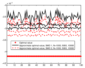
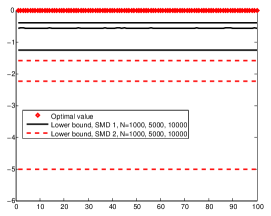
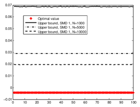
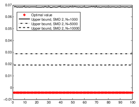
Figure 1: Approximate optimal value, upper and lower bounds for ${\mathcal{C}}_{\tt{SMD\,1}}$ and ${\mathcal{C}}_{\tt{SMD\,2}}$, on 100 instances of problem (2.16) of size $n=100$.

Finally, we consider for parameter $\theta$ involved in the computation of ${\mathcal{C}}_{\tt SMD\,2}$ the range of values $0.005$, $0.01$, $0.05$, $0.1$, $0.5$, $1$, $5$, $10$ considered in [18]. For these values of $\theta$, the average ratios of ${\mathcal{C}}_{\tt SMD\,2}$ and ${\mathcal{C}}_{\tt SMD\,1}$ widths are given in Table 4. These average ratios are all above $3.79$ and as high as $11.04$ for $(\theta,N,n)=(0.005,1000,100)$, which shows again that ${\mathcal{C}}_{{\tt{SMD\,2}}}$ is much more conservative than the interval ${\mathcal{C}}_{{\tt{SMD\,1}}}$ proposed in Section 3.2 for this range of values of $\theta$.

	Problem size $n$
(Ratio, $\theta$, $N$)	40	60	80	100
${|{\mathcal{C}}_{{\tt{SMD\,2}}}|/|{\mathcal{C}}_{{\tt{SMD\,1}}}|}$, $\theta=0.005$, $N=1\,000$	10.99	11.01	11.03	11.04
${|{\mathcal{C}}_{{\tt{SMD\,2}}}|/|{\mathcal{C}}_{{\tt{SMD\,1}}}|}$, $\theta=0.01$, $N=1\,000$	7.39	7.39	7.40	7.40
${|{\mathcal{C}}_{{\tt{SMD\,2}}}|/|{\mathcal{C}}_{{\tt{SMD\,1}}}|}$, $\theta=0.05$, $N=1\,000$	4.45	4.45	4.45	4.46
${|{\mathcal{C}}_{{\tt{SMD\,2}}}|/|{\mathcal{C}}_{{\tt{SMD\,1}}}|}$, $\theta=0.1$, $N=1\,000$	4.06	4.07	4.07	4.08
${|{\mathcal{C}}_{{\tt{SMD\,2}}}|/|{\mathcal{C}}_{{\tt{SMD\,1}}}|}$, $\theta=0.5$, $N=1\,000$	3.79	3.81	3.81	3.82
${|{\mathcal{C}}_{{\tt{SMD\,2}}}|/|{\mathcal{C}}_{{\tt{SMD\,1}}}|}$, $\theta=1$, $N=1\,000$	3.82	3.84	3.85	3.85
${|{\mathcal{C}}_{{\tt{SMD\,2}}}|/|{\mathcal{C}}_{{\tt{SMD\,1}}}|}$, $\theta=5$, $N=1\,000$	4.36	4.38	4.39	4.40
${|{\mathcal{C}}_{{\tt{SMD\,2}}}|/|{\mathcal{C}}_{{\tt{SMD\,1}}}|}$, $\theta=10$, $N=1\,000$	5.07	5.10	5.11	5.12

Table 4: Average ratio of the widths of confidence intervals ${\mathcal{C}}_{{\tt{SMD\,1}}}$ and ${\mathcal{C}}_{{\tt{SMD\,2}}}$, problem (2.16).

5.1.2 Comparison of the confidence intervals on a risk-averse problem

We reproduce the experiments of the previous section for problem (2.17) with $\|\cdot\|=\|\cdot\|_{*}=\|\cdot\|_{2}$ and the distance-generating function $\omega(x)=\omega_{1}(x)=\frac{1}{2}\|x\|_{2}^{2}$. We take $M_{*}=\sqrt{\alpha_{1}^{2}(1-\frac{1}{\varepsilon})^{2}+n(\alpha_{0}+\frac{\alpha_{1}}{\varepsilon})^{2}}$, and two sets of values for $(\alpha_{0},\alpha_{1},\varepsilon)$: $(\alpha_{0},\alpha_{1},\varepsilon)=(0.9,0.1,0.9)$ and the more risk-averse variant $(\alpha_{0},\alpha_{1},\varepsilon)=(0.1,0.9,0.1)$.

For these problems, we first discretize $\xi$, generating a sample of size $10^{5}$ which becomes the sample space. We compute the optimal value of (2.17) using this sample and sample from this set of scenarios to generate the problem instances.

For different problem and sample sizes, we generate again 500 instances. Coverage probabilities of the non-asymptotic confidence intervals are equal to one for all parameter combinations. The time required to compute these confidence intervals is given in Table 5 while the the average ratios of the widths of $\mathcal{C}_{\tt{SMD\,2}}$ and $\mathcal{C}_{\tt{SMD\,1}}$ are reported in Table 6.

Confidence interval and	$\varepsilon=0.1$, problem size				$\varepsilon=0.9$, problem size
sample size $N$	41	61	81	101	41	61	81	101
${\mathcal{C}}_{{\tt{SMD\,1}}}$, $N=100$	0.057	0.069	0.073	0.094	0.058	0.065	0.071	0.082
${\mathcal{C}}_{{\tt{SMD\,2}}}$, $N=100$	0.057	0.064	0.069	0.094	0.055	0.062	0.066	0.074
${\mathcal{C}}_{{\tt{SMD\,1}}}$, $N=10\,000$	5.74	6.13	6.92	7.47	5.79	6.59	7.22	7.97
${\mathcal{C}}_{{\tt{SMD\,2}}}$, $N=10\,000$	5.97	6.41	7.22	7.81	5.85	6.63	7.28	8.00

Table 5: CVaR optimization (problem (2.17)). Average computational time (in seconds) of a confidence interval estimated computing 500 confidence intervals.

Ratio and	$\varepsilon=0.1$, problem size				$\varepsilon=0.9$, problem size
sample size $N$	41	61	81	101	41	61	81	101
${|{\mathcal{C}}_{{\tt{SMD\,2}}}|/|{\mathcal{C}}_{{\tt{SMD\,1}}}|},N=100$	2.29	2.30	2.31	2.31	2.29	2.30	2.31	2.32
${|{\mathcal{C}}_{{\tt{SMD\,2}}}|/|{\mathcal{C}}_{{\tt{SMD\,1}}}|},N=10\,000$	2.30	2.30	2.30	2.31	2.31	2.31	2.32	2.31

Table 6: CVaR optimization (problem (2.17)). Average ratio of the widths of the confidence intervals ${\mathcal{C}}_{{\tt{SMD\,2}}}$ and ${\mathcal{C}}_{{\tt{SMD\,1}}}$.

We observe again on this problem that $\mathcal{C}_{\tt{SMD\,2}}$ is much more conservative than $\mathcal{C}_{\tt{SMD\,1}}$ and for $N=10\,000$ that $\mathcal{C}_{\tt{SMD\,1}}$ is computed quicker than $\mathcal{C}_{\tt{SMD\,1}}$ for all problem sizes. When $\epsilon$ is small and more weight is given to the CVaR, the optimization problem becomes more difficult, i.e., we need a large sample size to obtain a solution of good quality. This can be seen in Figures 2 and 3.

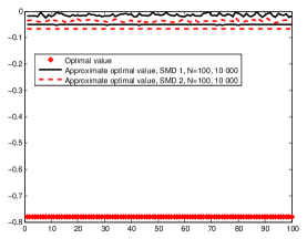
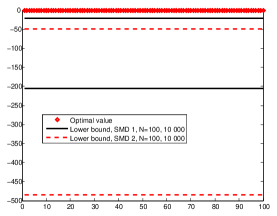
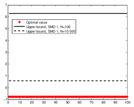
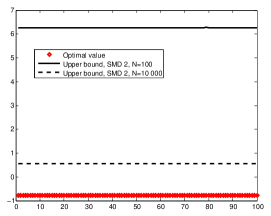
Figure 2: CVaR optimization (problem (2.17)). Approximate optimal value $g^{N}$, upper and lower bounds of $\mathcal{C}_{\tt{SMD\,2}}$ and $\mathcal{C}_{\tt{SMD\,1}}$ on 100 instances, problem size $n=100$ and $\varepsilon=0.1$.

On the top left plots of Figures 2 and 3, for a problem of size $n=100$, we plot 100 realizations of the approximate optimal values $g^{N}$ using variants SMD 1 and SMD 2 of SMD for two sample sizes: $N=100$ and $N=10\,000$ ($\varepsilon=0.1$ for Figure 2 and $\varepsilon=0.9$ for Figure 2). For fixed sample size $N$, for $\varepsilon=0.9$ these realizations are much closer to the optimal value than for $\varepsilon=0.1$. On the remaining plots of Figure 2 and 3, we report the upper and lower bounds of confidence intervals $\mathcal{C}_{\tt{SMD\,1}}$ and $\mathcal{C}_{\tt{SMD\,2}}$. We observe again that (i) upper (resp. lower) bounds decrease (resp. increase) when the sample size increases, (ii) $\mathcal{C}_{\tt{SMD\,2}}$ and $\mathcal{C}_{\tt{SMD\,1}}$ upper bounds are very close, and (iii) $\mathcal{C}_{\tt{SMD\,1}}$ lower bound is much larger than $\mathcal{C}_{\tt{SMD\,2}}$ lower bound (reflecting the fact that $\mathcal{C}_{\tt{SMD\,2}}$ is much more conservative than $\mathcal{C}_{\tt{SMD\,1}}$). Additionally, we observe that when $\epsilon$ is small ($\varepsilon=0.1$) and more weight is given to the CVaR ($\alpha_{1}=0.9$) the upper and lower bounds become more distant to the optimal value, i.e., the width of the confidence intervals increases.

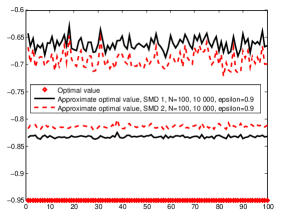
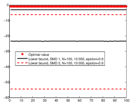
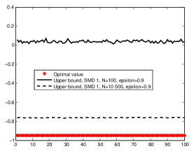
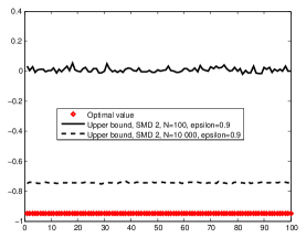
Figure 3: CVaR optimization (problem (2.17)). Approximate optimal value $g^{N}$, upper and lower bounds of $\mathcal{C}_{\tt{SMD\,2}}$ and $\mathcal{C}_{\tt{SMD\,1}}$ on 100 instances, problem size $n=100$ and $\varepsilon=0.9$.

To conclude, confidence intervals ${\mathcal{C}}_{\tt SMD\,1}$ and ${\mathcal{C}}_{\tt SMD\,2}$ cannot be compared directly because both the constants involved and the steps used to generate the points $x_{1},\ldots,x_{N}$, are different. However, we hypothesize that the optimization in ${\tt SMD\,2}$ results in both the conservativeness and the computation time difference.

5.2 Comparing the multistep and nonmultistep variants of SMD to solve problem (2.16)

We solve various instances of problem (2.16) (with $a=1,b=0$) using SMD and its multistep version defined in Section 4 taking $\omega(x)=\omega_{2}(x)=\frac{1}{2}\|x\|_{2}^{2}$. These algorithms in this case are the RSA and multistep RSA. We fix the parameters $\alpha_{1}=0.9,\alpha_{0}=0.1,\lambda_{0}=4,x_{1}=[1;0;\ldots;0]],D_{X}=\sqrt{2}$, and recall that $\mu(\omega)=\mu(\omega_{2})=M(\omega_{2})=\mu(f)=1,\rho=2$, $L=|\alpha_{0}|\sqrt{n}+\alpha_{1}(\sqrt{n}+\lambda_{0})$, $M_{1}=2|\alpha_{0}|+0.5\alpha_{1}$, and $M_{2}=2\sqrt{n}(|\alpha_{0}|+\alpha_{1})$. In this and the next section, $\xi$ is again a random vector with i.i.d. Bernoulli entries: ${\hbox{\rm Prob}}(\xi_{i}=1)=\Psi_{i},\;{\hbox{\rm Prob}}(\xi_{i}=-1)=1-\Psi_{i}$, with $\Psi_{i}$ randomly drawn over $[0,1]$.

We first take $n=100$ and choose the number of iterations using Proposition 4.5, namely we take $N=\lceil 1+78A(f,\omega_{2})\rceil=312\,248$ which ensures that for the MSSMD algorithm $\mathbb{E}\Big{[}\Big{|}f(y_{{\tt{Steps}}+1})-f(x_{*})\Big{|}\leq 0.1$. (we also check that for this value of $N$, relation (4.76) (an assumption of Proposition 4.5) holds). For this value of $N$, the values of $\gamma^{t}$ for each iteration of the MSSMD algorithm as well as the constant value of $\gamma$ for the SMD algorithm are represented in the left plot of Figure 4. We observe that the MSRSA algorithm starts with larger steps (when we are still far from the optimal solution) and ends with smaller steps (when we get closer to the optimal solution) than the RSA algorithm. We run each algorithm 50 times and report in the middle plot of Figure 4 the average (over the 50 runs) of the approximate optimal values computed along the iterations with both algorithms. We also report in the right plot of Figure 4 the average (over these 50 runs) of the value of the objective function at the SMD and MSSMD solutions.

More precisely, for each run of the SMD algorithm, for iteration $i$ the approximate optimal value is $g^{i}=\frac{1}{i}\sum_{k=1}^{i}g(x_{k},\xi_{k})$ (defined in Algorithm 1) while for iteration $j$ of the $i$-th step of the MSSMD algorithm, the approximate optimal value is $g^{i,j}=\frac{1}{j}\sum_{k=1}^{j}g(x_{i,k},\xi_{i,k})$ (defined in Algorithm 3) where $\xi_{i,k}$ and $x_{i,k}$ are respectively the $k$-th realization of $\xi$ and the $k$-th point generated for that step $i$ (of course, for a given run, the same samples are used for SMD and MSSMD).

We observe that we get better (lower) approximations of the optimal value using the MSRSA algorithm. After a large number of iterations, the algorithms provide very close approximations of the optimal value (themselves close to the optimal value of the problem), which is in agreement with the results of Sections 3 and 4 which state that for both algorithms the approximate optimal values converge in probability to the optimal value of the problem. However, it is observed that the MSRSA algorithm provides an approximate solution of good quality much quicker than the RSA algorithm.

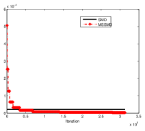
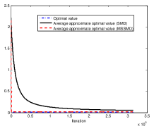
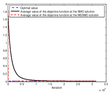
Figure 4: Steps (left plot), average (computed over 50 runs) approximate optimal values (middle plot), and average (computed over 50 runs) value of the objective function at the solution (right plot) along the iterations of the SMD and MSSMD algorithms run on problem (2.16) with $n=100$, $N=312\,248$.

We also observe that if the value of the sample size $N=312\,248$ chosen based on Proposition 4.5 indeed allows us to solve the problem with a good accuracy, it is very conservative. In a second series of experiments, we choose various problem sizes $n$ and smaller sample sizes $N$, namely $(n,N)=(50,1000),(n,N)=(100,1000),(n,N)=(500,10\,000)$, and $(n,N)=(1000,10\,000)$, still observing solutions of good quality. For these values of the pair $(n,N)$, the values of the steps used for the SMD and MSSMD algorithms are reported in Figure 5. Here again the MSRSA algorithm starts with larger steps and ends with smaller steps.

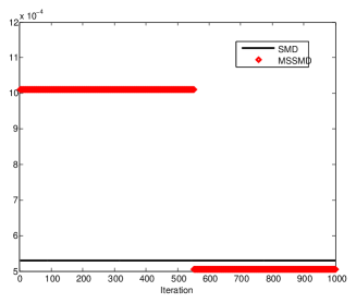
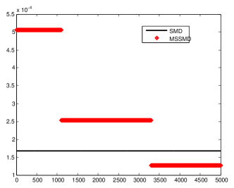
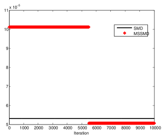
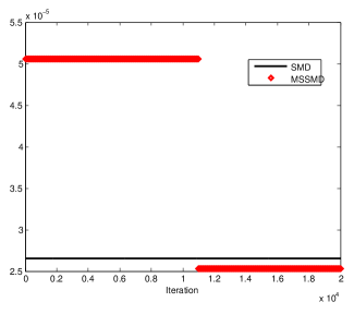
Figure 5: Steps used for the SMD and MSSMD algorithms to solve problem (2.16) with $(n,N)=(50,1000)$ (top left plot), $(n,N)=(100,5000)$ (top right plot), $(n,N)=(500,10\,000)$ (bottom left), $(n,N)=(1000,10\,000)$ (bottom right).

The average (over 50 runs) of the approximate optimal value and of the value of the objective function at the SMD and MSSMD solutions are reported in Figures 6 and 7. We still observe on these simulations that MSSMD allows us to obtain a solution of good quality much quicker than SMD and ends up with a better solution, even when only two different step sizes are used for MSSMD.

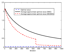
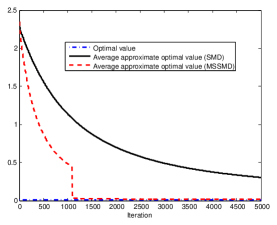
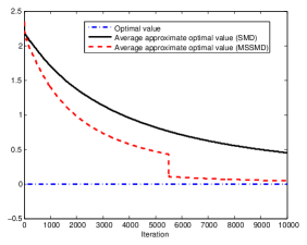
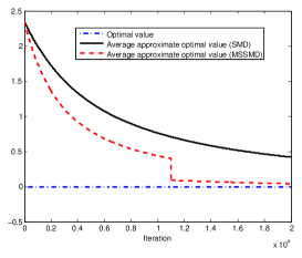
Figure 6: Average over 50 realizations of the approximate optimal values computed by the SMD and MSSMD algorithms to solve (2.16). Top left: $(n,N)=(50,1000)$, top right: $(n,N)=(100,5000)$, bottom left: $(n,N)=(500,10\,000)$, bottom right: $(n,N)=(1000,10\,000)$.

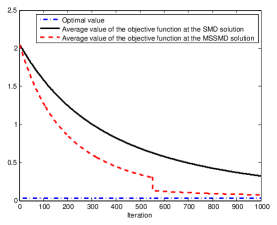
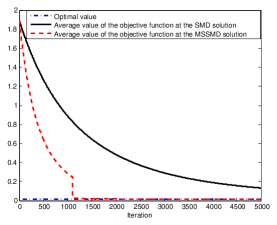
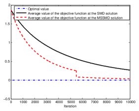
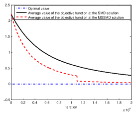
Figure 7: Average over 50 realizations of the values of the objective function at the approximate solutions computed by the SMD and MSSMD algorithms to solve (2.16). Top left: $(n,N)=(50,1000)$, top right: $(n,N)=(100,5000)$, bottom left: $(n,N)=(500,10\,000)$, bottom right: $(n,N)=(1000,10\,000)$.

5.3 Comparing the multistep and nonmultistep variants of SMD to solve problem (2.18)

We reproduce the experiment of the previous section running 50 times SMD and MSSMD on problem (2.18) taking $\omega(x)=\omega_{2}(x)=\frac{1}{2}\|x\|_{2}^{2}$, $\varepsilon=0.9$, $\alpha_{1}=0.1,\alpha_{0}=0.9,\lambda_{0}=1,x_{1}=[0;1;0;\ldots;0]],D_{X}=\sqrt{3}$, and recall that $\mu(\omega)=\mu(\omega_{2})=M(\omega_{2})=\mu(f)=1,\rho=2$, $L=\sqrt{\alpha_{1}^{2}(1-\frac{1}{\varepsilon})^{2}+n(\alpha_{0}+\frac{\alpha_{1}}{\varepsilon})^{2}}+2\lambda_{0}$, $M_{1}=2(\alpha_{0}+\frac{\alpha_{1}}{\varepsilon})$, and $M_{2}=\sqrt{\left(\frac{\alpha_{1}}{\varepsilon}\right)^{2}+4n\left(\alpha_{0}+\frac{\alpha_{1}}{\varepsilon}\right)^{2}}$. We consider again four combinations for the pair $(n,N)$: $(n,N)=(50,1000),(100,1000),(500,10\,000)$, and $(1000,10\,000)$.

The steps used along the iterations of the SMD and MSSMD algorithms are reported in Figure 8.

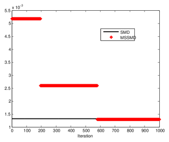
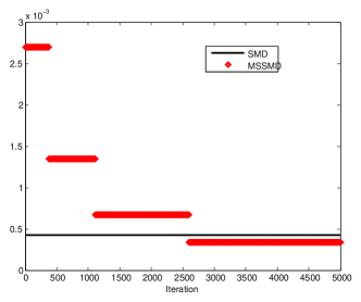
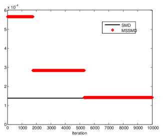
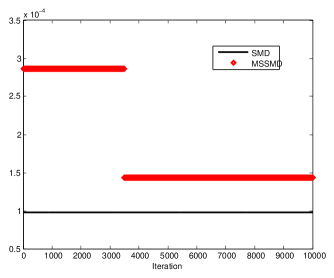
Figure 8: Steps used for the SMD and MSSMD algorithms to solve problem (2.18) with $(n,N)=(50,1000)$ (top left plot), $(n,N)=(100,5000)$ (top right plot), $(n,N)=(500,10\,000)$ (bottom left), $(n,N)=(1000,10\,000)$ (bottom right).

The average (computed running the algorithms 50 times) of the approximate optimal values and of the value of the objective function at the approximate solutions are reported in Figures 9 and 10. In these experiments we observe again that MSSMD approximate solutions are better along the iterations and at the end of the optimization process.

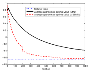
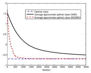
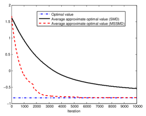
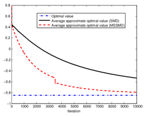
Figure 9: Average over 50 realizations of the approximate optimal values computed by the SMD and MSSMD algorithms to solve (2.18). Top left: $(n,N)=(50,1000)$, top right: $(n,N)=(100,5000)$, bottom left: $(n,N)=(500,10\,000)$, bottom right: $(n,N)=(1000,10\,000)$.

6 Conclusion and future work

We derived a new confidence interval on the optimal value of a convex stochastic program using the SMD algorithm that has the advantage of being quicker to compute and much less conservative than previous confidence intervals.

We introduced a multistep extension of the SMD algorithm and derived a computable nonasymptotic confidence interval on the optimal value of a risk-averse stochastic program, expressed in terms of EPRM, using this algorithm. We have shown (using two stochastic optimization problems) that the multistep SMD algorithm can obtain “good” solutions much quicker that the SMD algorithm.

Our work is applicable to obtain confidence intervals on the risk measure value of a distribution on the basis of a sample from this distribution, if this risk measure is an EPRM.

The analysis presented in this paper can be extended in several ways.

First, numerical tests could be performed to analyze the quality of the confidence intervals given by Corollary 4.7 for multistep SMD. Other algorithms could be considered to solve (1.1) and the corresponding confidence intervals derived. More general classes of problems, for instance involving integer variables, could also be analyzed.

Next, we could take a law invariant coherent risk measure for $\mathcal{R}$ in (1.1). In this situation, asymptotic confidence intervals on the optimal value of (1.1) could be obtained combining the Central Limit Theorem for risk measures given in [25], the Delta theorem, and the Functional Central Limit Theorem.

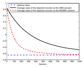
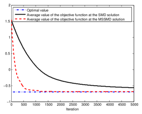
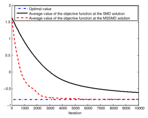
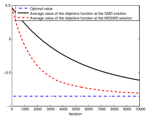
Figure 10: Average over 50 realizations of the values of the objective function at the approximate solutions (right plots) computed by the SMD and MSSMD algorithms to solve (2.18). Top left: $(n,N)=(50,1000)$, top right: $(n,N)=(100,5000)$, bottom left: $(n,N)=(500,10\,000)$, bottom right: $(n,N)=(1000,10\,000)$.

Finally, our analysis can be used to study the following problem: defining

$$\rho_{i}(\xi)=\left\{\begin{array}[]{l}\min\;f(x):=\mathcal{R}_{i}\left[g(x,\xi)\right],\\ x\in X\end{array}\right.$$ (6.88)

for an EPRM $\mathcal{R}_{i}$ and given samples from the distributions of random vectors $\xi_{1},\ldots,\xi_{m}$, our developments can be used to compare the optimal values $\rho_{i}(\xi_{i}),\,i=1,\ldots,m$, studying the following statistical tests:

$$\begin{array}[]{ll}(a)\;H_{0}:\;\rho_{1}(\xi_{1})=\rho_{2}(\xi_{2})=\ldots=\rho_{m}(\xi_{m})&\mbox{against }{\overline{H_{0}}},\\ (b)\;H_{0}^{i}:\;\rho_{i}(\xi_{i})\leq\rho_{j}(\xi_{j}),\;\;1\leq j\neq i\leq m&\mbox{against }{\overline{H_{0}^{i}}},\\ (c)\;H_{0}:\;\rho_{1}(\xi_{1})\leq\rho_{2}(\xi_{2})\leq\ldots\leq\rho_{m}(\xi_{m})&\mbox{against }{\overline{H_{0}}},\end{array}$$ (6.89)

where ${\overline{H_{0}}}$ is the complement of $H_{0}$. Without assuming the independence of $\xi_{1},\ldots,\xi_{m}$, a special case of (6.89) is obtained taking a singleton $X=\{x^{*}_{i}\}$ for the set $X$ defining $\rho_{i}$, fixing the risk measure $\mathcal{R}_{i}=\mathcal{R}$ and the distribution $\xi_{i}=\xi$. Setting $\eta_{i}=g(x^{*}_{i},\xi)$, test (6.89) boils down in this case to

$$\begin{array}[]{ll}\begin{array}[]{ll}(a)\;H_{0}:\;\mathcal{R}(\eta_{1})=\mathcal{R}(\eta_{2})=\ldots=\mathcal{R}(\eta_{m})&\mbox{against }{\overline{H_{0}}},\\ (b)\;H_{0}^{i}:\;\mathcal{R}(\eta_{i})\leq\mathcal{R}(\eta_{j}),\;\;1\leq j\neq i\leq m&\mbox{against }{\overline{H_{0}^{i}}},\\ (c)\;H_{0}:\;\mathcal{R}(\eta_{1})\leq\mathcal{R}(\eta_{2})\leq\ldots\leq\mathcal{R}(\eta_{m})&\mbox{against }{\overline{H_{0}}}.\end{array}\end{array}$$ (6.90)

These tests are useful when we want to choose among $m$ candidate solutions $x^{*}_{1},\ldots,x^{*}_{m}$ for the problem

$$\left\{\begin{array}[]{l}\min\;f(x):=\mathcal{R}\left[g(x,\xi)\right],\\ x\in X,\end{array}\right.$$

the best one (the one with the smallest risk measure value), using risk measure $\mathcal{R}$ to rank the distributions $\eta_{i}$.

Acknowledgments. The author would like to thank Arkadi Nemirovski, Anatoli Juditsky, and Alexander Shapiro for helpful discussions. The author’s research was partially supported by an FGV grant, CNPq grant 307287/2013-0, FAPERJ grants E-26/110.313/2014 and E-26/201.599/2014.

Appendix

We have collected in the Appendix two proofs, essentially known, see [21].

Proof of Lemma 3.2..

We first show that for any $\gamma>0$ and $\tau=1,\ldots,N$, we have

$${\mathbb{E}}_{|\tau-1}\Big{[}\exp\{\gamma\eta_{\tau}\}\Big{]}\leq\exp\{\gamma^{2}\}.$$ (6.91)

Let us fix $0<\gamma\leq 1$. Observing that

$$e^{x}\leq x+e^{x^{2}}\mbox{ for every }x\in\mathbb{R},$$ (6.92)

we obtain

$$\begin{array}[]{lll}{\mathbb{E}}_{|\tau-1}\Big{[}\exp\{\gamma\eta_{\tau}\}\Big{]}&\leq&{\mathbb{E}}_{|\tau-1}\Big{[}\gamma\eta_{\tau}\Big{]}+{\mathbb{E}}_{|\tau-1}\Big{[}\exp\{\gamma^{2}\eta_{\tau}^{2}\}\Big{]}\vspace*{0.1cm}\\ &\leq&{\mathbb{E}}_{|\tau-1}\Big{[}\exp\{\gamma^{2}\eta_{\tau}^{2}\}\Big{]}\mbox{ using }\eqref{martin}\\ &\leq&{\mathbb{E}}_{|\tau-1}\Big{[}(\exp\{\eta_{\tau}^{2}\})^{\gamma^{2}}\Big{]}\leq\left({\mathbb{E}}_{|\tau-1}\Big{[}\exp\{\eta_{\tau}^{2}\}\Big{]}\right)^{\gamma^{2}},\end{array}$$

where the last inequality is Jensen inequality applied to the concave function $x^{\gamma^{2}}$. Plugging (3.35) into the above inequality shows that (6.91) holds for $0<\gamma\leq 1$.

For $\gamma>1$,

$$\begin{array}[]{lll}{\mathbb{E}}_{|\tau-1}\Big{[}\exp\{\gamma\eta_{\tau}\}\Big{]}&\leq&{\mathbb{E}}_{|\tau-1}\Big{[}\exp\{{1\over 2}\gamma^{2}+{1\over 2}\eta_{\tau}^{2}\}\Big{]}\vspace*{0.1cm}\\ &\leq&\exp\{\frac{\gamma^{2}}{2}\}\sqrt{{\mathbb{E}}_{|\tau-1}\Big{[}\exp\{\eta_{\tau}^{2}\}\Big{]}}\leq\exp\{\frac{\gamma^{2}+1}{2}\}\leq\exp\{\gamma^{2}\},\end{array}$$

where we have used (3.35) for the third inequality and the fact that $\gamma>1$ for the last one. We have thus shown that (6.91) holds for every $\gamma>0$. As a result, for $\gamma>0$, setting $S_{\tau}=\sum_{s=1}^{\tau}\eta_{s}$, we have

$$\begin{array}[]{lll}{\mathbb{E}}\Big{[}\exp\{\gamma S_{\tau}\}\Big{]}&=&{\mathbb{E}}\Big{[}\exp\{\gamma S_{\tau-1}\}{\mathbb{E}}_{|\tau-1}\Big{[}\exp\{\gamma\eta_{\tau}\}\Big{]}\Big{]}\\ &\leq&\exp\{\gamma^{2}\}{\mathbb{E}}\Big{[}\exp\{\gamma S_{\tau-1}\}\Big{]}\mbox{ using }\eqref{expineq0}.\end{array}$$

It follows that for $\gamma>0$

$$\begin{array}[]{lll}{\mathbb{E}}\Big{[}\exp\{\gamma S_{\tau}\}\Big{]}&\leq&\exp\{\gamma^{2}(\tau-1)\}{\mathbb{E}}\Big{[}\exp\{\gamma\eta_{1}\}\Big{]}\leq\exp\{\gamma^{2}\tau\}\mbox{ using }\eqref{expineq0}.\end{array}$$ (6.93)

Next, for $\gamma>0$,

$$\begin{array}[]{lll}\mathbb{P}\Big{(}S_{N}>\Theta\,\sqrt{N}\Big{)}&=&\mathbb{P}\Big{(}\exp\{\gamma S_{N}\}>\exp\{\Theta\,\sqrt{N}\gamma\}\Big{)}\\ &\leq&\displaystyle\min_{\gamma>0}\;\exp\{-\Theta\sqrt{N}\gamma\}{\mathbb{E}}\Big{[}\exp\{\gamma S_{N}\}\Big{]}\mbox{ using Chernoff bound,}\\ &\leq&\exp\{\displaystyle\min_{\gamma>0}\Big{[}\gamma^{2}N-\Theta\sqrt{N}\gamma\Big{]}\}=\exp\{-\Theta^{2}/4\}\mbox{ using }\eqref{bornesupstau}.\end{array}$$

This achieves the proof of inequality (3.36). $\Box$

Proof of Lemma 3.10..

Invoking (3.53), we get

$$\forall y\in X:\gamma_{\tau}e_{\tau}^{\scriptscriptstyle\top}(u_{\tau+1}-y)\leq V_{u_{\tau}}(y)-V_{u_{\tau+1}}(y)-V_{u_{\tau}}(u_{\tau+1}),$$

whence for all $x\in X$, we have

$$\begin{array}[]{rcl}\gamma_{\tau}e_{\tau}^{\scriptscriptstyle\top}(u_{\tau}-y)&\leq&V_{u_{\tau}}(y)-V_{u_{\tau+1}}(y)+\Big{[}\gamma_{\tau}e_{\tau}^{\scriptscriptstyle\top}(u_{\tau}-u_{\tau+1})-V_{u_{\tau}}(u_{\tau+1})\Big{]}\vspace*{0.1cm}\\ &\leq&V_{u_{\tau}}(y)-V_{u_{\tau+1}}(y)+\Big{[}\gamma_{\tau}\|e_{\tau}\|_{*}\|u_{\tau}-u_{\tau+1}\|-{\mu(\omega)\over 2}\|u_{\tau}-u_{\tau+1}\|^{2}\Big{]}\\ &\leq&V_{u_{\tau}}(y)-V_{u_{\tau+1}}(y)+\displaystyle\frac{\gamma_{\tau}^{2}\|e_{\tau}\|_{*}^{2}}{2\mu(\omega)},\\ \end{array}$$

where we have used (3.48) for the second inequality. Summing up the resulting inequalities over $\tau=1,...,N$, and taking into account that $V_{u_{N+1}}(y)\geq 0$ by (3.48) and $V_{u_{1}}(y)\leq{1\over 2}D_{\omega,X}^{2}$ by (3.50) (recall that $u_{1}=x_{\omega}$), we arrive at (3.58). $\Box$

References

- [1] E. D. Andersen and K. D. Andersen. The MOSEK optimization toolbox for MATLAB, manual. Version 7.0, 2013. http://docs.mosek.com/7.0/toolbox/.
- [2] G. Bayraksan and D.P. Morton. Assessing solution quality in stochastic programs. Math. Program., 108:495–514, 2006.
- [3] G. Bayraksan and D.P. Morton. A sequential sampling procedure for stochastic programming. Oper. Res., 59:898–913, 2011.
- [4] G. Bayraksan and P. Pierre-Louis. Fixed-width sequential stopping rules for a class of stochastic programs. SIAM J. Optim., 22:1518–1548, 2012.
- [5] A. Chiralaksanakul and D.P. Morton. Assessing policy quality in multi-stage stochastic programming. Stochastic Programming E-Print Series, 12, 2004.
- [6] J. Dupačova and R.J.-B Wets. Asymptotic behavior of statistical estimators and of optimal solutions of stochastic optimization problems. Ann. Stat., 16:1517–1549, 1988.
- [7] A. Eichhorn and W. Römisch. Polyhedral risk measures in stochastic programming. SIAM J. Optim., 16:69–95, 2005.
- [8] A. Eichorn and W. Römisch. Stochastic integer programming: Limit theorems and confidence intervals. Math. Oper. Res., 32:118–135, 2007.
- [9] S. Ghadimi and G. Lan. Optimal stochastic approximation algorithms for strongly convex stochastic composite optimization i: A generic algorithmic framework. SIAM Journal on Optimization, 22:1469–1492, 2012.
- [10] V. Guigues. Convergence analysis of sampling-based decomposition methods for risk-averse multistage stochastic convex programs. Available on arXiv at http://arxiv.org/abs/1408.4439, 2014.
- [11] V. Guigues, A. Juditsky, and A. Nemirovski. Non-asymptotic confidence bounds for the optimal value of a stochastic program. Available on arXiv at http://arxiv.org/abs/1601.07592, 2016.
- [12] V. Guigues and W. Römisch. Sampling-based decomposition methods for multistage stochastic programs based on extended polyhedral risk measures. SIAM J. Optim., 22:286–312, 2012.
- [13] A. Juditsky and Y. Nesterov. Primal-dual subgradient methods for minimizing uniformly convex functions. Available on arXiv at http://arxiv.org/abs/1401.1792, 2010.
- [14] Anatoli Juditsky and Arkadi Nemirovski. First order methods for nonsmooth convex large-scale optimization, I: general purpose methods. In S. Sra, S. Nowozin, and S.J. Wright, editors, Optimization for Machine Learning, pages 121–148. MIT Press, 2011.
- [15] A.J. King and R.T. Rockafellar. Asymptotic theory for solutions in statistical estimation and stochastic programming. Math. Oper. Res., 18:148–162, 1993.
- [16] A.J. Kleywegt, A. Shapiro, and T. Homem de Mello. The sample average approximation method for stochastic discrete optimization. SIAM J. Optim., 12:479–502, 2001.
- [17] A.J. Kleywegt, A. Shapiro, and T. Homem de Mello. The sample average approximation method for stochastic programs with integer recourse. Optimization OnLine, 2002.
- [18] G. Lan, A. Nemirovski, and A. Shapiro. Validation analysis of mirror descent stochastic approximation method. Math. Program., 134:425–458, 2012.
- [19] W.K. Mak, D.P. Morton, and R.K. Wood. Monte Carlo bounding techniques for determining solution quality in stochastic programs. Oper. Res. Lett., 24:47–56, 1999.
- [20] A. Nedich and S. Lee. On stochastic subgradient mirror-descent algorithm with weighted averaging. SIAM Journal on Optimization, 24:84–107, 2014.
- [21] A. Nemirovski, A. Juditsky, G. Lan, and A. Shapiro. Robust stochastic approximation approach to stochastic programming. SIAM J. Optim., 19:1574–1609, 2009.
- [22] M.V.F. Pereira and L.M.V.G Pinto. Multi-stage stochastic optimization applied to energy planning. Math. Program., 52:359–375, 1991.
- [23] G. Pflug. Asymptotic stochastic programs. Math. Oper. Res., 20:769–789, 1995.
- [24] G. Pflug. Stochastic programs and statistical data. Ann. Oper. Res., 85:59–78, 1999.
- [25] G. Pflug and N. Wozabal. Asymptotic distribution of law-invariant risk functionals. Finance Stoch, 14:397–418, 2010.
- [26] B.T. Polyak. New stochastic approximation type procedures. Automat. i Telemekh (English translation: Automation and Remote Control), 7:98–107, 1990.
- [27] B.T. Polyak and A. Juditsky. Acceleration of stochastic approximation by averaging. SIAM J. Contr. and Optim., 30:838–855, 1992.
- [28] A. Rakhlin, O. Shamir, and K. Sridharan. Making gradient descent optimal for strongly convex stochastic optimization. 29th International Conference on Machine Learning (ICML), 2012.
- [29] H. Robbins and S. Monroe. A stochastic approximation method. Annals of Math. Stat., 22:400–407, 1951.
- [30] R.T. Rockafellar and S. Uryasev. Conditional Value-at-Risk for general loss distributions. J. Bank. Financ., 26(7):1443–1471, 2002.
- [31] W. Römisch. Delta method, infinite dimensional. In S. Kotz, C. B. Read, N. Balakrishnan, B. Vidakovic, eds. Extended entry, Encyclopedia of Statistical Sciences, 2nd ed., Wiley, New York., 2005.
- [32] W. Römisch and R. Schultz. Stability of solutions for stochastic programs with complete recourse. Math. Oper. Res., 18:590–609, 1993.
- [33] R. Schultz. Strong convexity in stochastic programs with complete recourse. Journal of Computational and Applied Mathematics, 56:3–22, 1994.
- [34] A. Shapiro. Asymptotic properties of statistical estimators in stochastic programming. Ann. Statist., 17:841–858, 1989.
- [35] A. Shapiro. Asymptotic analysis of stochastic programs. Ann. Oper. Res., 30:169–186, 1991.
- [36] A. Shapiro and T. Homem de Mello. On rate of convergence of optimal solutions of Monte Carlo approximations of stochastic programs. SIAM J. Optim., 11:70–86, 2000.
- [37] A. Shapiro, D. Dentcheva, and A. Ruszczyński. Lectures on Stochastic Programming: Modeling and Theory. SIAM, Philadelphia, 2009.
- [38] M. Talagrand. Sharper bounds for Gaussian and empirical processes. Ann. Probab., 22:28–76, 1994.
- [39] M. Talagrand. The Glivenko-Cantelli problem, ten years later. J. Theoret. Probab., 9:371–384, 1996.