Optimization of starshades: focal plane versus pupil plane

Abstract

Aims. We search for the best possible transmission for an external occulter coronagraph that is dedicated to the direct observation of terrestrial exoplanets. We show that better observation conditions are obtained when the flux in the focal plane is minimized in the zone in which the exoplanet is observed, instead of the total flux received by the telescope.

Methods. We describe the transmission of the occulter as a sum of basis functions. For each element of the basis, we numerically computed the Fresnel diffraction at the aperture of the telescope and the complex amplitude at its focus. The basis functions are circular disks that are linearly apodized over a few centimeters (truncated cones). We complemented the numerical calculation of the Fresnel diffraction for these functions by a comparison with pure circular discs (cylinder) for which an analytical expression, based on a decomposition in Lommel series, is available. The technique of deriving the optimal transmission for a given spectral bandwidth is a classical regularized quadratic minimization of intensities, but linear optimizations can be used as well.

Results. Minimizing the integrated intensity on the aperture of the telescope or for selected regions of the focal plane leads to slightly different transmissions for the occulter. For the focal plane optimization, the resulting residual intensity is concentrated behind the geometrical image of the occulter, in a blind region for the observation of an exoplanet, and the level of background residual starlight becomes very low outside this image. Finally, we provide a tolerance analysis for the alignment of the occulter to the telescope which also favors the focal plane optimization.This means that telescope offsets of a few decimeters do not strongly reduce the efficiency of the occulter.

1 Introduction

Almost twenty years ago Mayor & Queloz (1995) made the first detection of an exoplanet, and more than a thousand are now recognized. External occulters will be formidable instruments for performing detailed spectral analysis of exo-Earths that have previously been detected by other methods.

The first use of an external occulter dates back to Evans (1948), who used an occulting disk set in front of a very small coronagraph of Lyot (1939). Very soon solar astronomers have identified diffraction effects of a circular occulter and considered various kinds of apodized, shaped, or multiple occulters for space missions, as well described in the review paper of Koutchmy (1988). Because of implementation difficulties, toothed or multiple discs are preferred over radially graded ones, which have been described in Purcell & Koomen (1962) and Newkirk Jr & Bohlin (1965). Next to the successful Solar and Heliospheric Observatory mission (Brueckner et al. (1995)), future solar coronagraphy envisages formation-flying spacecrafts with an occulter of diameter 1.5 m at about 150 m in front of a small telescope (Vives et al. (2009)).

The parameters are completely different for exoplanets,. In rounded numbers, the occulting angle is about 0.2 arcsec against 2000 arcsec for the Sun, and a large 4m diameter telescope is needed with an occulter of 50 m diameter at a distance of 80 000 km. The positive aspect of exoplanet experiments is that diffraction phenomena are less difficult to simulate numerically than in the solar case. This is due to two reasons. There are fewer than 20 Fresnel zones compared with 8000 in the solar case, and the main source of diffracted light is a point source instead of a huge $1/2^{\circ}$ extended object. Nevertheless, the problem remains difficult because of the high expected dynamic range.

Progression of ideas for exoplanets first followed developments for the Sun, with little interaction, but now the theoretical calculations and instrumental developments have resulted in much more developments than in the solar case. In his review of space astronomy Spitzer (1962) mentioned the technique of apodization envisaged by solar astronomers. Elaborated petal-shaped occulters can already be found in Marchal (1985), and Copi & Starkman (2000) proposed a circular apodizing transmission on a square mask. Studies of shaped and apodized occulters have been reported in many publications, such as Cash (2006), Arenberg et al. (2007), Vanderbei et al. (2007), Soummer et al. (2010), Cash (2011) and Wasylkiwskyj & Shiri (2011), to cite just a few. Although partially transparent petal shaped occulters are envisaged by Shiri & Wasylkiwskyj (2013), the most advanced technological developments are for petaled star shades. The two-step procedure leading to an optimal shaped occulter is well described in Kasdin et al. (2013). These authors explained that they first seek for the optimal variable transmission of an apodized occulter and then chose a sufficient number of petals for the shaped occulter to best approach the theoretical result given by the variable transmission. We here focus only on the first part of this approach, that is, on the search for an ideal transmission, leaving the final design of a shaped occulter to a future work.

Our purpose is to show that the occulter can be optimized advantageously from the telescope focal plane, which will minimize the level of light that is diffracted by the star in a zone of interest of the focal plane for the exoplanet. The resulting illumination on the telescope aperture appears to be apodized from center to edge. The integrated flux on the telescope pupil is no longer minimized. The observation is nevertheless improved because most of the residual flux is trapped behind the geometrical image of the mask, in a blind area for the observation of the exoplanet. Differences in transmission with an occulter that minimizes the flux over the aperture are small, but the gain in the residual background light at the level of the exoplanet range from 1.9 to 50 depending on the spectral bandwidth, which might correspond to a gain in integration time of a factor 3.6 to 2500 for certain observing conditions, in photon counting mode.

The paper is organized as follows: The fundamental relations that describe the complex amplitudes diffracted by the occulter in the aperture and focal planes are given in Sect. 2. The procedure for optimizing the transmission of a circularly symmetric apodized occulter to minimize the flux on the telescope aperture or for selected regions of the focal plane are described in Sect. 3. Sect. 4 contains results on the optimization problem and a discussion. Additional information is given in two appendices based on an analytic approach of the Fresnel diffraction of a pure circular disc and of a linearly apodized disc.

2 Expressions of complex amplitudes and intensities in the aperture and focal planes

We denote with $2\Omega$ the overall diameter of the occulter. For an occulting mask, it is convenient to write its transmission as $t(r)=1-f(r)$, with the attenuation function $f(r)$ constrained by $0\leq f(r)\leq 1$ for $|r|\leq\Omega$, and $f(r)=0$ for $|r|>\Omega$. For a wave of unit amplitude, the Fresnel diffraction at the telescope aperture at a distance $z$ from the occulter (see Fig. 1) can be written as

$$\psi(r)=1-\frac{\tau_{z}(r)}{i\lambda z}\int_{0}^{\Omega}2\pi\xi f(\xi)\tau_{z}(\xi)J_{0}(2\pi\frac{\xi r}{\lambda z})d\xi,$$ (1)

where $\tau_{z}(r)=\exp(i\pi r^{2}/\lambda z)$ is a quadratic phase-term corresponding to a diverging lens, and $J_{0}(r)$ is the Bessel function of the first kind.

This relation is equivalent to Eq. 4 of Vanderbei et al. (2007), neglecting here the term of propagation of a plane wave. In general, this integral does not admit an analytical solution, except for $f(r)=1$, as shown by Aime (2013) and outlined here in Appendix A. Therefore, Eq.1, which appears as the Hankel transform of $f(r)\tau_{z}(r)$, must be evaluated numerically. Computations of these transforms are delicate, as discussed by Lemoine (1994) for example, who recommended a sampling of the function based on zeroes of the Bessel function $J_{0}$. In practice, after several tests described in Appendix A and B and below, we directly used the function NIntegrate of Mathematica, which performs very well for this kind of calculation, thanks to recent improvements of numerical integration.

This wavefront $\psi(r)$ arrives onto the aperture of the telescope of transmission $P(r)$, and we denote with $\varphi(r)=P(r)\;\psi(r)$ the complex amplitude of the wave going through the telescope aperture. For the sake of simplicity, we assume in the following a perfectly circular telescope of diameter $2R$, centered on the optical axis of the system, so that $P(r)=\Pi(r/R)$, defining here for convenience that the box distribution $\Pi(r)$ equals 1 for $|r|<1$ and 0 elsewhere. Note that a more realistic telescope with a central obscuration can be easily inserted into the calculations. Using the circular symmetry of the problem, the complex amplitude of the wave in the focal plane can be written as a Hankel transform of $\varphi(r)$ of the form:

$$\phi(r)=\frac{\tau_{F}(r)}{i\lambda F}\int_{0}^{R}2\pi\xi\varphi(\xi)J_{0}(2\pi\frac{\xi r}{\lambda F})d\xi=\frac{\tau_{F}(r)}{i\lambda F}\hat{\varphi}(\frac{r}{\lambda F}),$$ (2)

where $F$ is the focal length of the telescope. Note that here the phase term $\tau_{F}(r)$ is compensated for by the lens phase function of the telescope, meaning that a simple 2D Fourier transform or Hankel transform denoted by $\hat{\varphi}$ substitutes the more complex Fresnel propagation of Eq. 1.

It is moreover convenient to calibrate the focal plane in terms of angular units $\theta=r/F$ on the sky, and the intensity in the focal plane of the telescope can be written

$$\Phi(\theta)=\frac{1}{\lambda^{2}}|\hat{\varphi}(\frac{\theta}{\lambda})|^{2},$$ (3)

instead of just the Airy pattern

$$\Phi_{0}(\theta)=\frac{1}{\lambda^{2}}|\hat{\varphi_{0}}(\frac{\theta}{\lambda})|^{2}=\frac{\pi^{2}R^{4}}{\lambda^{2}}\;\left(\frac{J_{1}(2\pi\theta R/\lambda)}{\pi\theta R/\lambda}\right)^{2}$$ (4)

for the direct observation without external occulter with a perfect telescope of circular aperture of diameter $2R$.

Limiting the analysis to only geometrical aspects, the occulter prohibits the planet observation for an angular radius smaller than $\Omega/z$ to the star, and the light coming from the planet passes over the occulter for an angle $\theta_{0}\geqslant(\Omega+R)/z$, a variant of the geometric inner working angle $\Omega/z$ of Kasdin et al. (2013), taking into account the telescope size. Note that all the wave and intensity functions defined in this section are illustrated in Figure 1.

Figure 1: Schematic diagram of an external occulter coronagraph with the principal notations used in the paper. The observation, occulter, aperture, and focal telescope planes are shown.

3 Procedure used for optimizing $f(r)$ for integrated intensities

The basic idea of an external occulter coronagraph is to avoid letting the stellar light enter the telescope while leaving the light coming from the exoplanet unchanged . In a first approximation, if the angular position of the planet is larger than $\theta_{0}$, we can expect that the flux coming from the planet is almost unaffected by the occulter, and a fair measurement of the efficiency of the external occulter can be the normalized residual integrated intensity over the telescope aperture, for example the quantity $\Gamma$ defined by

$$\Gamma=\frac{2\pi}{\Delta\lambda}\int_{\lambda_{m}}^{\lambda_{M}}\int_{0}^{R}r\;\Psi(r)drd\lambda,$$ (5)

where $\Psi(r)=|\psi(r)|^{2}$ is the wavelength-dependent intensity and $\Delta\lambda$ is the spectral bandwidth of the experiment, simply taken equal to $\lambda_{M}-\lambda_{m}$ here. In this analysis, the same weight is assigned to each wavelength, independently of the brightness of the source, the quantum efficiency of the detector, or the presence of acquisition filters (Soummer et al. (2010)). It would be easy to perform a differently weighted average for a more realistic analysis, if necessary. Our numerical computation has been made from $\lambda_{m}=$ 380 nm to $\lambda_{M}=$ 750 nm and with $R=$ 2 m.

To find an optimal shape for the external occulter, a natural approach would be to minimize $\Gamma$ with respect to $f$. Note that this approach has been used in Wasylkiwskyj & Shiri (2011), but this is not the only way to optimize the shape of an occulter. For instance, Vanderbei et al. (2007) and Kasdin et al. (2013) proposed to minimize the upper bound $c$ on the real and imaginary part of $\psi(r),\forall r\in[0,R]$. This approach will ensure that the intensity in the aperture plan will be below $2c^{2}$ and also minimize the flux. We emphasize that while we decided here to minimize the flux, our approach can be readily adapted to the minimization of the upper bound instead of the whole flux $\Gamma$.

Because of the conservation of energy, the flux is conserved from aperture to focal planes. Nevertheless, we are in fact interested in the level of background light produced by the star in the area where we observe the planet. A quantity representative of the residual flux may be given by the residual light $\gamma$ over a zone of the focal plane, such as

$$\gamma=\frac{2\pi}{\Delta\lambda}\int_{\lambda_{m}}^{\lambda_{M}}\int_{\theta_{1}}^{\theta_{2}}\theta\;\Phi(\theta)d\theta d\lambda,$$ (6)

where $\theta_{1}$ and $\theta_{2}$ define the region of interest of the observation (Fig. 1), corresponding for example to the habitable zone around the star, or the possible excursion of a known planet over a star, with probably $\theta_{1}$ close to $\theta_{0}$. We therefore have $\gamma\leq\Gamma$, the equality holding in the limit $\theta_{1}=0$ and $\theta_{2}=\infty$.

The two measures of residual light $\Gamma$ and $\gamma$ are based on different points of view. If one manages to completely shut off the light in the aperture, then the residual light in the observation area will also shut off, but the reverse is false. In other words, minimizing $\Gamma$ or $\gamma$ with respect to $f$ will lead to different optimal solutions. We believe that minimizing $\gamma$ is better when the objective is to observe an exoplanet in a known area of the focal plane.

3.1 Decomposition of $f(r)$ on a basis of functions $f_{k}(r)$

As already presented in Jacquinot & Roizen-Dossier (1964) for the systematic search for apodizing properties, a common way to optimize the shape of a function is to force this function to be a weighted sum of basis functions. We here aim to optimize the weights $\alpha_{k}$ such that

$$f(r)\quad=\quad\sum_{k=1}^{K}\alpha_{k}f_{k}(r)\quad\text{and}\quad 0\leq f(r)\leq 1.$$ (7)

Jacquinot & Roizen-Dossier (1964) have shown that, if the expansion contains an infinite number $K$ of terms, ”the absolute optimal function according to the criterion chosen” is obtained regardless of the bases used. This result was obtained in the different context of Fraunhofer diffraction, but given the linearity of the equations, the result still holds for our purpose. In practice, however, the number $K$ of elements of the bases must be limited and the choice of basis functions becomes important.

After various tests, we used trapezoidal functions for the $f_{k}(r)$, equal to 1 for $r\leq\Omega_{m}+(k-1)\Delta$ and equal to 0 for $r\geq\Omega_{m}+k\Delta$. The functions linearly decrease from 1 to 0 between $\Omega_{m}+(k-1)\Delta$ and $\Omega_{m}+k\Delta$. These function, illustrated in Fig. 2, are very similar to the binary disk for small $\Delta$. It is the same for their Fresnel diffraction pattern, as shown in Appendix B, but this small difference is sufficient to lead to much better numerical results. Note that these basis functions lead to a transmission that is piece-wise linear as opposed to the use of binary disk that leads to piece-wise constant transmission function.

Figure 2: Left: illustration of the basis function used to represent the attenuation function $f(r)$ with an example of the combination of three of these functions (right). For clarity of representation, the values of $\Omega_{m}$ and $\Delta$ are not to scale of those used for the $f_{k}(r)$ basis functions.

For the numerical analysis, we set $\Delta$ equal to 5 cm and used $K=300$ functions spreading between $\Omega_{m}=10$ m to $\Omega_{M}=\Omega=25$ m. An example of such functions is given in Fig. 2. The reason for the existence of an innermost opaque section (i.e. $t(r)=0$ or $f(r)=1$ for $r\leq\Omega_{m}$) is of technical origin linked with the spacecraft, as indicated for example by Vanderbei et al. (2007).

Note that expressing function $f(r)$ as a sum of basis function leads to a more general model potentially at the cost of more complex numerical computation. For instance, one might choose to use a more elaborated basis of functions such as prolate functions. This would potentially lead to very good results because those functions are known to provide efficient apodizers, and might also be excellent occulters. Nevertheless, the physical constraints on $f(r)$ as discussed in the following would be more difficult to express. In this particular case, it would be advantageous to compute these constraint on a finite sampling of the function, as in Vanderbei et al. (2007).

3.2 Constraints on $f(r)$ and $f_{k}(r)$

The final attenuation function $f(r)$ has to follow a number of physical constraints. On the one hand, some of those constraints can be easily enforced through a wise choice of the basis functions. For instance the smallest radius of apodization is set by $\Omega_{m}$, while the largest radius is selected by $\Omega=\Omega_{m}+K\Delta$. On the other hand, the attenuation function $f(r)$ has to be equal to $1$ for $r<\Omega_{m}$, and since all $f_{k}(r)$ functions are equal to 1 for $r\leq\Omega_{m}$, we have to enforce the linear constraint $\sum_{k=1}^{K}\alpha_{k}=1$. This constraint can also be expressed as a linear equality of the form $\mathbf{1}^{\top}\boldsymbol{\alpha}=1$, where $\mathbf{1}$ is a vector of ones.

Another more complicated constraint is the fact that $0\leq f(r)\leq 1$, $\forall r$. These block constraints, thanks to the simple structure of the $f_{k}$ functions, can be expressed as a linear inequality constraints $\mathbf{A}\boldsymbol{\alpha}\geq\textbf{b}$ with

$$\mathbf{A}=\begin{bmatrix}\mathbf{C}\\ -\mathbf{C}\end{bmatrix}\quad\mathbf{C}=\begin{bmatrix}1&1&\dots&1&1\\ 0&1&\dots&1&1\\ 0&\vdots&\ddots&\vdots&1\\ 0&0&\dots&1&1\\ 0&0&\dots&0&1\\ \end{bmatrix},\quad\text{and}\quad\textbf{b}=\begin{bmatrix}0\\ \vdots\\ 0\\ -1\\ \vdots\\ -1\end{bmatrix}.\quad$$

Another constraint that has been used in previous works is the smoothness of the transmission function. This is typically enforced using derivatives of the function, but in our case smoothness can be readily enforced using a classical quadratic regularization term $\boldsymbol{\alpha}^{\top}\boldsymbol{\alpha}$. Indeed, minimizing the euclidean norm of the $\boldsymbol{\alpha}$ vector under the constraint $\mathbf{1}^{\top}\boldsymbol{\alpha}=1$ tends to promote similar values on all $\alpha_{k}$, leading to a smooth transmission function (linear apodization for an infinite regularization). This kind of regularization is equivalent to the constraint on the curvature of $f$ described in Kasdin et al. (2013).

An additional constraint that has been enforced in previous literature is to force $f$ to be monotonic, which in this case is a decreasing function w.r.t. the radius $r$. This constraint, also enforced in Kasdin et al. (2013), has an extremely simple form in our formulation, in effect it is the positivity constraint $\boldsymbol{\alpha}\geq\boldsymbol{0}$. To have a grasp of the performance loss due to this additional constraint, we performed an optimization with and without this constraint in the numerical experiments.

Note that in this work, we made the design choice of using linear apodization functions as basis functions for the transmission. These choices lead to the above-mentioned physical constraints on the weights $\boldsymbol{\alpha}$. An equivalent formulation has been proposed in Vanderbei et al. (2007) and Kasdin et al. (2013), where the basis function are trapezoidal functions overlapping such that the final transmission is also piece-wise linear. Copi & Starkman (2000), Cash (2011) and Wasylkiwskyj & Shiri (2011), on the other hand, used offset high-order polynomial or hyper-Gaussian functions.

Below, we present the optimization problems derived from minimizing the intensity $\Gamma$ in the telescope aperture and minimizing the intensity $\gamma$ in a region of the focal plane. The optimal functions are denoted as $f_{\Gamma}(r)$ and $f_{\gamma}(r)$ for the optimal attenuation w.r.t. the aperture plane and w.r.t. a selected region of the focal plane, respectively.

3.3 Minimizing the integrated starlight in the telescope aperture plane : $f_{\Gamma}(r)$

Substituting the decomposition of $f(r)$ of Eq.7 into Eq.1, we obtain

$$\begin{split}\psi(r)&=\sum_{k=1}^{K}\alpha_{k}\left(1-\tau_{z}(r)\int_{0}^{\Omega}f_{k}(r)\tau_{z}(\xi)J_{0}(2\pi\frac{\xi r}{\lambda z})d\xi\right)\\ &=\sum_{k=1}^{K}\alpha_{k}\psi_{k}(r),\end{split}$$ (8)

and the corresponding intensity becomes

$$\begin{split}\Psi(r)&=\left|\psi(r)\right|^{2}=\left|\sum_{k=1}^{K}\alpha_{k}\psi_{k}(r)\right|^{2}=\sum_{k,l=1}^{K,K}\alpha_{k}\alpha_{l}\psi_{k}(r)\psi_{l}(r)^{\dagger}\\ &=\boldsymbol{\alpha}^{\top}\mathbf{K}_{\psi}(r)\boldsymbol{\alpha},\end{split}$$ (9)

with $\mathbf{K}_{\psi}(r)=\boldsymbol{\psi}\boldsymbol{\psi}^{\dagger}$ with $\boldsymbol{\psi}^{\top}=[\psi_{1}(r),\dots,\psi_{K}(r)]$ a rank one matrix of general coefficient $K_{l,k}(r)=\psi_{k}(r)\psi^{*}_{l}(r)$, where $\psi_{k}(r)$ is the Fresnel diffraction of a wave of unit amplitude for the basis function occulter $f_{k}(r)$. The flux $\Gamma$ can then be expressed as

$$\Gamma=\frac{2\pi}{\Delta\lambda}\int_{\lambda_{m}}^{\lambda_{M}}\int_{0}^{R}r\;\boldsymbol{\alpha}^{\top}\mathbf{K}_{\psi}(r)\boldsymbol{\alpha}drd\lambda=\boldsymbol{\alpha}^{\top}\mathbf{K}_{\Gamma}\boldsymbol{\alpha},$$ (10)

where $\mathbf{K}_{\Gamma}=\frac{2\pi}{\Delta\lambda}\int_{\lambda_{m}}^{\lambda_{M}}\int_{0}^{R}r\;\mathbf{K}_{\psi}(r)drd\lambda$ is a $K\times K$ matrix integrating all the surface of the aperture and all the wavelength in $(\lambda_{m},\lambda_{M})$. The optimization problem is finally defined as

$$\quad\min_{\boldsymbol{\alpha}} \quad\quad\boldsymbol{\alpha}^{\top}(\mathbf{K}_{\Gamma}+\mu\mathbf{I})\boldsymbol{\alpha}$$ (11)

$$\quad\text{s.t.}\quad\mathbf{1}^{\top}\boldsymbol{\alpha}=1\quad\text{and}\quad\mathbf{A}\boldsymbol{\alpha}\geq\textbf{b},$$

where $\mathbf{I}$ is the identity matrix and $\mu$ is a positive regularization parameter. As discussed in Wasylkiwskyj & Shiri (2011), regularization is important in this case because the matrix $\mathbf{K}_{\Gamma}$ is poorly conditioned and would lead to difficulties when solving the problem. Moreover, as discussed in the previous section, the $\mu$ parameter weight the quadratic regularization on the $\boldsymbol{\alpha}$ vector, promoting smoothness in the transmission function. This smoothness has also been shown to be important in practice in Kasdin et al. (2013), where an equivalent smoothness constraint was inserted in the optimization problem. Also note that in practice one can easily express the smoothness constraint of Kasdin et al. (2013) in our optimization problem instead of using a regularization term. Since with the trapezoidal basis, the second-order derivatives are exactly computed using the finite difference between adjacent $\boldsymbol{\alpha}$ components, the corresponding constraints can be obtained by adding lines to the $\mathbf{A}$ matrix that contain finite difference operators, and lines to b that contain the constraint parameter $\sigma$ of Kasdin et al. (2013).

The optimization problem defined Eq. (11) is a constrained quadratic optimization Boyd & Vandenberghe (2004). The linear constraints forbid the use of the closed-form solution as proposed in Wasylkiwskyj & Shiri (2011), but there exist several efficient optimization strategies in the literature, among which the active set approach presented in Vanderbei & Shanno (1999).

3.4 Minimizing the starlight in a region of the telescope focal plane: $f_{\gamma}(r)$

To express, the intensity in the focal plane, we used the same decomposition of the function $f(r)$ as a sum of functions $f_{k}(r)$ as above, the complex amplitude in the focal plane can be written as a sum of elementary function $\phi_{k}(r)$, Fourier transforms of $P(r)\psi_{k}(r)$ according to Eqs 7 and 2. The intensity in the focal plane of Eq. 3 becomes

$$\Phi(\theta)=\frac{1}{\lambda^{2}}\left|\sum_{k=1}^{K}\alpha_{k}\phi_{k}(\frac{\theta}{\lambda})\right|^{2}=\boldsymbol{\alpha}^{\top}\mathbf{K}_{\phi}(\theta)\boldsymbol{\alpha},$$ (12)

and the intergrated density

$$\gamma=\frac{2\pi}{\Delta\lambda}\int_{\lambda_{m}}^{\lambda_{M}}\int_{\theta_{1}}^{\theta_{2}}\theta\;\boldsymbol{\alpha}^{\top}\mathbf{K}_{\phi}(\theta)\boldsymbol{\alpha}d\theta d\lambda=\boldsymbol{\alpha}^{\top}\mathbf{K}_{\gamma}\boldsymbol{\alpha}.$$ (13)

The resulting optimization problem is exactly the same that of Eq. 11, but with a different metric $\mathbf{K}_{\gamma}$.

The optimal functions $f_{\Gamma}(r)$ and $f_{\gamma}(r)$ are different because the solutions $\boldsymbol{\alpha}$ are different.Because of conservation of energy between aperture and focal planes, these functions become identical in the special case $\theta_{1}=0,\theta_{2}=\infty$, where $\mathbf{K}_{\Gamma}=\mathbf{K}_{\gamma}$. Our optimization in the focal plane was performed for $\theta_{1}=0.1$ arcsec and $\theta_{2}=0.5$ arcsec.

4 Results and discussion

4.1 Numerical computations

In the following, we denote $\Psi_{\Gamma}(r)$ and $\Phi_{\Gamma}(\theta)$ the intensities obtained in the aperture and focal plane of the telescope using an external occulter of transmission $1-f_{\Gamma}(r)$ minimizing the integrated intensity $\Gamma$ and described in Sect. 3.3. Similarly, we denote $\Psi_{\gamma}(r)$ and $\Phi_{\gamma}(\theta)$ the results obtained using an occulter transmission $1-f_{\gamma}(r)$, as described in Sect. 3.4.

Note that while obtaining the matrices $\mathbf{K}_{\Gamma}$ and $\mathbf{K}_{\gamma}$ is a computationally intensive problem, we can use heavily parallel computing to estimate as a first step the $\psi_{k}(r)$ and $\phi_{k}(\theta)$ functions through numerical integration. This was performed using Mathematica, with $K$ computational jobs computed by $\approx 100$ parallel processes on eight core Intel processors. In the numerical experiments, both $\psi_{k}(r)$ and $\phi_{k}(\theta)$ were regularly sampled on $3001$ samples from respectively $r\in(0,R+1)$ and $\theta\in(0,0.644)$ arcsec. Note that $\psi_{k}(r)$ was computed outside of the telescope so that we can used it for the tolerance analysis in section 4.4. Moreover, the behavior of the different optimization strategies outside of the telescope aperture is also interesting. The wavelength $\lambda$ has also been sampled regularly with $21$ samples in the visible light interval $(380,750)$ nm. After computing $\psi_{k}(r)$ and $\phi_{k}(\theta)$, a numeric 2D integration can be performed to obtain the matrices $\mathbf{K}_{\Gamma}$ and $\mathbf{K}_{\gamma}$. The regularization parameter $\mu$ in the optimization problem was chosen adaptively with $\mu=\mu_{0}\max_{k,l}|K_{k,l}|$ to be less dependent on the metric matrix $\mathbf{K}$. $\mu_{0}$ was chosen by hand to allow good attenuation performance with a limited dynamic in the solution function $f$. For the monochromatic study, we set $\mu_{0}=10^{-8}$ and for the more complex study on a wide bandwidth, less regularization was necessary with $\mu_{0}=10^{-10}$ because of a more complex problem and a better conditioning of the $\mathbf{K}$ matrix.

Finally, the code for all the numerical experiments will be freely available on the authors website to promote reproducible research .

4.2 Optimization for monochromatic light

For a single monochromatic wave, here $\lambda=$ 562 nm, we have represented the apodizing curves $f_{\Gamma}(r)$ and $f_{\gamma}(r)$ in Fig. 3 and the resulting intensities $\Psi_{\Gamma}(r)$ and $\Psi_{\gamma}(r)$ (top curves), and $\Phi_{\Gamma}(\theta)$ and $\Phi_{\gamma}(\theta)$ (bottom curves) in Fig.4.

Figure 3: Radial cut of the attenuation of the functions $f(r)$ for aperture and focal optimization at a wavelength of 562 nm. The dashed curves denoted as $\geq 0$ correspond to an optimization with $\boldsymbol{\alpha}\geq 0$ constraint.

We emphasize that these curves were obtained assuming a perfect circular telescope of radius $R$. The $f$-curves are only slightly different and are really similar to a linear apodization. Moreover, in the monochromatic case, enforcing a monotonic $f$ leads to the same results for the thickness of the trace, which will not be the case anymore for a wide spectral bandwidth, as we show below.

Figure 4: Top curves: intensity in the telescope aperture plane for an optimization that minimizes the integrated intensity $\Gamma$ in the aperture plane (blue curve) or $\gamma$ for optimizing the observation between 0.1 and 0.5 arcsec in the focal plane (red curve), for $\lambda$ = 562 nm. Note the apodization profile for the $\gamma$ curve and the inversion of relative position of the curves outside the region of optimization. Bottom curves: focal plane intensity obtained for the two optimizations. An airy pattern corresponding to a $10^{-12}$ fainter exoplanet in the observation area is reported in black. The apodization area defined by the smallest and largest radius of the occulter is also reported in green. Note the inversion of behavior of curves with regard to the overall occulter profile.

The results for the $\Psi$ and $\Phi$-curves are quite different. The residual starlight $\Psi_{\Gamma}(r)$ is very well attenuated across the telescope pupil, as found by Vanderbei et al. (2007). In contrast, $\Psi_{\gamma}(r)$ presents a center-to-limb decrease which suggests an apodized structure. It is interesting to note the behavior of the curves beyond the region of optimization. There, the relative position of the curves is reversed very rapidly, the focal plane optimization becoming lower than the pupil plane optimization. This is an aspect that deserves further studies.

The intensity in the focal plane is also very interesting. While $f_{\Gamma}$ tends to minimize the intensity at all angles $\theta$, $f_{\gamma}$ only focuses on the region of interest, and a strong residual light is observed in the blind area behind the occulter.

The resulting flux $\Gamma,\gamma$ for all the different optimizations is given in the upper part of Table 1. Interestingly, $f_{\Gamma}$ leads to a flux $\Gamma$ in the aperture plane $10^{5}$ times fainter than $f_{\gamma}$. Nevertheless, in the focal plane the flux $\gamma$ in the observation area is $\approx 50$ times fainter when using $f_{\gamma}$. This clearly shows the importance of using focal plane optimization for optimal apodization.

4.3 Optimization for a wide spectral bandwidth

Next we investigated the two optimization strategies on a wide bandwidth. For this we compute a regular sampling in the interval $\lambda\in$ (380,750) nm and computing the average flux across $\lambda$. Note that both a sampling of $20$ and $100$ values were investigated, and while we used in the experiments a sampling of $100$ for a better precision, the final results were very similar. In practice the variation of the wavefront is extremely smooth w.r.t. $\lambda$ and the selected sampling in sufficient.

For multiple wavelengths, $\lambda\in$ (380,750) nm, the results are very different. First the optimal functions are much more similar, as illustrated in Figure 5. The functions also tend to oscillate and the monotonic variants are this time different from the free variant of the optimal functions.

The resulting intensities in the aperture and focal plan are plotted in Figure 6. In the aperture plane, the intensity is still apodized for $f_{\Gamma}$, but the flux is much more attenuated than in the monochromatic case. In the focal plane, the intensities retain the same tendencies, but the gain due to the focal plane optimization is lower. Interestingly, enforcing a monotonic function through $\boldsymbol{\alpha}\geq 0$ leads to a clear loss in terms of attenuation for both $f_{\Gamma}$ and $f_{\gamma}$.

In terms of quantitative performances, Table 1 (lower part) shows that the flux in the observation area of the focal plane is still more attenuated with $f_{\gamma}$ with a gain of $1.9$ in the chromatic case ($1.6$ with positivity constraint). While the gain in performance is smaller than in the monochromatic case, it is far from negligible when observing faint objects around a star. Interestingly, in the chromatic case, the $\boldsymbol{\alpha}\geq 0$ constraint leads to a loss of $2$ in attenuation (for both $f_{\Gamma}$ and $f_{\gamma}$), proving that relaxing the constraint can lead to additional gain as long as the apodization is physically realizable.

An additional visualization comparing the performances of $f_{\Gamma}$ versus $f_{\gamma}$ in the focal plane is given in Fig. 7. The intensity $\Phi_{\gamma}(\theta)$ is plotted as a function of $\Phi_{\Gamma}(\theta)$ for $\theta\in(0,0.7)$ arcsec. The red line allows a comparison between the methods; if a curve is below this line, it means that $\Phi_{\gamma}(\theta)<\Phi_{\Gamma}(\theta)$ and vice versa. We clearly see that $\Phi_{\gamma}(\theta)>\Phi_{\Gamma}(\theta)$ for $\theta<\theta_{1}$ in the blind area behind the occulter and that $\Phi_{\gamma}(\theta)<\Phi_{\Gamma}(\theta)$ $\forall\theta\in(\theta_{1},\theta_{2})$ in the observation area of the focal plane (illustrated in green in the figure).

Figure 5: Radial cut of the attenuation of the functions $f(r)$ for aperture and focal optimization for the whole spectral bandwidth between 380 nm and 750 nm.

Figure 6: Same representation as in Fig. 4, but for an optimization made for the whole spectral bandwidth between 380 nm and 750 nm. The behavior of the inversion of the curves is similar to the monochromatic case, although it is somewhat reduced by the effect of the chromatism.

Table 1: Resulting light flux in the aperture ($\Gamma$) of focal plane ($\gamma$) for all the optimization schemes. The upper part of the table corresponds to an optimization on a unique wavelength $\lambda$, whereas the lower part of the table corresponds to an optimization on a large spectrum.

$\lambda$	Flux	$f_{\Gamma}(r)$	$f_{\Gamma}(r)$ $\geq 0$	$f_{\gamma}(r)$	$f_{\gamma}(r)$ $\geq 0$	Flux ratio	Flux ratio $\geq 0$
$\lambda$=562 nm	$\Gamma$	9.07e-13	9.55e-13	5.06e-08	5.52e-08	1.79e-05	1.73e-05
	$\gamma$	7.66e-13	8.06e-13	1.38e-14	1.44e-14	5.57e+01	5.61e+01
$\lambda\in$(380,750) nm	$\Gamma$	2.91e-13	5.88e-13	2.63e-12	7.01e-12	1.11e-01	8.38e-02
	$\gamma$	7.08e-14	1.42e-13	3.74e-14	8.99e-14	1.89e+00	1.58e+00

Figure 7: Parametric plot of the observed intensities in the focal plane: x-axis, aperture plane optimization, y-axis, focal plane optimization. The curve is drawn for the wide spectral bandwidth without positivity constraints. From top-right to bottom-left the curve follows the increase of $\theta$, clearly showing the concentration of light behind the occulter for the focal plane optimization. The line $y=x$ clearly shows that the $\gamma$-curves always give better results than the $\Gamma$-curves, especially in the observation area (reported in green).

4.4 Tolerance analysis to positioning errors of the telescope

A study of the tolerance sensitivity to positioning errors for a 4m circular telescope out of its on-axis position was carried out up to an offset of 1 m.

Because of this offset, the resulting pupil plane and focal plane intensities are no longer circularly symmetric, and the computation of the final focal plane image can no longer use the Hankel transformation of Eq.2. The focal plane image must be computed taking the modulus squared of the two-dimensional Fourier transform of the complex amplitude of the wave on the telescope aperture.

In practice, the study was made using a discrete Fast Fourier Transform of an array of $1024\times 1024$ points corresponding to an overall zone of $20\times 20$ meters, inside which the telescope of diameter 2m was defined by 1 or 0 transmitting pixels over about 205 points in diameter. As a result, altogether 33 081 points were set equal to 1. This percentage of zero-padding is enough to obtain a satisfactorily sampled focal plane image.

Positioning errors were simulated by moving the complex amplitude obtained in the shadow of the occulter over the telescope aperture in one direction, by steps of 1 pixel or about 2 cm. The two-dimensional array was filled using an interpolation of the one-dimensional complex amplitude of the wavefront computed with Eq. 1.

The focal plane image was obtained taking the modulus squared of the Fourier transform of the wave on the telescope aperture. The effect of wavelength was taken into account afterward. The diffraction pattern increases in size with the wavelength. For that, a two-dimensional interpolation of the result was used to resample the image. Moreover, a scaling factor in intensity inversely proportional to the square of the wavelength was applied, as in Eq.4. As a result, the integrated flux in the focal plane becomes wavelength independent and equal to that crossing through the telescope aperture. As before, for the sake of simplicity, we assumed that the received flux is constant over the spectral bandwidth.

Figures 8 and 9 present results obtained for transverse displacements of the telescope up to 1 m from its nominal position. We recall that the occulter shapes optimize the measurement when the telescope is at its nominal on-axis position, either for the integrated intensity on the telescope aperture, or for a region in the focal plane between 0.1 and 0.5 arcsec. In both cases the computation was made for the whole bandwidth of $\lambda\in$ (380,750) nm.

Three-dimensional representations of the normalized intensities in the telescope aperture were used to enhance differences of intensities in the results of the two optimizations, and the apodization-like pattern obtained for the focal plane optimization. Both curves were clipped to make the central parts of the images well visible. As expected, there is much less light for the aperture plane minimization when the telescope is at its nominal position. Since the optimization was calculated for a 4m diameter telescope, there is a rise in the intensity at the edges for this large offset. This increases becomes somewhat surprisingly in favors of the focal plane optimization for a large off-set, as already discussed in Fig. 6.

In Fig. 8 focal plane intensities are also represented in color levels, with a common color scale for the telescope on-axis and off-axis of 50 cm and 1m. The two circles of radius $\theta_{1}=0.1$ arcsec and $\theta_{2}=0.5$ arcsec define the angular area inside which the residual intensity is integrated. The focal plane optimization is found to always be better than the aperture plane optimization. From comparing these curves, it is clear that the residual diffracted light remains concentrated longer inside the first circle for the focal plane optimization, which is especially clear for the 50 cm offset images. This behavior is confirmed by Fig. 9 which represents the integrated intensity in this region with a logarithmic scale.

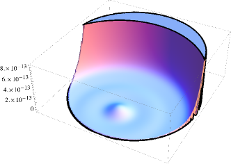
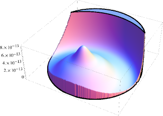
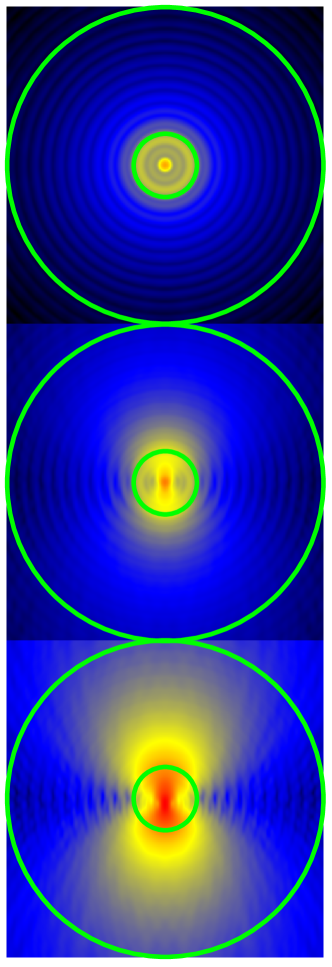
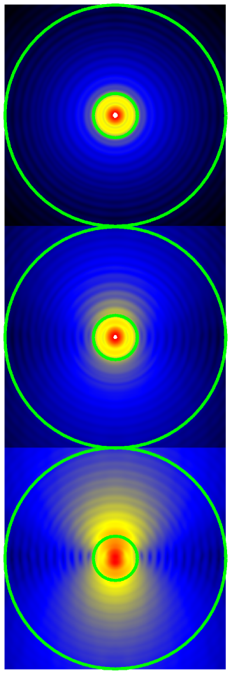
Figure 8: Top curves: pupil plane intensities for an offset of 1 m for $\lambda\in$ (380,750) nm. Density curves below represent the focal plane intensities (log scale) for telescope positions: on-axis (upper curves) and offsets of 50 cm (intermediate curves) and 1 m (lower curves). Left: aperture optimization, right: focal plane optimization.

Figure 9: Average residual light level $\gamma$ for the focal plane (a) and pupil plane (b) optimization, as a function of the telescope offset in centimeters for $\lambda\in$ (380,750) nm. The average is computed over the region from 0.1 to 0.5 arcsec delimited in Fig. 8 by two circles.

5 Conclusion

We addressed the problem of optimizing of the shape of a circularly symmetric apodized occulter. To this end, we proposed a general expression for the attenuation function, as a weighted sum of basis functions. We expressed the optimization problem as the minimization of the flux, first in the pupil plane, as is commonly done in the literature, and then in the focal plane of a 4.m diameter telescope, for a region between 0.1 to 0.5 arcsec in which the exoplanet is supposed to be observed.

Numerical experiments show that the focal plane optimization leads to a better attenuation of the starlight than the pupil plane optimization. One interesting result is that while the focal plane optimization leads to a strong flux in the pupil plane, most of this light is concentrated in the area behind the occulter in the focal plane, which is not a problem for a perfect telescope. Finally, the robustness of our approach to lateral misalignment of the occulter was investigated and showed that the focal plane optimization also yields a better robustness.

As already indicated, the optimization study was made for a 4m telescope assumed to be at its on-axis position. A simple procedure to make the experience less sensitive to defect position would be to perform the optimization for a larger aperture than is actually used. A better procedure would be to estimate the statistics of pointing errors and include them in the optimization procedure. Then a better tolerance to pointing errors would be obtained, probably at the expenses of a tolerable loss in the starlight rejection. Nevertheless, our analysis showed that telescope offsets of a few decimeters will not strongly reduce the efficiency of the occulter.

This conclusion was obtained for the condition that the telescope has a perfectly circular aperture and another study is required to model a telescope with central obscuration. Moreover, it would be interesting to study the effect of a a more realistic telescope with small defaults of phase and amplitude. Deviations from this perfection could lead to somewhat different results, but the exigency of quality is limited to a maximum of 0.5 arcsec, or about twenty Airy rings for a 4m diameter telescope. Finally, with the knowledge of the exact PSF of the telescope, one can readily adapt our optimization approach. A comparison of pupil vs focal optimization for the maximum-magnitude minimization as in Kasdin et al. (2013) would also be interesting.

Appendix A Quality test of the numerical computation using an analytical expression for a sharp-edged circular occulter

Aime (2013) has shown, using an approach similar to Born & Wolf (1999), that an analytic expression using Lommel series could be derived for the Fresnel diffraction of a sharp circular occulter of the form $f(r)=f_{\bullet}(r,\Omega)=\Pi(r/\Omega)$, defining here $\Pi(r)$ as the function equal to 1 for $|r|\leq 1$ and 0 otherwise. At the wavelength $\lambda$, the complex amplitude $\psi_{\bullet}(r,\Omega)$ of the wave at the distance $z$ for

(i) inside the geometrical umbra ($r<\Omega$) and

(ii) outside ($r>\Omega$),

can be written using two series:

$$\begin{split}\psi_{\bullet}(r,\Omega)=&\\ (i)\;\;&\tau(r)\;\tau(\Omega)\;\sum_{n=0}^{\infty}(-i)^{n}(\frac{r}{\Omega})^{n}J_{n}(\frac{2\pi\Omega r}{\lambda z})\\ (ii)\;&1-\tau(r)\;\tau(\Omega)\;\sum_{n=1}^{\infty}(-i)^{n}(\frac{\Omega}{r})^{n}J_{n}(\frac{2\pi\Omega r}{\lambda z}).\end{split}$$ (14)

At $r=\Omega$, both series converge to the same value given by

$$\psi_{\bullet}(\Omega,\Omega)=\frac{1}{2}(1+\exp(i\frac{2\pi\Omega^{2}}{\lambda z})J_{0}(\frac{2\pi\Omega^{2}}{\lambda z})).$$ (15)

These series are alternative series for the real and imaginary terms, and according to the Leibniz estimate, an upper bound of the error for the sum limited to $n=N$ terms is given by the absolute value of the $N+1$ term. The convergence is easy when $r/\Omega$ is smaller than 1, for the first sum for $r<\Omega$ inside the geometrical umbra, or the inverse outside. The main error occurs near the transition zone $r=\Omega$.

In Fig.10 we compare the analytical and numerical results for an example of a circular occulter of 50 m diameter set at 80 000 km, and for a wavelength of 550 nm. The Lommel series were computed for 100 terms, and there is no difference between the two methods. Results were drawn for the real, imaginary, modulus, and unwrapped phase of the Fresnel diffraction. Note that this is just an example, in particular, the real and imaginary part of the diffraction pattern are highly sensitive to a small variation of any of the parameters. The modulus of the intensity pattern clearly shows the visible Poisson spot at the center of the pattern. The unwrapped phase presents a strong phase variation in the center of the umbra and a quieter structure outside the geometric umbra, that is for a region utilized by the telescope for the planet observation. The consistency between the two analytic and numerical results is recognized here as a proof of the quality of the numerical calculation.

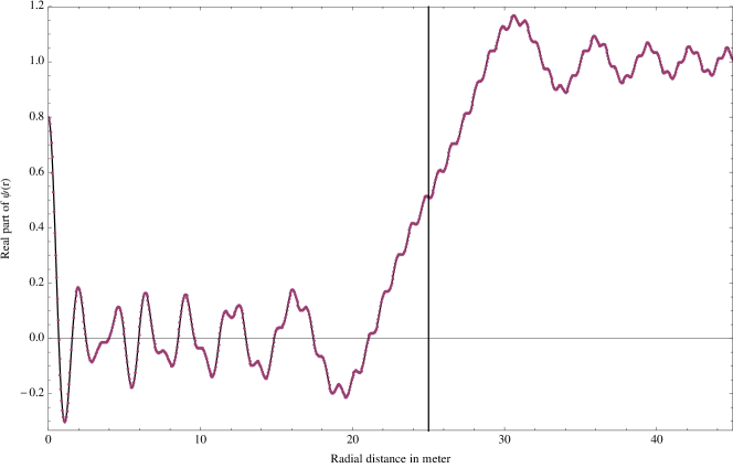
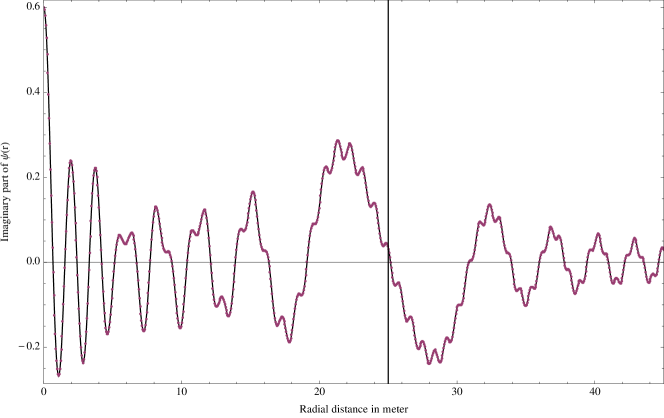
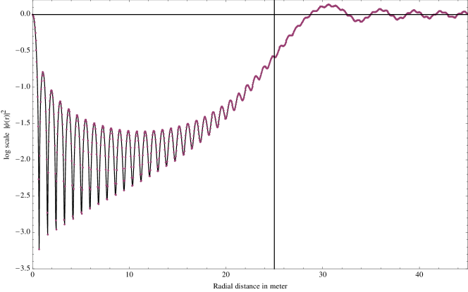
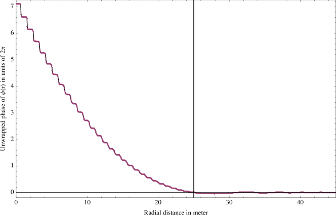
Figure 10: From top to bottom: real, imaginary, squared modulus and unwrapped phase of $\psi(r)$ for a circular occulter of radius $\Omega=25$ m (the vertical line) at $z=80000$ km for $\lambda=0.55\mu$ m. The continuous line represents the Lommel series, dots are the result of a direct numerical computation of Eq. 1 using NIntegrate of Mathematica

Appendix B Numerical calculation of linearly apodized basis functions $f_{k}(r)$

As indicated in the body of the paper, we tried several forms for the set of apodized basis functions $f_{k}(r)$, and decided to use the simple trapezoidal functions described in the body of the paper because they affect the final solution the least. We did not succeed in deriving an analytic form for the Fresnel diffraction of these functions, but comforted by the results obtained on the Fresnel diffraction of $\Pi(r/\Omega)$, we used the direct numerical calculation of Mathematica.

We recall that these functions are linearly apodized disks of radii varying from 10 m to 25 m in steps of 5 cm, the apodization applies for 5 cm at the edge. The resulting $\psi_{k}(r)$ are very similar to those obtained for the functions $\Pi(r/\Omega)$. Differences between moduli are lower than $1\%$, as shown in Fig. 11 for two extreme cases, but essential to obtain proper results on diffraction patterns. In Fig. 12 we focus on the central part of the diffraction pattern, for $r\leq 2$ m. Curves are drawn for a raw and linearly apodized occulter of 10 m and 10.05 m.

Figure 11: Differences of moduli of Fresnel diffractions for raw and linearly apodized functions for $\Omega$ values of 10 m (thick curve) and 10 m (thin curve).

Figure 12: Representation for $r$ between 0 and 2 m of the moduli of $\psi_{k}(r)$ of linearly apodized occulters of radii 10 m and 10.05 m (a). The two curves are almost over imposed, and curve (b) represents 100 times their differences.