Symmetric ribbon disks

Abstract

We study the ribbon disks that arise from a symmetric union presentation of a ribbon knot. A natural notion of symmetric ribbon number $r_{S}(K)$ is introduced and compared with the classical ribbon number $r(K)$. We show that the difference $r_{S}(K)-r(K)$ can be arbitrarily large by constructing an infinite family of ribbon knots $K_{n}$ such that $r(K_{n})=2$ and $r_{S}(K_{n})>n$. The proof is based on a particularly simple description of symmetric unions in terms of certain band diagrams which leads to an upper bound for the Heegaard genus of their branched double covers.

1 Introduction

Symmetric unions (see Section 2 for definitions) were first introduced by Kinoshita and Terasaka in [6]. Christoph Lamm began a systematic investigation in [7]. One of the main questions which motivate the study of symmetric unions is the following.

Question 1.

Does every ribbon knot admit a symmetric union presentation?

In [7] it is shown that all ribbon knots up to ten crossings have a symmetric union presentation. In [8] the result is extended to all 2-bridge ribbon knots. In [2] Eisermann and Lamm introduced a natural notion of symmetric equivalence between symmetric union presentations providing a list of symmetric Reidemeister-like moves. This notion is further investigated in [3] where a refined version of the Jones polynomial is adapted to this setting.

One way to measure the complexity of a given ribbon knot $K$ is to consider its ribbon number $r(K)$ which is the minimal number of ribbon singularities among all ribbon disks spanning $K$. Every symmetric union presentation has an obvious symmetric ribbon disk associated with it, therefore it makes sense to define the symmetric ribbon number $r_{S}(K)$ of a given ribbon knot $K$. Set $r_{S}(K)=\infty$ if $K$ does not admit a symmetric union presentation. Keeping Question 1 in mind it is natural to compare the ribbon number and its symmetric version for a given knot. It turns out that the complexity of a symmetric union presentation (as measured by the symmetric ribbon number) can be arbitrarly large even for knots with $r(K)=2$.

Theorem 1.

For each positive integer $n$ there exists a ribbon knot $K_{n}$ such that $r(K_{n})=2$ and $r_{S}(K_{n})>n$.

We do not know if any of the ribbon knots in the family $\{K_{n}\}$ admits a symmetric union presentation and we suspect that many of them do not. These knots are constructed as satellites of the simplest non trivial ribbon knot, i.e. the connected sum of a trefoil knot with its mirror image. The proof is based on the fact that for any ribbon knot $r_{s}(K)$ gives un upper bound for the Heegaard genus of the branched double cover along $K$. We also show that there is a similar inequality involving the free genus of $K$.

In Section 2 we briefly review basic properties of symmetric unions and we establish the inequalities we need. In Section 3 we introduce the family $\{K_{n}\}$ and give an estimate for the Heegaard genus of their branched double covers which is needed to complete the proof of Theorem 1.

2 Symmetric Unions, Branched Double Covers and the Free Genus

A symmetric union presentation of a knot is a diagram obtained in the following way. We start with the symmetric diagram of a connected sum between a knot and its mirror image, and then we add crossings on the axis of symmetry. See Figure 1 for some examples taken from [7]. See also [7] for a formal definition.

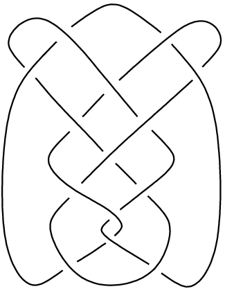
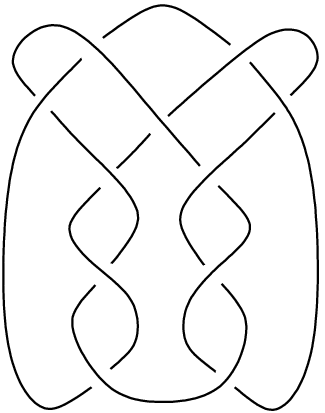
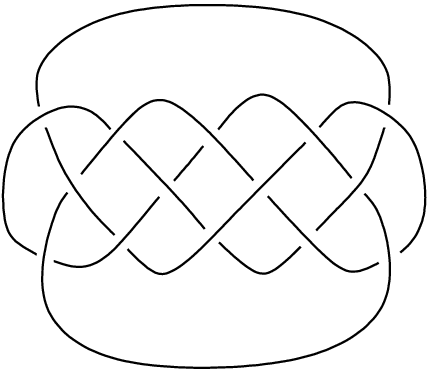
Figure 1: Symmetric union presentations for the knots $9_{41}$, $10_{22}$ and $10_{123}$.

The obvious reflection will fix the knot except near crossings on the axis which are necessarly reversed. More generally one can talk about symmetric diagrams, these will represents links that bounds ribbon surfaces consisting of annuli, Mobius strips and disks. Each symmetric union diagram describes an obvious ribbon disk spanning the given knot, see Figure 2 for an example.

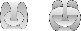
Figure 2: On the left: a symmetric link diagram bounding a ribbon surface consisting of a disk and an annulus. On the right: a symmetric union diagram and the corresponding symmetric ribbon disk.

This disk is obtained by joining symmetric points with a straight line (see [2]). We call such disks symmetric ribbon disks. Recall from [1] that every ribbon disk (and more generally every ribbon surface) in $S^{3}$ admit a diagram, called a band diagram, made up from the elementary pieces shown in Figure 3.

Figure 3: Elementary pieces of band diagrams

The second picture represents a junction. The third picture represents a band crossing and the fourth one a ribbon singularity. Our first observation is that symmetric ribbon disks admit a nice combinatorial characterization in terms of band diagrams.

Proposition 1.

Every symmetric ribbon disk admits a band diagram without any band crossings nor junctions. Conversely, every ribbon disk that has a band diagram without band crossings or junctions is a symmetric ribbon disk.

Proof.

First note that each crossing on the axis corresponds to a half twist of a band which is a portion of the symmetric ribbon disk. As a first step we momentarily remove all these twists by smoothing crossings on the axis as shown in Figure 4.

Figure 4: How to smooth crossings on the axis so that they correspond to the removal of half twists in the symmetric ribbon disk.

Recall that the disk is obtained by joining symmetric points with a straight line orthogonal to the symmetry plane. It follows that the projection of the disk onto the symmetry plane consists of an arc with selfintersections (double points). For example by projecting the symmetric ribbon disk in Figure 2 on its symmetry plane we get the curve in Figure 5.

Figure 5: A selfintersecting curve resulting from the projection of a symmetric ribbon disk onto its symmetry plane.

Each smooth point on this curve corresponds to a properly embedded interval in the ribbon disk while double points correspond to ribbon singularities. The desired band diagram may be obtained by slightly perturbing this projection as follows. First we modify the projection in a neighbourhood of each double point as shown in Figure 6.

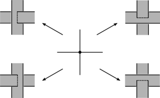
Figure 6: How to perturb the projection near a double point.

The perturbation is obtained by rotating each band on its core, this may be done in two different ways which correspond to the two rows in Figure 6. Now we slightly perturb the rest of the projection which appears as a collection of arcs. Each arc will appear as a band after a rotation on its core. Finally note that all these local choices for the rotation of bands can produce band twists. Specifically twists will arise each time two adiacent bands are rotated in opposite directions.

Now the original crossings on the axis can be restored. Each crossing on the axis correspond to a half twist of a band of the ribbon disk. This band may be located in the projection we just obtained and the half twist can be reinserted. The band diagram obtained in this way has no band crossings and no junctions.

Conversely suppose we are given a band diagram of a ribbon disk without band crossings and without junctions. Near each ribbon singularity we may change the projection to obtain a pair of arcs intersecting trasversely in a single point (see Figure 6). We may do the same for the bands connecting these ribbon singularities. Each band will look like an arc outside small regions corresponding to band twists. Near each ribbon singularity we may choose a plane parallel to the projection plane that cuts each band along its core. We may assume that all these planes coincide because all ribbon singularities are connected by band in planar fashion. We may also assume that the plane cuts each band connecting two ribbon singularities along its core (except near band twists). All these adjustments may be carried out without altering our projection. Note that the reflection across this plane fixes the knot except near the band twists. A symmetric union diagram can be obtained by projecting the knot onto any plane orthogonal to symmetry plane.

∎

Remark 1.

The band diagram obtained in the above proof has the same number of ribbon singularities as the original symmetric ribbon disk.

Remark 2.

Proposition 1 holds in the more general context of symmetric diagrams. Every symmetric link bounds a ribbon surface consisting of disks, annuli and Mobius bands. A suitable projection can be chosen so that this surface can be described via a band diagram without band crossings and without junctions. The proof is the same as that of Proposition 1.

Before we explore some consequences of Proposition 1 we introduce some notation. Given a knot $K$ we indicate by $g_{F}(K)$ the free genus of $K$, i.e. the minimal genus among all Seifert surfaces spanning $K$ whose complement have free fundamental group (these are sometimes called regular Seifert surfaces). We denote by $\Sigma(K)$ the branched double cover of $S^{3}$ branched along $K$. Finally for any closed orientable 3-manifold $Y$ we denote by $g_{H}(Y)$ its Heegaard genus.

Proposition 2.

Let $K$ be a ribbon knot, and let $D$ be a symmetric ribbon disk which minimizes the number of ribbon singularities.

1. $S^{3}\setminus D$ has free fundamental group and its rank equals $r_{S}(K)$

2. $r_{S}(K)\geq\frac{1}{4}(g_{H}(\Sigma(K))+1)$

3. $r_{S}(K)\geq g_{F}(K)$

Proof.

The first assertion is clear from the proof of Proposition 1 and Remark 1.

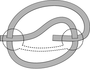
Figure 7: A decomposition of $(S^{3},K)$ that lifts to a Heegaard decomposition of $\Sigma(K)$.

Choose a band diagram for $D$ without band crossings and without junctions. We can enclose each ribbon singularity in a ball whose boundary intersects the knot in exactly eight points. Now we can connect these balls with unknotted tubes disjoint from $D$, in this way we obtain a decomposition of $S^{3}$ into two balls $B_{1}$ and $B_{2}$. Each pair $(B_{i},B_{i}\cap K)$ is homeomorphic to the standard ball containing a trivial braid, therefore this decomposition lifts to a Heegaard decomposition for $\Sigma(K)$ of genus $3r_{S}(K)$ (see Figure 7 for an example). The inequality follows.

Let us fix again a band diagram for $D$ without band crossings and without junctions and an orientation for $K$. Near each ribbon singularity there are four possible oriented configurations as shown in Figure 8.

Figure 8: The four possible oriented configurations of a ribbon singularity

By flipping the horizontal band if necessary we may assume that only the first two cases occur. Now assume, momentarly, that there are no band twists in our diagram. In this situation the Seifert algorithm will produce a regular Seifert surface $S$ whose genus is precisely $r_{S}(K)$. To see this note that near each ribbon singularity the oriented resolution gives four arcs corresponding to the four bands connected to the ribbon singularity. All but two of the Seifert circles will appear as an arc on two ribbon singularities (once these are appropriately resolved). Therefore the number of Seifert circles of $S$ is $2r_{S}(K)+1$. This means that the Euler characteristic is $\chi(S)=2r_{S}(K)+1-4r_{S}(K)=1-2r_{S}(K)$ from which we obtain $g(S)=r_{S}(K)$. It is easy to check that band twists do not alter the computation we made above because they do not change the Seifert graph associated to $S$. ∎

3 The Family $\{K_{n}\}$

In this section we will construct an infinite family of ribbon knots $\{K_{n}\}$ such that $r(K_{n})=2$ and $g_{H}(\Sigma(K_{n}))\geq n$. This fact together with the second assertion of Proposition 2 will conclude the proof of Theorem 1. The idea is to start with a very simple ribbon knot and then replace a piece of unknotted band with a knotted one, this operation will change the knot and its ribbon disk without changing its ribbon number. See Figure 10 for an example.

First we recall some basic terminology and facts from [9]. By a tangle we mean a pair $(B,t)$ where $B$ is a 3-ball and $t$ is a pair of properly embedded arcs in $B$. Two tangles $(B,t),(B^{\prime},t^{\prime})$ are equivalent if there is an homeomorphism of pairs from $(B,t)$ to $(B^{\prime},t^{\prime})$. A tangle is said to be untangled is it is equivalent to the trivial tangle (these are usually called rational tangles). A tangle is locally unknotted if every 2-sphere which meets $t$ transversely in two points bounds a ball which meets $t$ in an unknotted arc. Finally a locally unknotted tangle which is not untangled is said to be prime. Given two tangles $(B,t)$, $(B^{\prime},t^{\prime})$ and a homeomorphism $\varphi:(\partial B,\partial t)\rightarrow(\partial B^{\prime},\partial t^{\prime})$ a link can be obtained by identifying the boundaries of the two tangles via $\varphi$. We say that such a link is obtained as the sum of the tangles $(B,t)$ and $(B^{\prime},t^{\prime})$. We will also need the notion of partial sum between tangles. This operation consists in identifying a $(\textrm{disk},\textrm{pair of points})$ pair in the boundary of a tangle with a similar pair in the boundary of another tangle so that the result is still a tangle.

Theorem 2.

[9] Let $(B,t)$ be a prime tangle. Its branched double cover $Y$ is irreducible and its boundary $\partial Y$ is incompressible.

We recall from [4] the following theorem.

Theorem 3.

There exists a constant $C_{g}$ such that for every closed, orientable and irreducible 3-manifold $M$ of Heegaard genus $g$ and every collection $T_{1},\dots,T_{k}$, $k>C_{g}$ of disjoint incompressible tori in $M$ at least two of them $T_{i}$ and $T_{j}$ are parallel.

Let $T_{1}$ and $T_{2}$ be the tangles depicted in Figure 9. Let $K_{n}$ be the knot obtained as an iterated partial sum of the tangle $T_{1}$ and $n$ copies of the tangle $T_{2}$ as depicted in Figure 10.

As is clear from the picture each $K_{n}$ is a nontrivial knot bounding a ribbon disk with two ribbon singularities. Moreover it is easy to show that every ribbon disk with less than two ribbon singularities is bounded by the trivial knot (for these and other considerations on the ribbon number see for instance [10]). We conclude that $r(K_{n})=2$ for each $n>0$.

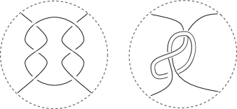
Figure 9: Two prime tangles.

Proposition 3.

For each positive integer $k$ there exists $n_{k}$ such that

$$g_{H}(\Sigma(K_{n_{k}}))>k$$

Proof.

It is shown in [9] that the tangles $T_{1}$ and $T_{2}$ are prime and that summing prime tangles gives prime knots. By [5] a link in $S^{3}$ is prime if and only if its branched double cover is irreducible. It follows that each $\Sigma(K_{n})$ is an irreducible 3-manifold.

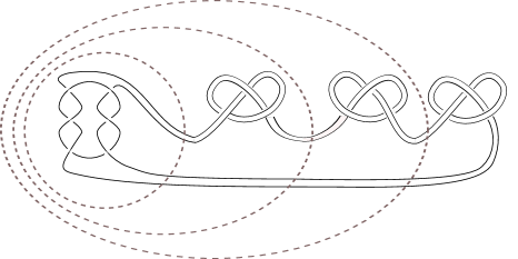
Figure 10: The knot $K_{3}$. Each sphere lifts to an incompressible torus in the branched double cover

By Theorem 2 each sphere depicted in Figure 10 lifts to an incompressible torus in $\Sigma(K_{n})$. We have $n$ disjoint incompressible tori, in order to apply Theorem 3 we only need to show that these tori are pairwise non parallel. Choose a pair of tori and assume by contradiction that they are parallel. By Dehn filling each boundary component we would obtain a Lens space. This filling may be chosen so that it corresponds to the sum of trivial tangles in $S^{3}$ which gives a cable of a connected sum of trefoil knots. Since this knot is not a 2-bridge knot its branched double cover cannot be a Lens space. ∎

References

- [1] M. Eisermann, The Jones polynomial of ribbon links, Geometry and Topology 13 (2009) 623-660
- [2] M. Eisermann, C. Lamm, Equivalence of symmetric union diagrams, J. Knot Theory Ramifications 16, 879 (2007) 879-898
- [3] M. Eisermann, C. Lamm, A refined Jones polynomial for symmetric unions, Osaka J. math. 48, 2011 333-370
- [4] M. Eudave-Munoz, J. Shor, A universal bound for surfaces in 3-manifolds with a given Heegaard genus, Alg. Geom. Top. 1 (2001) 31-37
- [5] P. K. Kim, J. L. Tollefson, Splitting the P.L. involutions of nonprime 3-manifolds, Michigan Math. J. 27, 1980 259-274
- [6] S. Kinoshita, H. Terasaka, On unions of knots, Osaka J. Math. 9, 1957 131-153
- [7] C. Lamm, Symmetric unions and ribbon knots, Osaka J. Math. 37, (2000) 537-550
- [8] C. Lamm, Symmetric union presentations for 2-bridge ribbon knots, http://arxiv.org/abs/math/0602395
- [9] W. B. Lickorish, Prime knots and tangles, Trans. Amer. Math. Soc. 267 (1981) 321-332
- [10] Y. Mizuma, An estimate of the ribbon number by the Jones polynomial, Osaka J. Math. (2006) 365-369