Modeling radio communication blackout and blackout mitigation in hypersonic vehicles

Abstract

A procedure for the modeling and analysis of radio communication blackout of hypersonic vehicles is presented. The weakly ionized plasma generated around the surface of a hypersonic reentry vehicle is simulated using full Navier-Stokes equations in multi-species single fluid form. A seven species air chemistry model is used to compute the individual species densities in air including ionization - plasma densities are compared with experiment. The electromagnetic wave’s interaction with the plasma layer is modeled using multi-fluid equations for fluid transport and full Maxwell’s equations for the electromagnetic fields. The multi-fluid solver is verified for a whistler wave propagating through a slab. First principles radio communication blackout over a hypersonic vehicle is demonstrated along with a simple blackout mitigation scheme using a magnetic window.

Nomenclature

A	=	amplitude of oscillation
$\vec{B}$	=	magnetic field, T
$\vec{B}$0	=	background static magnetic field, T
c	=	speed of light, m/s
cp	=	specific heat at constant pressure, J/kg K
cv	=	specific heat at constant volume, J/kg K
$\vec{E}$	=	electric field, V/m
e	=	total (internal+kinetic+chemical) energy of the fluid , J/m3
	=	electron
f	=	number of degrees of freedom
	=	frequency, Hz
H	=	enthalpy of formation, J/particle
I	=	identity matrix
kT	=	thermal conductivity, W/m K
k	=	wave number
kB	=	Boltzmann constant, J/K
m	=	mass of a unit species, kg
M	=	molecular weight, g/mol
n	=	number density, 1/m3
N	=	number of species or fluids in the system
q	=	charge of a unit species, C
Q	=	internal energy exchange rate per unit volume, W/m3
QEM	=	energy density of the electromagnetic wave, J/m3
R	=	gas constant, J/kg K
$\vec{R}$	=	momentum exchange rate per unit volume, N/m3
t	=	time, s
T	=	temperature, K
$\vec{u}$	=	velocity, m/s

$\gamma$	=	gas constant (cp/cv)
$\mu$	=	dynamic viscosity, N s/m2
	=	reduced mass, kg
$\rho$	=	density, kg/m3
$\tau$	=	stress tensor, N/m2
$\sigma$	=	collision diameter, m
$\epsilon$0	=	permittivity of free space, F/m
$\zeta$	=	collision time, s
$\Omega$	=	collision integral
$\Omega_{ce}$	=	electron cyclotron frequency, radians/s
$\Omega_{ci}$	=	ion cyclotron frequency, radians/s
$\Omega_{pe}$	=	electron plasma frequency, radians/s
$\Omega_{pi}$	=	ion plasma frequency, radians/s
Subscripts
$\alpha$	=	index of fluids
e	=	electron
i	=	index of species or fluids
	=	ion
Supercripts
T	=	transpose

I Introduction

Hypersonic vehicles are subjected to severe aerothermal heating due to the formation of shock waves in front of the vehicle. Flow Mach numbers exceeding four are classified as hypersonicbertin1994hypersonic . The shock wave converts the kinetic energy to internal energy and thereby increases the fluid temperatures significantly. The temperatures quite often exceed the dissociation and ionization limits of the flow species and results in the formation of a weakly ionized plasma layer around the vehicle. The electrons in the plasma layer may interrupt the propagation of radio frequency electromagnetic waves, if the plasma electron oscillation frequency exceeds that of the electromagnetic wave frequency. This phenomenon is commonly called radio communication blackout. For instance, a 1.6 GHz radio wave will be interrupted by a plasma layer of density $3.5\times 10^{16}$ m^-3. Blackout mitigation is an important requirement for the design of hypersonic vehicles, especially for those vehicles in steady state hypersonic flight such as those envisioned by NASA and the US Air Force. A few mitigation mechanisms described in the literature are the magnetic windowhodara1961 ; manning2009analysis ; thoma2009electromagnetic ; starkey2003electromagnetic ; usui2000Computer , electrophilic fluid injectionmeyer2007system , wave frequency modification, aerodynamic shape modification, $E\times B$ driftgillman2010review ; keidar2008electromagnetic , resonant transmissionsternberg2009resonant , time varying magnetic fieldstenzel2013new and electron acoustic wave transmissionmudaliar2012radiation . The magnetic window uses a static magnetic field to convert the free space radio wave to a whistler wave in the plasma.stenzel1976whistler ; usui2000Computer Electrophilic injection uses an electrophilic substance injected into the fluid to decrease the electron density. Wave frequency and aerodynamic shape modification have design limitations so may be impractical in many cases. The $E\times B$ drift accelerates the ions in the layer there by decreasing the plasma density near the antenna. Resonant transmission uses surface wave resonance to enhance transmission through the plasma layer. The time varying magnetic field approach uses the hall effect to expel ions. Electron acoustic wave transmission works by converting the wave into an electron acoustic wave in the plasma layer. Numerical simulations of blackout mitigation techniques are valuable during the design phase of hypersonic vehicles.

Radio communication blackout modeling of aerospace vehicles with full wave electromagnetics has been investigated by several groups with many different codes. Takahashitakahashi2014prediction ; takahashi2014examination used a CFD tool to compute the plasma distribution and then a FDTD solver with a modified permittivity to account for the presence of a plasma. Usui usui2000Computer demonstrated one dimensional PIC simulation of the whistler wave propagation in an assumed dense plasma profile. Thomathoma2009electromagnetic used the high density FDTD PIC code LSP to investigate the magnetic window with a horn antenna surrounded by an assumed plasma distribution. Visbalvisbal2008high used a multi-fluid electromagnetic approach to modeling radio communication blackout on an over-set mesh, without an investigation of steady magnetic field effects. Starkeystarkey2003electromagnetic used one dimensional finite volume inviscid solver to estimate the plasma density on hypersonic vehicles along their trajectories and analyzed the whistler wave propagation using an imposed constant magnetic field.

The present paper shows the combined modeling approach to simulate the blackout mitigation devices and the surrounded reactive flows in complex geometries of realistic hypersonic vehicles. The finite volume simulation model used in the present work simulates the multi-species/fluid flow, reactions, plasma generation, and electromagnetic fields in the fluid without ignoring the plasma waves. RAM C reentry vehicle is used for this demonstration as there is a significant experimental data for comparison.jones1972electrostatic USimloverich2013nautilus ; shashurin2014laboratory ; kundrapu2013modeling , a commercial code developed by Tech-X Corporation for general fluid plasma modeling on unstructured grids, is used for all simulations in this paper. This paper is organized as follows: (1) Modeling and simulation of the multi-species hypersonic flow over the RAM C reentry vehicle to obtain the plasma density distribution (2) Validation of the plasma density distribution with the results from literature (3) Modeling of electromagnetic wave propagation into the plasma and validation with the dispersion relation and (4) Finally, the propagation of plane EM wave on to the vehicle’s surface through the plasma layer using a magnetic window and the whistler wave conversion.

II Mathematical formulation

II.1 Bulk fluid transport

A generalized model for simulating the compressible flow with reacting multi-species is given in this section. The Navier-Stokes equations in conservative form Eqs. (1)–(3) are used for the conservation of fluid mass, momentum, and total energy respectively. The total energy $e$ in Eq. (3) is the sum of internal energy, kinetic energy and chemical energy of the fluid. The upper limit $N$ in the summation of Eqs. (4) and (7) is the total number of species in the system. The fluid is assumed to be Newtonian and obeys the Stoke’s hypothesis of zero bulk viscosity. Further, the fluid obeys the ideal gas law for equation of state.

$$\frac{\partial\rho}{\partial t}+\nabla\cdot\left(\rho\vec{u}\right)=0$$ (1)

$$\frac{\partial\left(\rho\vec{u}\right)}{\partial t}+\nabla\cdot\left(\rho\vec{u}\vec{u}+pI\right)=\nabla\cdot\mathbf{\tau}$$ (2)

$$\frac{\partial\left(e\right)}{\partial t}+\nabla\cdot\left(\vec{u}\left(e+p\right)\right)=\nabla\cdot\left(\tau\cdot\vec{u}\right)+\nabla\cdot\left(k_{T}\nabla T\right)$$ (3)

where,

$$\rho=\sum\limits_{i}^{N}{n_{i}m_{i}}$$ (4)

$$p=\rho RT$$ (5)

$$\tau=-\frac{2}{3}\mu\left(\nabla\cdot\vec{u}\right)I+\mu\left(\nabla\vec{u}+\left(\nabla\vec{u}\right)^{T}\right)$$ (6)

$$e=\frac{p}{\gamma-1}+\frac{1}{2}\rho\vec{u}\cdot\vec{u}+\sum\limits_{i}^{N}{n_{i}H_{i}}$$ (7)

and

$$\gamma=\frac{c_{p}}{c_{p}-R}$$ (8)

II.2 Species transport

The mass conservation of the individual species in the bulk fluid is satisfied separately for each of the species using Eq. (9). The velocity $\vec{u}$ is the same as that of the bulk fluid. The right hand side of Eq. (9) represents the rate of change of species density due to the chemical reactions. In a given chemical reaction, the rates of change of species density are obtained using the forward and backward reaction rates and the existing number densities of the reactants and products. The rates of change of a species $i$ in all of the reactions are added to get $s_{i}$.

$$\frac{\partial n_{i}}{\partial t}+\nabla\cdot\left(\vec{u}n_{i}\right)=s_{i}$$ (9)

II.3 Material properties

The properties viscosity, thermal conductivity and specific heat of the individual species are obtained from the kinetic theory of gases as given by the Eqs. (11)–(13). The fluid thermal conductivity $k$ and viscosity $\mu$ in Eqs. (1)–(3) are obtained using mole fraction averaging while the specific heat $c_{p}$ is obtained using the mass fraction averaging. The gas constant $R$ is computed using the mole fraction averaged molecular weight.

$${c_{p}}_{i}=\left(\frac{f}{2}+1\right)R_{i}$$ (10)

$$\mu_{i}=\frac{5}{16}\frac{\sqrt{\pi m_{i}k_{B}T}}{\left(\pi\sigma^{2}\Omega\right)}$$ (11)

$$k_{i}=\frac{5}{2}{c_{v}}_{i}\mu_{i}$$ (12)

$${c_{v}}_{i}={c_{p}}_{i}-R_{i}$$ (13)

II.4 Electromagnetic multi-fluid

A multi-fluid model is used for the interaction of a radio wave with the plasma. Maxwell’s equations are used to solve for the evolution of the electric and magnetic fields. Ampere’s law and Faraday’s law are given by Eqs. (14) and (15) respectively. The right hand side of Eq. (14) is the sum of the current densities of the conducting fluids. The upper limit $N$ in the summation is the total number of fluids in the system. The divergence equations (16) and (17) should be satisfied along with the Ampere’s and Faraday’s laws.munz2000athreedimensional

$$\frac{\partial\vec{E}}{\partial t}-c^{2}\nabla\times\vec{B}=-\frac{1}{\epsilon_{0}}\sum\limits_{\alpha}^{N}\frac{q_{\alpha}\rho_{\alpha}\vec{u}_{\alpha}}{m_{\alpha}}$$ (14)

$$\frac{\partial\vec{B}}{\partial t}+\nabla\times\vec{E}=0$$ (15)

$$\nabla\cdot\vec{E}=\frac{1}{\epsilon_{0}}\sum\limits_{\alpha}^{N}\frac{q_{\alpha}\rho_{\alpha}}{m_{\alpha}}$$ (16)

$$\nabla\cdot\vec{B}=0$$ (17)

The transport of the multi-fluid system is modeled using the system of equations Eqs. (18)–(20). Index $\alpha$ is for any fluid. The first term on the RHS of Eq.(19) represents the electric and magnetic Lorentz forces. The third term is the net momentum exchange with the remaining fluids in the system.zhdanov2002transport The first term on the RHS of Eq.(20) is for Joule heating and the fourth and fifth terms are kinetic energy and internal energy exchange terms respectively.zhdanov2002transport The bulk velocity $V$, momentum exchange term $R_{\alpha}$, and the internal energy exchange term $Q_{\alpha}$ are given by Eqs. (21)–(23) respectively.

$$\frac{\partial\rho_{\alpha}}{\partial t}+\nabla\cdot\left(\rho_{\alpha}\vec{u}_{\alpha}\right)=0$$ (18)

$$\frac{\partial\left(\rho_{\alpha}\vec{u}_{\alpha}\right)}{\partial t}+\nabla\cdot\left(\rho_{\alpha}\vec{u}_{\alpha}\vec{u}_{\alpha}+p_{\alpha}I\right)=\frac{\rho_{\alpha}}{m_{\alpha}}q_{\alpha}\left(\vec{E}+\vec{u}_{\alpha}\times\vec{B}\right)+\nabla\cdot\mathbf{\tau}_{\alpha}+\vec{R}_{\alpha}$$ (19)

$$\frac{\partial\left(e_{\alpha}\right)}{\partial t}+\nabla\cdot\left(\vec{u}_{\alpha}\left(e+p_{\alpha}\right)\right)=\frac{\rho_{\alpha}}{m_{\alpha}}q_{\alpha}\vec{u}_{\alpha}\cdot\vec{E}+\nabla\cdot\left(\tau_{\alpha}\cdot\vec{u}_{\alpha}\right)+\nabla\cdot\left(k_{\alpha}\nabla T_{\alpha}\right)+\vec{V}_{\alpha}\cdot\vec{R}_{\alpha}+Q_{\alpha}$$ (20)

where,

$$\vec{V}=\left(\sum\limits_{i}^{N}\rho_{i}\vec{u}_{i}\right)/\sum\limits_{i}\rho_{i}$$ (21)

$$\vec{R}_{\alpha}=-\sum\limits_{i\neq\alpha}^{N}\frac{\rho_{\alpha}}{m_{\alpha}}\mu_{\alpha i}\zeta_{\alpha i}^{-1}\left(\vec{u}_{\alpha}-\vec{u}_{i}\right)$$ (22)

and

$$Q_{\alpha}=-\sum\limits_{i\neq\alpha}^{N}3k_{B}\frac{\rho_{\alpha}}{m_{\alpha}}\left[\mu_{\alpha i}/\left(m_{\alpha}+m_{i}\right)\right]\zeta_{\alpha i}^{-1}\left(T_{\alpha}-T_{i}\right)$$ (23)

Importantly, this model describes electromagnetic wave propagation in free space (where the charged species densities are zero) and in a conducting fluid (where the charged species densities are non-zero). In particular it describes reflection of electromagnetic waves off of an over-dense plasma as well as electromagnetic wave propagation in a plasma including the changes caused by external magnetic fields. The model is more complete to that of magnetohydrodynamics (MHD) and can be thought of as MHD without the assumption of quasi-neutrality, without the assumption that the light wave is infinitely fast and by using the full Ohm’s law, (including electron inertia) in the MHD system. Restricting ourselves to two-fluids for the moment (electrons and ions only), 4 parameters that can be derived from this model, will be important in determining the electromagnetic wave propagation characteristics in the plasma. The first is the electron plasma frequency

$$\Omega_{p\,e}=\sqrt{\frac{n_{e}q_{e}^{2}}{m_{e}\epsilon_{0}}}$$ (24)

the second is the electron cyclotron frequency

$$\Omega_{c\,e}=\frac{q_{e}\,B_{0}}{m_{e}}$$ (25)

followed by the ion plasma frequency

$$\Omega_{p\,i}=\sqrt{\frac{n_{i}q_{i}^{2}}{m_{i}\epsilon_{0}}}$$ (26)

and the ion cyclotron frequency

$$\Omega_{c\,i}=\frac{q_{i}\,B_{0}}{m_{i}}$$ (27)

These parameters will be used in the discussion of the whistler wave.

The system of Eqs. (1)–(13) will be used for the simulation of the bulk fluid and species transport on the RAM C, which will be discussed in Sec. III.1. The species density obtained will serve as input to the blackout analysis. The em wave propagation, reflection by the plasma layer, and whistler mode propagation will be simulated using the Eqs. (14)–(23) in Secs. III.2 and IV. It has to be noted here that, only a simplified version of Eqs. (18)–(20) are used for the fluids transport. The plasma frequency time scale is much smaller than the advection, diffusion and collision time scales, and hence these terms can be neglected. A detailed discussion on the frequencies is given in Sec. IV.

II.5 Solution methodology

The equation systems given in Sec. II are solved using a generalized unstructured grid finite volume solver, USimloverich2013nautilus ; shashurin2014laboratory ; kundrapu2013modeling . Though multi-fluid electromagnetic solvers have been developed throughout the years by several researchers shumlak2003approximate ; hakim2006high ; loverich2011 ; kumar2012entropy ; thompson2013fully ; johnson2013gaussian ; shumlak2013high ; srinivasan2011numerical , the present solver is the first solver using an unstructured formulation and running on an unstructured gridloverich2013nautilus as prior codes were based on multi-block logically Cartesian grids. The flux reconstruction on the cell faces is carried out using second order accurate Monotonic Upstream-Centered Scheme for Conservation Laws (MUSCL)vanLeer1979towards . The right and left fluxes on the cell faces were obtained by extrapolating the cell centered gradient of the conserved variable. The spurious oscillations that may arise due to the flux reconstruction are limited using flux limiters such as Van-Leer limiter.vanLeer1979towards The cell centered gradient is computed using the weighted least squares method. A second degree polynomial is considered in this work. The actual flux on the cell face is then obtained using an approximate Riemann flux. In this work HLLE approximate Riemann fluxeinfeldt1988godunov is considered for the fluid equations while full wave flux is chosen for the Maxwell’s equations. The diffusion fluxes are evaluated by computing the least squares gradient on the cell faces and then performing a surface integral according to the Gauss divergence theorem. The bulk fluid velocity is used to advect the species in in Eq. (9). The same flux scheme is used as that of the bulk fluid. The species density sources due to chemical reactions are integrated separately using the Boost ODE integratorahnert2011odeint . The left and right hand side of the Eqs. (1)–(9), (14), and (15) are evaluated separately and added together and then integrated in time using Runge-Kutta method. A third order RK integration scheme is used. Operator splitting is used for the reaction terms and super time stepping for the diffusion terms.

III Validation of the results

III.1 Reactive flow simulation

The simulation is performed for a velocity of 7650 $m/s$, density 2.816$\times 10^{-4}$ $kg/m^{3}$ and temperature 244.3 K. These values correspond to an altitude of 61 $km$. The air species $N_{2}$, $O_{2}$, $N$, $O$, $NO$, $NO^{+}$, and $e$ (electron) are considered for the reaction chemistry and the reaction rates are considered from the Ref. josyula2003governing . The unstructured grid used for the simulation is shown in Fig. (1). The geometry of RAM C vehicle is available in Ref. jones1972electrostatic . RAM C is a blunt cone ballistic body with a nose cap radius of 15.24 cm, half angle $9^{\circ}$, and a length of 1.29 m. The probes mounted on the surface are not modeled in this work. Cubit blacker1994cubit grid generation software is used for the grid generation. The contour flood represents the area of cells in $m^{2}$. The average edge lengths vary from around 0.5 $mm$ at the nose cap region to 1 $mm$ on the lateral surface.

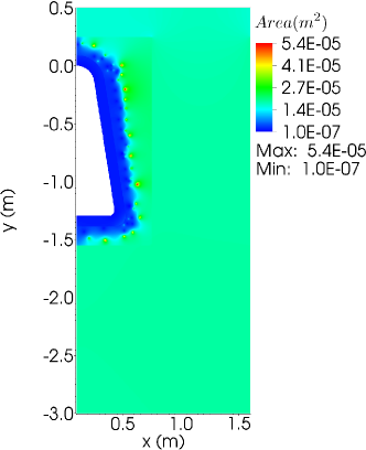
Figure 1: The unstructured grid used for the simulation. The contour flood represents the cell area.

Flow enters the domain from the top boundary of Fig. 1. An axisymmetric boundary condition is imposed on the axis (left boundary). On that wall, a standard no slip and radiation equilibrium temperature are imposed. Outflow boundary conditions are used on the remaining boundaries. The temperature and electron density distributions are shown in Fig. 2. The species are transported with the same advection velocity of bulk fluid. The species densities at the top boundary are equal to their free stream densities and the gradient of species density is zero on the remaining boundaries. The peak values of average temperature and the electron density are 21860 K and $1.18\times 10^{20}$ m^-3 respectively existing in the stagnation region. Figure 3 shows the comparison of the surface and peak electron densities in the plasma layer with the reflectometer measurements presented in Ref. jones1972electrostatic . The measurements represent the time averaged values of the electron density measured using 15 reflectometers of four different frequencies placed at four stations on the wall of RAM C. The cut-off densities associated with the four frequencies are $1.52\times 10^{19}$,$1.25\times 10^{18}$,$1.37\times 10^{17}$, and $1.54\times 10^{16}$ m^-3 respectively.grantham1970flight The first station is located at 0.0457 m from the nosecap tip. The remaining three stations locations along with the measured peak densities are shown by squares in the figure. The dashed curve represents the curve fit of the measured data points. The bottom most curve is the surface density distribution while the top most curve is the peak density of electrons in the plasma layer of Fig.2. The peak values of the simulation are about three times the values from the measurements. Inclusion of radiation losses from the plasma and the diffusion of electrons in the simulation could decrease the density to some extent. Moreover, the comparison shows a good agreement in terms of the trend and in the design point view, the higher values of the simulation to this extent are acceptable in terms of the factor of safety. The wall densities are well below the peak values for the simple reason that the wall temperature is much below the boundary layer temperature.

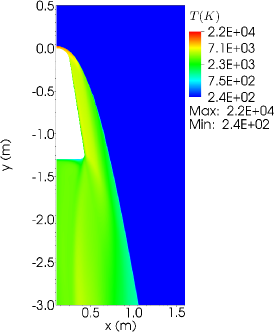
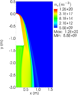
Figure 2: Flow parameters on RAM C. 2 Temperature distribution and 2 electron number density distribution.

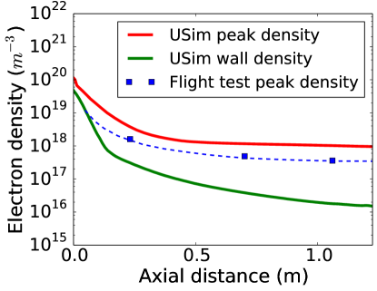
Figure 3: Validation of the electron density in the plasma layer of RAM C. The top and bottom curves are peak density and surface density respectively. The middle curve is the averaged peak density measurements from Ref.jones1972electrostatic

III.2 Dispersion relation for waves parallel to the magnetic field

The magnetic window approach to radio communication blackout mitigation takes advantages of special properties of electromagnetic wave propagation in plasmas in the presence of a magnetic field. A derivation of the whistler wave (as well as many other plasma waves) can be found in many plasma physics text books including goldston2000introduction . In the case below, the dispersion relation is derived from the two-fluid electromagnetic plasma model and written in terms of plasma parameters, $\Omega_{c\,e}$,$\Omega_{c\,i}$,$\Omega_{p\,e}$,$\Omega_{p\,i}$ and the speed of light $c$, the results are given as follows.

The R-Mode dispersion relation is given by

$$k^{2}=\frac{w^{2}\left(w^{2}+w(\Omega_{ci}-\Omega_{ce})-\Omega_{ce}\Omega_{ci}-\Omega_{pe}^{2}-\Omega_{pi}^{2}\right)}{c^{2}(w-\Omega_{ce})(w+\Omega_{ci})}$$ (28)

after ignoring the ion motion, the R-Mode dispersion relation becomes

$$k^{2}=\frac{w\left(w^{2}-w\Omega_{ce}-\Omega_{pe}^{2}\right)}{c^{2}(w-\Omega_{ce})}$$ (29)

.

The L-Mode dispersion relation is given by

$$k^{2}=\frac{w^{2}\left(w^{2}+w(\Omega_{ce}-\Omega_{ci})-\Omega_{ce}\Omega_{ci}-\Omega_{pe}^{2}-\Omega_{pi}^{2}\right)}{c^{2}(w+\Omega_{ce})(w-\Omega_{ci})}$$ (30)

. after ignoring the ion motion, the L-Mode dispersion relation becomes

$$k^{2}=\frac{w\left(w^{2}+w\Omega_{ce}-\Omega_{ce}\Omega_{pe}^{2}\right)}{c^{2}(w+\Omega_{ce})}$$ (31)

Figure 4 shows the frequency vs wave number plotted for the electromagnetic wave in a plasma without a background magnetic field. The vacuum electromagnetic wave is provided for reference. The plasma electromagnetic wave does not propagate below the plasma frequency represented by the horizontal line. This is the reason for radio communication blackout. At all frequencies below the plasma frequency the wave is evanescent. By adding a magnetic field the dispersion relation changes and the wave can propagate through the plasma at frequencies below the electron cyclotron frequency. Figure 5 shows the frequency vs wave number plotted for the R-Mode and L-Mode waves in non-dimensional units in a plasma with a background magnetic field. The R-mode wave has two branches, the lower frequency branch which propagates below the plasma frequency is known as the whistler wave. The whistler wave has a cutoff at the electron cyclotron frequency. In the presence of a magnetic field then it is possible for the electromagnetic wave to penetrate the over-dense plasma. The electron cyclotron frequency must be greater than the signal frequency and this puts a lower bound on the magnetic field strength that should be used. Based on the electromagnetic wave frequency, the background field can be adjusted so that the signal can propagate through the plasma as a whistler wave. This method is termed as the magnetic window in the blackout mitigation studies.

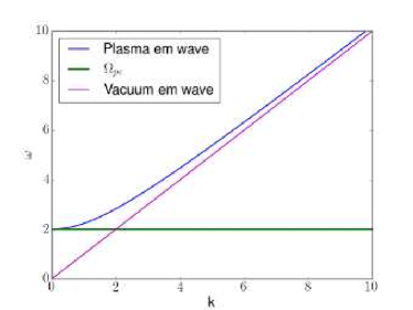
Figure 4: Dispersion graph for electromagnetic waves traveling in a plasma with no background magnetic field, frequency vs wave number in normalized units.

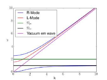
Figure 5: Dispersion graph for electromagnetic waves traveling parallel to the magnetic field, frequency vs wave number in normalized units.

The electromagnetic multi-fluid Eqs. (14)–(17) and (19)–(20) are solved in one-dimension to propagate an EM wave in a neutral fluid and a plasma slab. The advection, diffusion and collision terms are neglected for ion and electron fluids. The simulation results are compared to the analytical calculations of the dispersion relation Eq. (29). Figure 6 shows the EM wave propagation in a neutral fluid. A plane wave is excited from the left boundary with the components E_y = $c\,a_{0}sin(2\pi ft)$ and B_z = E_y/c. The frequency of the wave is 1.6 GHz. Uninterrupted propagation of the wave can be clearly seen. A uniform plasma slab of thickness 0.3 m was then added in the domain at x = -0.15 m. The plasma density is $10^{19}$ m^-3. Since the frequency of the plasma, 28.4 GHz is much greater than the wave frequency, the wave is completely reflected by the plasma. Figure 7 shows the reflection of electric and magnetic fields. The reflected wave components E_y and B_z are shown in Fig. 7 and 7 respectively. The amplitudes of the electric and magnetic fields doubled since a standing wave is formed upon reflection from the plasma slab. The figure also shows the simulation accuracy of the two-fluid solver.jenkins2013time ; merritt2013experimental

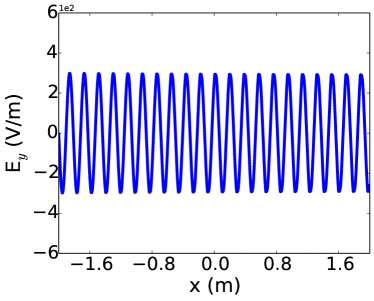
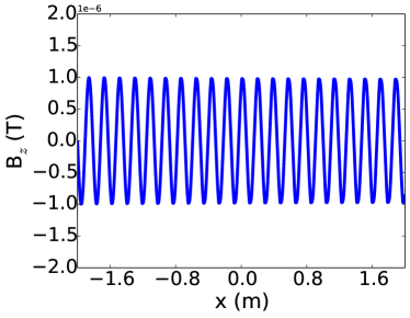
Figure 6: The 6 y component of electric field and the 6 z component of the magnetic field in the EM wave of frequency 1.6 GHz traveling in neutral fluid.

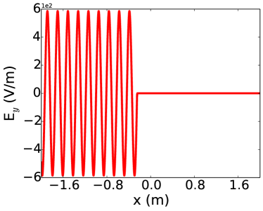
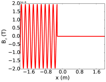
Figure 7: The 7y component of electric field and the 7 z component of the magnetic field of the EM wave of frequency 1.6 GHz traveling in a domain with plasma slab of thickness 0.3 m. The slab starts from x = -0.15 m.

A constant magnetic field of B_0x = 1 T is applied in the domain to create a magnetic window for the propagation of the wave in whistler mode through the plasma. 8 Figure 8 shows the the whistler wave propagation in the plasma slab. Figures 8 and 8 show the wave components E_y and B_z respectively. The whistler wave’s accuracy is compared with the analytical solution obtained from the dispersion theory. The Dispersion relation shows that the wave number of the whistler wave in the plasma slab is 23.89. The Fourier transform of the wave in the spatial domain gives the wave number spectrum. 89 Figure 9 shows the Fourier transform of the wave component E_y of Fig.8. The first peak is located around k = 5.33 and the second peak around k=23.89. The first peak represents the wave in the neutral zone and the second peak corresponds to the wave in the uniform plasma. Note that the amplitude does not match with the values shown in Fig.8 since the exact wavenumbers 5.33 and 23.89 are not resolved by the grid. The current grid represents wave numbers in the multiples of 0.25. The exact peaks are located at 5.5 and 23.75. A more refined grid that represents the wave numbers of interestwould give a matching spectral amplitude to that of the waves in the simulation. Simulations are not performed on a further refined grid, since the wave number peaks are predicted with sufficient accuracy.

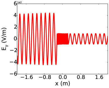
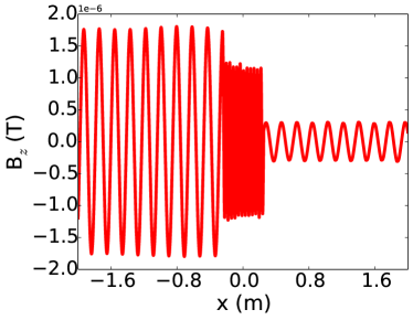
Figure 8: The 8y component of electric field and the 8 z component of the magnetic field of the EM wave of frequency 1.6 GHz traveling in a domain with plasma slab of thickness 0.3 m. The slab starts from x = -0.15 m. A background magnetic field of B_0x = 1 T is applied in the domain.

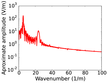
Figure 9: The wave number of the plane wave in neutral fluid and plasma.

IV Electromagnetic wave propagation over the RAM C

IV.1 Blackout

For the current problem, in the Eqs.(18)–(20), the advection and viscous diffusion occur on much larger time scales when compared to the time scale of the plasma oscillations and EM wave. For instance, the smallest advection and diffusion time scales in the stagnation region are $4.8\times 10^{-6}$ and $8.9\times 10^{-6}$ s respectively. Whereas the plasma oscillations occur on the time scale of $1.1\times 10^{-11}$ s. In the aft region (y=-1.25m), the minimum advection and diffusion times are $2.73\times 10^{-7}$ and $1.78\times 10^{-6}$ s respectively. The plasma frequency time scale is $1.01\times 10^{-10}$ s. Overall, the timescales of the advection and diffusion are more than three orders of magnitude the plasma oscillation time scale. Hence, the advection and the viscous diffusion terms are neglected. Note that the length scale used in the estimation of time scales is the average edge length of the local cell. The collision term in Eqs.(18)–(20) is neglected too as the collision frequencyrambo1994interpolation ; rambo1995comparison of the electrons and neutrals is less than an order of magnitude the plasma frequency. Figure 10 shows the comparison. The contour flood in Fig.10represents the plasma electron frequency and the contour lines show the electron neutral collision frequency. In the present simulation, the electron neutral collision frequency is highest among the collisions of the remaining species. The highest values of the frequencies are seen near the stagnation region, where the densities are high. The contours clearly show that plasma frequency is higher than the collision frequency everywhere within the plasma layer. Also, a line plot comparison along the stagnation line is shown in Fig.10 to get a better picture of the comparison of magnitudes.

The Eqs. (18)–(20) (advection, diffusion and collision terms neglected) are solved for ion and electron transport. The boundary conditions for the ions and electrons are same as that of the bulk fluid mentioned in Sec. III.1. The electron and ion densities are initialized using the reactive flow solution. For the Maxwell’s equations, conductor boundary condition is applied on the wall, which makes $\vec{n}\times\vec{E}$ and $\vec{n}\cdot\vec{B}$ zero.munz2000afinitevolume On all other boundaries, gradient of electric and magnetic fields is zero.

The wave reflection by the plasma layer of the RAM C is shown in Fig.11. The frequency of the plane wave originating at the top boundary is 1.6 GHz. The wave components at the top boundary are E_x = $ca_{0}sin(2\pi ft)$, B_z = E_y/c and the remaining components are equal to zero. Figures 11 and 11 represent the x,y components of the electric field. Figure 11 represents the z-component of the magnetic field. The contour flood shows the amplitudes of the wave. The dashed contour lines represent the plasma frequency. The inner most contour line seen near the nosecap corresponds to 16 GHz. The middle and outer most contour lines correspond to 1.6 Ghz and 0.16 GHz respectively. It can be clearly observed from the figures that the wave is completely reflected by the plasma layer once the plasma frequency is 1.6 GHz. Note that the flood contour levels are limited between peak positive and negative amplitudes of the original wave, in order to make the wave visible. The wave’s amplitude increases by about 10 times at the edge of the plasma layer due to the resonance of the evanescent wave.white1974amplification The amplified wave propagates along the plasma layer’s edge.

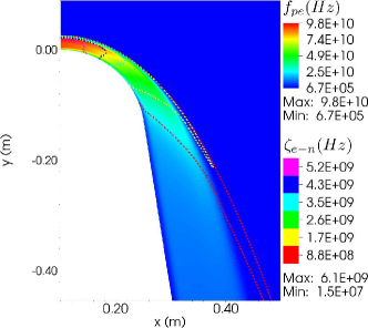
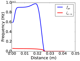
Figure 10: Comparison of the plasma electron frequency $f_{pe}$ and the collision frequency of electrons with neutrals $\zeta_{e-n}$. 10 contour lines of $\zeta_{e-n}$ and the contour flood of $f_{pe}$ and the 10 line plot of the frequencies along the stagnation line.

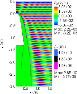
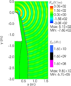
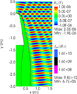
Figure 11: EM wave reflection in the plasma layer of RAM C. 11 x component of the electric field, 11 y component of the electric field, and 11 z component of the magnetic field. E_z, B_x, and B_y are zero. The contour lines represent the plasma electron frequency.

IV.2 Magnetic window whistler mode

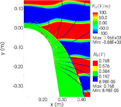
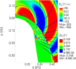
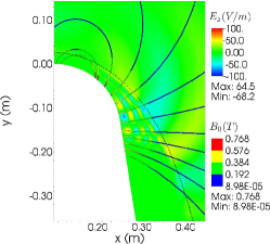
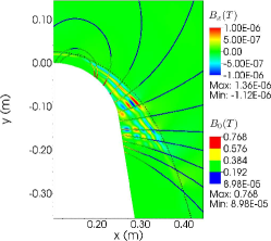
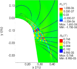
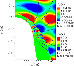
Figure 12: EM wave propagation in whistler mode in to the plasma layer of RAM C. The imposed magnetic field is shown by the streamlines. The three components of the electric and magnetic field are shown by the contour floods of 12, 12, 12, 12, 12, 12 respectively. The black dashed contour line corresponds to the electron plasma frequency of 1.6 GHz.

The magnetic field is applied on the surface near to the nosecap using a current carrying coil of radius 0.1 m centered at (0.15, -0.15). The coil’s axis is normal to y-axis and lies in the xy plane. The current is $1.5\times 10^{5}$ A. In practice a permanent magnet would be used to generate the field. The magnetic field lines colored in magnitude can be seen in all of the subplots of Fig.12. The maximum field strength available on the RAM C surface is 0.77 T while the value is around 0.125T at the the edge of the plasma layer where significant propagation of wave occurs. These magnetic field strengths are slightly large, however, many hypersonic vehicles of interest will actually have a considerably smaller plasma density and thus require a much weaker field to allow whistler wave propagation - this situation described can be considered an extreme case. In addition, it’s possible that using a weaker field will still allow whistler wave propagation as the evanescent waves may propagate through the outer edge of the plasma where the field is weak, then propagate as whistler waves closer to the vehicle surface. Figure 12 shows the flood contours of electric and magnetic field components of the EM wave. The cutoff frequency of plasma $f_{pe}$ = 1.6 GHz is depicted by the dashed contour line. The three components of the electric and magnetic field are shown in Figs.12-12 and Figs.12-12 respectively. It has to be noted that, the electric field contours are limited between -100 and 100 V/m, in order to improve the visibility of the whistler wave. It is clear now that the wave signal propagates through the plasma layer in the whistler mode. The additional components E_z, B_x, and B_y arising in Fig.12 when compared to the Fig.11 are due to the circular polarization of the wave around the magnetic field lines. The circularly polarized wave propagates parallel to the magnetic field lines. Hence the angle between the wave vector and the magnetic field lines at the edge of the plasma layer plays an important role. The wave does not propagate along the field lines perpendicular to the direction of propagation. It can also be observed from the figure that the magnetic window not only allows the passage of the original electromagnetic wave, it also focuses the wave through the converging magnetic field, which is in agreement with the observations made in Ref.takechi1999rf .

The ability to recover the original signal on the surface can be checked to verify that a useable signal can be obtained. The best way to do this is to find the frequency of the signal and its energy density at the surface. The frequency of the whistler wave is obtained by taking Fourier transform of the wave history recorded on the surface of RAM C. Figure 13 shows the frequency of E_x at (0.25555, -0.15829). The highest peak corresponds to a frequency of 1.6 GHz verifying that the original signal can be recovered at the vehicle surface.

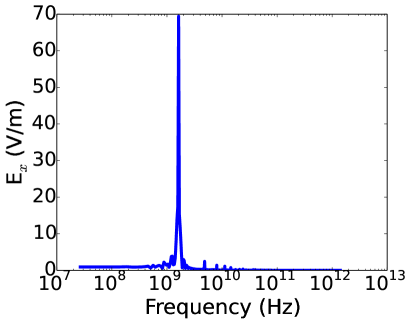
Figure 13: Whistler wave frequency on the surface of RAM C.

$$Q_{EM}=\frac{1}{2}\left(\epsilon_{0}\vec{E}\cdot\vec{E}+\frac{1}{\mu_{0}}\vec{B}\cdot\vec{B}\right)$$ (32)

In addition to the frequency match, the signal strength can also be calculated. The comparison of the energy density of the signal in the free space and that on the surface gives an idea of the signal strength. The wave’s energy density is computed using Eq. (32). A comparison of the electromagnetic energy density of the wave in the free space and that of the whistler wave on the surface of RAM C at (0.25555, -0.15829) is shown in Fig. 14. The Fig.14 corresponds to the wave in the free space and the bottom subplot is for the whistler wave. The slight rise in the energy of the free space wave at t = 4.5 ns is due to the added reflected components. It can be seen from Fig.14 that the whistler wave’s energy is sufficient to be received by the antenna. The whistler wave’s energy density is about 40$\%$ that of the original wave.

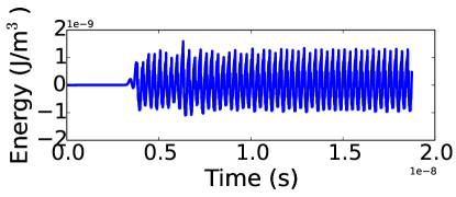
Figure 14: The energy density recorded in the free space and on the surface of RAM C. The maximum magnetic field on the RAM C surface is 0.77 T and the magnetic field at the plasma layer’s edge where the wave propagates is 0.125 T. 14 Recorded in free space and 14 on the RAM C surface at (0.25555, -0.15829).

Another interesting observation made during the simulations is the amplification of the whistler wave energy density with the increase of magnetic field. For instance, increasing the coil current by 4 times generates a maximum magnetic field of 3.1 T on the surface. The strength of the magnetic field at the plasma layer’s edge where the whistler wave propagation occurs in this case is around 0.8 T. The wave energy density history in a magnetic widow created with the increased magnetic field is shown in Fig.15. The energy density in this case is 400$\%$ of the source wave. In fact, the energy is amplified by about four times the wave’s energy in the free space. As explained previously, the amplification is due to the focusing of wave along the converging field lines. This amplification could be useful in the cases where, the original signal itself is weak.

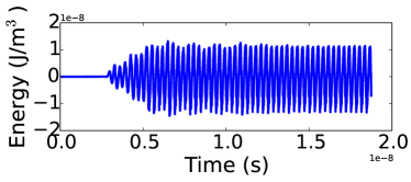
Figure 15: The recorded energy density on the surface of RAM C at (0.258043, -0.172272). The maximum magnetic field on the RAM C surface is 3.1 T and the magnetic field at the plasma layer’s edge where the wave propagates is 0.8 T.

From the above feasibility analysis, it can be said that the magnetic window subjected to a realistic flight condition is capable of propagating the signal on to the vehicle’s surface with energy densities ranging from 40$\%$ to 400$\%$ using magnetic fields of 0.15T and 0.8 T respectively at the edge of the plasma layer. However, the configuration can be further optimized by changing the orientation of the magnetic field lines after obtaining the plasma distributions for all the critical flight conditions in terms of angle of attack, speed and altitude.

The designer can also test other mitigation methods using the same model described in this paper. For instance, the electrophilic fluid injection method can be tested by adding the additional reactions to the existing reactions set of the multi-species transport equations to establish the reduced plasma density. The electron acoustic wave transmission can be tested by including the multi-fluid advection terms in the analysismudaliar2012radiation so that the electron acoustic wave is simulated. Similarly, resonant transmission can be modeled with the equations described.

V Conclusions

A procedure to model and simulate the hypersonic flow and the vehicle’s communication blackout is shown. The plasma density on the RAM C vehicle showed good agreement with the reflectometer measurements from the literature. Addition of radiation losses to the reactive flow could further improve the accuracy the simulation results. The results of the Maxwell equation solver of USim are validated with the analytical solution of whistler wave propagation in one dimensional plasma layer. The Whistler mode propagation of the wave on the RAM C surface is demonstrated successfully. The frequency and the energy density of the wave signal recorded on the surface of RAM C showed a good possibility of recovering the signal propagated in whistler mode. Although only the magnetic window is investigated, the same plasma model together with the solver can be used to investigate many radio blackout mitigation schemes including electron acoustic wave transmission and resonant transmission.

References

References

- (1) Bertin, J. J.,“Hypersonic aerothermodynamics,” AIAA Education Series, AIAA, 1994, pp.4–5.
- (2) Hodara, H, "The use of magnetic fields in the elimination of the re-entry radio blackout", Proceedings of the IRE, Vol. 49, No. 12, 1961.
- (3) Manning, R. M., “Analysis of electromagnetic wave propagation in a magnetized re-entry plasma sheath via the Kinetic equation,” NASA/TM–2009-216096, 2009.
- (4) Thoma, C., Rose, D.V., Miller, C.L., Clark, R.E. and Hughes, T.P., “Electromagnetic wave propagation through an overdense magnetized collisional plasma layer,” Journal of Applied Physics, Vol. 106, No.4, 2009, pp. 043301.
- (5) Starkey, R. P., “Electromagnetic Wave/Magnetoactive Plasma Sheath Interaction For Hypersonic Vehicle Telemetry Blackout Analysis," 34th AIAA Plasmadynamics and Lasers Conference, Orlando, Florida, June 2003.
- (6) Usui, H., Matsumoto, H., Yamashita, F., Yamane, M., and Takenaka, S., “Computer experiments on radio blackout of a reentry vehicle," 6th Spacecraft Charging Technology, Vol. 1, 2000, pp. 107–110.
- (7) Meyer, J.W., Lockheed Martin Corp., Palo Alto, CA, U.S. Patent “System and method for reducing plasma induced communication disruption utilizing electrophilic injection and sharp reentry vehicle nose shaping,” Publication No. US7237752 B1, filed 18 May. 2004.
- (8) Gillman, E. D., Foster, J. E. and Blankson, I. M., “Review of leading approaches for mitigating hypersonic vehicle communications blackout and a method of ceramic particulate injection via cathode spot arcs for blackout mitigation”, NASA TM–2010-216220, 2010.
- (9) Keidar, M., Kim, M. and Boyd, I., “Electromagnetic reduction of plasma density during atmospheric reentry and hypersonic flights",Journal of Spacecraft and Rockets, Vol. 45, No. 3, 2008, pp. 445–453.
- (10) Sternberg, Natalia and Smolyakov, Andrei I, “Resonant transmission of electromagnetic waves in multilayer dense-plasma structures,” IEEE Transactions on Plasma Science, Vol. 37, No. 7, 2009.
- (11) Stenzel, R. L. and Urrutia, J. M., “A new method for removing the blackout problem on reentry vehicles,” Journal of Applied Physics, Vol. 113, No. 10, 2013, 103303.
- (12) Mudaliar, Saba and Sotnikov, Vladimir I, "Radiation Characteristics of Antennas Embedded in a Medium With a Two-Temperature Electron Population", Antennas and Propagation, IEEE Transactions on, Vol. 60, No. 10, 2012. DOI:10.1109/TAP.2012.2207314.
- (13) Stenzel, R. L., “Whistler wave propagation in a large magnetoplasma,” Physics of Fluids, Vol. 19, No. 6, 1976, pp.857–864.
- (14) Takahashi, Yusuke and Yamada, Kazuhiko and Abe, Takashi,“Prediction Performance of Blackout and Plasma Attenuation in Atmospheric Reentry Demonstrator Mission,”Journal of Spacecraft and Rockets. DOI: 10.2514/1.A32880.
- (15) Takahashi,Y., Yamada, K. and Abe, T., “Examination of Radio Frequency Blackout for an Inflatable Vehicle During Atmospheric Reentry,” Journal of Spacecraft and Rockets, Vol. 51, No. 2, 2014, pp. 430–441.
- (16) Visbal, Miguel R and Sherer, Scott E and White, Michael D, "High-Order Methods For Wave Propagation", Air Force Research Lab, ADA476109, Wright-Patterson AFB, OH, Jan 2008.
- (17) Jones, W.L.Jr. and Cross,A.E., “Electrostatic-probe measurements of plasma parameters for two reentry flight experiments at 25000 feet per second,”NASA TN D-6617, Washington, D.C., Feb 1972.
- (18) Shashurin, A., Zhuang, T., Teel, G., Keidar, M., Kundrapu, M., Loverich, J., Beilis, I.I. and Raitses, Y., “Laboratory Modeling of the Plasma Layer at Hypersonic Flight,” Journal of Spacecraft and Rockets, Vol. 51, No. 3, 2014, pp. 838–846.
- (19) Loverich, J., Zhou, S. CD., Beckwith, K., Kundrapu, M., and Loh, M., Mahalingam, S., Stoltz, P. and Hakim, A., “Nautilus: A Tool for Modeling Fluid Plasmas,” 51st AIAA Aerospace Sciences Meeting including the New Horizons Forum and Aerospace Exposition, Grapevine, TX, Jan 2013.
- (20) Kundrapu, M., Loverich, J., Beckwith, K., Stoltz, P., Keidar, M., Zhuang, T. and Shashurin, A., “Modeling and Simulation of Weakly Ionized Plasmas Using Nautilus,” 51st AIAA Aerospace Sciences Meeting including the New Horizons Forum and Aerospace Exposition, Grapevine, TX, Jan 2013.
- (21) Munz, C-D., Ommes, P., and Schneider, R., “A three-dimensional finite-volume solver for the Maxwell equations with divergence cleaning on unstructured meshes," Computer Physics Communications, Vol. 130, No. 1, 2000, pp. 83–117. DOI: 10.1016/S0010-4655(00)00045-X
- (22) Zhdanov, V. M., “Transport Processes in Multicomponent Plasma,” Taylor and Francis, Philadelphia, 2002, pp. 53–58.
- (23) Kumar, Harish and Mishra, Siddhartha, “Entropy stable numerical schemes for two-fluid plasma equations", Journal of Scientific Computing, Vol. 52, No. 2, 2012.
- (24) Loverich, John and Hakim, Ammar and Shumlak, Uri, “A discontinuous Galerkin method for ideal two-fluid plasma equations", Communications in Computational Physics, Vol. 9, No. 2, 2011.
- (25) Shumlak, U. and Loverich, J.,“Approximate Riemann solver for the two-fluid plasma model”, Journal of Computational Physics, Vol. 187, No. 2, 2003, pp.620–638.
- (26) Shumlak, U and Lilly, R and Miller, S and Reddell, N and Sousa, E, “High-order finite element method for plasma modeling",Pulsed Power Conference, San Francisco, CA, June 2013, pp. 1–5. DOI:10.1109/PPC.2013.6627593.
- (27) Srinivasan, Bhuvana and Hakim, Ammar and Shumlak, Uri, “Numerical methods for two-fluid dispersive fast MHD phenomena",Communications in Computational Physics, Vol. 10, 2011.
- (28) Hakim, A., Loverich, J. and Shumlak, U., “A high resolution wave propagation scheme for ideal Two-Fluid plasma equations,” Journal of Computational Physics, Vol. 219, No. 1, 2006, pp.418–442.
- (29) Thompson, Richard Joel., “Fully coupled fluid and electrodynamic modeling of plasmas: a two-fluid isomorphism and a strong conservative flux-coupled finite volume framework,” Dissertation, University of Tennessee Space Institute, 2013.
- (30) Johnson, Evan Alexander., "Gaussian-Moment Relaxation Closures for Verifiable Numerical Simulation of Fast Magnetic Reconnection in Plasma",Disseration, University Of Wisconsin–Madison, 2013.
- (31) Leer, V.B., “Towards the ultimate conservative difference scheme. V. A second-order sequel to Godunov’s method,” Journal of computational physics, Vol. 32, No. 1, 1979, pp. 101–136.
- (32) Einfeldt, B., “On Godunov-type methods for gas dynamics,” SIAM Journal on Numerical Analysis, Vol. 25, No. 2, 1988, pp. 294–318.
- (33) Ahnert, K. and Mario M., “Odeint-Solving ordinary differential equations in C++,” arXiv preprint arXiv:1110.3397, 2011.
- (34) Josyula, E. and Bailey, W.F.,“Governing equations for weakly ionized plasma flowfields of aerospace vehicles,” Journal of spacecraft and rockets, Vol. 40, No. 6, 2003, pp. 845–857.
- (35) Blacker, T. D., William, J. B. and Tony L. E., “CUBIT mesh generation environment. Volume 1: Users manual. No. SAND–94-1100,” Sandia National Labs, Albuquerque, NM (United States), 1994.
- (36) Grantham, W. L., “Flight results of a 25000-foot-per-second reentry experiment using microwave reflectometers to measure plasma electron density and standoff distance,” NASA-TN-D-6062, L-7107, Dec 1970.
- (37) Goldston, R. J. and Rutherford, P.H., “ Introduction to plasma physics,”CRC Press, 2000, pp.277–284.
- (38) Jenkins, T. G., Austin, T. M., Smithe, D. N., Loverich, J. and and Hakim, A. H.,“Time-domain simulation of nonlinear radiofrequency phenomena”, Physics of Plasmas, Vol. 20, No. 1, 2013, 012116.
- (39) Merritt, E. C., Moser, A. L., Hsu, S. C., Loverich, J. and Gilmore, M.,“Experimental characterization of the stagnation layer between two obliquely merging supersonic plasma jets”, Physical Review Letters, 111, Aug 2013, pp. 085003. DOI:10.1103/PhysRevLett.111.085003.
- (40) Rambo, P. W. and Denavit, J. “Interpenetration and ion separation in colliding plasmas,” Physics of Plasmas (1994-present), Vol. 1, No. 12, 1994, pp. 4050–4060.
- (41) Rambo, P. W. and Procassini, R. J., “A comparison of kinetic and multifluid simulations of laser-produced colliding plasmas,” Physics of Plasmas (1994-present), Vol. 2, No. 8, 1995, pp.3130–3145.
- (42) Munz, C. D., Schneider, R. and Voss, U., “A finite-volume method for the Maxwell equations in the time domain,” SIAM Journal on Scientific Computing, Vol. 22, No. 2, 2000, pp.449–475. DOI:10.1137/S1064827596307890.
- (43) White, R. B. and Chen, F. F.,“Amplification and absorption of electromagnetic waves in overdense plasmas”, Plasma Physics, Vol. 16, 1974, pp.565–587.
- (44) Takechi, S. and Shunjiro, S., “Rf wave propagation in bounded plasma under divergent and convergent magnetic field configurations,” Japanese journal of applied physics, Vol. 38, No. 11A, 1999,pp. 1278–1280.