Photoelectric effect induced by blackbody radiation: a theoretical analysis of a potential heat energy harvesting mechanism

Abstract

The photoelectric effect induced by blackbody radiation could be a mechanism to harvest ambient thermal energy at a uniform temperature. Here, I describe (without going too much into mathematical details) the theoretical model I developed starting from 2010 to study that phenomenon, and I summarize the results of the numerical simulations. Simulations tell us that the process must be there. Moreover, at least two experimental tests have been performed in the past years that seem to corroborate, although not definitely, the alleged functioning of the proposed mechanism. Unfortunately, at present, the obtainable power density is extremely low and inadequate for immediate practical applications.

Keywords: second law of thermodynamics $\cdot$ blackbody radiation $\cdot$ photoelectric effect $\cdot$ thermionic emission $\cdot$ work function $\cdot$ Kirchhoff’s loop rule

1 Introduction

If we can get energy from ambient light via the photoelectric effect, why should it not be possible to harvest ambient thermal energy at a uniform temperature through the photoelectric effect caused by blackbody radiation? In the paper, I sometimes refer to this second process as the thermionic emission. What I will present here is a theoretical analysis of that possibility, and it stands on my work on that topic dating back to 2010 [1, 2, 3, 4, 5, 6, 7, 8, 9]. I anticipate that the answer is affirmative in principle. Unfortunately, the obtainable power density turns out to be extremely low and inadequate for immediate practical applications. Due to its simplicity, this idea is not new. It has already been proposed and even experimentally approached (Section 5), but usually with what appears to be a not fully satisfying theoretical explanation. Here, I describe my contribution to remedying this lack, also because, as Sir. Eddington put it, you should not put much confidence in experimental results until they have been confirmed by theory.

2 The basic idea

The idea behind the approach proposed in this paper is simple: exploiting the photoelectric effect of the ambient blackbody radiation (at a uniform temperature) on materials with different work functions $\phi$. The simplest design to do that is shown in Fig. 1.

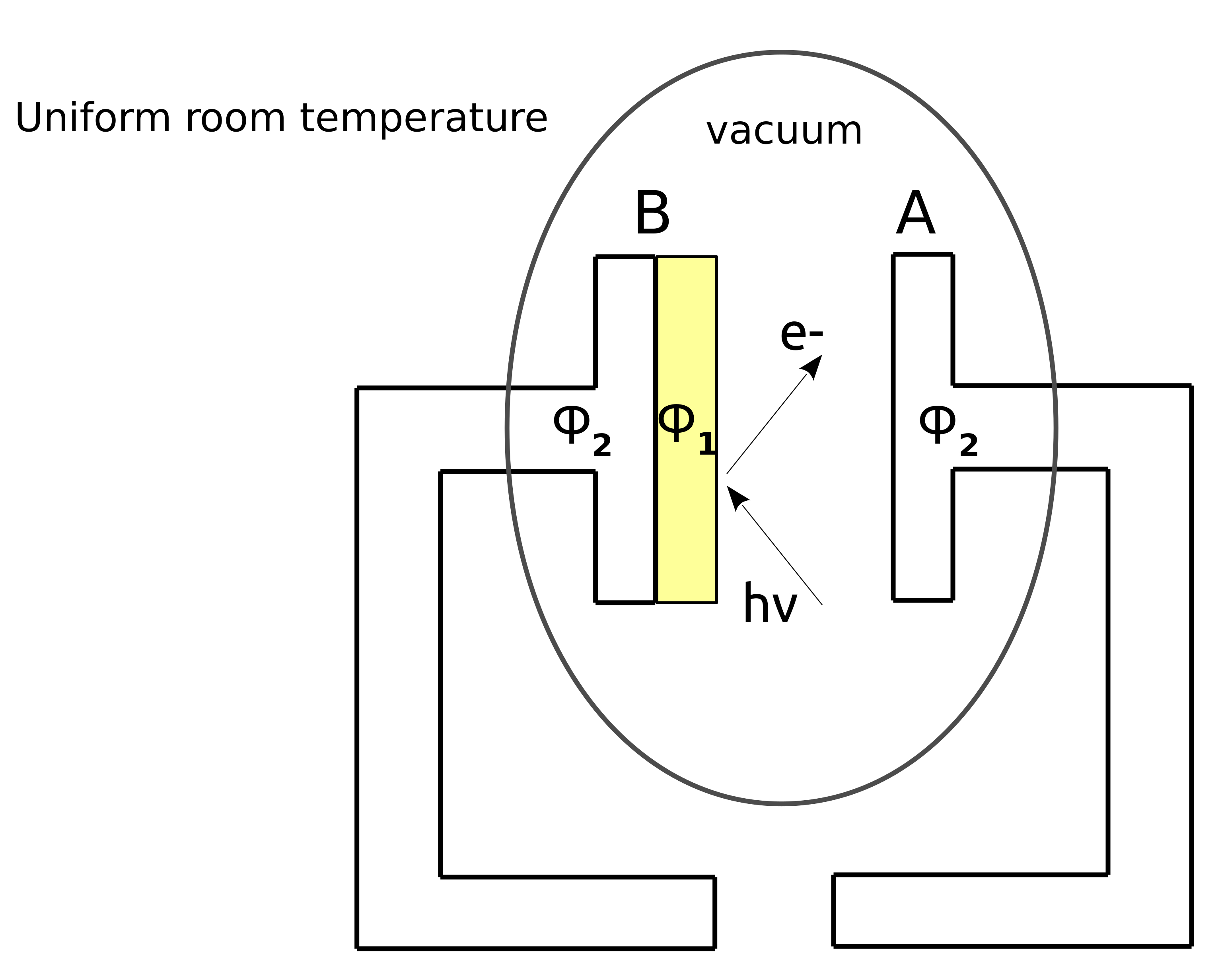
Figure 1: Sketch of a thermo-charged capacitor (TCC)

The sketched device is a capacitor, which I dubbed “thermo-charged capacitor” (or TCC), where two plates, A and B, are housed inside a vacuum bulb. Plate A and part of plate B are made of the same metal with work function $\phi_{2}$. Plate B is coated with a semiconductor with a lower work function $\phi_{1}$. The whole device is at a uniform temperature.

Both plates A and B receive photons from the blackbody radiation, but being $\phi_{2}$ greater than $\phi_{1}$, the electrons extracted by the photoelectric effect from the coating of B to plate A are more numerous and with higher kinetic energy $K$ ($K=h\nu-\phi$, where $h\nu$ is the photon energy) than those extracted from plate A to plate B, at least in the early phases of the process.

This behavior is evident when we look at the shape of the spectral radiance vs. the frequency of the blackbody radiation at equilibrium (uniform temperature), Fig. 2.

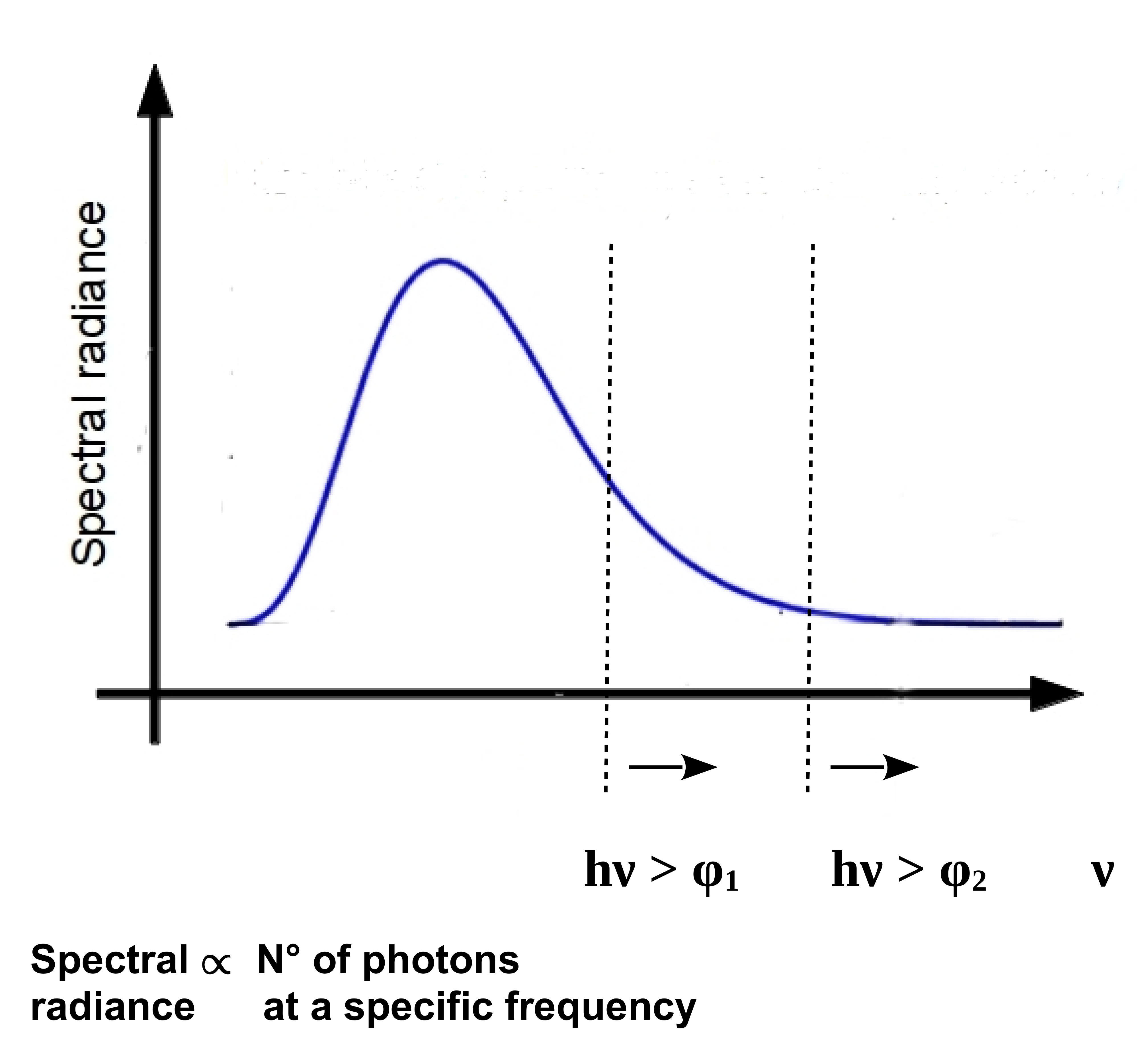
Figure 2: Blackbody radiation at a uniform temperature. The spectral radiance is proportional to the number of blackbody photons at a specific frequency

The spectral radiance being proportional to the number of blackbody photons at a specific frequency, the number of photons in the thermal radiation with energy $h\nu>\phi_{1}$ is greater than the number of photons with $h\nu>\phi_{2}$, and thus it is easy to see why more electrons are extracted from B to A and with higher kinetic energy. All that means that an unbalanced net flux of electrons should flow from plate B to plate A.

To show how the TCC is expected to work, it may help to consider the following two distinct setups: open-circuit and short-circuit TCC, see Fig. 3. In the case of an open-circuit TCC (Fig. 3, left), we expect that after a suitable interval of time, an equilibrium potential difference $\Delta V$ gets established across the plates.

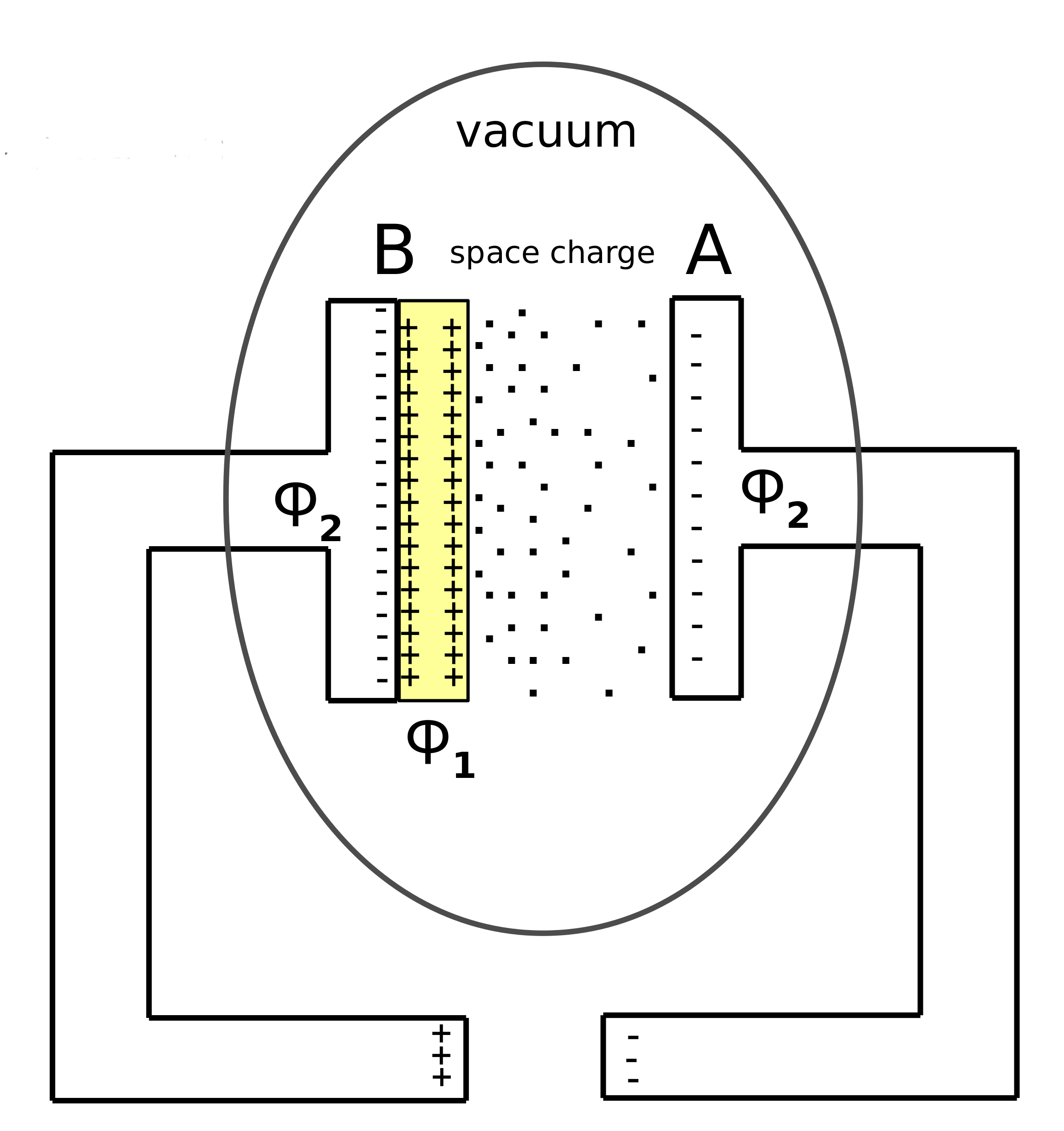
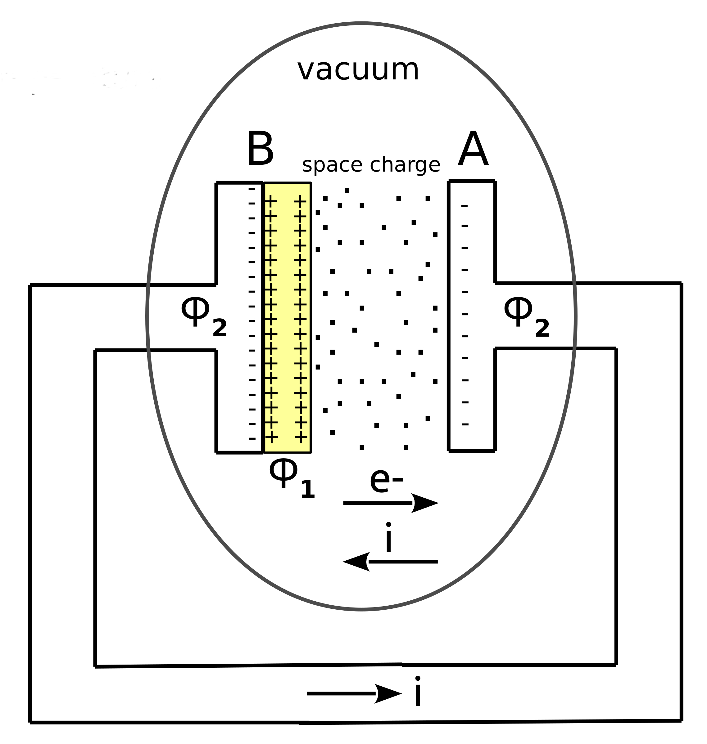
Figure 3: Open-circuit (left) and short-circuit (right) TCCs

The equilibrium potential difference $\Delta V$ is necessarily equal to $(\phi_{2}-\phi_{1})/e$, where $e$ is the electron charge, because only with that value the energy $E_{B}$ needed by an electron inside the coating to get extracted and reach plate A ($E_{B}=\phi_{1}+e\Delta V=\phi_{1}+e(\phi_{2}-\phi_{1})/e=\phi_{2}$) becomes equal to the energy $E_{A}$ needed by an electron to get extracted from plate A and reach plate B (only $\phi_{2}$). Only in this case, there will be no more imbalance in the two fluxes of electrons.

In the case of a short-circuit TCC (Fig. 3, right), a current $i$ should flow in the circuit. If the resistance of the circuit external to the TCC is negligible, that current is equal to the thermionic current $i_{thermionic}$ across the plates, and the potential difference between the plates is nearly equal to zero.

The small dots between the plates represented in Fig. 3, especially in the open-circuit TCC configuration, is the space charge. In stationary conditions like that of a fully charged open-circuit TCC, electrons are continuously emitted and reabsorbed by the plates in a sort of dynamical equilibrium, and thus they form a cloud. This is well-known among those who used to work with vacuum tubes. Space charge distribution inside a TCC can be modeled mathematically, but it is not difficult to understand that in an open-circuit configuration at equilibrium, the electron cloud density decreases from plate B to plate A (fewer and fewer electrons in plate B get enough energy from the blackbody radiation to get closer and closer to plate A).

Notice that this space charge does not change the value of the total stationary potential drop between the plates, which always remains equal to $(\phi_{2}-\phi_{1})/e$ for the reasons explained above. The space charge interferes only with the uniformity of that potential in the inter-plate space: the potential difference does not change linearly with the distance from the plates as it happens in a standard charged parallel-plate capacitor.

3 Possible objections to the expected functioning

Before presenting the results of the mathematical and numerical modeling of both open-circuit and short-circuit TCCs, let me dwell on two main objections that could be advanced against the functioning described above. It is fundamental to face the following objections and reply to them because, if they were correct, the TCC would not work as expected.

To better introduce them, I will use a topological analog of the short-circuit TCC in Fig. 3 (right). I refer to the horseshoe-shaped scheme shown on the right-hand side of Fig. 4. The right half of the horseshoe represents plate A, part of plate B, and the connecting wire, and all this stuff has a work function equal to $\phi_{2}$. The left half is the coating of plate B with work function $\phi_{1}$. In both images, J-II indicates the vacuum gap between the plates.

It is known that when two materials with different work functions are physically joined, a potential difference $\Delta V_{bi}$ builds up across the contact junction J-I (Fig. 4, right). This potential is known as the contact potential, and it is generated by electrons that are pushed from the $\phi_{1}$ material to the $\phi_{2}$ material across J-I by thermally driven forces (thermal agitation).

Figure 4: Short-circuit TCC (left) and its topological analog (right)

A higher amount of electrons move from left to right rather than the other way around simply because it’s easier to pull electrons out of a lower work function material. This process lasts until a dynamical equilibrium is reached between the thermally driven forces and the electric force due to the built-in electric field across J-I.

Also, in this case, the contact potential $\Delta V_{bi}$ across J-I is equal to $(\phi_{2}-\phi_{1})/e$, and the reason is the same as that shown in Section 2 for the final equilibrium of the thermionic charging process. Across J-I, an electric field builds up as well. It is roughly equal to the contact potential divided by the width of the depletion region $x_{d}$, namely the thin layer across J-I where the diffusion of electrons has taken place.

It is also widely held that as soon as the two halves of the horseshoe are physically joined at J-I, a potential difference, equal and opposite to the contact potential $\Delta V_{bi}$ at J-I, should instantaneously build up across the gap J-II.

That potential difference must not be confused with that deriving from the thermionic charging process described in Section 2. It is intended to be instantaneously generated by the movement of electrons in the bulk of the horseshoe just after the physical contact of the materials at J-I. People expect that potential difference across J-II because of an allegedly straightforward application of Kirchhoff’s loop rule to the horseshoe scheme in Fig. 4.

The first objection to the TCC functioning is that if this potential difference really formed across J-II, the thermionic charging process across plates A and B would not even start. Since $\Delta V$ across J-II is equal to $(\phi_{2}-\phi_{1})/e$, no net electron flux from plate B to plate A could be possible. As described in Section 2, the energy required for an electron to get extracted from one plate and reach the other plate would be the same (and incidentally, equal to $\phi_{2}$). Thus, there would be no net displacement of electrons across J-II, and therefore there would be no current in the short-circuit TCC.

My reply to that objection is that there is no instantaneous potential difference across J-II caused by physically joining the two materials at J-I. And I can prove it by appealing to the basic definition of potential difference: the potential difference between points $a$ and $b$ is defined as minus the work $W$ done by the forces acting upon a test electron that moves along a(ll) path(s) joining $a$ and $b$, divided by the electron charge $e$ [4, 6, 7, 8].

Figure 5: Definition of potential difference between points $a$ and $b$ in the bulk of the horseshoe

Let us apply that definition to the previous horseshoe scheme, see Fig. 5. Namely, $\Delta V_{ba}=V_{b}-V_{a}=-W_{ab}/e=-1/e\int_{a}^{b}{\bf F_{int}}\cdot d\boldsymbol{\gamma}$, where ${\bf F_{int}}$ stands for all the forces acting upon the test electron when it moves along the path $\gamma$.

If one considers the path $\gamma$ shown in Fig. 5, it is evident from equilibrium considerations that ${\bf F_{int}}$ can be different from zero only across J-I. When the test electron crosses J-I, it does feel only two forces: the thermally driven forces ${\bf F_{d}}$ pushing to the right and the electric force $e{\bf E_{bi}}$ due to the built-in electric field pushing to the left, and thus ${\bf F_{int}}={\bf F_{d}}+e{\bf E_{bi}}$. By the way, the test electron does feel the thermally driven forces, just like all electrons in the depletion region around J-I.

Since the diffusion forces dynamically sustain the electric field at J-I, these two force fields must always be present across J-I and must always be equal and opposite at equilibrium, namely ${\bf F_{d}}=-e{\bf E_{bi}}$. As a matter of fact, if we switched off the thermally driven forces ${\bf F_{d}}$, the built-in electric field ${\bf E_{bi}}$ would go to zero. Therefore, the total force ${\bf F_{int}}$ is zero on average, and so is the potential difference $\Delta V_{ba}$ between points $a$ and $b$.

All that means that physically joining two different materials at J-I cannot instantaneously cause any potential drop across the gap J-II that would kill the thermionic emission from the outset.

That theoretical result may appear at odds with the fact that a potential difference $\Delta V$ is actually detected and measured across J-II among different materials physically joined at J-I. For instance, measuring this $\Delta V$ is one of the reasons why the Kelvin probe force microscope (KPFM) has been developed. My explanation for this apparent inconsistency is that KPFM, in fact, measures a potential difference across J-II, but this potential difference is just that generated by thermionic emission across J-II. In the case of a KPFM scan, I am referring to the thermionic emission between the surface of the scanned material and the Kelvin probe tip. The potential difference measured by a KPFM is thus not that due to the contact potential at J-I.

The second objection to the expected functioning of a TCC is that even if a net flux of emitted electrons were possible from left to right across J-II (see, Fig. 5), the current would not flow back across junction J-I. Junction J-I is known to be a Schottky-type rectifying junction: under biasing, electrons easily flow from left to right across J-I but not that easily the other way around (from right to left across J-I).

The reply to that objection is simple and more immediate [2, 8]. It is well known that every Schottky junction is characterized by a reverse leakage current that overcomes the rectifying barrier even under small reverse biasing. That current may be high or low depending upon several factors. It depends (although slightly) upon the magnitude of the reverse bias. It also depends upon junction materials and preparation. It is proportional to the temperature and has an inverse dependence upon the depletion region width $x_{d}$. According to the literature, the reverse leakage current may range from $10^{-8}$ A/cm² to $10^{-2}$ A/cm² (there also exist examples of higher values), and as I will show in the next section, even the lowest value is already enough to allow the circulation of a current through a short-circuit TCC (Fig. 3, right).

4 Numerical simulation and results

I have mathematically modeled the photoelectric effect induced by the electromagnetic radiation following Plank’s law (blackbody radiation) on both plates of a spherical capacitor (with different work functions). Here, I describe the results of the numerical simulation. I have studied a spherical TCC (see Fig. 6) because it is easier to treat analytically [2, 8].

Figure 6: Sketch of the modeled open-circuit spherical TCC

For the low work function coating, I have chosen the well-known photo-cathode material S1 (Ag-O-Cs) with a work function of nearly 0.7 eV. The inner and outer spheres are made of metal with a work function of 4 eV. The modeled TCC is 40 cm wide ($b=20$ cm and $a=10$ cm). The ratio between the outer and the inner radius is taken equal to 2 because it can be proven that this choice maximizes the charging speed in the open-circuit setup [1].

Another significant parameter for the simulation is the quantum efficiency $\eta$ of the materials. The quantum efficiency is roughly the ratio between the number of electrons extracted by the radiation and the number of photons impinging on the plates. It is a frequency-dependent parameter. I have plugged into the equations only mean values over frequency. I have used highly conservative values for the quantum efficiencies to stress-test the robustness of the process: $\eta_{1}=10^{-5}$ and $\eta_{2}=1$. More realistic values are $\eta_{1}\geq 10^{-3}$ ($\geq 0.1\%$) [11] and $\eta_{2}\ll 1$. Moreover, I have found the whole process and results to be quite insensitive to the exact value of $\eta_{2}$.

The differential equation that governs the charging process of an open-circuit spherical TCC is the following [2, 8]:

$$\frac{dV(t)}{dt}=\frac{\pi eb}{2\epsilon_{0}c^{2}}\biggl{(}\frac{kT}{h}\biggr{)}^{3}\Biggl{(}\overline{\eta}_{1}\int_{\frac{eV(t)+\phi_{1}}{kT}}^{\infty}\frac{x^{2}dx}{e^{x}-1}-4\overline{\eta}_{2}\int_{\frac{\phi_{2}}{kT}}^{\infty}\frac{x^{2}dx}{e^{x}-1}\Biggr{)},$$

where $V(t)$ is the voltage between the spheres, $b$ is the radius of the outer sphere, $c$ is the velocity of light, $e$ is the electron charge, $\epsilon_{0}$ is the vacuum permittivity, $h$ is the Planck constant, $T$ is the absolute temperature, and $k$ is the Boltzmann constant.

The graph in Fig. 7 shows the charging profile of a spherical open-circuit TCC with the abovementioned parameters.

Figure 7: Charging profile of the open-circuit spherical TCC described in the text. Charging profiles for three absolute temperatures (296 K, 298 K, and 300 K) are given

With more realistic values for $\eta_{1}$ and $\eta_{2}$, the charging process is expected to be sensibly faster (one or two orders of magnitude faster).

When the terminals of the spherical TCC are connected to a resistor $R$, a current starts to flow across the circuit and settles to a steady-state value $i_{S}$. That current is related to the steady-state voltage $V_{S}$ across $R$ and the TCC as follows [2, 8]:

$$i_{s}=\frac{2\pi^{2}eb^{2}}{c^{2}}\biggl{(}\frac{kT}{h}\biggr{)}^{3}\Biggl{(}\overline{\eta}_{1}\int_{\frac{eV_{s}+\phi_{1}}{kT}}^{\infty}\frac{x^{2}dx}{e^{x}-1}-4\overline{\eta}_{2}\int_{\frac{\phi_{2}}{kT}}^{\infty}\frac{x^{2}dx}{e^{x}-1}\Biggr{)},$$

and, obviously, they satisfy Ohm’s law $V_{S}=R\cdot i_{S}$.

The power density $P_{S}$ of the short-circuit spherical TCC is then given by $P_{S}=V_{S}\cdot i_{S}/S_{a}$, where $S_{a}$ is the surface of the inner sphere. The graph in Fig. 8 shows the power density $P_{S}$ as a function of the steady-state voltage $V_{S}$ in Watts/cm².

Figure 8: Power output per unit area of the inner sphere versus the steady-state voltage across the TCC and the resistor $R$ (for three values of the ambient temperature)

By tuning the value of the external resistance $R$, we can maximize the power output. The maximum is obtained at 0.03 V across a resistance of the order of $10^{10}~{}\Omega$. Therefore, the maximum power output reachable by the spherical TCC with the abovementioned physical characteristics is nearly $10^{-14}$ W, with a steady-state current of the order of $10^{-12}$ A.

By plugging into the equations more realistic values for $\eta_{1}$ and $\eta_{2}$, I expect to have a power output and a current at least two orders of magnitude higher, $P_{S}\approx 10^{-12}$ W and $i_{S}\approx 10^{-10}$ A.

The power output of the modeled TCC and the power density represented in Fig. 8 clearly show that the current design has no hope for an immediate application for large-scale ambient energy harvesting. However, it is crucial to experimentally prove it since only this way we will have confirmation that our approach is not at odds with fundamental physics.

5 About experimental tests

Before describing the two experiments I became aware of that seem to implement the design described above, let me linger over a few necessary (but not sufficient) prescriptions that every experimental test must comply with to be credible.

They are listed below in no particular order:

• Reduce external disturbance (varying electric and magnetic fields, e.m. pickup, cosmic rays, etc.) by properly shielding the TCC and the measurement equipment with Faraday cages and mu-metal boxes and by performing the test inside an underground laboratory;

• Carefully control the uniformity of the temperature to prevent thermoelectric effects: no significant temperature gradient should be allowed in the space hosting the TCC and the measurement equipment;

• Place two TCCs side by side: they must be the same, except that one does not have any emitting layer on its plates;

• Use an ultra-high input impedance electrometer ($>10^{10}\,\Omega$). According to the previous simulation, the resistance external to the TCC must be very high.

Another significant check to do would be using multiple equivalent TCCs. They should be connected in series or parallel to see whether the overall voltage and current scale up with the number of TCCs. If they do not, then any possible non-zero voltage and current values for a single TCC could easily be caused by noise in the measurement equipment. This check would be even more important than seeing whether the magnitudes of voltage and current on a single TCC correlate with ambient temperature: even the internal noise of a high-sensitivity electrometer correlates with ambient temperature.

At the end of 2014, I received, as personal communication, a report by Fu and Fu [10] on an experiment conducted on some Ag-O-Cs vacuum bulbs with custom design (see Fig. 9). They were previously employed by the same authors to test the possibility of drawing energy from ambient heat with the help of an external static magnetic field [9]. In that report, they actually implemented and tested the basic scheme of a thermo-charged capacitor like the one sketched in Fig. 1.

Figure 9: One of the vacuum tubes used by Fu and Fu [10]

How their original vacuum bulbs were manufactured (see Fig. 9) made Fu and Fu able to use the Ag-O-Cs plates A and B, connected in series, as the emitter and a cesium-coated molybdenum supporting rod facing the plates (P) as the collector of a simplified version of a thermo-charged capacitor. A schematic of the experiment, taken from Fu and Fu’s report, is given in Fig. 10, where the vacuum tube, a shielding copper box, and the measuring apparatus (electrometer Keithley 6514) are visible.

Figure 10: Schematic of the experiment carried out by Fu and Fu [10]

Fu and Fu measured a stable current exceeding $2\times 10^{-12}$ A and a voltage drop of the order of 100 mV. They also verified that both these values change sign once the electrometer’s connections to the tube are switched over. Unfortunately, they did not investigate the dependence of the current/voltage output on the number of connected tubes and the value of the external uniform temperature: the measurements described in the report have been taken on a single vacuum tube and at a single external temperature. Their results are extremely interesting and promising and seem to give a direct experimental corroboration of the theory behind the thermo-charging process. Their vacuum tube has probably an emitting surface of a few square centimeters. If we scale down the results presented in the previous Section by two orders of magnitude in the inner area and use the more realistic value for the quantum efficiency of the emitting surface ($\eta_{1}\geq 10^{-3}$), we see that the expected current for a single vacuum tube is of the same order of magnitude as that found by Fu and Fu.

In their report, Fu and Fu also ventured into a theoretical explanation for their results. However, in my opinion, they did not succeed. Unfortunately, their explanation is quite sketchy and presents some flaws at a fundamental level.

In May 2011, a person who read my first papers on the TCC sent me an email and drew my attention to the work of a Chinese researcher, Xu Yelin, which I was not aware of [12]. Yelin performed a large-scale experiment using nearly 700 custom Ag-O-Cs vacuum tubes connected in series (see Fig. 11). Although he did not use any ultra-high input electrometer, he found non-zero current and voltage across the circuit. In particular, at the ambient temperature of 32^∘ C, he measured a peak short-circuit output current of $\approx 5\times 10^{-8}$ A and a voltage drop of 55 mV across an external resistance of $10^{8}\,\Omega$. The interesting fact is that the current and voltage values remained stable for over a year (the duration of the experiment), with variations closely matching the ambient temperature trend.

Figure 11: Some of the schematics of the experiment carried out by Xu Yelin [12]

Even in this case, the emitting surface of a single vacuum tube is of the order of a few square centimeters, and thus the current generated by each tube is of the order of $10^{-12}$ A. Again, it seems to agree with the results of the simulations presented in the previous Section with $\eta_{1}\geq 10^{-3}$.

Yelin proposed a theoretical explanation for his results, but again it appears to be somewhat cursory and plagued by several flaws at a fundamental level. That notwithstanding, Yelin’s experiment and results remain fascinating.

To conclude this section, let me describe an indirect and easier way to test the expected functioning of a TCC [8]. Let us use the TCC as a conventional photoelectric device and exclusively illuminate the low work function plate (plate B in Fig. 1) with direct light of arbitrary intensity but with frequency $\nu<\phi_{2}/h$. The fact that plate A is not illuminated does not count since the light used has a too low frequency to extract electrons from it. In fact, that would be almost like having a TCC immersed in blackbody radiation with a higher intensity than usual and a frequency cutoff at $\phi_{2}/h$.

It should be easy to understand that if we can measure a non-zero potential difference and a non-zero current in the open-circuit and short-circuit configurations, respectively, then the TCC should work as expected even when it is immersed in uniform blackbody radiation as in the original design. The only difference would be in the rapidity with which the potential difference is generated or the magnitude of the current in the short-circuit configuration. Those would be more favorable in the case of the TCC used like a photoelectric device. All this would also help with the measuring procedure. By suitably increasing the intensity of the impinging direct light, the current flowing across a short-circuit TCC can be made macroscopic, and an ultra-high input impedance electrometer would not be needed.

6 Concluding remarks

From a fundamental physics perspective, the theory behind the photoelectric effect induced by blackbody radiation is pretty solid. Moreover, at least two experimental tests have been performed in the past that seem to corroborate, although not definitely, the alleged functioning of the proposed process. More dedicated and specifically designed experiments are needed to get definitive confirmation, along with the simple, although indirect, test described at the end of the previous section. However, due to the extremely low power density output, even in the case of positive experimental results, the question of the immediate application for ambient energy harvesting remains open.

References

- [1] D’Abramo, G. Thermo-charged capacitors and the Second Law of Thermodynamics. Physics Letters A 2010 374, 1801–1805. https://doi.org/10.1016/j.physleta.2010.02.056
- [2] D’Abramo, G. On the exploitability of thermo-charged capacitors. Physica A 2011 390(6), 482–491. https://doi.org/10.1016/j.physa.2010.10.031
- [3] D’Abramo, G. The Second Law of Thermodynamics and the thermo-charged capacitor. AIP Conference Proceedings 2011 1411(1), 46–61. https://doi.org/10.1063/1.3665231
- [4] D’Abramo, G. (2012a). A Note on Solid-State Maxwell Demon. Foundations of Physics 2012 42(3), 369–376. https://doi.org/10.1007/s10701-011-9607-7
- [5] D’Abramo, G. The peculiar status of the second law of thermodynamics and the quest for its violation. Studies in History and Philosophy of Modern Physics 2012 43(4), 226–235. https://doi.org/10.1016/j.shpsb.2012.05.004
- [6] D’Abramo, G. The Demon in a Vacuum Tube. Entropy 2013 15(5), 1916–1928. https://doi.org/10.3390/e15051916
- [7] D’Abramo, G. Addendum to “On the exploitability of thermo-charged capacitors” [Physica A 390 (2011) 482-491]. Physica A 2013 392(19), 4652–4654. https://doi.org/10.1016/j.physa.2013.05.031
- [8] D’Abramo, G. Probing the Limits: Collected Works on the Second Law of Thermodynamics and Special Relativity; CreateSpace Independent Publishing Platform, 2017.
- [9] Leff, H.S. Energy and Entropy. A Dynamic Duo. CRC Press. Taylor & Francis Group, 2021, pp. 281–286.
- [10] Fu, X., Fu, Z. A Heat-Electric Conversion Caused by Two Different Work Functions in a Closed-loop at Uniform Room Temperature. Personal communication, 2015.
- [11] Hamamatsu Photonics K.K. (2017). Photomultiplier tubes. Basics and Applications (4rd Ed.), Chapter 4. https://www.hamamatsu.com/content/dam/hamamatsu-photonics/sites/documents/99_SALES_LIBRARY/etd/PMT_handbook_v4E.pdf
- [12] Yelin, X. A trial and study on obtaining energy from a single heat reservoir at ambient temperature. Science Press, Beijing China, 1988.