Sorting Network Relaxations for Vector Permutation Problems

Abstract

The Birkhoff polytope (the convex hull of the set of permutation matrices) is frequently invoked in formulating relaxations of optimization problems over permutations. The Birkhoff polytope is represented using $\Theta(n^{2})$ variables and constraints, significantly more than the $n$ variables one could use to represent a permutation as a vector. Using a recent construction of Goemans [1], we show that when optimizing over the convex hull of the permutation vectors (the permutahedron), we can reduce the number of variables and constraints to $\Theta(n\log n)$ in theory and $\Theta(n\log^{2}n)$ in practice. We modify the recent convex formulation of the 2-SUM problem introduced by Fogel et al. [2] to use this polytope, and demonstrate how we can attain results of similar quality in significantly less computational time for large $n$. To our knowledge, this is the first usage of Goemans’ compact formulation of the permutahedron in a convex optimization problem. We also introduce a simpler regularization scheme for this convex formulation of the 2-SUM problem that yields good empirical results.

1 Introduction

A typical workflow for converting a discrete optimization problem over the set of permutations of $n$ objects into a continuous relaxation is as follows: (1) use permutation matrices to represent permutations; (2) relax to the convex hull of the set of permutation matrices — the Birkhoff polytope; (3) relax other constraints to ensure convexity/continuity. Examples of this procedure appear in [3, 2]. Representation of the Birkhoff polytope requires $\Theta(n^{2})$ variables, significantly more than the $n$ variables required to represent the permutation directly. The increase in dimension is unappealing, especially if we are only interested in optimizing over permutation vectors, as opposed to permutations of a more complex object, such as a graph. The obvious alternative of using a relaxation based on the convex hull of the set of permutations (the permutahedron) is computationally infeasible, because the permutahedron has exponentially many facets (whereas the Birkhoff polytope has only $n^{2}$ facets). We can achieve a better trade-off between the number of variables and facets by considering the extension complexity of the permutahedron, which is the minimum number of linear inequalities required to describe a polytope that can be linearly projected onto the permutahedron. Goemans [1] recently proved that the extension complexity of the permutahedron is $\Theta(n\log n)$ by describing how sorting networks can be used to construct such polytopes with as few as $\Theta(n\log n)$ facets, and by providing a matching lower bound. In this paper, we use a relaxation based on these polytopes, which we call “sorting network polytopes.” When optimizing over the set of permutations of a linear vector, we can use this tighter formulation to obtain results similar to those obtained with the Birkhoff polytope, but in significantly less time, for large values of $n$.

Polytope	Dimensions	Facets
Permutahedron	$n-1$	$2^{n}-2$
Birkhoff	$n^{2}-2n+1$	$n^{2}$
Sorting Network	$\Theta(n\log n)$	$\Theta(n\log n)$

Table 1: Comparison of three different polytopes. The figures listed under ‘Dimensions’ are the dimensions for each of the polytopes as opposed to the dimension of the space they live in. The asymptotic figures listed for the sorting network polytope represents the best achievable bounds.

We apply the sorting network polytope to the noisy seriation problem, defined as follows. Given a noisy similarity matrix $A$, recover a symmetric row/column ordering of $A$ for which the entries generally decrease with distance from the diagonal. Fogel et al. [2] introduced a convex relaxation of the 2-SUM problem to solve the noisy seriation problem. They proved that the solution to the 2-SUM problem recovers the exact solution of the seriation problem in the “noiseless” case (the case in which an ordering exists that ensures monotonic decrease of similarity measures with distance from the diagonal). They further show that the formulation allows for the incorporation of side information about the ordering, and is more robust to noise than a spectral formulation of the 2-SUM problem described by Atkins et al. [4]. The formulation in [2] makes use of the Birkhoff polytope. We propose instead a formulation based on the sorting network polytope. Performing convex optimization over the sorting network polytope requires different formulation and solution techniques from those described in [2]. In addition, we describe a new regularization scheme, applicable both to our formulation and that of [2], that is more natural for the 2-SUM problem and has good practical performance.

The paper is organized as follows. We begin by describing polytopes for representing permutations in Section 2. In Section 3, we introduce the seriation problem and the 2-SUM problem and describe two continuous relaxations for the latter, one of which uses the sorting network polytope. In the process, we derive a new and simple regularization scheme for strengthening the relaxations. Issues that arise in using the sorting network polytope are discussed in Section 4. Here we describe methods for obtaining a permutation from a point in the permutahedron, methods that are useful for solving the optimization problem efficiently, and strengthening of the formulation by using side information about ordering. In Section 5, we provide experimental results showing the effectiveness of our approach. The appendix includes the proofs of the results covered in the course of the paper. It also describes an efficient algorithm for taking a conditional gradient step for the convex formulation in the special case in which the formulation contains no side information, and gives some additional computational results.

2 Permutahedron, Birkhoff Polytope, and Sorting Networks

In this section, we introduce relevant notation and review the polytopes used in the rest of the paper.

We use $n$ throughout the paper to refer to the length of the permutation vectors. $\pi_{I_{n}}=(1,2,\dotsc,n)^{T}$ denotes the identity permutation. (When the size $n$ can be inferred from the context, we write the identity permutation as $\pi_{I}$.) $\mathcal{P}^{n}$ denotes the set of all permutations vectors of length $n$. We use $\pi\in\mathcal{P}^{n}$ to denote a generic permutation, and denote its components by $\pi(i)$, $i=1,2,\dotsc,n$. We use $\mathbf{1}$ to denote the vector of length $n$ whose components are all $1$.

Definition 2.1.

The permutahedron $\mathcal{PH}^{n}$, the convex hull of $\mathcal{P}^{n}$, is

$$\left\{x\in\mathbb{R}^{n}\>\middle|\>\sum_{i=1}^{n}x_{i}=\frac{n(n+1)}{2},\sum_{i\in S}x_{i}\leq\sum_{i=1}^{|S|}(n+1-i)\mbox{ for all }S\subset[n]\right\}.$$

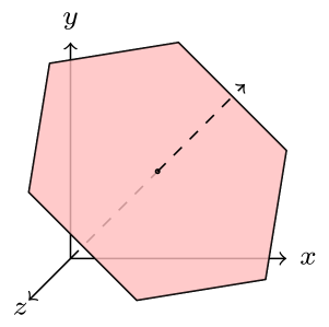
The permutahedron $\mathcal{PH}^{n}$ has $2^{n}-2$ facets, which prevents us from using it in optimization problems directly. (We should note however that the permutahedron is a submodular polyhedron and hence admits efficient algorithms for certain optimization problems.) Relaxations are commonly derived from the set of permutation matrices (the set of $n\times n$ matrices containing zeros and ones, with a single one in each row and column) and its convex hull instead.

Definition 2.2.

The convex hull of the set of $n\times n$ permutation matrices is the Birkhoff polytope $\mathcal{B}^{n}$, which is the set of all doubly-stochastic $n\times n$ matrices:

$$\{X\in\mathbb{R}^{n\times n}\mid X\geq 0,X\mathbf{1}=\mathbf{1},X^{T}\mathbf{1}=\mathbf{1}\}.$$

The Birkhoff polytope has been widely used in the machine learning and computer vision communities for various permutation problems (see for example [2], [3]). The permutahedron can be represented as the projection of the Birkhoff polytope from $\mathbb{R}^{n\times n}$ to $\mathbb{R}^{n}$ by $x_{i}=\sum_{j=1}^{n}j\cdot X_{ij}$. The Birkhoff polytope is sometimes said to be an extended formulation of the permutahedron.

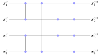
A natural question to ask is whether a more compact extended formulation exists for the permutahedron. Goemans [1] answered this question in the affirmative by constructing an extended formulation with $\Theta(n\log n)$ constraints and variables, which is optimal up to constant factors. His construction is based on sorting networks, a collection of wires and binary comparators that sorts a list of numbers. Figure 1 displays a sorting network on $4$ variables. (See [5] for further more information on sorting networks.)

Figure 1: A bitonic sorting network on 4 variables (left) and the $k$-th comparator (right). The input to the sorting network is on the left and the output is on the right. At each comparator, we take the two input values and sort them such that the smaller value is the one at the top in the output. Sorting takes place progressively as we move from left to right through the network, sorting pairs of values as we encounter comparators.

Given a sorting network on $n$ inputs with $m$ comparators (we will subsequently always use $m$ to refer to the number of comparators), an extended formulation for the permutahedron with $O(m)$ variables and constraints can be constructed as follows [1]. Referring to the notation in the right subfigure in Figure 1, we introduce a set of constraints for each comparator $k=1,2,\dotsc,m$ to indicate the relationships between the two inputs and the two outputs of each comparator:

$$\begin{split}x^{k}_{\text{(in, top)}}+x^{k}_{\text{(in, bottom)}}&=x^{k}_{\text{(out, top)}}+x^{k}_{\text{(out, bottom)}}\\ x^{k}_{\text{(out, top)}}&\leq x^{k}_{\text{(in, top)}}\\ x^{k}_{\text{(out, top)}}&\leq x^{k}_{\text{(in, bottom)}}.\end{split}$$ (1)

Note that these constraints require the sum of the two inputs to be the same as the sum of the two outputs, but the inputs can be closer together than the outputs. Let $x^{\text{in}}_{i}$ and $x^{\text{out}}_{i}$, $i=1,2,\dotsc,n$ denote the $x$ variables corresponding to the $i$th input or output to the entire sorting network, respectively. We introduce the additional constraints

$$x^{\text{out}}_{i}=i,\mbox{ for }i\in[n].$$ (2)

The details of this construction depend on the particular choice of sorting network (see Section 4), but we will refer to it generically as the sorting network polytope $\mathcal{SN}^{n}$. Each element in this polytope can be viewed as a concatenation of two vectors: the subvector associated with the network inputs $x^{\text{in}}=(x^{\text{in}}_{1},x^{\text{in}}_{2},\dotsc,x^{\text{in}}_{n})$, and the rest of the coordinates $x^{\text{rest}}$, which includes all the internal variables as well as the outputs.

Theorem 2.3 (Goemans [1]).

Given the construction above, the set $\{x^{\text{in}}\>|\;(x^{\text{in}},x^{\text{rest}})\in\mathcal{SN}^{n}\}$ is the permutahedron $\mathcal{PH}^{n}$.

In fact, the proof of Theorem 2.3 shows that this construction can be used to describe the convex hull of the permutations of any single vector. Let $v$ be a monotonically-increasing vector. Then, if we replace the constraints (2) with

$$x^{\text{out}}_{i}=v_{i},\mbox{ for }i\in[n]$$ (3)

the set $\{x^{\text{in}}\}$ now corresponds to the convex hull of all permutations of $v$. We include a simple alternative proof of this fact (and by extension Theorem 2.3) in Appendix B.

3 Convex Relaxations of 2-SUM via Sorting Network Polytope

In this section we will briefly describe the seriation problem, and some of the continuous relaxations of the combinatorial 2-SUM problem that can be used to solve this problem.

3.1 The Noiseless Seriation Problem

The term seriation generally refers to data analysis techniques that arrange objects in a linear ordering in a way that fits available information and thus reveals underlying structure of the system [6]. We adopt here the definition of the seriation problem from [4]. Suppose we have $n$ objects arranged along a line, and a similarity function that increases with distance between objects in the line. The similarity matrix is the $n\times n$ matrix whose $(i,j)$ entry is the similarity measure between the $i$th and $j$th objects in the linear arrangement. This similarity matrix is a R-matrix, according to the following definition.

Definition 3.1.

A symmetric matrix $A$ is a Robinson matrix (R-matrix) if for all points $(i,j)$ where $i>j$, we have $A_{ij}\leq\min(A_{(i-1)j},A_{i(j+1)})$. A symmetric matrix $A$ is a pre-R matrix if $\Pi^{T}A\Pi$ is R for some permutation $\Pi$.

In other words, a symmetric matrix is a R-matrix if the entries are nonincreasing as we move away from the diagonal in either the horizontal or vertical direction. The goal of the noiseless seriation problem is to recover the ordering of the variables along the line from the pairwise similarity data, which is equivalent to finding the permutation that recovers an R-matrix from a pre-R-matrix.

The seriation problem was introduced in the archaeology literature [7], and has applications across a wide range of areas including clustering [8], shotgun DNA sequencing [2], and taxonomy [9]. R-matrices are useful in part because of their relation to the consecutive-ones property in a matrix of zeros and ones, where the ones in each column form a contiguous block. A matrix $M$ with the consecutive-ones property gives rise to a R-matrix $MM^{T}$, so the matrix $\Pi^{T}M$ with rows permuted by $\Pi$ leads to a pre-R-matrix $\Pi^{T}MM^{T}\Pi$.

3.2 Noisy Seriation, 2-SUM and Continuous Relaxations

Given a binary symmetric matrix $A$, the 2-SUM problem can be expressed as the following.

$$\min_{\pi\in\mathcal{P}^{n}}\>\> \sum_{i=1}^{n}\sum_{j=1}^{n}A_{ij}(\pi(i)-\pi(j))^{2}.$$ (4)

A slightly simpler but equivalent formulation, defined via the Laplacian $L_{A}=\mbox{diag}(A\mathbf{1})-A$, is

$$\min_{\pi\in\mathcal{P}^{n}}\>\>\pi^{T}L_{A}\pi.$$ (5)

The seriation problem is closely related to the combinatorial 2-SUM problem, and Fogel et al. [2] proved that if $A$ is a pre-$R$-matrix such that each row/column has unique entries, then the solution to the 2-SUM problem also solves the noiseless seriation problem. In another relaxation of the 2-SUM problem, Atkins et al. [4] demonstrate that finding the second smallest eigenvalue, also known as the Fiedler value, solves the noiseless seriation problem. Hence, the 2-SUM problem provides a good model for the noisy seriation problem, where the similarity matrices are close to, but not exactly, pre-R matrices.

The 2-SUM problem is known to be $NP$-hard [10], so we would like to study efficient relaxations. We describe below two continuous relaxations that are computationally practical. (Other relaxations of these problems require solution of semidefinite programs and are intractable in practice for large $n$.)

The spectral formulation of [4] seeks the Fiedler value by searching over the space orthogonal to the vector $\mathbf{1}$, which is the eigenvector that corresponds to the zero eigenvalue. The Fiedler value is the optimal objective value of the following problem:

$$\min_{y\in\mathbb{R}^{n}}\>\>y^{T}L_{A}y\quad\text{such that}\quad y^{T}\mathbf{1}=0,\;\;\|y\|_{2}=1.$$ (6)

This problem is non-convex, but its solution can be found efficiently from an eigenvalue decomposition of $L_{A}$. With Fiedler vector $y$, one can obtain a candidate solution to the 2-SUM problem by picking the permutation $\pi\in\mathcal{P}^{n}$ to have the same ordering as the elements of $y$. Another perspective is given by [11], who prove that the spectral solution minimizes the Frobenius norm of the strongest principal component of a particular derived matrix, and minimizing the Frobenius norm of this matrix is equivalent to minimizing the sums of consecutive zeros between the first and last non-zero entry of a 0-1 matrix. We show in Appendix A that the spectral formulation (6) is a continuous relaxation of the 2-SUM problem (5).

The second relaxation of (5), described by Fogel et al. [2], makes use of the Birkhoff polytope $\mathcal{B}^{n}$. The basic version of the formulation is

$$\min_{\Pi\in\mathcal{B}^{n}}\>\> \pi_{I}^{T}\Pi^{T}L_{A}\Pi\pi_{I},$$ (7)

(recall that $\pi_{I}$ is the identity permutation $(1,2,\dotsc,n)^{T}$), which is a convex quadratic program. Fogel et al. augment and enhance this formulation as follows.

• Introduce a “tiebreaking” constraint $e_{1}^{T}\Pi\pi_{I}+1\leq e^{T}_{n}\Pi\pi_{I}$ to resolve ambiguity about the direction of the ordering, where $e_{k}=(0,\dotsc,0,1,0,\dotsc,0)^{T}$ with the $1$ in position $k$.

• Average over several perturbations of $\pi_{I}$ to improve robustness of the solution.

• Add a penalty to maximize the Frobenius norm of the matrix $\Pi$, which pushes the solution closer to a vertex of the Birkhoff polytope.

• Incorporate additional ordering constraints of the form $x_{i}-x_{j}\leq\delta_{k}$, to exploit prior knowledge about the ordering.

With these modifications, the problem to be solved is

$$\min_{\Pi\in\mathcal{B}^{n}}\>\>\frac{1}{p}\text{Trace}(Y^{T}\Pi^{T}L_{A}\Pi Y)-\frac{\mu}{p}\|P\Pi\|^{2}_{F}\quad\text{such that}\quad D\Pi\pi_{I}\leq\delta,$$ (8)

where each column of $Y\in\mathbb{R}^{n\times p}$ is a slightly perturbed version of a permutation, $\mu$ is the regularization coefficient, the constraint $D\Pi\pi_{I}\leq\delta$ contains the ordering information and tie- breaking constraints, and the operator $P=I-\frac{1}{n}\mathbf{1}\mathbf{1}^{T}$ is the projection of $\Pi$ onto elements orthogonal to the all-ones matrix. The penalization is applied to $\|P\Pi\|^{2}_{F}$ rather than to $\|\Pi\|^{2}_{F}$ directly, thus ensuring that the program remains convex if the regularization factor is sufficiently small (for which a sufficient condition is $\mu<\lambda_{2}(L_{A})\lambda_{1}(YY^{T})$). We will refer to this regularization scheme as the matrix-based regularization, and to the formulation (8) as the matrix-regularized Birkhoff-based convex formulation.

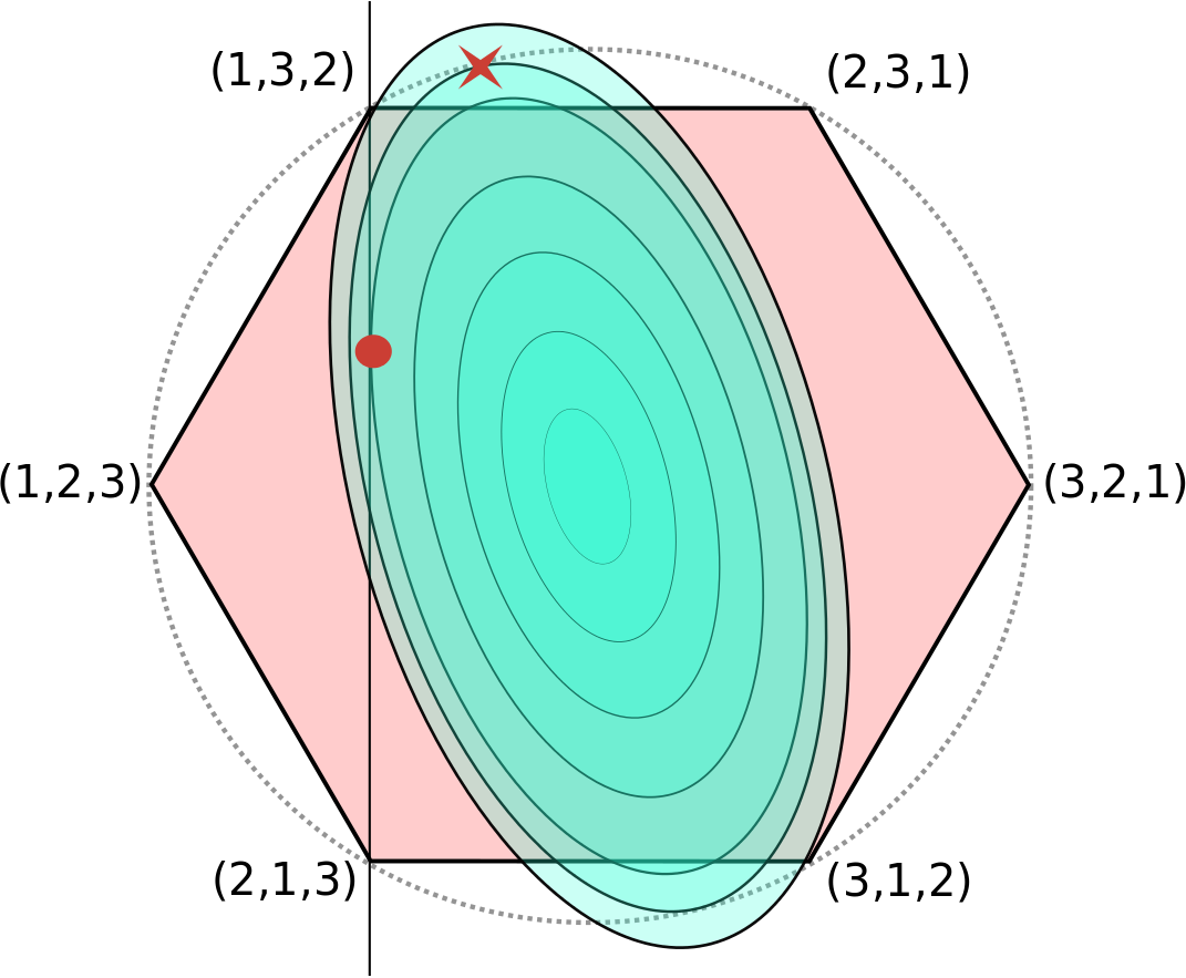
Figure 2 illustrates the permutahedron and the solutions produced by the methods described above. The spectral method returns good solutions when the noise is low and it is computationally efficient since there are many fast algorithms and software for obtaining selected eigenvectors. However, the Birkhoff- based convex formulation can return a solution that is significantly better in situations with high noise or significant additional ordering information. For the rest of this section, we will focus on the convex formulation.

3.3 A Compact Convex Relaxation via the Permutahedron/Sorting Network Polytope and a New Regularization Scheme

Figure 2: A geometric interpretation of spectral and convex formulation solutions on the 3-permutahedron. The left image shows the 3-permutahedron in 3D space and the dashed line shows the eigenvector $\mathbf{1}$ corresponding to the zero eigenvalue. The right image shows the projection of the 3-permutahedron along the trivial eigenvector together with the elliptical level curves of the objective function $y^{T}L_{A}y$. Points on the circumscribed circle have an $\ell_{2}$-norm equal to that of a permutation, and the objective is minimized over this circle at the point denoted by a cross. The vertical line in the right figure enforces the tiebreaking constraint that $1$ must appear before $3$ in the ordering; the red dot indicates the minimizer of the objective over the resulting triangular feasible region. Without the tiebreaking constraint, the minimizer is at the center of the permutahedron.

We consider now a different relaxation forthe 2-SUM problem (5). Taking the convex hull of $\mathcal{P}^{n}$ directly, we obtain

$$\min_{x\in\mathcal{PH}^{n}}\>\> x^{T}L_{A}x.$$ (9)

This is essentially a permutahedron-based version of (7). In fact, two problems are equivalent, except that formulation (9) is more compact when we enforce $x\in\mathcal{PH}$ via the sorting network constraints

$$x\in\{x^{\text{in}}\>|\;(x^{\text{in}},x^{\text{rest}})\in\mathcal{SN}^{n}\},$$

where $\mathcal{SN}^{n}$ incorporates the comparator constraints and the output constraints (2). This formulation can be enhanced and augmented in a similar fashion to (7). The tiebreaking constraint for this formulation can be expressed simply as $x_{1}+1\leq x_{n}$, since $x^{\text{in}}$ consists of the subvector $(x_{1},x_{2},\dotsc,x_{n})$. (In both (9) and (7), having at least one additional constraint is necessary to remove the trivial solution given by the center of the permutahedron or Birkhoff polytope; see Figure 2.) This constraint is the strongest inequality that will not eliminate any permutation (assuming that a permutation and its reverse are equivalent); we include a proof of this fact in Appendix C.

It is also helpful to introduce a penalty to force the solution $x$ to be closer to a permutation, that is, a vertex of the permutahedron. To this end, we introduce a vector-based regularization scheme. The following statement about the norms of permutations is an immediate consequence of strict convexity of norms.

Proposition 3.2.

Let $v\in\mathbb{R}^{n}$, and consider the set $X$ consisting of the convex hull of all permutations of $v$. Then, the points in $X$ with the highest $\ell_{p}$ norm, for $1<p<\infty$, are precisely the permutations of $v$.

It follows that adding a penalty to encourage $\|x\|_{2}$ to be large might improve solution quality. However, directly penalizing the negative of the $2$-norm of $x$ would destroy convexity, since $L_{A}$ has a zero eigenvalue. Instead we penalize $Px$, where $P=I-\frac{1}{n}\mathbf{1}\mathbf{1}^{T}$ projects onto the subspace orthogonal to the trivial eigenvector $\mathbf{1}$. (Note that this projection of the permutahedron still satisfies the assumptions of Proposition 3.2.) When we include a penalty on $\|Px\|_{2}^{2}$ in the formulation (9) along with side constraints $Dx\leq\delta$ on the ordering, we obtain

$$\min_{x\in\mathcal{PH}^{n}}\>\>x^{T}L_{A}x-\mu\|Px\|_{2}^{2}\quad\text{such that}\quad Dx\leq\delta,$$

which can be written as

$$\min_{x\in\mathcal{PH}^{n}}\>\>x^{T}(L_{A}-\mu P)x\quad\text{such that}\quad Dx\leq\delta.$$ (10)

Vector-based regularization decreases all nonzero eigenvalues of $L_{A}$ by the constant $\mu$ while keeping the same eigenvectors. This means that (10) is convex if $\mu$ is smaller than the Fiedler value. This regularization procedure can be thought of as a penalty term corresponding to the constraints in the Fiedler formulation. We will refer to this formulation as the regularized permutahedron-based convex formulation.

Vector-based regularization can also be incorporated into the Birkhoff-based convex formulation. Consider the following corollary of Proposition 3.2 that shows that instead of maximizing the $\|P\Pi\|_{2}^{2}$ term in formulation (8) to force the solution to be closer to a permutation, we could maximize $\|P\Pi Y\|_{2}^{2}$:

Corollary 3.3.

Let $Y\in\mathbb{R}^{n\times p}$ be a matrix where every column has no repeated elements, and consider the set $X=\{P\Pi Y\>|\>\Pi\in\mathcal{B}^{n}\}$ where $P=I-\frac{1}{n}\mathbf{1}\mathbf{1}^{T}$. The elements with the highest Frobenius norm in $X$ are given by the set $\{P\Pi Y\>|\>\Pi\text{ is a permutation matrix}\}$.

The vector-regularized version of (7) with side constraints can be written as follows:

$$\min_{\Pi\in\mathcal{B}^{n}}\>\> \frac{1}{p}\rm{Trace}(Y^{T}\Pi^{T}(L_{A}-\mu P)\Pi Y)\quad\text{such that}\quad D\Pi\pi_{I}\leq\delta.$$ (11)

We refer to this formulation as the vector-regularized Birkhoff-based convex formulation. We note that when we let $Y=\pi_{I}=(1,2,\dotsc,n)^{T}$, the solution of the regularized permutahedron-based convex formulation and the optimal value $\Pi^{\ast}\pi_{I}$ (where $\Pi^{\ast}$ is the solution of (11)) are the same. Hence, we can view the regularized permutahedron-based convex formulation as a compact way of encoding the special case of (11) for which $p=1$.

Vector-based regularization is in some sense more natural than the regularization in (8). It acts directly on the set that we are optimizing over, rather than an expanded set. (Different elements $\Pi_{1}$ and $\Pi_{2}$ of the Birkhoff polytope may yield the same permutation vector: $\Pi_{1}\pi_{I}=\Pi_{2}\pi_{I}$.) In addition, the objective of (11) remains convex provided that $\mu<\lambda_{2}(L_{A})$, a significantly looser constraint that for the matrix-based regularization scheme, allowing for stronger regularization.

The regularized permutahedron-based convex formulation is a convex QP with $O(m)$ variables and constraints, where $m$ is the number of comparators in its sorting network, while the Birkhoff-based one is a convex QP with $O(n^{2})$ variables. In addition, the use of the vector-based regularization scheme in formulations (10) and (11) allows standard convex QP solvers (such as those based on interior-point methods) to be applied to both formulations. The one feature in the Birkhoff-based formulations that the permutahedron-based formulations do not have is the ability to average the solution over multiple vectors by choosing dimension $p>1$ for the matrix $Y\in\mathbb{R}^{n\times p}$. However, our experiments suggested that the best solutions were obtained for $p=1$, so this consideration was not important in practice.

4 Key Implementation Issues

Having described the permutahedron-based convex formulation, we now discuss the important choices to be made in constructing the relaxation and in extracting a suitable permutation from the solution of the relaxation. We also briefly discuss algorithms for solving these formulations, and possible strengthening of the formulations.

Choice of Sorting Network.

There are numerous possible choices of the sorting network, from which the constraints in formulation (10) are derived. The asymptotically most compact option is the AKS sorting network, which contains $\Theta(n\log n)$ comparators. This network was introduced in [12] and subsequently improved by others, but is impractical because of its difficulty of construction and the large constant factor in the complexity expression. We opt instead for more elegant networks with slightly worse asymptotic complexity. Batcher [13] introduced two sorting networks with $\Theta(n\log^{2}n)$ size — the odd-even sorting network and the bitonic sorting network — that are popular and practical. Generation of the constraints that describe the sorting network polytope can be performed with a simple recursive algorithm that runs in $\Theta(n\log^{2}n)$ time. The bitonic sorting network gave good performance in our implementations.

Obtaining Permutations from a Point in the Permutahedron.

Solution of the permutation-based relaxation yields a point $x$ in the permutahedron, but we need techniques to convert this point into a valid permutation, which is a candidate solution for the 2-SUM problem (4). The most obvious recovery technique is to choose this permutation $\pi$ to have the same ordering as the elements of $x$, that is, $x_{i}<x_{j}$ implies $\pi(i)<\pi(j)$, for all $i,j\in\{1,2,\dotsc,n\}$. We could also sample multiple permutations, by applying Gaussian noise to the components of $x$, prior to taking the ordering to produce $\pi$. (In our experiments we added i.i.d. Gaussian noise with variance $0.5$ to each element of $x$ before ordering.) The 2-SUM objective (4) can be evaluated for each permutation so obtained, with the best one being reported as the overall solution. This randomized recovery procedure can be repeated many times, as it is quite inexpensive. Fogel et al. [2] propose a somewhat different permutation sampling procedure for matrices $\Pi$ in the Birkhoff polytope, obtaining a permutation by sorting the vector $\Pi v$, where $v$ is a sorted random vector. We experimented too with decomposition-based methods, in which $x$ is expressed as a convex combination of permutations $\sum_{i=1}^{n+1}\lambda_{i}\pi^{i}$, a decomposition that can be found efficiently using an optimal $O(n^{2})$ algorithm [14]. We evaluated some or all of the spanning permutations by treating the permutations as permutation matrices and applying the sampling procedure from [2], but this approach yielded weaker solutions in general.

Solving the Convex Formulation.

On our test machine using the Gurobi interior point solver, we were able to solve instances of the permutahedron-based convex formulation (10) of size up to around $n=10000$. As in [2], first-order methods can be employed when the scale is larger.

Strengthening Side Structural Information.

The constraint set for our permutation-based relaxation is a polyhedron defined by the sorting network constraints and the side constraints. A much stronger relaxation would be obtained if we could identify the feasible points that correspond to actual permutations, and optimize over the convex hull of these points. (As an example, the set of two constraints $x_{1}+1\leq x_{2}$ and $x_{1}+1\leq x_{3}$ over the 3-permutahedron is satisfied by only two permutations.) However, identifying this convex hull is computationally difficult in general. For example, the convex hull of the set of permutations that satisfy a set of constraints of the form $x_{i}+1\leq x_{j}$ corresponds precisely to the“Single Machine Scheduling Polytope with Scheduling Constraints and Unit Costs”, and since it is $NP$-hard to optimize a linear function over this polytope, computing a linear description is also difficult. Many sets of valid inequalities have been derived for the corresponding scheduling polytope (see [15]), and it will be interesting future work to understand the trade-offs between the tighter solutions that could be obtained by incorporating these valid inequalities and the run time from computing these inequalities.

5 Experiments

We compare the run time and solution quality of algorithms on the two classes of convex formulations — Birkhoff-based and permutahedron-based — with various parameters. Summary results are presented in this section, with additional results appearing in Appendix D.

5.1 Experimental Setup

The experiments were run on an Intel Xeon X5650 (24 cores @ 2.66Ghz) server with 128GB of RAM in MATLAB 7.13, CVX 2.0 ([16],[17]), and Gurobi 5.5 [18]. We tested five formulation-algorithm-implementation variants, as follows.

1. Spectral method using the MATLAB eigs function.

2. Frank-Wolfe algorithm [19] on the Birkhoff-based convex formulations using MATLAB/CVX/Gurobi to solve the linear subproblems.

3. MATLAB/Gurobi on the permutahedron-based convex formulation.

4. MATLAB/Gurobi on the Birkhoff-based convex formulation with $p=1$ (that is, (8) with $Y=\pi_{I}$).

5. Experimental MATLAB code provided to us by the authors of [2] implementing FISTA, for solving the matrix-regularized Birkhoff-based convex formulation (8), with projection steps solved using block coordinate ascent on the dual problem. This is the current state-of-the-art algorithm for large instances of the Birkhoff-based convex formulation; we refer to it as RQPS (for “Regularized QP for Seriation”).

We report run time data using wall clock time reported by Gurobi, and MATLAB timings for RQPS, excluding all preprocessing time.

We used the bitonic sorting network by Batcher [13] for experiments with the permutahedron-based formulation. For consistency between approaches, we used the procedure described in Section 4 for collapsing relaxed solutions to permutations in all cases. For Birkhoff matrices, this means that we applied random Gaussian perturbations (drawn i.i.d. from $N(0,0.5)$) to elements of the vector $\Pi^{*}\pi_{I}$, where $\Pi^{*}$ is the solution of the Birkhoff relaxation. We picked the default parameter settings for the Gurobi interior-point solver except for the convergence tolerance, which is experiment-dependent. We provide more details on algorithm parameters specific to the different variants below.

We vary the number of ordering constraints added for each experiment. Each ordering constraint is of the form $x_{i}+\pi(j)-\pi(i)\leq x_{j}$, where $\pi$ is the (known) permutation that recovers the original matrix, and $i,j\in[n]$ is a pair randomly chosen but satisfying $\pi(j)-\pi(i)>0$.

Besides run time, we used three other metrics to measure performance:

• the 2-SUM objective value of recovered matrix,

• the total number of R-matrix constraints of the form $a_{ij}\leq a_{(i-1)j}$ or $a_{ij}\leq a_{i(j+1)}$ that are violated by the recovered matrix, and

• Kendall’s $\tau$ score to measure how close the permutation obtained is to the permutation that recovers the original matrix.

5.2 Munsingen Dataset

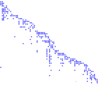
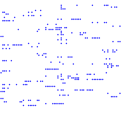
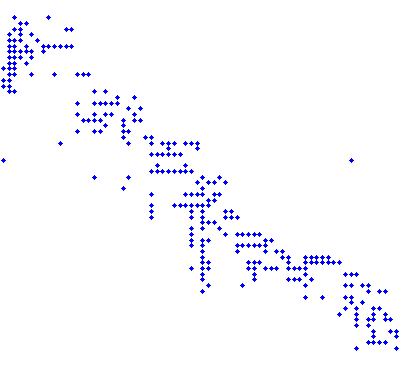
We test the solution quality of the permutahedron-based formulations on a standard problem in the seriation literature drawn from archaeology. The Munsingen dataset, introduced by Hodson [20] and manually re-ordered in [21], was used as a test problem in [2]. It consists of a binary matrix $M$ indicating the presence of each of 70 artifact types on 59 graves, where each artifact is presumed to be associated with a particular time period. The goal is to order the graves by date. We treat this matrix as a noisy consecutive-ones problem and minimize the 2-SUM objective over $MM^{T}$.

Figure 3: Munsingen Dataset. Plot of the Munsingen data matrix $M$ (left), the matrix with rows permuted randomly (center), and the matrix reordered according to the solution of the permutahedron-based convex formulation with 15 randomly chosen ordering constraints (right).

Since we are interested in solution quality (rather than run time performance) for this data set, we used the same algorithm across all the different convex formulations, for consistency: the Frank-Wolfe algorithm with step-size ${2}/{(k+2)}$ (where $k$ is the iteration number), terminating when the relative duality gap is less than one percent. For the regularized permutahedron-based formulation, since it gives the same solution as the vector-regularized Birkhoff-based formulation when $p=1$, we simply apply the Frank-Wolfe algorithm to the latter formulation. We checked that the solutions to the permutahedron-based formulations obtained indirectly in this manner and directly using the Gurobi interior-point solver on the permutahedron-based formulations were similar in quality. We varied the Birkhoff-based convex formulations in three ways. First, we chose the $n\times p$ matrix $Y$ in (8) and (11) to have $p=n$ and $p=4n$ columns (we chose $p\geq n$ to enable application of the matrix-based regularization scheme), with each column in $Y$ chosen by sorting a vector whose entries are independent uniformly distributed random variables in $[0,1]$. (These choices of $p$ and $Y$ are consistent with those used in [2].) Second, we tried both matrix and vector regularization schemes ((8) and (11), respectively). Third, we varied the regularization parameter to be $0\%$, $50\%$ and $90\%$ of the maximum allowed for each respective scheme.

Table 2 displays the results, averaged over ten runs of each variant, each with a different randomly chosen set of 15 ordering constraints. The formulations with vector-based regularization consistently outperform formulations without regularization or with matrix-based regularization, both in the 2-SUM objective and the R-score. The best 2-SUM objectives were obtained for the permutahedron-based formulation. Using $p>1$ in the Birkhoff formulation did not help. The spectral method, which could not make use of any side information about the ordering, did not give competitive results. Results obtained by using 38 ordering constraints (instead of 15) are similar; we report these in Appendix D.

Method	$p$	Reg. Type	Level	2-SUM	Std Err	R-score	Std Err	Kendall’s $\tau$	Std Err
Input				77040	0	289.0	0.0	1.000	0.000
Spectral				77806	0	295.0	0.0	0.755	0.001
Permut.	$-$	none	$-$	72798	6008	306.6	14.9	0.863	0.016
Permut.	$-$	vector	$50\%$	70515	5828	309.4	21.1	0.862	0.017
Permut.	$-$	vector	$90\%$	69336	5422	302.8	22.5	0.867	0.016
Birkhoff	$n$	none	$-$	74111	6966	307.3	33.6	0.859	0.014
Birkhoff	$n$	matrix	$50\%$	73718	6489	306.2	18.8	0.860	0.015
Birkhoff	$n$	matrix	$90\%$	73810	6874	313.0	21.9	0.857	0.014
Birkhoff	$n$	vector	$50\%$	71623	6100	297.6	16.5	0.860	0.019
Birkhoff	$n$	vector	$90\%$	69898	5212	299.9	15.9	0.867	0.016
Birkhoff	$4n$	none	$-$	73257	6713	311.6	16.7	0.856	0.015
Birkhoff	$4n$	matrix	$50\%$	73624	6632	306.3	14.6	0.859	0.017
Birkhoff	$4n$	matrix	$90\%$	73667	6589	305.9	21.5	0.858	0.013
Birkhoff	$4n$	vector	$50\%$	70827	5582	297.4	21.9	0.862	0.009
Birkhoff	$4n$	vector	$90\%$	69490	4927	291.8	15.9	0.868	0.016

Table 2: Munsingen Dataset: Performance with 15 ordering constraints.

5.3 Linear Markov Chain

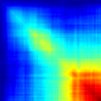
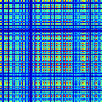
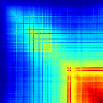
The Markov chain reordering problem [2] involves recovering the ordering of a simple Markov chain with Gaussian noise from disordered samples. The Markov chain consists of random variables $X_{1},X_{2},\dotsc,X_{n}$ such that $X_{i}=bX_{i-1}+\epsilon_{i}$ where $\epsilon_{i}\sim N(0,\sigma^{2})$. A sample covariance matrix taken over multiple independent samples of the Markov chain is used as the similarity matrix in the 2-SUM problem.

Figure 4: Linear Markov Chain covariances. Plot of a covariance matrix corresponding to 50 samples from a length 500 Markov chain (left), the same covariance matrix with rows and columns randomly permuted (center), and the reordered matrix obtained by solving the permutahedron-based convex formulation with 750 randomly chosen ordering constraints (right).

We use this problem for two different comparisons. First, we compare the solution quality and running time of RQPS algorithm of [2] with the Gurobi interior-point solver on the regularized permutahedron-based convex formulation, to demonstrate the performance of the formulation and algorithm introduced in this paper compared with the prior state of the art. Second, we apply Gurobi to both the permutahedron-based and Birkhoff-based formulations with $p=1$, with the goal of discovering which formulation is more efficient in practice.

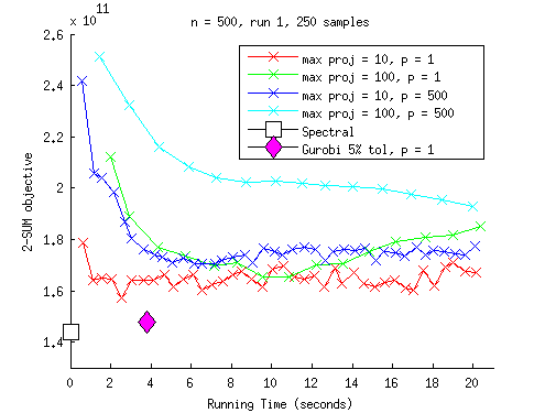
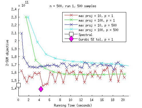
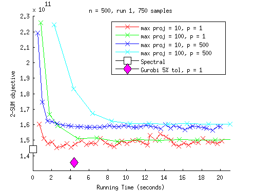
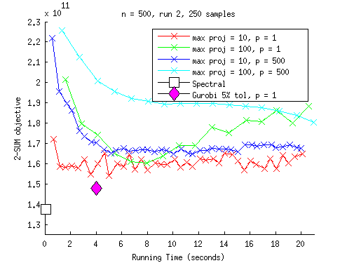
For both sets of experiments, we fixed $b=0.999$ and $\sigma=0.5$ and generate 50 sample sample chains to form a sample covariance matrix. We chose $n\in\{500,2000,5000\}$ to test the scaling of algorithm performance with dimension. For each $n$, we perform 10 independent runs, each based on a different set of samples of the Markov chain (and hence a different sample covariance matrix). Three levels of side constraints were used — $0.5n$, $n$, and $1.5n$ — chosen as described in Subsection 5.1. On initial tests, we observed that the choice of regularization scheme did not significantly affect the performance, so we chose to use vector-based regularization with parameter $\mu=0.9\lambda_{2}(L_{A})$ on all formulations throughout these two sets of experiments.

RQPS and the Permutahedron-Based Formulation.

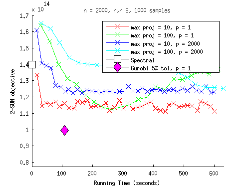
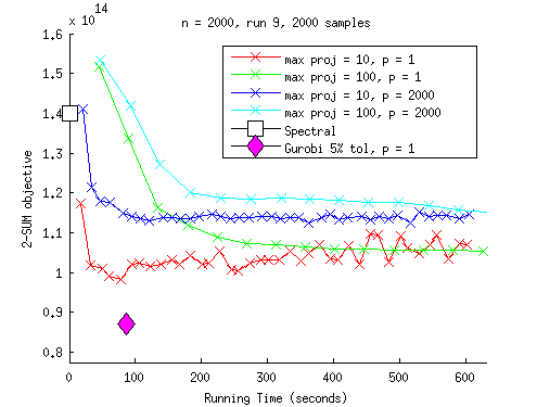
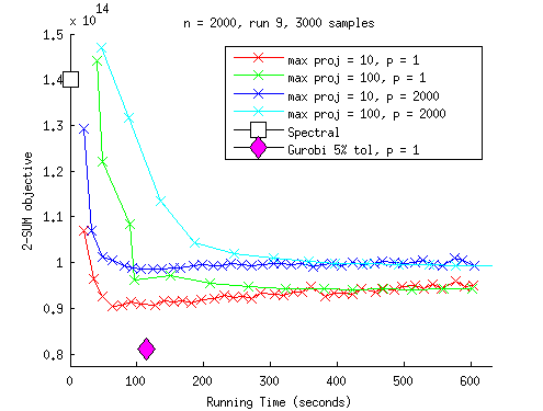
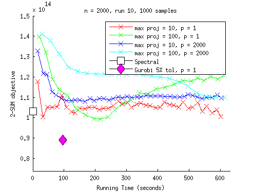
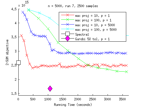
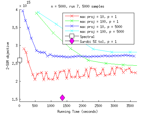
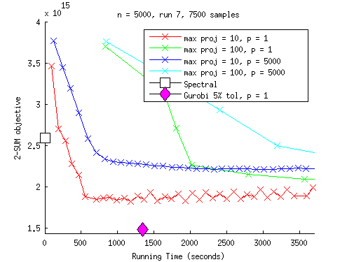
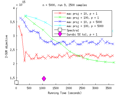
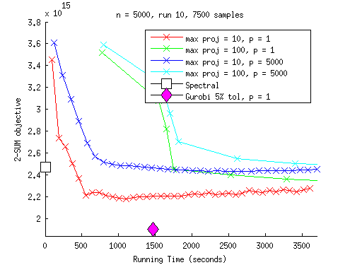
We now compare the RQPS code for the matrix-regularized Birkhoff-based convex formulation (8) to the regularized permutahedron-based convex formulation, solved with Gurobi. We fixed a time limit (which differed according to the value of $n$) and ran the RQPS algorithm until the limit was reached. At fixed time intervals, we query the current solution and sample permutations from that point, using our randomized method described above.

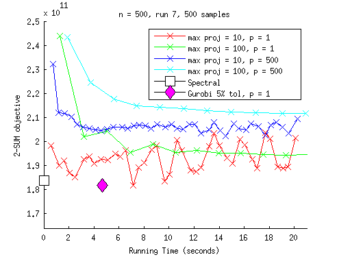
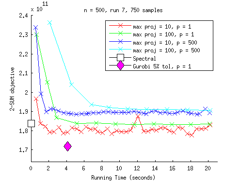
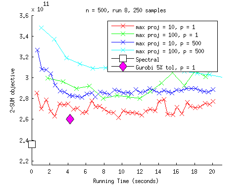
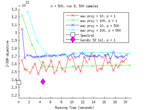
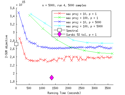
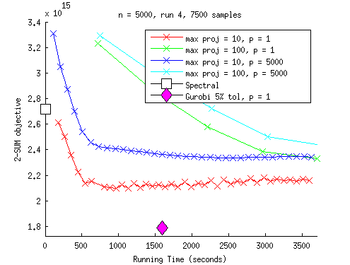
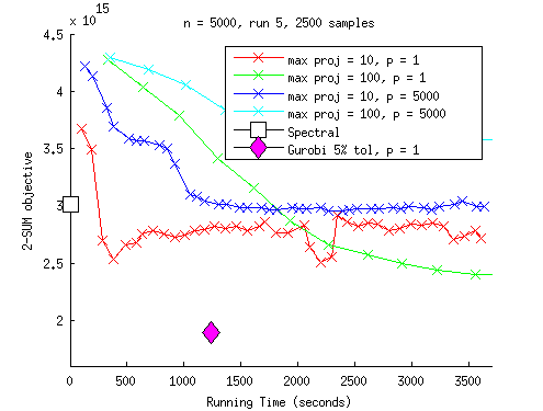
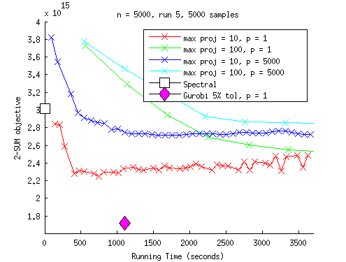
Within the block-coordinate-ascent projection step in the RQPS method, we set a tolerance of 0.001 for the relative primal-dual gap and capped the maximum number of iterations of the primal-dual algorithm to either 10 or 100. We observed that the projection step can be the most costly part of an RQPS iteration, and an imprecise projection can often be sufficient to give good performance (though there is apparently no rigorous theory to guarantee convergence in the presence of an inexact projection calculation). Ten iterations in the projection step usually yielded reasonable performance; the algorithm found a reasonable solution quickly overall, though in some cases the solution quality fluctuates markedly over time. With a 100-iteration limit in the projection subproblem, there is less fluctuation in 2-SUM value over the course of iterations, but the time per FISTA iteration increases significantly. (A cap of fewer than 10 yields erratic convergence behavior, while greater than 100 is too slow.)

In applying Gurobi’s interior-point solver to the permutahedron-based formulation, we set a relative tolerance of 5% and applied the randomized procedure described above to recover a permutation from the final point. We observed that use of a loose tolerance does not usually degrade the solution quality by more than a percent or two over results obtained with a tight tolerance, and avoids numerical instabilities in the interior-point methods.

$n=500$, run 3

$n=2000$, run 7

$n=5000$, run 8

Figure 5: Linear Markov Chain Example. Plot of 2-SUM objective over time (in seconds) for $n\in\{500,2000,5000\}$. The red, green, blue, and cyan curves represent performance of the RQPS code for varying values $p$ and the cap on the maximum number of iterations for the projection step. The white square represents the spectral solution, and the magenta diamond represents the solution returned by Gurobi for the permutahedron-based formulation. The horizontal axis in each graph is positioned at the 2-SUM objective of the identity permutation on the sample covariance matrix.

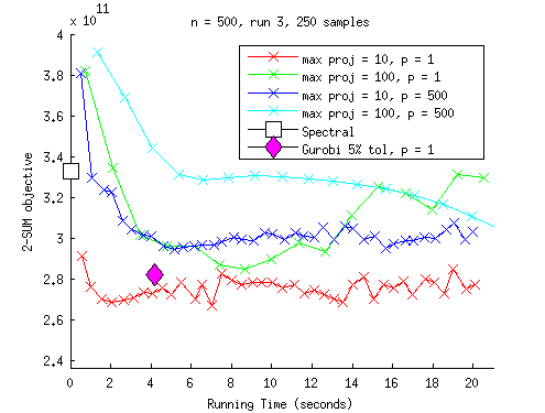
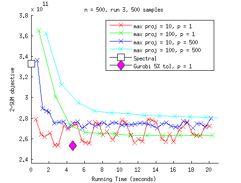
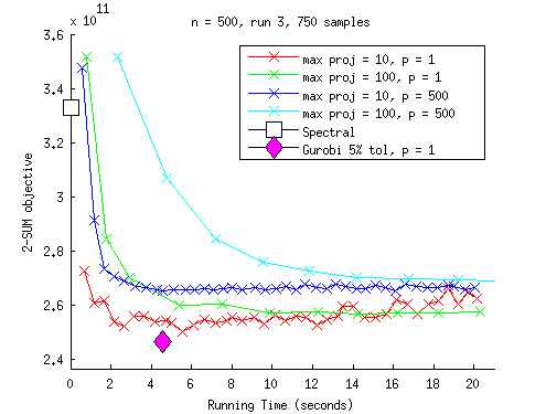
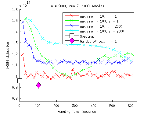
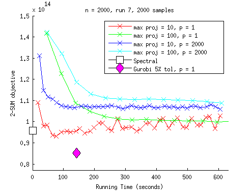
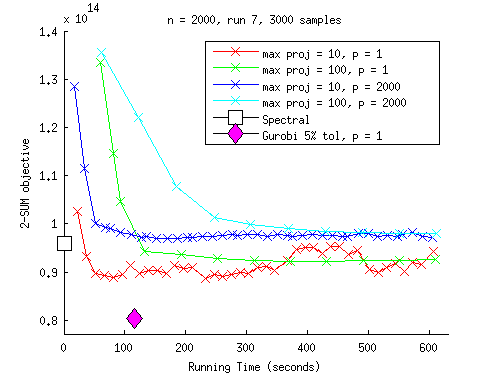
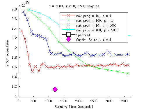
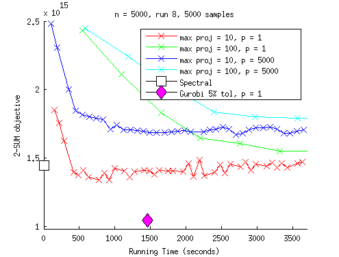
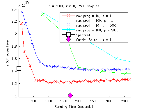
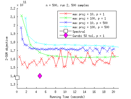
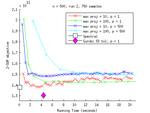
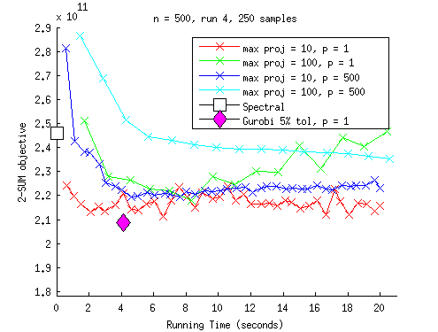
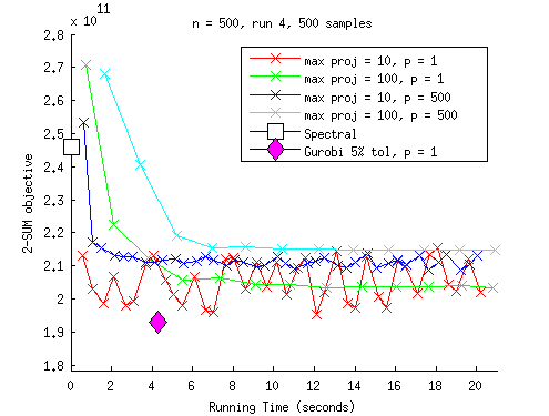
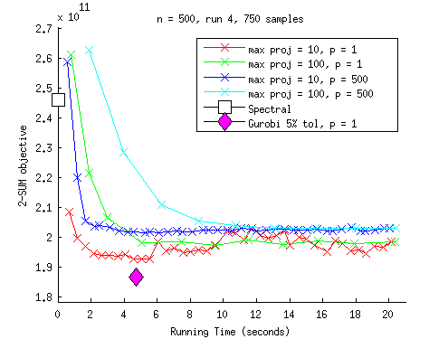
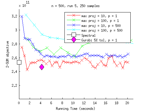
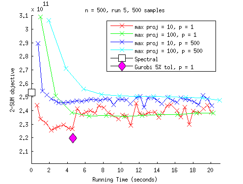
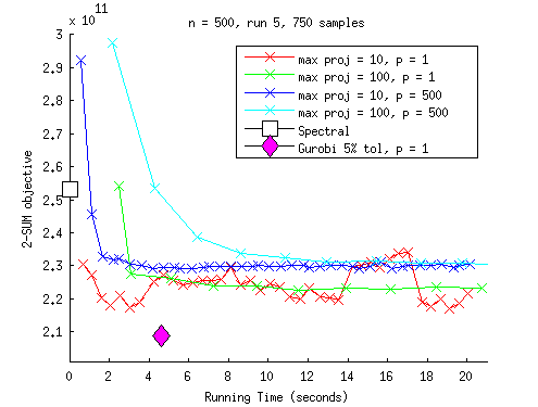
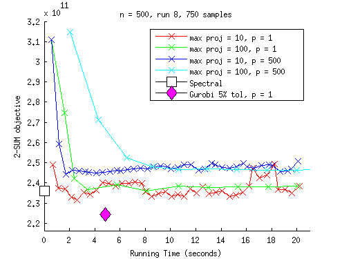
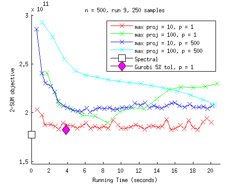
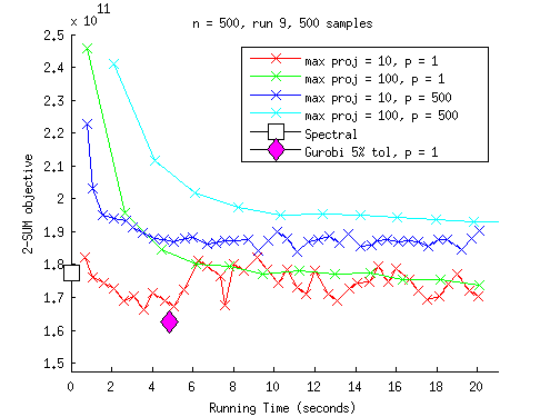
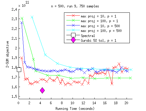
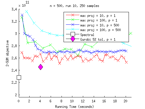
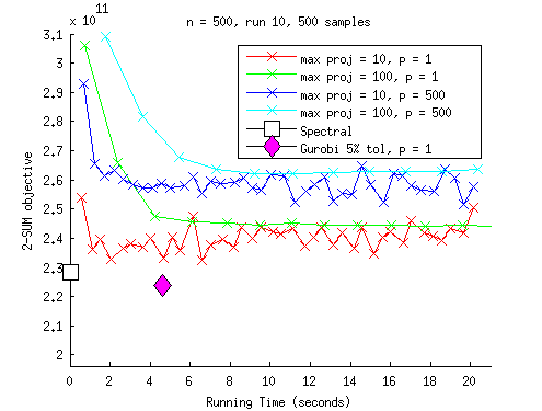
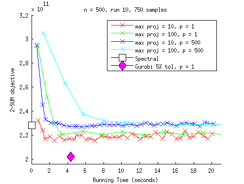
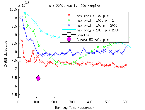
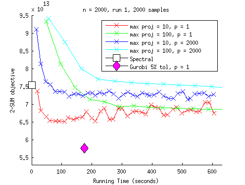
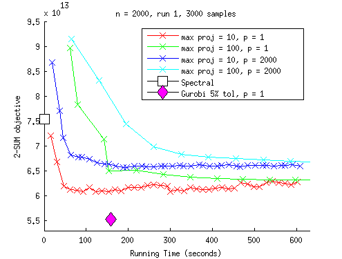
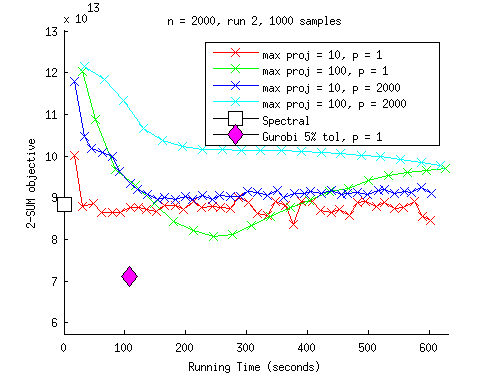
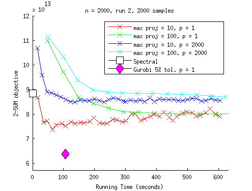
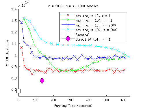
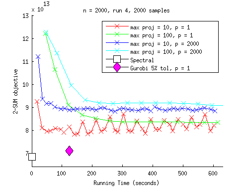
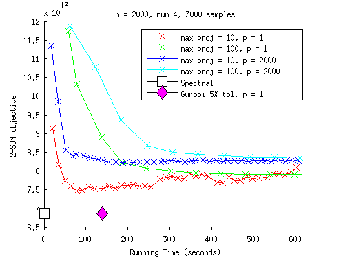
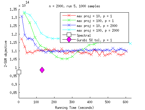
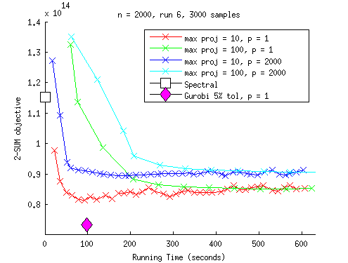
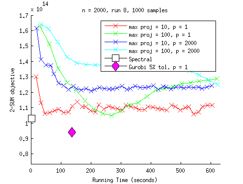
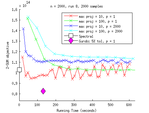
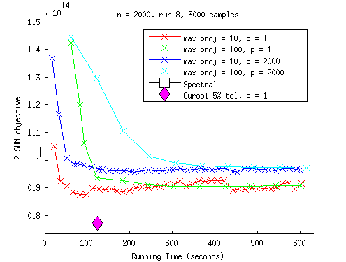
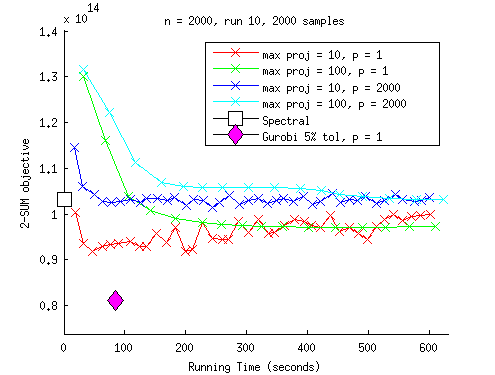
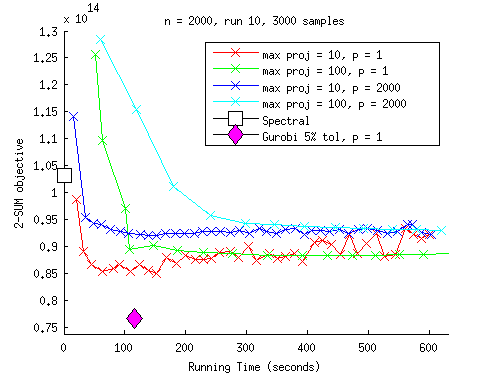
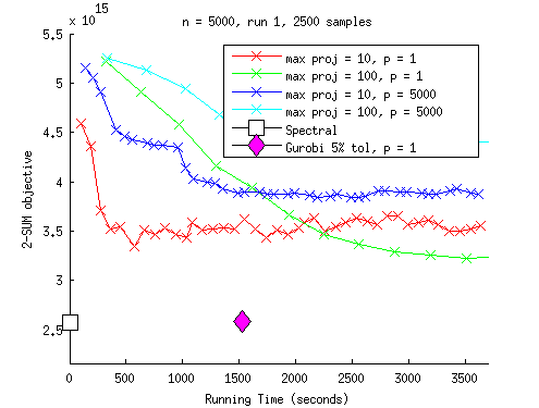
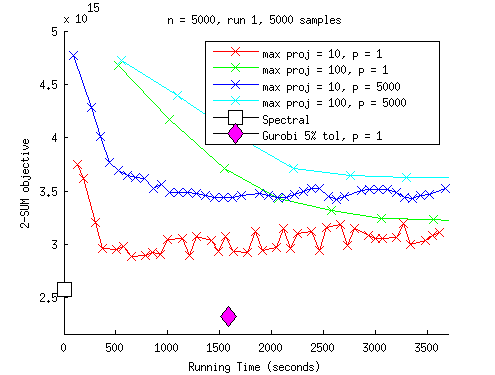
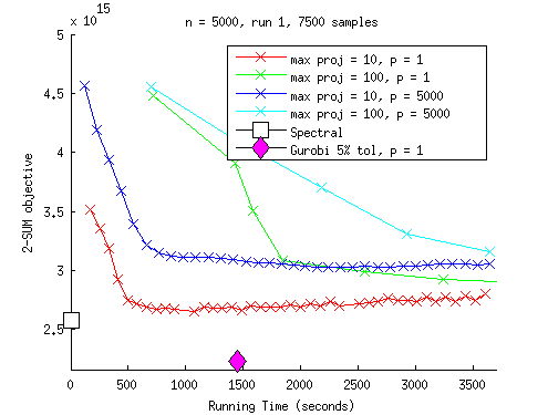
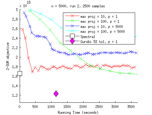
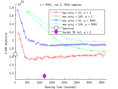
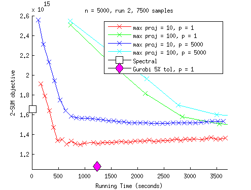
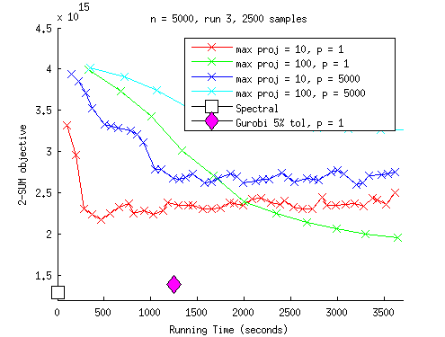
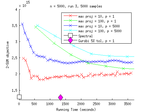
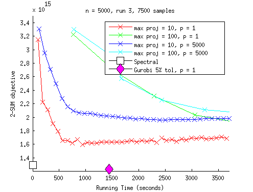
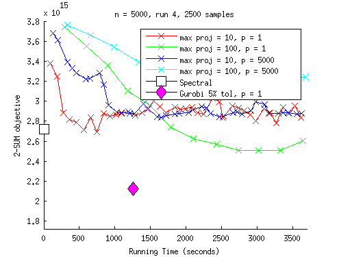
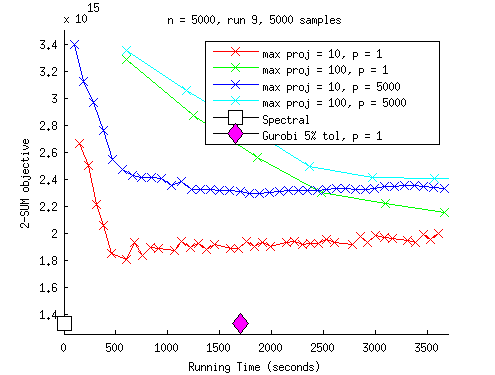
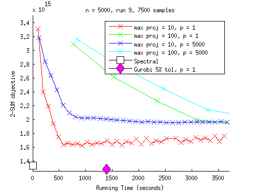
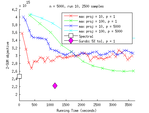
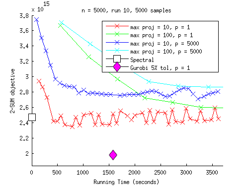
Figure 5 shows results corresponding to the three different values of $n$, each row of plots corresponding to $n=500$, $n=2000$, and $n=5000$. For each $n$, we choose the run (out of ten) that shows the best results for RQPS relative to the interior-point algorithm for the regularized permutahedron-based formulation, and report remaining runs in Appendix D. Each column of plots corresponds to a different number of side constraints: $n/2$, $n$, and $3n/2$, as discussed above. We report results for four different variants of RQPS, differing according to the cap on iterations in the projection step and to the value of $p$ in (8), as follows:

• maximum 10 iterations in the projection, with $p=1$;

• maximum 100 iterations in the projection, with $p=1$;

• maximum 10 iterations in the projection, with $p=n$;

• maximum 100 iterations in the projection, with $p=n$.

We also report results obtained for the permutahedron-based formulation and for the spectral formulation (which cannot use side constraints).

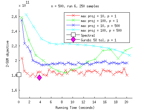
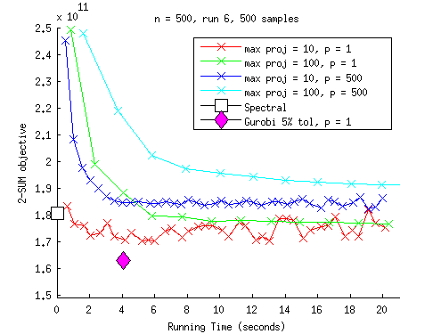
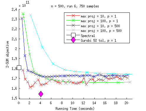
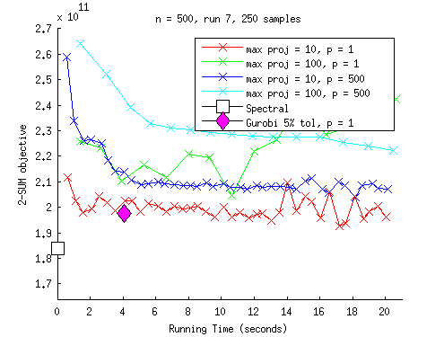
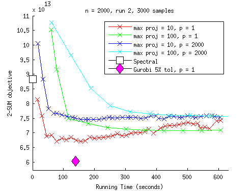
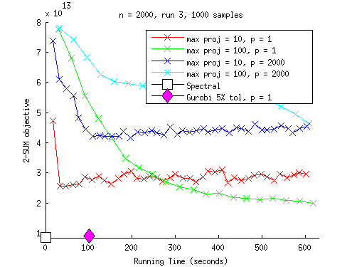
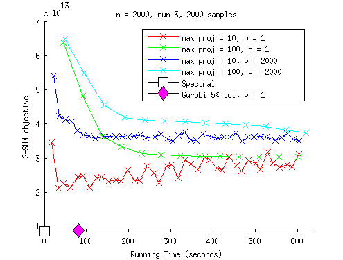
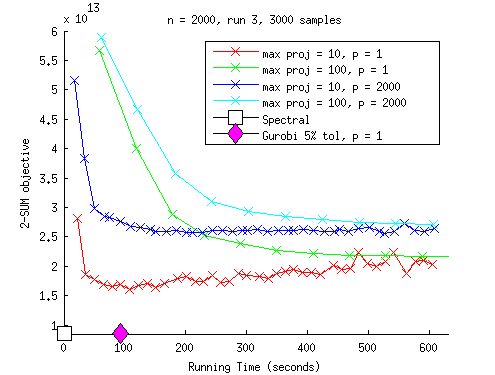
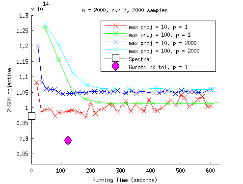
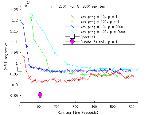
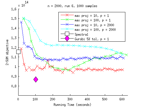
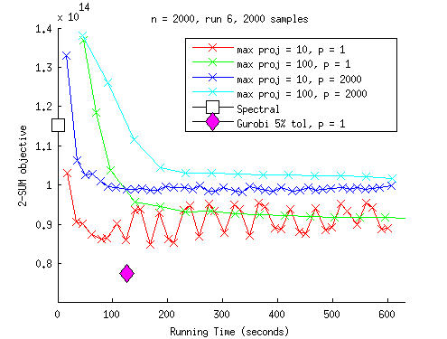
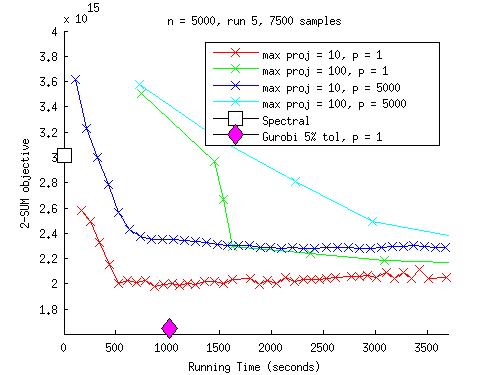
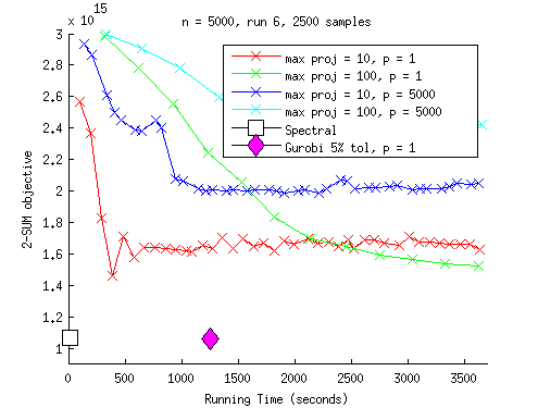
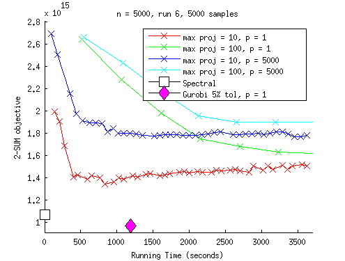
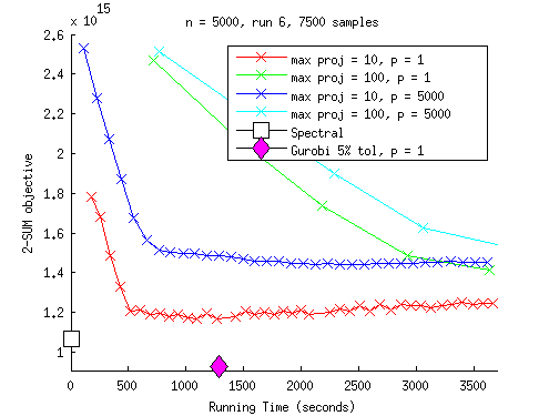
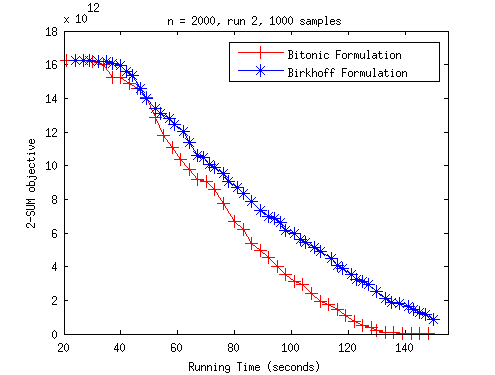
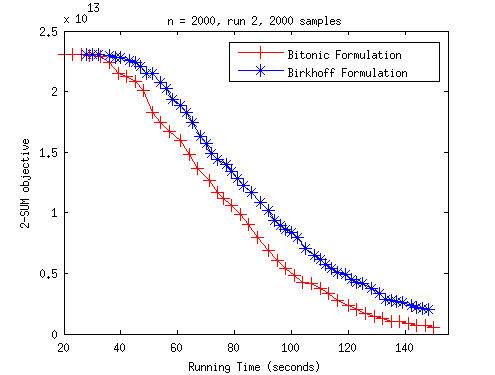
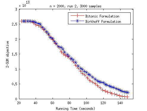
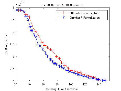
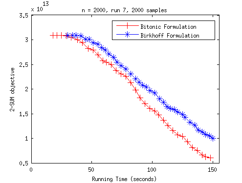
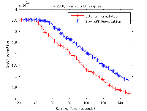
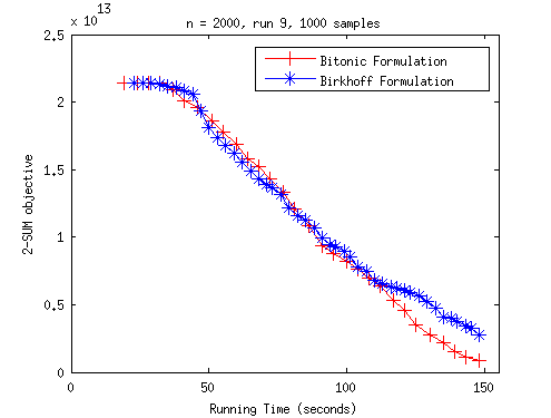
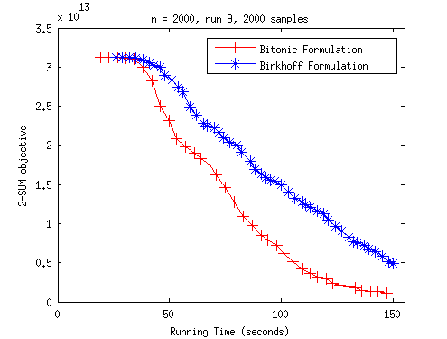
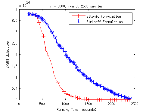
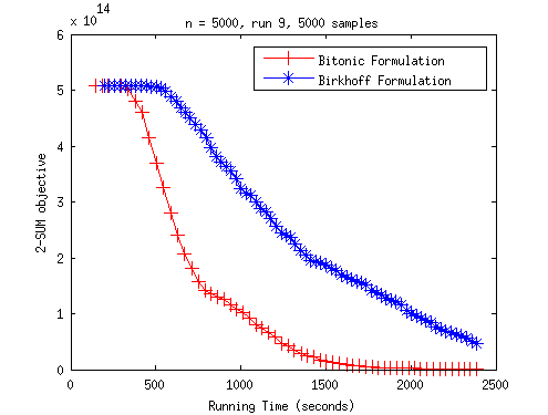
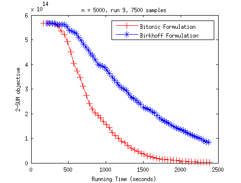
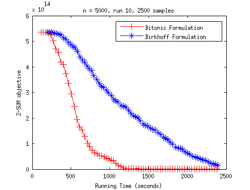
The plots show the quality of solution produced by the various methods (as measured by the 2-SUM objective on the vertical axis) vs run time (horizontal axis). For RQPS, with a cap of $10$ iterations within each projection step, the objective tends to descend to a certain level rapidly, but then proceeds to fluctuate around that level for the rest of the running time, or sometimes gets worse. For a cap of 100 iterations, there is less fluctuation in 2-SUM value, but it takes some time to produce a solution as good as the previous case. Contrary to experience reported in [2], values of $p$ greater than $1$ do not seem to help; our runs for $p=n$ plateaued at higher values of the 2-SUM objective than those with $p=1$.

We now compare the RQPS results to those obtained with the regularized permutahedron-based formulation. In most cases, the latter formulation gives a better solution value, but there are occasional exceptions to this rule. For example, in the third run for $n=500$ (the top left plot in Figure 5), one variant of RQPS converges to a solution that is significantly better. Despite its very fast run times, the spectral method does not yield solutions of competitive quality, due to not being able to make use of the side constraint information.

Direct Comparison of Birkhoff and Permutahedron Formulations

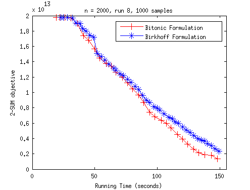
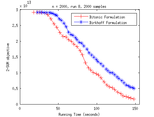
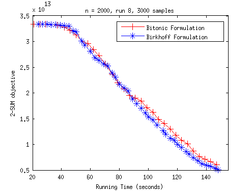
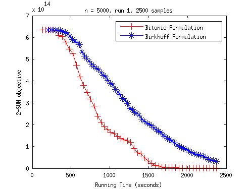
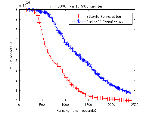
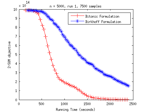
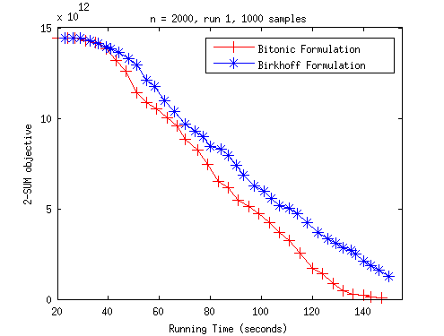
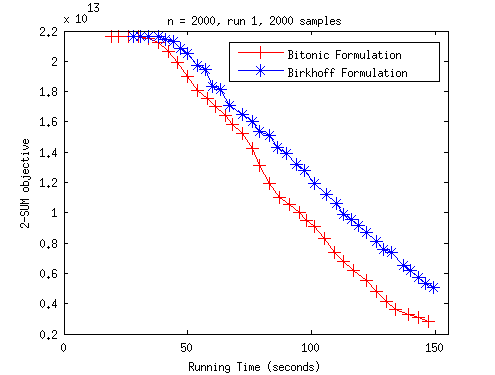
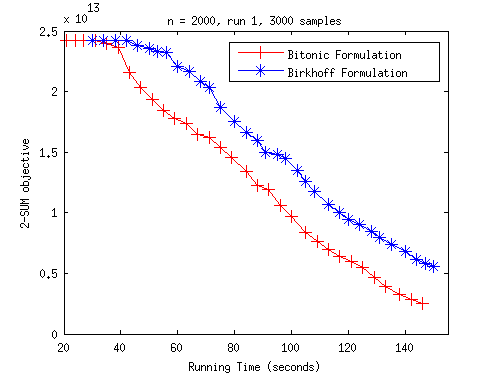
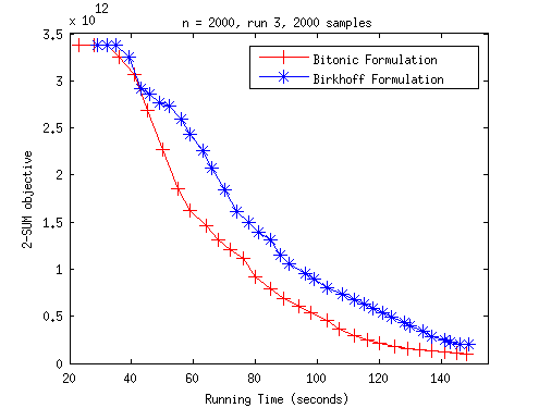
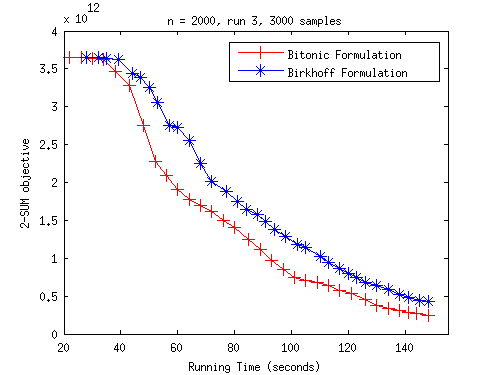
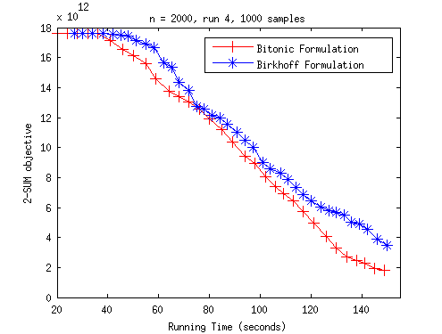
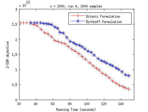
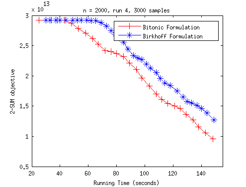
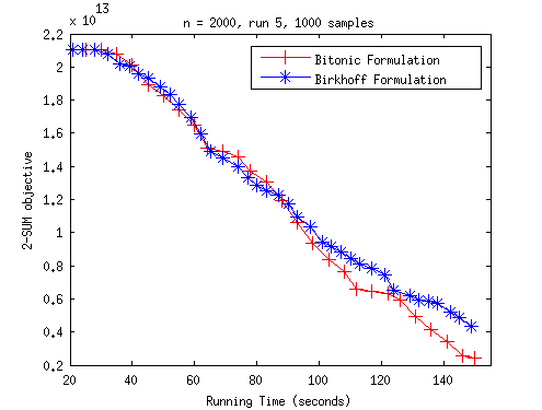
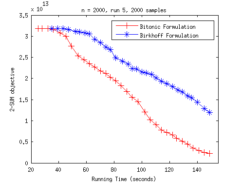
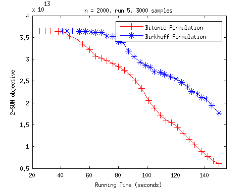
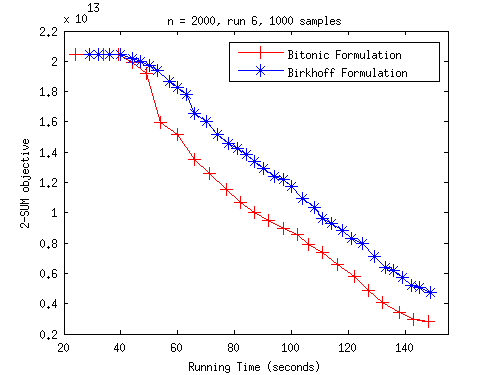
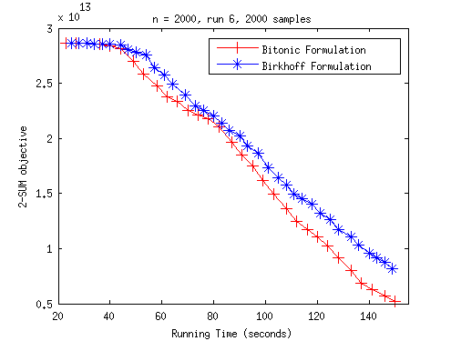
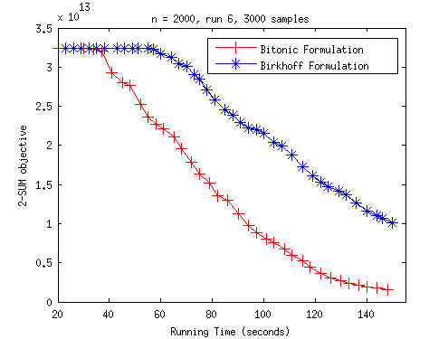
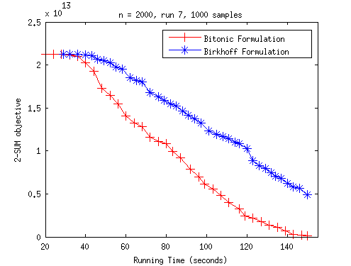
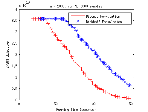
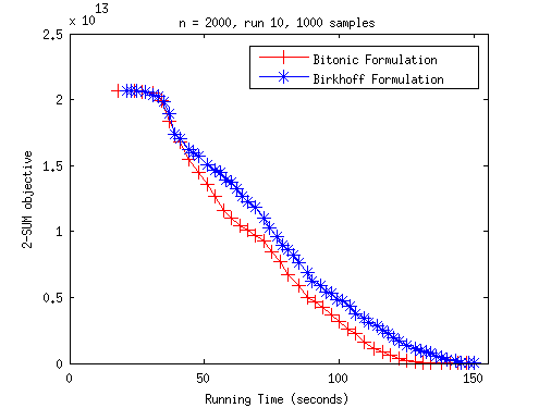
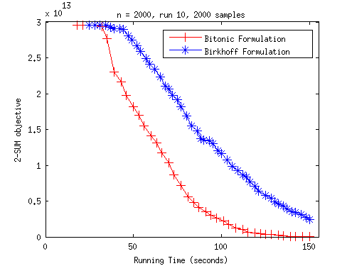
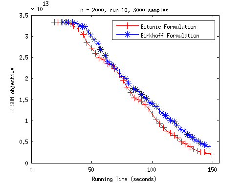
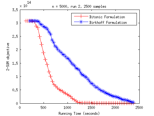
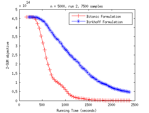
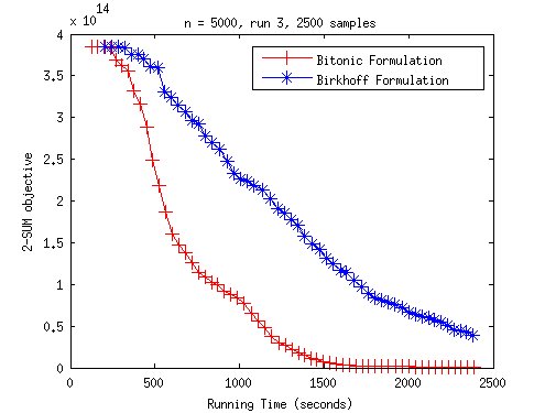
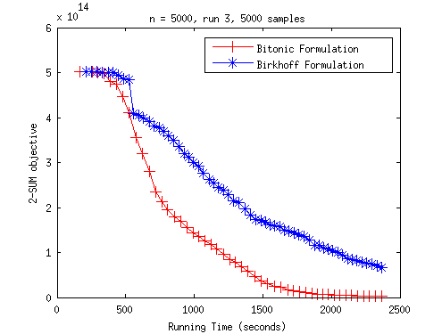
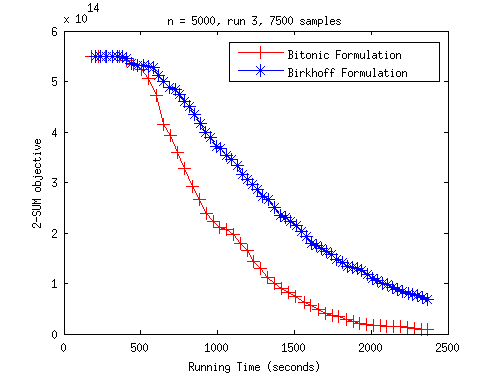
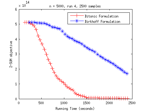
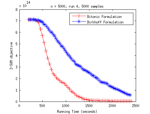
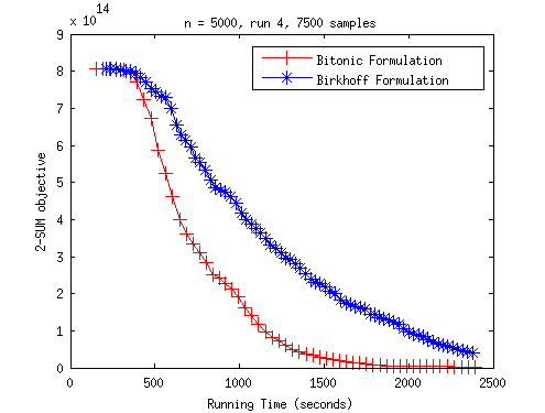
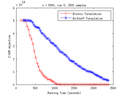
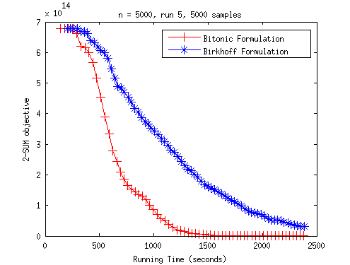
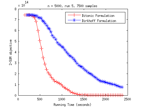
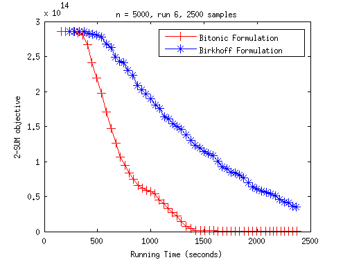
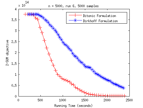
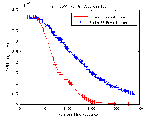
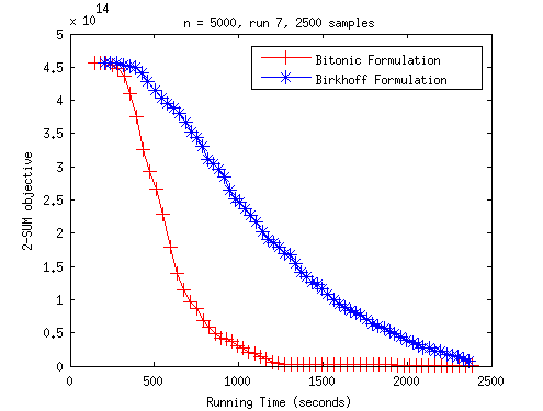
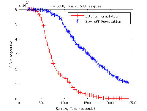
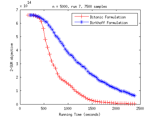
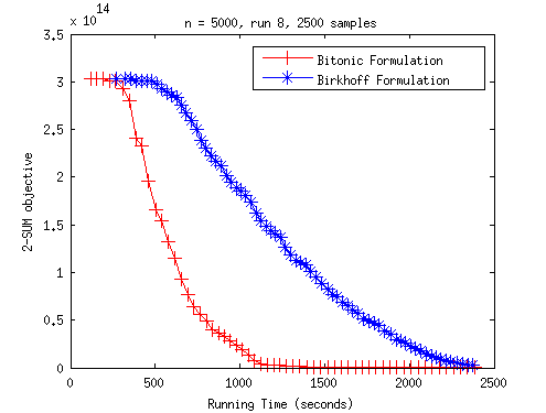
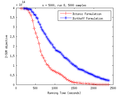
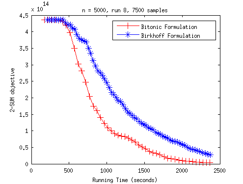
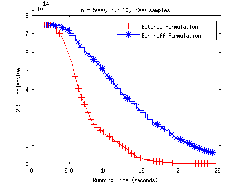
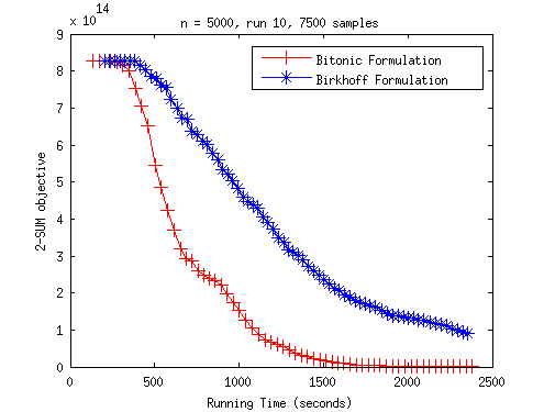
For the second set of experiments, we compare the convergence rate of the objective value in the Gurobi interior-point solver applied to two equivalent formulations: the vector-regularized Birkhoff-based convex formulation (11) with $p=1$ and the regularized permutahedron-based convex formulation (10). For each choice of input matrix and sampled ordering information, we first solved each formulation to within a 0.1% tolerance (or until reaching a preset time limit) to obtain a baseline objective $\overline{v}$, then ran the Gurobi interior-point method for each formulation. At each iteration, we plot the difference between the primal objective and $\overline{v}$.

$n=2000$, run 8

$n=5000$, run 1

Figure 6: Linear Markov Chain Example. Plot of the difference of the 2-SUM objective from the baseline objective over time (in seconds) for $n\in\{2000,5000\}$. The red curve represents performance of the permutahedron-based formulation; the blue curve represents the performance of the Birkhoff-based formulation. For each value of $n$, we display the best run (out of ten) for the Birkhoff-based formulation.

Figure 6 shows the results for the best run (out of ten) for the Birkhoff-based formulation relative to the permutahedron-based formulation for $n\in\{2000,5000\}$. (Results for $n=500$ are omitted because we could not obtain accurate timing information for short run times.) For $n=2000$, the permutahedron-based formulation usually converges faster, but for the best run for the Birkhoff-based formulation they have similar performance. However, once we scale up to $n=5000$, the permutahedron-based formulation converges significantly faster in all tests.

Our comparisons show that the permutahedron-based formulation tends to yield better solutions in faster times than Birkhoff-based formulations, regardless of which algorithm is used to solve the latter. The advantage of the permutahedron-based formulation is more pronounced when $n$ is large.

5.4 Additional Empirical Observations

We omitted results from the convex formulations when there was no sampled information, since we have observed that this could lead to inconsistent results. In general, we have noticed that in many of those cases the value of the obtained point on the permutahedron lies in a narrow range, and the randomness inherent in the procedure of sampling a permutation may be a major factor in determining the solution quality.

6 Conclusions and Future Work

In this paper, we bring Goemans’ compact description of the permutahedron into the area of convex optimization, showing that it can be used to construct a convex relaxation of the 2-SUM problem problem as introduced by [2] — an optimization in which the variable is a permutation of $n$ objects. Enhancements introduced in the Birkhoff-based formulations can also be applied to the permutahedron-based formulations. We introduce a new, simpler regularization scheme that gives solutions of the relaxation that can be turned into better candidate solutions for the underlying problem. We also introduce a simple randomized scheme for recovering permutations from solutions of the relaxation. Empirical results show that the regularized permutahedron-based formulation gives the best objective values and converges more rapidly than algorithms applied to the Birkhoff-based formulation when $n$ is large. Given that the permutation-based formulation requires only $\Theta(n\log^{2}n)$ variables and constraints, whereas the Birkhoff-based formulation requires $\Theta(n^{2})$, the advantage of the permutahedron-based scheme should continue to grow as $n$ increases.

We hope that this paper spurs further interest in using sorting networks in the context of other more general classes of permutation problems, such as graph matching or ranking. A direct adaptation of this approach is inadequate, since the permutahedron does not uniquely describe a convex combination of permutations, which is how the Birkhoff polytope is used in many such problems. However, when the permutation problem has a solution in the Birkhoff polytope that is close to an actual permutation, we should expect that the loss of information when projecting this point in the Birkhoff polytope to the permutahedron to be insignificant.

7 Acknowledgements

We thank Okan Akalin and Taedong Kim for helpful comments and suggestions for the experiments. We thank the anonymous referees for feedback that improved the paper’s presentation. We also thank the authors of [2] for sharing their experimental code, and Fajwal Fogel for helpful discussions.

Lim’s work on this project was supported in part by NSF Awards DMS-0914524 and DMS-1216318, and a grant from ExxonMobil. Wright’s work was supported in part by NSF Award DMS-1216318, ONR Award N00014-13-1-0129, DOE Award DE-SC0002283, AFOSR Award FA9550-13-1-0138, and Subcontract 3F-30222 from Argonne National Laboratory.

Appendix A The Spectral Formulation is a Continuous Relaxation of the 2-SUM Problem

Consider the following problem:

$$\min_{x\in\Re^{n}}\>\>x^{T}L_{A}x\quad\text{such that}\quad x^{T}\mathbf{1}=\frac{n(n+1)}{2},\;\;\|x\|^{2}_{2}=\frac{n(n+1)(2n+1)}{6}.$$ (12)

The set of permutations lies in the hyperplane defined by $x^{T}\mathbf{1}={n(n+1)}/{2}$, and each permutation has a $\ell_{2}$-norm of $\sqrt{n(n+1)(2n+1)/6}$. Hence, formulation (12) is a continuous relaxation of the 2-SUM problem (5). If we shift variables to $z:=x-(({n+1})/{2})\mathbf{1}$, the objective becomes

$$x^{T}L_{A}x=z^{T}L_{A}z+\left(\frac{n+1}{2}\right)^{2}\mathbf{1}^{T}L_{A}\mathbf{1}=z^{T}L_{A}z$$

which follows from the fact that the $L_{A}\mathbf{1}=0$. Note that $z^{T}\mathbf{1}=0$ if and only if

$$x^{T}\mathbf{1}=z^{T}\mathbf{1}+n\frac{n+1}{2}=\frac{n(n+1)}{2},$$

and if $z^{T}\mathbf{1}=0$ holds, then $\|z\|^{2}_{2}=\frac{n(n+1)(2n+1)}{6}-\frac{n(n+1)^{2}}{4}$ if and only if

$$\|x\|^{2}_{2}=\left\|z+\frac{n+1}{2}\mathbf{1}\right\|^{2}_{2}=\|z\|^{2}_{2}+2\cdot z^{T}\mathbf{1}+\frac{n(n+1)^{2}}{2}=\|z\|^{2}_{2}+0+\frac{n(n+1)^{2}}{4}=\frac{n(n+1)(2n+1)}{6}.$$

This shows that formulations (6) and (12) are equivalent up to constant factors, and hence (6) is also a continuous relaxation of (5), up to a constant factor.

Appendix B Proofs for Sections 2 and 3

We provide an alternative proof of Theorem 2.3 and provide proofs of the results stated when we introduced the convex relaxations.

B.1 Alternative Proof of Theorem 2.3

Suppose we have a monotonically-increasing vector $v$ and the set $P_{v}$, the convex hull of all permutations of $v$. Let $\mathcal{SN}_{v}^{n}$ denote the sorting network polytope associated with the vector $v$ by replacing the variables on the output wires by $x^{\text{out}}_{i}=v_{i}$ for all $i\in[n]$.

Proof.

The sorting network ensures that the permutahedron $\mathcal{P}_{v}^{n}$ is contained in $\{x^{\text{in}}\>|\;(x^{\text{in}},x^{\text{rest}})\in\mathcal{SN}_{v}^{n}\}$, and since the set is convex it also contains the convex hull of the permutahedron.

We will now prove the other containment. Let $y=(y_{1},\dotsc,y_{n})$ denote the values on the $n$ wires before a particular comparator $k$, and let $z=(z_{1},\dotsc,z_{n})$ denote the values after. It suffices to prove that if $z$ is in the convex hull of the permutahedron, then so is $y$. Let $a$ and $b$ denote the indices of the wires that are part of comparator $k$. Let $z^{\prime}$ be the point obtained by swapping the values of the $a$th and $b$th coordinates. We have $z\in\mathcal{P}_{v}^{n}$ by assumption, and $z^{\prime}\in\mathcal{P}^{n}_{v}$ since the permutahedron is invariant under swapping of coordinates. The constraints (1) ensure that $y$ is a convex combination of points $z$ and $z^{\prime}$, hence $y\in\mathcal{P}_{v}^{n}$. ∎

B.2 Proof of Proposition 3.2

Proof.

Every permutation of the vector $v$ has the same $\ell_{p}$-norm, and since the $\ell_{p}$-norm is strictly-convex for $1<p<\infty$ and $X$ is defined by the convex hull of permutations of $v$, the proposition holds. ∎

B.3 Proof of Corollary 3.3

Proof.

Let $y_{1},y_{2},\dotsc,y_{p}$ denote the columns of the matrix $Y$. Since

$$\|P\Pi Y\|_{2}=\sqrt{\sum_{i=1}^{n}\sum_{j=1}^{p}(P\Pi Y)_{ij}^{2}}=\sqrt{\sum_{j=1}^{p}\|P\Pi y_{j}\|^{2}},$$

it suffices to pick the matrix $\Pi$ to maximize each $\|P\Pi y_{j}\|$ term. Since $P\Pi=\Pi P$, each set $\{P\Pi y_{j}\>|\>\Pi\in\mathcal{B}^{n}\}=\{\Pi Py_{j}\>|\>\Pi\in\mathcal{B}^{n}\}$ is the convex hull of all permutations of $Py_{j}$. This means that by proposition 3.2, the norm $\|P\Pi y_{j}|$ is maximized by choosing $\Pi$ such that $\Pi Py_{j}$ is a permutation of $Py_{j}$. The entries in $y_{j}$ are unique so $\Pi$ has to be a permutation matrix. ∎

Appendix C Characterizing the $\mathcal{PH}^{n}\cap\{x\in\mathbb{R}^{n}\>|\>x_{1}+1\leq x_{n}\}$ polytope

In this section, we will provide a characterization of the permutahedron with tiebreaking constraint that will later be useful in developing first-order algorithms. This characterization will provide the intuition for why, in the absence of other structured information, the tiebreaking constraint is the “best” single constraint one can add to the permutahedron for the convex relaxations we study.

C.1 Preliminaries

A simple characterization of the points in the permutahedron of the permutahedron from the theory of majorization (see [22]) will be useful for our proof.

Lemma C.1.

A point $x\in\mathbb{R}^{n}$ is in $\mathcal{PH}^{n}$ if and only if the point $z$ obtained by sorting the coordinate-wise values of $x$ in descending order satisfies the equations

$$\sum_{i=1}^{k}z_{i}\leq\sum_{i=1}^{k}(n+1-i)$$ (13)

for all $k\in[n]$ and

$$\sum_{i=1}^{n}z_{i}=\frac{n(n+1)}{2}.$$ (14)

Proof.

Any $x\in\mathcal{PH}^{n}$ immediately satisfies the conditions on $z$ since the set of equations (13) and (14) represent a subset of the equations defining the permutahedron. As for the other direction, consider $x$ and the corresponding $z$ that satisfies equations (13) and (14). Then, given $S\subseteq[n]$ we have

$$\sum_{i\in S}x_{i}\leq\sum_{i=1}^{|S|}z_{i}\leq\sum_{i=1}^{|S|}(n+1-i).$$

Since this holds for all subsets $S$, $x$ has to be in the permutahedron. ∎

C.2 Characterization and Proof

The permutahedron with tiebreaking constraint can be shown to be the convex hull of all permutations $\pi$ such that $\pi(1)<\pi(n)$, which is equivalent to the following theorem:

Theorem C.2.

Every extreme point of $\mathcal{PH}^{n}\cap\{x\in\mathbb{R}^{n}\>|\>x_{1}+1\leq x_{n}\}$ is a permutation.

This implies that the tiebreaking constraint is the single strongest inequality that one can introduce without cutting off any permutations. We can optimize linear functions efficiently over this set [23].

To prove the theorem we only need to study the facet introduced by adding the tiebreaking constraint $x_{1}+1\leq x_{n}$. We will show that every point on $T=\mathcal{PH}^{n}\cap\{x\in\mathbb{R}^{n}\>|\>x_{1}+1=x_{n}\}$ that is not a permutation can be expressed as a convex combination of two other points in the set. In other words, all the extreme points on the facet $T$ are permutations.

Consider $x\in T$ and let $z$ be the sorted vector such that $z_{k}$ is the $k$-th largest element in $x$. Let $\pi$ be a permutation where $z_{\pi(k)}=x_{k}$. Since $x_{n}$ is larger than $x_{1}$, this means that $\pi(n)<\pi(1)$. Let $s\in\mathbb{R}^{n}$ denote the slack in the inequalities in equation (13), given by

$$s_{k}=\sum_{i=1}^{k}(n+1-i)-\sum_{i=1}^{k}z_{i}$$

If $x$ is not a permutation, then there must exist indices $a$, $b$ such that $s_{a}$ is the first non-zero value in $s$ and $s_{b}$ is the first zero value after $s_{a}$. Note that we have

$$z_{k} =n+1-k\text{ for }k<a,$$ (15)

$$z_{a} =n+1-a-s_{a}<n+1-a,$$ (16)

$$z_{b} =n+1-b+s_{b-1}>n+1-b.$$ (17)

We will now show that $x$ can be expressed as a convex combination of two other points. There are three main cases to consider. The first (and simplest) case is when $\pi(1)\neq b$ and $\pi(n)\neq a$, and the second case is when $\pi(n)=a$, and the third case is when $\pi(1)=b$. (The case where $\pi(1)=a$ or $\pi(n)=b$ does not occur.)

Lemma C.3.

$\pi(1)\neq a$ and $\pi(n)\neq b$.

Proof.

Suppose for contradiction that $\pi(1)=a$. Then, there is some index $c<a$ such that $\pi(n)=c$, which gives us

$$\sum_{i=1}^{a}z_{i}=\sum_{i=1}^{c}z_{i}+\sum_{i=c+1}^{a}z_{i} \geq\left(\sum_{i=1}^{c}(n+1-i)\right)+\sum_{i=c+1}^{a}z_{i}$$

$$\geq\left(\sum_{i=1}^{c}(n+1-i)\right)+(a-c)\cdot(n+1-c-1)$$

$$\geq\sum_{i=1}^{a}(n+1-i)$$

where the first inequality follows from (15), and the second inequality from $z_{c}\geq z_{k}\geq z_{a}=z_{c}-1$ for $c<k<a$. This is a contradiction because it implies that either the slack term $s_{a}$ is zero or that $x$ is not in the permutahedron.

The argument for $\pi(n)\neq b$ is similar. If $\pi(n)=b$, there is some index $c>b$ such that $\pi(1)=c$. We have

$$\sum_{i=1}^{b+1}z_{i}=\sum_{i=1}^{b}z_{i}+z_{b+1} \geq\left(\sum_{i=1}^{b}(n+1-i)\right)+z_{b+1}$$

$$\geq\left(\sum_{i=1}^{b}(n+1-i)\right)+n+1-b+s_{b-1}-1$$

$$>\sum_{i=1}^{b+1}(n+1-i)$$

where the second inequality follows from $z_{b}\geq z_{b+1}\geq z_{c}=z_{b}-1$ and (17), and the third inequality from the fact that the slack $s_{b-1}$ is greater than zero. This is a contradiction since it implies $x$ is not in the permutahedron. ∎

Before we proceed with the case-by-case analysis, we will first introduce a small $\delta$ term that will help us define two points such that their convex combination gives us $x$. Consider the terms $\Delta_{k}=z_{k}-z_{k+1}$ and pick $\delta>0$ such that

$$\delta<\min\left(\{\Delta_{k}\>|\>k\in[n-1],\Delta_{k}>0\}\cup\{s_{i}\>|\>a\leq i<b\}\right).$$

This choice of $\delta$ is small enough to allow us to take advantage of the ‘wiggle-room’ that the slack affords us.

We will tackle each of the two cases in separate lemmas.

Lemma C.4.

If $\pi(1)\neq b$ and $\pi(n)\neq a$, then the points $v^{+}$ and $v^{-}$ given by

$$v^{+}_{k}=\begin{cases}x_{k}+\delta&\mbox{if }\pi(k)=a\\ x_{k}-\delta&\mbox{if }\pi(k)=b\\ x_{k}&\mbox{otherwise }\end{cases}\qquad\text{and}\qquad v^{-}_{k}=\begin{cases}x_{k}-\delta&\mbox{if }\pi(k)=a\\ x_{k}+\delta&\mbox{if }\pi(k)=b\\ x_{k}&\mbox{otherwise }\end{cases}$$

satisfy $0.5v^{+}+0.5v^{-}=x$ and are in the permutahedron.

Proof.

Suppose $\pi(1)\neq b$ and $\pi(n)\neq a$. By Lemma C.3, we know that $\pi(1),\pi(n)\notin\{a,b\}$. The vectors $v^{+}$ and $v^{-}$ exploit this fact by adding or subtracting the $\delta$ term from these coordinates.

To show that $v^{+}$ is in the polytope, consider the vector $z^{+}$ which is the vector $v^{+}$ sorted in descending order. We will prove that for $z^{+}$ every coordinate $k\in[n]$ satisfies equation (13). The choice of $\delta$ ensures that the order between elements that are not equal in $z$ is preserved in $z^{+}$. Then, for $k$ such that $a\leq k<b$, we have

$$\sum_{i=1}z^{+}_{i}\leq\delta+\sum_{i=1}^{k}z_{i}\leq s_{k}+\sum_{i=1}^{k}z_{i}=\sum_{i=1}^{k}(n+1-i).$$

For $k\geq b$, $\sum_{i=1}^{k}z^{+}_{i}=\sum_{i=1}^{k}z_{i}$, so all that remains is to show that equation (13) holds for $k<a$. We can prove this by noting that $z^{+}_{k}=z_{k}$ for $k<a$. From the slack terms, we know that $z_{a-1}=n-a+2$ and $z_{a}<n-a+1<z_{a-1}$. By the choice of $\delta$, we know that $z_{a}+\delta<z_{a-1}$, hence the ordering of the first $a$ terms remains the same in $z^{+}$ and $z$ and the desired equality holds. The proof for $v^{-}$ is similar. ∎

The construction of points $v^{+}$ and $v^{-}$ for the case where $\pi(n)=a$ will require a little more care since we can no longer directly add $\delta$ to $z_{a}$ and have the point remain in the polytope.

Lemma C.5.

If $\pi(n)=a$, then $x$ is not an extreme point.

Proof.

Let $c=\pi(1)$. An argument similar to the $\pi(n)\neq b$ part of Lemma C.3 shows that the indices satisfy $c\leq b$. Now we divide the proof into two different cases. For the case where $a<c<b$, we construct the points $v^{+}$ and $v^{-}$ where

$$v^{+}_{k}=\begin{cases}x_{k}+\delta/2&\mbox{if }k\in\{1,n\}\\ x_{k}-\delta&\mbox{if }\pi(k)=b\\ x_{k}&\mbox{otherwise }\end{cases}\qquad\text{and}\qquad v^{-}_{k}=\begin{cases}x_{k}-\delta/2&\mbox{if }k\in\{1,n\}\\ x_{k}+\delta&\mbox{if }\pi(k)=b\\ x_{k}&\mbox{otherwise }\end{cases}.$$

For the $c=b$ case, we have $a<b-1$ otherwise $a=b-1$ and $z_{b}=z_{a}-1$, so $s_{a}=s_{b}>0$ which is not possible due to the definition of $b$. Then, we can define $v^{+}$ and $v^{-}$ as follows:

$$v^{+}_{k}=\begin{cases}x_{k}+\delta/2&\mbox{if }k\in\{1,n\}\\ x_{k}-\delta&\mbox{if }\pi(k)=b-1\\ x_{k}&\mbox{otherwise }\end{cases}\qquad\text{and}\qquad v^{-}_{k}=\begin{cases}x_{k}-\delta/2&\mbox{if }k\in\{1,n\}\\ x_{k}+\delta&\mbox{if }\pi(k)=b-1\\ x_{k}&\mbox{otherwise }\end{cases}.$$

The same argument for Lemma C.4 applies to both of these cases. ∎

The proof for the final case is similar to the second case, with the roles of $a$ and $b$ swapped. We omit it.

Lemma C.6.

If $\pi(1)=b$, then $x$ is not an extreme point.

Putting the lemmas together concludes the proof of the theorem. The result in this section can be slightly generalized. Instead of the tiebreaking constraint $x_{1}+1\leq x_{n}$, one can replace the constraint with $x_{i}+k\leq x_{j}$ for any $k\in[n-1]$ and $i,j\in[n]$ and prove that every extreme point of the resulting polytope is a permutation.

On the other hand, this result only applies to the permutahedron, and not the convex hull of the permutations of an arbitrary point. This proof relies on the fact that the difference between every two adjacent elements on the sorted permutation vector is a fixed constant. Given a vector $x\in\mathbb{R}^{n}$ ($n>3$) where this does not hold and the polytope formed by taking the convex hull of all permutations of $x$, every non-trivial single inequality that retains all permutations with $x_{1}<x_{n}$ would create an extreme point that is not a permutation.

Appendix D Additional Experiment Details

We include all the results for the Munsingen experiment and the linear Markov chain experiment.

Method	$p$	Reg. Type	Level	2-SUM	Std Err	R-score	Std Err	Kendall’s $\tau$	Std Err
Input				77040	0	289.0	0.0	1.000	0.000
Spectral				77806	0	295.0	0.0	0.755	0.001
Permut.	$-$	none	$-$	72105	2908	318.0	17.7	0.891	0.015
Permut.	$-$	vector	50%	70683	2670	316.6	12.2	0.892	0.015
Permut.	$-$	vector	90%	70075	2836	311.2	13.6	0.892	0.013
Birkhoff	$n$	none	$-$	72726	3389	317.3	24.4	0.891	0.011
Birkhoff	$n$	matrix	50%	73198	3433	314.2	14.2	0.889	0.014
Birkhoff	$n$	matrix	90%	72824	3334	322.1	15.3	0.889	0.016
Birkhoff	$n$	vector	50%	71570	2878	309.3	16.5	0.890	0.015
Birkhoff	$n$	vector	90%	70999	2964	306.4	14.4	0.892	0.010
Birkhoff	$4n$	none	$-$	73534	3556	317.0	20.0	0.889	0.011
Birkhoff	$4n$	matrix	50%	73177	3225	321.6	21.9	0.889	0.012
Birkhoff	$4n$	matrix	90%	74590	4532	319.2	14.9	0.885	0.012
Birkhoff	$4n$	vector	50%	72440	2917	317.7	17.9	0.891	0.010
Birkhoff	$4n$	vector	90%	71127	2805	305.8	16.6	0.891	0.011

Table 3: Munsingen dataset — Performance with 38 ordering constraints.

Figure 7: Linear Markov Chain — Plot of 2-SUM objective over time for $n=500$ for runs 1 to 5.

Figure 8: Linear Markov Chain — Plot of 2-SUM objective over time for $n=500$ for runs 6 to 10.

Figure 9: Linear Markov Chain — Plot of 2-SUM objective over time for $n=2000$ for runs 1 to 5.

Figure 10: Linear Markov Chain — Plot of 2-SUM objective over time for $n=2000$ for runs 6 to 10.

Figure 11: Linear Markov Chain — Plot of 2-SUM objective over time for $n=5000$ for runs 1 to 5.

Figure 12: Linear Markov Chain — Plot of 2-SUM objective over time for $n=5000$ for runs 6 to 10.

Figure 13: Linear Markov Chain — Plot of the difference of the 2-SUM objective from the baseline objective over time for $n=2000$ for runs 1 to 5.

Figure 14: Linear Markov Chain — Plot of the difference of the 2-SUM objective from the baseline objective over time for $n=2000$ for runs 6 to 10.

Figure 15: Linear Markov Chain — Plot of the difference of the 2-SUM objective from the baseline objective over time for $n=5000$ for runs 1 to 5.

Figure 16: Linear Markov Chain — Plot of the difference of the 2-SUM objective from the baseline objective over time for $n=5000$ for runs 6 to 10.

References

- [1] M. Goemans, “Smallest compact formulation for the permutahedron,” Working Paper, 2010.
- [2] F. Fogel, R. Jenatton, F. Bach, and A. D’Aspremont, “Convex Relaxations for Permutation Problems,” in Advances in Neural Information Processing Systems, 2013, pp. 1016–1024.
- [3] M. Fiori, P. Sprechmann, J. Vogelstein, P. Muse, and G. Sapiro, “Robust Multimodal Graph Matching: Sparse Coding Meets Graph Matching,” in Advances in Neural Information Processing Systems, 2013, pp. 127–135.
- [4] J. E. Atkins, E. G. Boman, and B. Hendrickson, “A Spectral Algorithm for Seriation and the Consecutive Ones Problem,” SIAM Journal on Computing, vol. 28, no. 1, pp. 297–310, Jan. 1998.
- [5] T. H. Cormen, C. Stein, R. L. Rivest, and C. E. Leiserson, Introduction to Algorithms, 2nd ed. McGraw-Hill Higher Education, 2001.
- [6] I. Liiv, “Seriation and matrix reordering methods: An historical overview,” Statistical Analysis and Data Mining, vol. 3, no. 2, pp. 70–91, 2010.
- [7] W. S. Robinson, “A Method for Chronologically Ordering Archaeological Deposits,” American Antiquity, vol. 16, no. 4, p. 293, Apr. 1951.
- [8] C. Ding and X. He, “Linearized cluster assignment via spectral ordering,” in Twenty-first international conference on Machine learning - ICML ’04. New York, New York, USA: ACM Press, Jul. 2004, p. 30.
- [9] R. Sokal and P. H. A. Sneath, Principles of Numerical Taxonomy. London: W. H. Freeman, 1963.
- [10] A. George and A. Pothen, “An Analysis of Spectral Envelope Reduction via Quadratic Assignment Problems,” SIAM Journal on Matrix Analysis and Applications, vol. 18, no. 3, pp. 706–732, Jul. 1997.
- [11] N. Vuokko, “Consecutive ones property and spectral ordering,” in 10th SIAM International Conference on Data Mining (SDM ’10), 2010, pp. 350–360.
- [12] M. Ajtai, J. Komlós, and E. Szemerédi, “An O(n log n) sorting network,” in Proceedings of the fifteenth annual ACM symposium on Theory of computing - STOC ’83. New York, New York, USA: ACM Press, Dec. 1983, pp. 1–9.
- [13] K. E. Batcher, “Sorting networks and their applications,” in Proceedings of the April 30–May 2, 1968, spring joint computer conference on - AFIPS ’68 (Spring). New York, New York, USA: ACM Press, Apr. 1968, p. 307.
- [14] S. Yasutake, K. Hatano, S. Kijima, E. Takimoto, and M. Takeda, “Online linear optimization over permutations,” in Algorithms and Computation, ser. Lecture Notes in Computer Science, T. Asano, S.-i. Nakano, Y. Okamoto, and O. Watanabe, Eds. Springer Berlin Heidelberg, 2011, vol. 7074, pp. 534–543.
- [15] M. Queyranne and A. S. Schulz, “Polyhedral approaches to machine scheduling,” Department of Mathematics, Technical University of Berlin, Tech. Rep. Technical Report 408/1994, 1994.
- [16] M. Grant and S. Boyd, “CVX: Matlab software for disciplined convex programming, version 2.0,” http://cvxr.com/cvx, Aug. 2012.
- [17] ——, “Graph implementations for nonsmooth convex programs,” in Recent Advances in Learning and Control, ser. Lecture Notes in Control and Information Sciences, V. Blondel, S. Boyd, and H. Kimura, Eds. Springer-Verlag Limited, 2008, pp. 95–110, http://stanford.edu/~boyd/graph_dcp.html.
- [18] Gurobi Optimizer Reference Manual, Gurobi Optimization, Inc., 2014. [Online]. Available: http://www.gurobi.com
- [19] M. Frank and P. Wolfe, “An algorithm for quadratic programming,” Naval Research Logistics Quarterly, vol. 3, no. 1-2, pp. 95–110, 1956.
- [20] F. Hodson, The La Tène Cemetery at Münsingen-Rain: Catalogue and relative chronology, ser. Acta Bernensia. Stämpfli, 1968.
- [21] D. G. Kendall, “Abundance matrices and seriation in archaeology,” Probability Theory and Related Fields, vol. 17, no. 2, pp. 104–112, Jun. 1971.
- [22] A. W. Marshall, I. Olkin, and B. C. Arnold, Inequalities: Theory of Majorization and Its Applications: Theory of Majorization and Its Applications. Springer, 2011.
- [23] E. Lawler, Sequencing Jobs to Minimize Total Weighted Completion Time Subject to Precedence Constraints, ser. Annals of Discrete Mathematics. Elsevier, 1978, vol. 2.