Abstract

Harald Skarke
Institut für Theoretische Physik, Technische Universität Wien
Wiedner Hauptstraße 8–10, 1040 Wien, Austria

ABSTRACT

1 Introduction

While data from cosmological observations are reaching unprecedented levels of precision, their interpretation still rests on the pioneering works of Friedmann, Lemaitre, Robertson and Walker (FLRW), who assumed perfect spatial homogeneity. This basic framework is refined by linear perturbation theory which describes small deviations from uniformity very well, thereby providing an excellent description of the physics of the early universe. In the present cosmological era the deviations from homogeneity are definitely not small. Therefore a clear procedure for relating measurements from an inhomogeneous universe to some FLRW model is needed. The fact that this is an open question that needs to be addressed properly was recognized already in Ref. [4], where it was called the “fitting problem”. This issue became particularly important with the advent of data [5, 6] that, if interpreted in terms of a naive application of the FLRW models, indicated the presence of a positive cosmological constant $\Lambda$ or a dark energy with similar characteristics. While the majority of cosmologists seem to agree that this is indeed the correct interpretation, there have also been many alternative proposals (see e.g. [7] for a review). This question was also the motivation for the present work (as for its predecessor [8]), which introduces a formalism that transcends perturbation theory in its treatment of inhomogeneities. The methods presented here should have applications in many areas of precision cosmology independently of the question of the cosmological constant. The basic idea is quite simple: Consider a large domain ${\cal D}$ in an irrotational dust universe, described in the synchronous gauge. Divide ${\cal D}$ into a number of regions that are treated as infinitesimal in the mathematical framework; actually one should think of these regions as small in cosmic terms, but large enough to justify the use of the irrotational dust approximation. Then all one has to do is to follow the evolution of the volume of each such region, and to add the contributions to get the volume $V_{\cal D}$ of ${\cal D}$. The present work is most closely related to an approach that was advanced by authors such as Kolb et al. [9] and Räsänen [10] (see Ref. [11] for a review). In this approach it is argued that accelerated expansion is a real effect in the sense that $\ddot{a}_{\cal D}>0$ for $a_{\cal D}=V_{\cal D}^{1/3}$; this is supposed to take place in a universe containing both collapsing and expanding regions, when the latter start to dominate the overall behaviour. Here we follow these authors by also analysing the evolution of $V_{\cal D}$ in an irrotational dust universe. We differ, however, in terms of the methods that we use. While Refs. [9, 10, 11] and many others use the ordinary volume average for obtaining expectation values of scalar quantities, we use the mass-weighted average of Ref. [8] instead. This has the advantage that averaging commutes with taking time derivatives. Thereby we can circumvent the use of Buchert’s equations [12] which provide a formalism for treating the corresponding non-commutativity in the case of the volume average, but at the expense of technical complications that have impeded progress beyond perturbation theory up to now. By refining the proposal of Ref. [8] and using standard linear perturbation theory to find the probability distribution for the initial values of a basic set of geometric quantities, we will arrive at a model with very high predictive power. A numerical computation then gives the following results. Inhomogeneities always lead to a strong modification of the volume evolution. For the case of a flat background and $\Lambda=0$ the deceleration parameter is reduced but still remains positive. By introducing a positive background curvature it is possible to get acceleration, which shows that the mechanism advocated in papers such as Refs. [9, 10, 8] works in principle; however, it is not possible to get correct values for both the deceleration parameter and the Hubble rate at the same time. As one would expect, the introduction of a positive cosmological constant can account for these parameters correctly. Unless one of a small number of rather implausible loopholes is realized, explaining acceleration as a real effect from inhomogeneity is thus ruled out; nevertheless it is still possible that light propagation is affected by inhomogeneity in such a way that acceleration is mimicked without actually taking place. The outline of this paper is as follows. In the next section we present an analysis of the evolution of a local patch in the universe. We start with the basic setup for an irrotational dust universe, proceed with the definition of the local scale factor and the mass-weighted average, which are the central concepts of the present approach, and define rescalings of the basic geometric quantities in such a way that their evolution equations become as simple as possible. In Sec. 3 we make the connection with linear perturbation theory. By comparing our approach with known results we identify the correct set of initial conditions, and by using random matrix theory we arrive at the probability distribution for the initial values. In Sec. 4 we present the results of the computations based on this model, mainly in the form of plots of quantities such as the scale factor $a_{\cal D}$, the deceleration parameter $q$ or $Ht$ over $t$. Sec. 5 contains a discussion which includes an analysis of possible loopholes to our conclusions. An appendix gives some details on numerical aspects of our computations.

2 Analysis of the evolution

2.1 The Irrotational Dust Universe

Throughout this paper we model our universe as if it consisted of friction- and pressureless non-relativistic matter (“dust”) without vorticity. In this case the most natural choice of coordinate system is provided by the synchronous gauge: every dust particle has constant space coordinates, and the time coordinate just indicates what a clock comoving with the matter would show, with the temporal origin set to the time of the big bang. The spacetime manifold is a cartesian product of the time axis ${\mathbb{R}}_{+}$ and a spacelike manifold ${\cal M}$,

$${}^{(4)}\!{\cal M}={\mathbb{R}}_{+}\times{\cal M},$$ (1)

and the spacetime metric

$${}^{(4)}\!ds^{2}=-dt^{2}+g_{ij}(t,x)dx^{i}dx^{j}$$ (2)

is expressed in terms of the time dependent metric $g$ on ${\cal M}$. It is customary to define the expansion tensor $\theta^{i}_{j}$ and its trace, the scalar expansion rate $\theta$, by

$$\theta^{i}_{j}={1\over 2}g^{ik}\dot{g}_{kj},\qquad\theta=\theta^{i}_{i}={\dot{\sqrt{g}}\over\sqrt{g}},$$ (3)

where dots denote time derivatives. The shear is defined as the traceless part of the expansion tensor,

$$\sigma^{i}_{j}=\theta^{i}_{j}-{\theta\over 3}\delta^{i}_{j},$$ (4)

hence $\theta^{i}_{j}\theta^{j}_{i}={1\over 3}\theta^{2}+2\sigma^{2}$ with $\sigma^{2}={1\over 2}\sigma^{i}_{j}\sigma^{j}_{i}$. Similarly we decompose the Ricci tensor that corresponds to the metric $g$ into its trace (the Ricci scalar $R$) and its traceless part $r^{i}_{j}$,

$$R^{i}_{j}={R\over 3}\delta^{i}_{j}+r^{i}_{j}.$$ (5)

Note that here and elsewhere in this paper geometric quantities such as $R^{i}_{j}$ refer to the spatial 3-geometry unless explicitly indicated otherwise. By using standard formulas of Riemannian geometry, one finds that the time evolution of the Ricci tensor can be written as

$$\dot{R}_{ij}=\theta^{k}_{i|jk}+\theta^{k}_{j|ik}-\theta_{ij|kl}g^{kl}-\theta_{|ij},$$ (6)

where the vertical strokes denote covariant spatial derivatives. As a consequence of our assumption that the matter consists of irrotational dust moving along the $(1,0,0,0)$–direction, the energy-momentum tensor ${}^{(4)}\!T_{\mu\nu}$ has only one non-vanishing component, namely the energy density $\rho={}^{(4)}\!T_{00}$, and the covariant conservation of ${}^{(4)}\!T_{\mu\nu}$ becomes

$$\dot{\rho}+\theta\rho=0.$$ (7)

The following equations represent the $00$-, $0i$- and traceless $ij$-parts of the Einstein equations:

$${1\over 3}\theta^{2}-\sigma^{2}+{1\over 2}R-\Lambda = 8\pi G_{N}\rho,$$ (8)

$$-2\theta_{|i}+3\sigma^{j}_{i|j} = 0,$$ (9)

$$\dot{\sigma}^{i}_{j}+\theta\sigma^{i}_{j}+r^{i}_{j} = 0;$$ (10)

the trace part is obeyed automatically if Eqs. (7) – (10) hold. Upon splitting Eq. (6) into its trace and traceless part and using Eqs. (4) and (9) we arrive at the following evolution equations for the Ricci scalar and the traceless part of the Ricci tensor:

$$\dot{R}+{2\over 3}\theta R = -2\sigma^{i}_{j}r^{j}_{i},$$ (11)

$$\dot{r}^{i}_{j}+{2\over 3}\theta r^{i}_{j} = -{5\over 4}\sigma^{i}_{k}r^{k}_{j}+{3\over 4}\sigma^{k}_{j}r^{i}_{k}+{1\over 6}\delta^{i}_{j}\sigma^{k}_{l}r^{l}_{k}+{Y^{ki}}_{j|k},$$ (12)

with the last term given by

$${Y^{k}}_{ij}={3\over 4}(\sigma^{k}_{i|j}+\sigma^{k}_{j|i})-{1\over 2}g_{ij}{\sigma^{k}_{m|}}^{m}-{\sigma_{ij|}}^{k}.$$ (13)

2.2 Different scale factors

In our analysis of the evolution of an inhomogeneous universe a central role will be played by a local scale factor that differs both from the global scale factors that are used for homogeneous universes and from the averaged scale factors that are often introduced in the context of averaging prescriptions. Since we need all three types of scale factors and it is important not to confuse them, we now present each of them.

• $a_{\mathrm{FLRW}}(t)=a_{\mathrm{LPT}}(t)$ is the scale factor associated with the FLRW metric $g_{ij}^{\mathrm{(FLRW)}}(t,x)=a_{\mathrm{FLRW}}^{2}(t)g_{ij}^{\mathrm{(h)}}(x)$, where $g_{ij}^{\mathrm{(h)}}(x)$ is a homogeneous time-independent metric. The same scale factor is used to treat perturbations within linear perturbation theory (LPT) where $g_{ij}^{\mathrm{(h)}}(x)$ is modified by some small perturbation. In the case of a flat Einstein-de Sitter universe, which seems to provide a very good description of the early universe, $g_{ij}^{\mathrm{(h)}}(x)=\delta_{ij}$ and $a_{\mathrm{FLRW}}=a_{\mathrm{EdS}}=\hbox{const}\times t^{2/3}$.

• $a_{\cal D}(t)=V_{\cal D}^{1/3}(t)$ is the scale factor that characterizes the evolution of the volume

  $$V_{\cal D}=\int_{\cal D}\sqrt{g(x,t)}~{}d^{3}x$$ (14)

  of a given domain ${\cal D}$. It is used to compute the Hubble rate $H_{\cal D}(t)=\dot{a}_{\cal D}(t)/a_{\cal D}(t)$ and the deceleration parameter $q_{\cal D}(t)=-\ddot{a}_{\cal D}a_{\cal D}/\dot{a}_{\cal D}^{2}$.

• $a_{\mathrm{local}}(t,x)$ is the local scale factor that we define as

  $$a_{\mathrm{local}}(t,x)=\left({\hat{\rho}\over\rho(t,x)}\right)^{1\over 3}$$ (15)

  where $\hat{\rho}$ is a fixed quantity of dimension mass (e.g. one solar mass). This means that our local scale factor is just the side length of a cube of mass $\hat{\rho}$ consisting of material of density $\rho$. As we will show below, this is equivalent to a different definition given in Ref. [8]. Whenever we just write $a(t,x)$ we refer to $a_{\mathrm{local}}(t,x)$.

The connection between $a_{\mathrm{local}}$ and $a_{\cal D}$ is as follows. By virtue of Eqs. (3) and (7),

$${d\over dt}\left(\rho(x,t)\sqrt{g(x,t)}\right)=0$$ (16)

and therefore the mass content

$$m_{\cal D}=\int_{\cal D}\rho(x,t)\sqrt{g(x,t)}~{}d^{3}x$$ (17)

of any domain ${\cal D}\subset{\cal M}$ is time independent, $\dot{m}_{\cal D}=0$. Hence the mass–weighted ${\cal D}$–average [8]

$$\langle X\rangle_{\cal D}(t)={1\over m_{\cal D}}\int_{\cal D}X(x,t)\rho(x,t)\sqrt{g(x,t)}~{}d^{3}x$$ (18)

of any scalar quantity $X(x,t)$ has the property that averaging commutes with taking time derivatives, $\langle X\rangle\dot{}_{\cal D}=\langle\dot{X}\rangle_{\cal D}$. Note that this would not hold for a pure volume average which would therefore require the use of Buchert’s formalism [12] for treating time dependencies. We can now compute the volume of ${\cal D}$ as

$$V_{\cal D}=\int_{\cal D}\sqrt{g(x,t)}~{}d^{3}x=m_{\cal D}\langle\rho^{-1}\rangle_{\cal D}={m_{\cal D}\over\hat{\rho}}\langle a_{\mathrm{local}}^{3}\rangle_{\cal D},$$ (19)

and the scale factor corresponding to the domain ${\cal D}$ as $a_{\cal D}=V_{\cal D}^{1/3}$.

2.3 Evolution of rescaled quantities

The evolution equation (7) for the density $\rho$ and the definition (15) of the local scale factor imply that the scalar expansion rate $\theta$ can be expressed as

$$\theta(t,x)=-{\dot{\rho}(t,x)\over\rho(t,x)}=3{\dot{a}(t,x)\over a(t,x)}$$ (20)

(in Ref. [8] $a$ was defined as the solution of this equation; this is equivalent to the present definition as given in Eq. (15)). Therefore the rescaled quantities

$$\hat{\rho}=a^{3}\rho,~{}~{}~{}\hat{\sigma}^{i}_{j}=a^{3}\sigma^{i}_{j},~{}~{}~{}\hat{R}=a^{2}R,~{}~{}~{}\hat{r}^{i}_{j}=a^{2}r^{i}_{j}$$ (21)

obey the simpler evolution equations

$$\dot{\hat{\rho}}=0,\quad{\dot{\hat{\sigma}}^{i}_{j}}=-a\hat{r}^{i}_{j},\quad\dot{\hat{R}}=-2a^{-3}\hat{\sigma}^{i}_{j}\hat{r}^{j}_{i},$$ (22)

$$\dot{\hat{r}^{i}_{j}}=a^{-3}\left(-{5\over 4}\hat{\sigma}^{i}_{k}\hat{r}^{k}_{j}+{3\over 4}\hat{\sigma}^{k}_{j}\hat{r}^{i}_{k}+{1\over 6}\delta^{i}_{j}\hat{\sigma}^{k}_{l}\hat{r}^{l}_{k}\right)+a^{2}{Y^{ki}}_{j|k}.$$ (23)

In terms of the new rescaled quantities, Eq. (8) becomes an evolution equation for the local scale factor $a$,

$$3{\dot{a}^{2}\over a^{2}}=\hat{\sigma}^{2}a^{-6}+8\pi G_{N}\hat{\rho}\,a^{-3}-{1\over 2}\hat{R}\,a^{-2}+\Lambda.$$ (24)

As a consequence of Eqs. (22) we can compute the evolution of $\hat{R}$ from some initial time $t_{\mathrm{in}}$ onwards as

$$\hat{R}(t) = \hat{R}(t_{\mathrm{in}})-2\int_{t_{\mathrm{in}}}^{t}a^{-3}(\tilde{t})\,\hat{\sigma}^{i}_{j}(\tilde{t})\hat{r}^{j}_{i}(\tilde{t})\,d\tilde{t}$$ (25)

$$= \hat{R}(t_{\mathrm{in}})+2\int_{t_{\mathrm{in}}}^{t}a^{-4}(\tilde{t})\,\hat{\sigma}^{i}_{j}(\tilde{t})\dot{\hat{\sigma}^{j}_{i}}(\tilde{t})\,d\tilde{t}$$ (26)

$$= \hat{R}(t_{\mathrm{in}})+2a^{-4}(t)\,\hat{\sigma}^{2}(t)-2a^{-4}(t_{\mathrm{in}})\,\hat{\sigma}^{2}(t_{\mathrm{in}})+{8\over 3}\int_{t_{\mathrm{in}}}^{t}\theta(\tilde{t})a^{-4}(\tilde{t})\,\hat{\sigma}^{2}(\tilde{t})\,d\tilde{t},$$ (27)

whereby the evolution equation for the local scale factor becomes

$$\dot{a}^{2}={1\over 3}\hat{\sigma}^{2}_{\mathrm{in}}a^{-4}+{8\over 3}\pi G_{N}\hat{\rho}\,a^{-1}-{1\over 6}\hat{R}_{\mathrm{in}}+{1\over 3}\Lambda\,a^{2}-{4\over 9}\int_{t_{\mathrm{in}}}^{t}\theta(\tilde{t})a^{-4}(\tilde{t})\,\hat{\sigma}^{2}(\tilde{t})\,d\tilde{t}.$$ (28)

Note that each term on the right hand side, except for the last, is a Laurent monomial in $a$ with a time independent coefficient. The last term is negative during expansion ($\theta>0$) and positive during contraction ($\theta<0$), i.e. its effect is always like that of an attractive force.

3 Initial values from linear perturbation theory

The next step is to consider which initial values $a_{\mathrm{in}}$, $\hat{\sigma}_{\mathrm{in}}$ etc. should be used in Eq. (28). It is generally accepted that linear perturbation theory provides an excellent description of the evolution of the early universe with all of its inhomogeneities, so this is what we are going to use.

3.1 Linear perturbation theory

The application of linear perturbation theory to an irrotational dust universe in the synchronous gauge is analysed in detail in Ref. [13]. There, the initial scalar perturbations are parametrized in terms of several scalar Gaussian random fields. Upon taking into account relations between these fields and ignoring decaying modes, the result is that the relevant contributions all come from a single time-independent function $C(x)$. For a flat background, where $a_{\mathrm{FLRW}}=a_{\mathrm{EdS}}=\hbox{const}\times t^{2/3}$, the corresponding linearly perturbed metric is

$$g_{ij}^{\mathrm{(LPT)}}(t,x)=a_{\mathrm{FLRW}}^{2}(t)\left(\delta_{ij}+{10\over 9}{a_{\mathrm{FLRW}}^{2}\over t^{4\over 3}}C(x)\delta_{ij}+t^{2\over 3}\partial_{i}\partial_{j}C(x)\right).$$ (29)

A straightforward calculation results in the first order expressions

$$R^{i}_{j}(t,x) = -{5\over 9}t^{-{4\over 3}}(\delta^{ik}\partial_{k}\partial_{j}+\delta^{i}_{j}\delta^{kl}\partial_{k}\partial_{l})C(x),$$ (30)

$$\theta^{i}_{j}(t,x) = {2\over 3}t^{-1}\delta^{i}_{j}+{1\over 3}t^{-{1\over 3}}\delta^{ik}\partial_{k}\partial_{j}C(x)$$ (31)

for the Ricci tensor and the expansion tensor, respectively. These quantities depend on $C(x)$ only via the symmetric matrix

$$\partial_{i}\partial_{j}C(x)=S_{ij}(x)=s_{ij}(x)+{1\over 3}\delta_{ij}S(x)$$ (32)

of second spatial derivatives; $S$ and $s_{ij}$ are the trace and traceless part of $S_{ij}$. Upon decomposing $R^{i}_{j}$ and $\theta^{i}_{j}$ we get

$$R = -{20\over 9}t^{-{4\over 3}}S,$$ (33)

$$\theta = 2t^{-1}+{1\over 3}t^{-{1\over 3}}S,$$ (34)

$$r^{i}_{j} = -{5\over 9}t^{-{4\over 3}}\delta^{ik}s_{kj},$$ (35)

$$\sigma^{i}_{j} = {1\over 3}t^{-{1\over 3}}\delta^{ik}s_{kj}.$$ (36)

It is easily checked that these quantities satisfy Eqs. (9), (10) and (11) at first order. Furthermore, with Eq. (8) we get

$$6\pi G_{N}\rho=t^{-2}-{1\over 2}t^{-{4\over 3}}S,$$ (37)

which corresponds to density perturbations of

$${\Delta\rho\over\rho}=-{1\over 2}t^{2\over 3}S$$ (38)

in the early universe.

3.2 The initial value problem

We now want to use the results from linear perturbation theory to find the initial values for the set of differential equations describing the evolution. We start with considering the scaling properties of our rescaled (“hatted”) quantities $\hat{R}$ etc. under $t\to 0$, where $a\sim t^{2/3}$. Eq. (36) shows that $\hat{\sigma}=a^{3}\sigma$ is proportional to $t^{5/3}$ near $t=0$. Applying this fact to Eq. (28) with the choice of $t_{\mathrm{in}}=0$, we find that $\hat{\sigma}^{2}_{\mathrm{in}}a^{-4}/3=0$ and that the integral $\int_{0}^{t}\theta(\tilde{t})a^{-4}(\tilde{t})\,\hat{\sigma}^{2}(\tilde{t})\,d\tilde{t}$ is well-defined and proportional to $t^{2/3}$ near $t=0$. Hence the right-hand side of Eq. (28) is dominated by the term ${8\over 3}\pi G_{N}\hat{\rho}\,a^{-1}$, implying

$$\lim_{t\to 0}\,{a\over t^{2\over 3}}=(6\pi G_{N}\hat{\rho})^{1/3}.$$ (39)

Therefore we have the identifications

$$\hat{R}_{\mathrm{in}}(x) = -{20\over 9}(6\pi G_{N}\hat{\rho})^{2\over 3}S(x),$$ (40)

$$({\hat{r}}_{\mathrm{in}})^{i}_{j}(x) = -{5\over 9}(6\pi G_{N}\hat{\rho})^{2\over 3}\delta^{ik}s_{kj}(x).$$ (41)

Thus our rescaling has led to quantities that are finite at the origin, providing us a with a well defined initial value problem. It is useful to perform one more set of redefinitions in order to get dimensionless variables. The entries of the matrix $S_{ij}$ must have dimensionality $t^{-2/3}$. We can use any quantity $U$ of the same dimensionality to make a transformation to

$$\bar{S}_{ij} = U^{-1}S_{ij},$$ (42)

$${\bar{t}} = U^{{3\over 2}}t,$$ (43)

$$\bar{a} = (6\pi G_{N}\hat{\rho})^{-{1\over 3}}Ua,$$ (44)

$$\bar{R} = (6\pi G_{N}\hat{\rho})^{-{2\over 3}}U^{-1}\hat{R},$$ (45)

$$\bar{r} = (6\pi G_{N}\hat{\rho})^{-{2\over 3}}U^{-1}\hat{r},$$ (46)

$$\bar{\sigma} = (6\pi G_{N}\hat{\rho})^{-1}U^{{3\over 2}}\hat{\sigma},$$ (47)

$$\bar{\Lambda} = U^{-3}\Lambda,$$ (48)

so that

$$\bar{R}_{\mathrm{in}}(x) = -{20\over 9}\bar{S}(x),$$ (49)

$$({\bar{r}}_{\mathrm{in}})^{i}_{j}(x) = -{5\over 9}\delta^{ik}\bar{s}_{kj}(x),$$ (50)

$$({\bar{\sigma}}_{\mathrm{in}})^{i}_{j}(x) = 0.$$ (51)

In terms of these dimensionless quantities Eq. (28) becomes

$${d\over d{\bar{t}}}({\bar{a}}^{3\over 2})=\pm\sqrt{1-{3\over 8}\bar{a}\bar{R}_{\mathrm{in}}+{3\over 4}\bar{a}^{3}\bar{\Lambda}-3\bar{a}\int_{0}^{\bar{t}}{d\bar{a}\over d{\bar{t}^{\prime}}}\,{\bar{a}}^{-5}\bar{\sigma}^{2}d{\bar{t}^{\prime}}}.$$ (52)

Away from small values of $\bar{a}$ it is useful to take a further derivative to arrive at the simpler equation

$${9\over 2}{d^{2}\bar{a}\over d{\bar{t}}^{2}}=-\bar{a}^{-2}+{3\over 2}\bar{a}\bar{\Lambda}-3\bar{a}^{-5}{\bar{\sigma}}^{2}.$$ (53)

Either of these equations for $\bar{a}$ must be supplemented by the evolution equation

$${d{\bar{\sigma}}^{i}_{j}\over d{\bar{t}}}=-\bar{a}\bar{r}^{i}_{j}$$ (54)

for $\bar{\sigma}$. Finally $\bar{r}^{i}_{j}$ must be modelled. Here we have to depart from the exact description provided by Eq. (23) because of the last term ${Y^{ki}}_{j|k}$. The following scenarios with rising level of complexity and precision appear natural.

1. $\bar{r}^{i}_{j}=0$: Then we also have $\bar{\sigma}=0$. This is essentially the model proposed in [8].

2. $\bar{r}^{i}_{j}=(\bar{r}_{\mathrm{in}})^{i}_{j}$: Then ${\bar{\sigma}}^{i}_{j}({\bar{t}})=-(\bar{r}_{\mathrm{in}})^{i}_{j}\bar{A}({\bar{t}})$ where $\bar{A}({\bar{t}})=\int_{0}^{\bar{t}}\bar{a}({\bar{t}^{\prime}})d{\bar{t}^{\prime}}$, and $\bar{\sigma}^{2}=\bar{A}^{2}\bar{r}^{2}_{\mathrm{in}}$.

3. $\bar{r}^{i}_{j}$ non-constant and modelled by

   $${d{\bar{r}^{i}_{j}}\over d\bar{t}}=\bar{a}^{-3}\left(-{5\over 4}\bar{\sigma}^{i}_{k}\bar{r}^{k}_{j}+{3\over 4}\bar{\sigma}^{k}_{j}\bar{r}^{i}_{k}+{1\over 6}\delta^{i}_{j}\bar{\sigma}^{k}_{l}\bar{r}^{l}_{k}\right).$$ (55)

   Here the only aberration from an exact description stems from the omission of the $Y$-term in Eq. (23). Note that if we start in a coordinate system in which $(\bar{r}_{\mathrm{in}})^{i}_{j}$ is diagonal then both $\bar{r}^{i}_{j}$ and $\bar{\sigma}^{i}_{j}$ remain diagonal in that system.

4. Exact description using the full Eq. (23). This is beyond the present study since we have no handle on the $Y$-term.

None of the equations from (49) onwards contains $U$ explicitly. Let us denote the solutions to these equations with initial values $\bar{S}_{ij}$ by $\bar{a}(\bar{t};\bar{S}_{ij},\bar{\Lambda})$. By comparing the results for different normalization factors $U$ and $U^{\prime}=qU$ we deduce that

$$q\bar{a}(\bar{t};\bar{S}_{ij},\bar{\Lambda})=\bar{a}(q^{3\over 2}\bar{t};q^{-1}\bar{S}_{ij},q^{-3}\bar{\Lambda}).$$ (56)

3.3 The probability distribution

Our next aim is to embed the evolution equations into a statistical model for the inhomogeneity of the universe. As a first step we now want to find the distribution of the eigenvalues of the matrix $S_{ij}$. Using the Fourier decomposition

$$C(x)=\int(a_{\mathbf{k}}+ib_{\mathbf{k}})e^{i\,\mathbf{k}\cdot\mathbf{x}}{d^{3}k\over(2\pi)^{3\over 2}},\qquad a_{-\mathbf{k}}=a_{\mathbf{k}},~{}~{}b_{-\mathbf{k}}=-b_{\mathbf{k}},$$ (57)

we obtain

$$S_{ij}(0)={\partial^{2}C(x)\over\partial x_{i}\partial x_{j}}|_{x=0}=-\int a_{\mathbf{k}}k_{i}k_{j}{d^{3}k\over(2\pi)^{3\over 2}}.$$ (58)

Since $C(x)$ is a Gaussian random field, the probability distributions for modes $a_{\mathbf{k}}$ and $a_{\tilde{\mathbf{k}}}$ are independent unless $\mathbf{k}=\tilde{\mathbf{k}}$. Because of translational invariance we can compute the variances $\langle S_{ij}^{2}\rangle$ and covariances $\langle S_{ij}\,S_{lm}\rangle$ of the elements of the matrix $S_{ij}(x)$ at $x=0$:

$$\langle S_{ij}\,S_{lm}\rangle=\langle\int a_{\mathbf{k}}a_{\tilde{\mathbf{k}}}\,k_{i}k_{j}\,\tilde{k}_{l}\tilde{k}_{m}\,{d^{3}k\,d^{3}\tilde{k}\over(2\pi)^{3}}\rangle=I\times\int_{S^{2}}e_{i}e_{j}e_{l}e_{m}dA.$$ (59)

The second step involved using the independence of different modes to get $\delta(\mathbf{k}-\tilde{\mathbf{k}})$, writing $k_{i}=e_{i}|\mathbf{k}|$ and splitting off an integral over the unit sphere $S^{2}=\{\mathbf{e}=\mathbf{k}/|\mathbf{k}|\}$ with area element $dA$ (this is allowed by the rotational invariance of the $a_{\mathbf{k}}$); the constant $I$ represents the result of integrating over $|\mathbf{k}|$ and taking the expectation value $\langle~{}\ldots~{}\rangle$ in the Gaussian distribution. Then one easily finds (e.g. by using polar coordinates)

$$\langle S_{11}^{2}\rangle={4\over 5}I\pi,$$ (60)

$$\langle S_{12}^{2}\rangle=\langle S_{11}\,S_{22}\rangle={4\over 15}I\pi,$$ (61)

$$\langle S_{11}\,S_{12}\rangle=\langle S_{11}\,S_{23}\rangle=\langle S_{12}\,S_{13}\rangle=0,$$ (62)

with the same results for expressions that can be obtained by permutations of the labels 1, 2, 3. The matrix elements $S_{ij}$, being derivatives of the Gaussian random field $C$, must themselves obey a Gaussian distribution; moreover, this distribution must be invariant under orthogonal conjugation. There exists a well-developed theory of Gaussian random matrices (see e.g. Ref. [14]; a useful brief summary is provided by Wikipedia [15]). In particular, a symmetric invariant Gaussian random matrix should be proportional to $M+\nu\mathbf{1}$, where $M$ is a matrix drawn from a Gaussian orthogonal ensemble, $\nu$ is a Gaussian random variable and $\mathbf{1}$ represents the unit matrix. A Gaussian orthogonal ensemble is the set of symmetric $n\times n$ matrices $M$ equipped with the probability density $\exp(-{n\over 4}\mathop{\rm tr}\nolimits M^{2})$, i.e. the matrix elements of $M$ are uncorrelated with variances of $1/n$ and $2/n$ for the off-diagonal and diagonal cases, respectively. The eigenvalues $\mu_{i}$ of $M$ are then distributed according to the density

$$p(\mu_{1},\ldots,\mu_{n})\sim e^{-{n\over 4}\sum_{i=1}^{n}\mu_{i}^{2}}\prod_{1\leq i<j\leq n}|\mu_{i}-\mu_{j}|.$$ (63)

In the present case of $n=3$ we can reproduce the results of Eqs. (60) to (62) by choosing $\nu$ to have variance $1/3$, and

$$\bar{S}_{ij}=U^{-1}S_{ij}=M_{ij}+\nu\delta_{ij}~{}~{}\hbox{ with }~{}~{}U=\sqrt{{4\over 5}I\pi}.$$ (64)

The resulting density

$$p(\nu,\mu_{1},\mu_{2},\mu_{3})\sim e^{-{3\over 4}(\mu_{1}^{2}+\mu_{2}^{2}+\mu_{3}^{2}+2\nu^{2})}|(\mu_{1}-\mu_{2})(\mu_{1}-\mu_{3})(\mu_{2}-\mu_{3})|$$ (65)

can be transformed via $\Sigma=\mu_{1}+\mu_{2}+\mu_{3}$, $\bar{S}=3\nu+\Sigma$, $\bar{\delta}_{i}=\mu_{i}-{\Sigma\over 3}$ to

$$p(\bar{S},\Sigma,\bar{\delta}_{1},\bar{\delta}_{2})\sim e^{-{1\over 10}\bar{S}^{2}-{5\over 12}(\Sigma-{2\over 5}\bar{S})^{2}-{3\over 4}(\bar{\delta}_{1}^{2}+\bar{\delta}_{2}^{2}+\bar{\delta}_{3}^{2})}|(\bar{\delta}_{1}-\bar{\delta}_{2})(\bar{\delta}_{1}-\bar{\delta}_{3})(\bar{\delta}_{2}-\bar{\delta}_{3})|,$$ (66)

where $\bar{\delta}_{1}$, $\bar{\delta}_{2}$ and $\bar{\delta}_{3}=-\bar{\delta}_{1}-\bar{\delta}_{2}$ are the eigenvalues of $\bar{s}_{ij}$. Since $\Sigma$ plays no role in our further computations it can be integrated out. With one more change of variables such that

$$\quad\bar{\delta}_{1}={2\over 3}\bar{\delta}\cos\varphi,\quad\bar{\delta}_{2}={2\over 3}\bar{\delta}\cos(\varphi+{2\pi\over 3}),\quad\bar{\delta}_{3}={2\over 3}\bar{\delta}\cos(\varphi+{4\pi\over 3}),$$ (67)

the probability density can be written as

$$p(\bar{S},\bar{\delta},\varphi)\sim e^{-{1\over 10}(\bar{S}-\bar{S}_{b})^{2}-{1\over 2}\bar{\delta}^{2}}\bar{\delta}^{4}\,|\sin(3\varphi)|,$$ (68)

where we have included the possibility of a nonzero background curvature by introducing a background value $S_{b}$ for $S$.

4 Results

Putting the results of the previous sections together we now have all the ingredients required to compute the volume of the domain ${\cal D}$: this is achieved by integrating the local volumes with the measure (68):

$$V_{\cal D}(\bar{t};\bar{S}_{b},\bar{\Lambda})\sim\int\bar{a}^{3}({\bar{t}};\bar{S},\bar{\delta},\varphi,\bar{\Lambda})e^{-{1\over 10}(\bar{S}-\bar{S}_{b})^{2}-{1\over 2}\bar{\delta}^{2}}\bar{\delta}^{4}\,\sin(3\varphi)d\bar{S}\,d\bar{\delta}\,d\varphi.$$ (69)

Here $\bar{a}({\bar{t}};\bar{S},\bar{\delta},\varphi,\bar{\Lambda})$ is the solution of Eqs. (52) to (55) with initial values from Eqs. (49) to (51), where $\bar{s}$ is taken to be the diagonal matrix whose eigenvalues are given in Eq. (67). This computation was performed numerically, with details given in the appendix. Let us now present the results. We continue using the dimensionless variables $\bar{S}$, $\bar{t}$ and $\bar{\Lambda}$ that were introduced in Sec. 3.2, but drop the bars henceforth.

4.1 Vanishing cosmological constant

Figure 1: ln($a_{\cal D}$) over ln($t$) for $S_{b}=0/-1/-2/-3/-4/-5/-6$

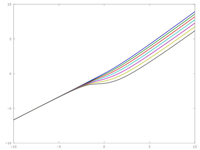
We start with the case of $\Lambda=0$, where we consider the possibility of having a non-vanishing background curvature $R_{b}$ determined via Eq. (49) from $S_{b}$; note that negative $S_{b}$ corresponds to positive curvature and vice versa. Fig. 1 shows a plot of ln($a_{\cal D}$) over ln($t$) for $S_{b}=0/-1/-2/-3/-4/-5/-6$. The fact that $V_{\cal D}=a_{\cal D}^{3}\sim t^{2}$ for small $t$ manifests itself by each of the lines starting with a slope of 2/3; an EdS universe would correspond to the case where the same linear relationship between ln($a_{\cal D}$) and ln($t$) would hold everywhere. Here and elsewhere we have chosen the convention of normalizing $a_{\cal D}$ in such a way that $a_{\cal D}^{3}/t^{2}\to 1$ for $t\to 0$; hence in the plot the straight line corresponding to EdS would pass through the origin of the plot. The effect of inhomogeneity on the case with $S_{b}=0$ (the highest, blue line) is just to change the slope somewhat. For the cases of $S_{b}<0$ the impact of having inhomogeneities is much more pronounced: without them, these universes would recollapse, but in their presence the overall expansion is just reduced while the regions that start with positive curvature collapse, and picks up speed again once the collapse is over. Of course our methods also work for $S_{b}>0$ ($R_{b}<0$) but the resulting universes are not very interesting since they look more or less like open FLRW universes.

Figure 2: ln($V_{\cal D}/t^{2}$) over ln($t$) for $S_{b}=0/-1/-2/-3/-4/-5/-6$

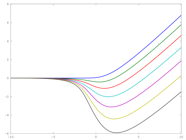
The next plot (Fig. 2), which diplays ln($a_{\cal D}^{3}/t^{2}$) over ln($t$), is just a linearly transformed version of the first one, which perhaps gives a better idea of how the inhomogeneities modify the evolution. Here the EdS case would correspond to a horizontal line. For the cases with nonzero background, one can clearly see the onset of collapse before the minority of expanding regions starts to control the overall behaviour.

Figure 3: $Ht$ over ln($t$) for $S_{b}=0/-1/-2/-3/-4/-5/-6$

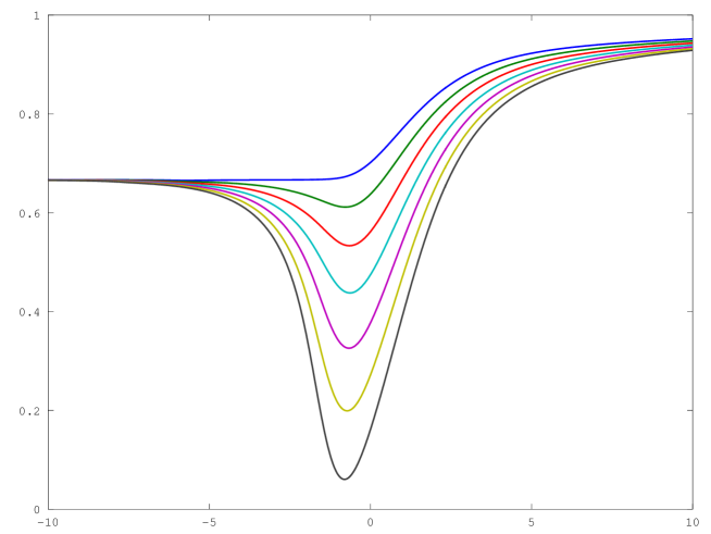
In Fig. 3 we see the graph of $Ht$ (with $H$ being, of course, $H_{\cal D}=\dot{a}_{\cal D}/a_{\cal D}$). Here we start again with the EdS value, which is $Ht=2/3$, and seem to converge very slowly towards the open FLRW case of $Ht=1$. The behaviour around $t\approx 1$ depends strongly upon the value of the background curvature: the higher $|S_{b}|$, the lower $Ht$ can go, and indeed for the case of $S_{b}=-7$ (not shown in the plot) we would get a phase of negative $\dot{a}_{\cal D}$, hence negative $Ht$.

Figure 4: Deceleration parameter over ln($t$) for $S_{b}=0/-1/-2/-3/-4/-5/-6$

Figure 5: Deceleration parameter over ln($t$) for $S_{b}=0/-1/-2/-3/-4$

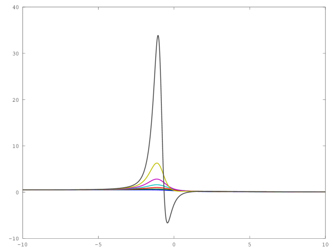
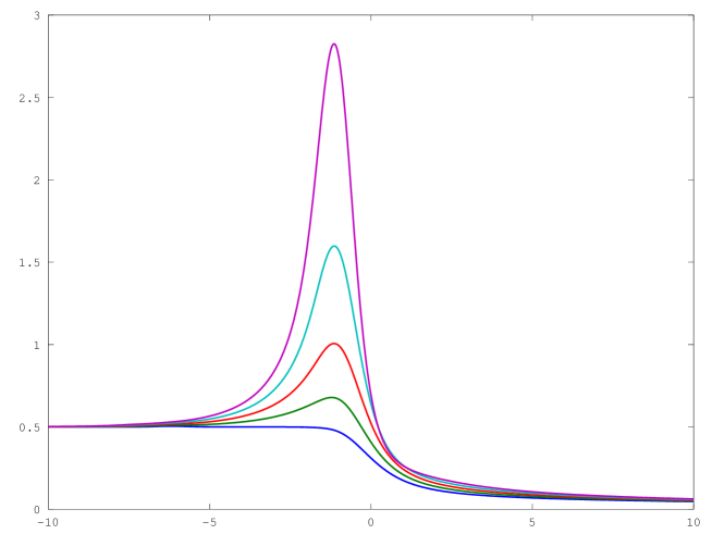
Fig. 4 and Fig. 5 display the deceleration parameter $q(t)=-\ddot{a}_{\cal D}a_{\cal D}/\dot{a}_{\cal D}^{2}$ over ln($t$). As Fig. 4 shows, the deceleration parameter can become significantly negative if the background curvature is large enough. In fact, $q$ diverges for higher values of $|S_{b}|$ since $\dot{a}_{\cal D}$ will then pass through zero. The asymptotic behaviour for $\ln(t)\to\pm\infty$ is easier to see in Fig. 5: again, near $t=0$ the EdS behaviour (with $q=1/2$) is approached, whereas for $t\to\infty$ a value of $q=0$ is approached, just like for an open universe.

Figure 6: Deceleration parameter over $Ht$ for $S_{b}=0/-1/-2/-3/-4/-5/-6$

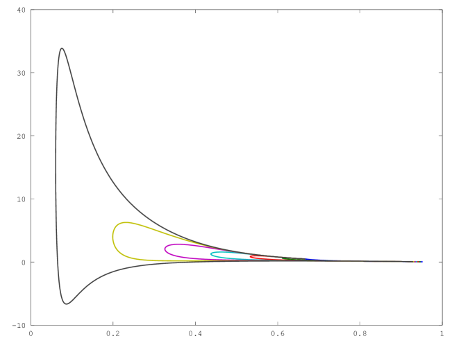
Fig. 6 combines data from the previous plots in a different way. Now the deceleration parameter $q$ is displayed over $Ht$.

Figure 7: Deceleration parameter over $Ht$ for $S_{b}=0/-1/-2/-3/-4/-5/-6$ (only $\ln(t)\geq 1/2$)

Fig. 7 shows the part of Fig. 6 that corresponds only to the values $\ln(t)\geq 1/2$, with a strongly expanded scale in the vertical direction corresponding to $q$. It is fairly clear from these plots that $Ht\approx 1$ and $q\approx-1/2$ cannot be achieved simultaneously by the present model with $\Lambda=0$.

4.2 Non-vanishing cosmological constant

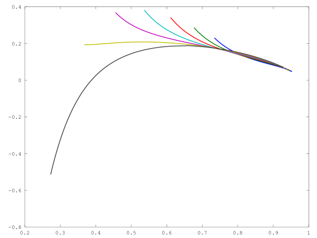
Let us now turn our attention to the case of $\Lambda>0$. In the following plots the curves correspond to values of $\Lambda$ with $\ln(\Lambda)\in\{+3,0,-3,-6,-9,-12,-15\}$ (remember that we are using the normalization conventions of Secs. 3.2, 3.3). Since current data seem to indicate that $Ht$ is very close to 1 presently, we are following the evolution of our universes only up to the point where $Ht$ exceeds $3/2$; this is the reason why the various curves seem to end prematurely.

Figure 8: ln($V_{\cal D}/t^{2}$) over ln($t$) for $\ln(\Lambda)=+3/0/-3/-6/-9/-12/-15$

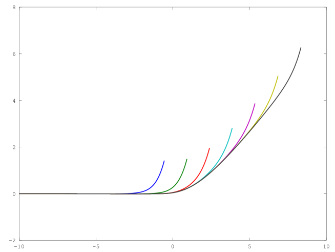
Fig. 8 shows again ln($V_{\cal D}/t^{2}$) plotted over ln($t$). There is no visible difference between the curves for $\ln(t)<-3$, and the whole graph looks like a single curve (which would, of course, just be the curve corrseponding to an inhomogeneous universe with $\Lambda=0$) sprouting arms at different locations. Let us briefly compare this with the standard FLRW case without inhomogeneities. In that case the same figure would look just like a straight line sprouting arms (we have checked that with our programs); similar statements hold for the next two figures.

Figure 9: $Ht$ over ln($t$) for $\ln(\Lambda)=+3/0/-3/-6/-9/-12/-15$

Figure 10: Deceleration parameter over ln($t$) for $\ln(\Lambda)=+3/0/-3/-6/-9/-12/-15$

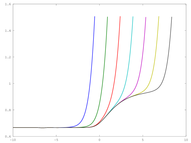
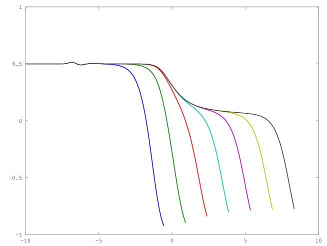
Figs. 9 and 10 again show $Ht$ and the deceleration parameter plotted over ln($t$) for our chosen values of $\Lambda$. The wiggle near $\ln(t)\approx-6$ is a numerical artefact that should be ignored.

Figure 11: Deceleration parameter over $Ht$ for $\ln(\Lambda)=+3/0/-3/-6/-9/-12/-15$

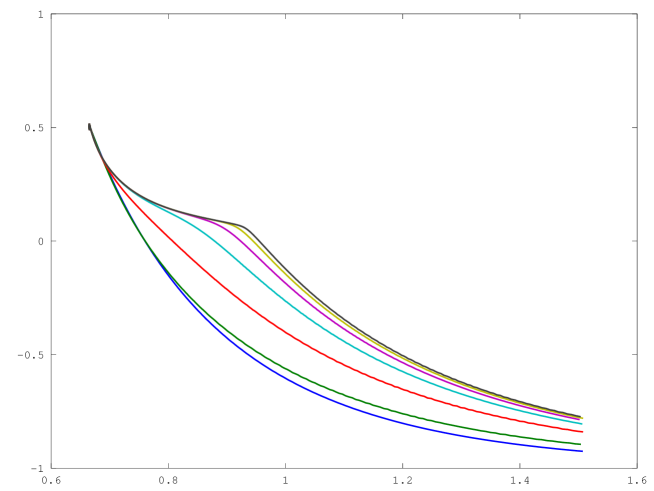
Fig. 11 is the analog of Fig. 6 for the case of $\Lambda\neq 0$, displaying again the deceleration parameter $q$ over $Ht$. In contradistinction to the case of $\Lambda=0$, it is now possible to produce the currently observed values for $Ht$ and $q$. This requires being close to the green (second lowest) curve which corresponds to a value of $\ln(\Lambda)=0$ in our dimensionless units. By taking another look at Figs. 9 and 10 we can identify the time when these values are taken (i.e., today) as corresponding to $\ln(t)\approx 0$ in our dimensionless units. We stress the fact that the occurrence of the values $\Lambda\approx 1$, $t\approx 1$ was not built into the model but emerged as a surprising result.

5 Discussion

Let us start the discussion of our results with the observation that we have an extremely predictive model: once values for the cosmological constant $\Lambda$ and the parameter $S_{b}$ controlling the background curvature have been chosen, the evolution of the volume of the universe is completely fixed. In order to compare the results of the model with observations, the only quantity that still needs to be determined is the scale of the time parameter. Inhomogeneity strongly affects the evolution of the universe, but it does not predict a negative deceleration parameter in a flat universe with $\Lambda=0$. If we assume that cosmological observations “see” the quantities $H_{\cal D}$ and $q_{\cal D}$ that we have computed (but see below for a brief discussion of this assumption), then Fig. 11 suggests that we should choose $\Lambda\approx 1$ and that the present age of the universe would correspond to $t\approx 1$. These statements refer to our dimensionless units where $t\approx 1$ is just the time when the inhomogeneities become relevant, and $\Lambda\approx 1$ is the value for which the effects of $\Lambda$ become strong precisely at that time. If this conclusion holds, it appears like yet another remarkable coincidence. Another possibility to calibrate our model would be to match it with the cosmic microwave background, where the deviations from uniformity that form the basis of our model have been measured to great precision. A comparison is not completely straightforward, however, since the quantity $\Delta_{\cal R}^{2}$ that parametrizes perturbations is usually quoted in terms of its Fourier modes, whereas in our approach we have integrated over them. For a comparison with $\Delta_{\cal R}^{2}$ we would have to evaluate the integral (59) completely, not just up to the constant $I$; unfortunately this integral would be infinite with the standard scale–invariant spectrum, so we would have to think carefully about the appropriate cutoff. Alternatively one could try to match the data directly to some of our formulas, such as Eq. (38). In order to assess the validity of our results, let us reiterate the simplifying assumptions that were made. The simplification that is most relevant to our model is the irrotational dust approximation. We know that this approximation breaks down both in the early universe and in regions that have virialized after contracting. As to the early universe, there certainly exist many observable effects (e.g. baryogenesis, baryon acoustic oscillations etc.) which cannot be explained within the irrotational dust setup. Clearly we should not apply our model to the era before matter domination. But matter domination starts approximately at the time of decoupling, when linear perturbation theory still provides an excellent description of the physics of the universe. Since our only assumptions on initial values are compatibility with linear perturbation theory and independence of the different Fourier modes, the breakdown of the irrotational dust approximation in the early universe should not lead to problems for our model. Regarding the treatment of collapsed regions, perhaps the simplest approach to estimating the effect of the ambiguity in modelling collapse is to directly compare different ways of treating collapsing regions. This can easily be done, with the result that this ambiguity seems to play a very minor role. For example, at $\Lambda=0$, $S_{b}=0$, $t=10$ we get $V_{\cal D}=126.62$ if we simply assume that there is no collapse at all, i.e. that any region that should collapse remains at its maximum volume; we get $V_{\cal D}=124.41$ if we assume that collapse is stopped at half the maximal extension (as we did for the results we presented in the previous section); and we get $V_{\cal D}=124.17$ if we allow such regions to collapse completely (i.e. to size zero). For smaller $t$ the differences are even smaller.

Figure 12: $a_{\cal D}$ plotted over $t$ for an EdS universe and versions 1.-3. of our model as presented in Sec. 3.2, with $\Lambda=0$ and $S_{b}=0$

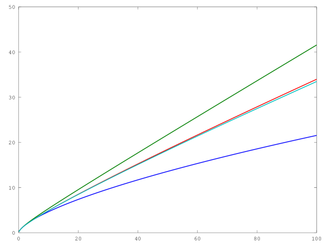
Another, possibly important source of imprecision is the treatment of the traceless part of the Ricci tensor. We discussed various possibilities in Sec. 3.2 around Eq. (55). While we cannot simulate the exact behaviour including what we called the $Y$-terms, we have performed the computations for the cases 1.-3. and compared them with the homogeneous EdS case. Fig. 12 displays the results, with each of the lines corresponding to a plot of $a_{\cal D}$ over $t$ for $\Lambda=0$ and $S_{b}=0$, for one of the following scenarios. The lowest (blue) line corresponds to an EdS universe. The highest (green) line corresponds to our first scenario, i.e. it takes into account the inhomogeneities, but ignores the impact of shear and the traceless part of the Ricci tensor as quantified by the last term in Eq. (28). The second highest (red) line indicates the result of scenario 2., where the inhomogeneous part $\bar{r}$ of the rescaled Ricci-tensor is modelled as constant. The line immediately below (shown in cyan) indicates scenario 3., i.e. the result of computing the evolution of $\bar{r}$ via Eq. (55). Note that all the lines would be much closer if we had chosen logarithmic scales as in the previous section. While it is obviously important to include the inhomogeneities and a nonzero value of $\bar{r}$, it does not seem to make much difference whether we take that quantity to be constant or whether we take into account those aspects of its evolution that are captured by Eq. (55). Therefore one would hope that the omission of the $Y$-terms should play a similarly small role; nevertheless, this is perhaps the weakest point of the present model. A minor source of uncertainty lies in our application of the results of Ref. [13]. Our assumption that only the function $C(x)$ is relevant relies on ignoring tensor modes and decaying modes. It is very hard to see how this might affect our results in a serious manner. Given the computational nature of the present results, one should also take into account the possibility of mistakes in programming and the effects of numerical imprecisions. It seems unlikely that such effects should modify the general conclusions of this work, for the following reason. During the programming phase, several mistakes were made and later eliminated, and in each case there was a change in numerical details of the results, but not in the overall structures. Therefore, even if there are still some factors of 2 or $\pi$ wrong in the programs, we would not expect a significant modification of the general conclusions. So, have we shown that a cosmological constant or dark energy is indeed needed to account for the results of observations? There may still be one important loophole: in our attempts to match the results of our computations with data, we have assumed that the various observational devices actually “see” the quantities $H_{\cal D}$ and $q_{\cal D}$ that we defined by volume averages in our inhomogeneous model universes. But there is no such thing as a device that can measure cosmological volumes directly. Instead, all the data come from photons that have travelled to us through an inhomogeneous universe. If light propagation in such a case is essentially equivalent to light propagation in a homogeneous universe with the scale factor $a_{\cal D}$, then there seems to be no escape from having to assume $\Lambda>0$; otherwise it would be possible that acceleration is simulated without taking place. In either case the methods presented here should provide useful tools for interpreting the results of precision cosmology. Acknowledgements: It is a pleasure to thank Anton Rebhan and Dominik Schwarz for helpful discussions.

Appendix: Details of the computation

The actual computations were performed numerically with the help of GNU octave [16]. The (integro-)differential equations (52) to (55) were discretized explicitly, using the Euler method. Two different approaches were implemented: on the one hand, equal steps $\epsilon=\bar{t}_{n+1}-\bar{t}_{n}$ were used to model the time parameter $\bar{t}$ itself; on the other hand $\ln\bar{t}$ was subjected to an equidistant discretization, resulting in a constant value for $\bar{t}_{n+1}/\bar{t}_{n}$. While the first (equal $\bar{t}$-steps) approach is more straightforward it is not so successful in combination with the $\bar{S}$– and $\bar{\delta}$–integrations in parameter space, where the finiteness of the range of $\bar{t}$ values quickly leads to problems. Here the second (equal ln–steps) approach, where even a moderate number of values $\bar{t}_{n}$ can span a reasonable range of orders of magnitude, is much more useful. Therefore only the second approach was applied to the cases with $\Lambda\neq 0$ or $S_{b}\neq 0$, and all of the figures shown in Sec. 4 were produced in this way. However, the equal $\bar{t}$-steps approach was used for comparing different ways of modelling collapse and for studying the impact of various assumptions on the traceless part of the Ricci tensor (Fig. 12). For $\Lambda=0$, $S_{b}=0$ the results from both routines were compared and found to agree up to differences that would be expected as errors coming from the discretization. These two approaches were implemented in the following ways.

Equal $\bar{t}$-steps

With this approach only the case of $\Lambda=0$, $S_{b}=0$ was studied. We found it useful to choose

$$q=\sqrt{{\bar{S}^{2}\over 5}+\bar{\delta}^{2}},\quad\bar{S}=\sqrt{5}\,q\cos\vartheta,\quad\bar{\delta}=q\sin\vartheta,$$ (70)

so that Eq. (69) becomes

$$V_{\cal D}(\bar{t}) \sim \int\bar{a}^{3}(\bar{t};\sqrt{5}\,q\cos\vartheta,q\sin\vartheta,\varphi)e^{-{q^{2}\over 2}}q^{5}\,\sin^{4}\vartheta\,\sin(3\varphi)dq\,d\vartheta d\varphi$$ (71)

$$\sim \int\bar{a}^{3}(q^{3\over 2}\bar{t};\sqrt{5}\,\cos\vartheta,\sin\vartheta,\varphi)e^{-{q^{2}\over 2}}q^{2}\,\sin^{4}\vartheta\,\sin(3\varphi)dq\,d\vartheta d\varphi$$ (72)

$$\sim {1\over\bar{t}^{2}}\int\bar{a}^{3}(\bar{t}^{\prime};\sqrt{5}\,\cos\vartheta,\sin\vartheta,\varphi)e^{-{1\over 2}({{\bar{t}^{\prime}}\over{\bar{t}}})^{4\over 3}}{\bar{t}^{\prime}}\,\sin^{4}\vartheta\,\sin(3\varphi)d{\bar{t}^{\prime}}\,d\vartheta d\varphi,$$ (73)

where we first used Eq. (56) and then performed a change of variables from $q$ to ${\bar{t}^{\prime}}=q^{3\over 2}\bar{t}$. In evaluating the last expression numerically, we started with the $\varphi$–integration (whenever it was applied; see below), proceeded with the $\vartheta$–integration and finally performed the $\bar{t}^{\prime}$–integration. By keeping only the results of the integrations, the required memory could be kept very small. While the first two integrations worked well, the last one showed good convergence properties only for a limited range of $\bar{t}$–values. This approach was used to compare the different scenarios for modelling $\bar{r}$ as presented in the paragraph around Eq. (55), with the result that, while there are great differences between a homogeneous universe and the universes corresponding to the scenarios 1. and 2., the difference between the scenarios 2. and 3. (the latter being the only one requiring the $\varphi$–integration) were quite small.

Equal steps for ln($\bar{t}$)

The complete range $(0,\infty)$ for $\bar{t}$ was divided into three parts. While the solution was performed numerically in the middle part, an approximation by linear perturbation theory was used for $\bar{t}<\!\!<1$ and an approximation by a closed formula for $\bar{t}\in[\bar{t}_{\mathrm{final}},\infty)$. The choice of formula depended on the context: for collapsing solutions, $\bar{t}_{\mathrm{final}}$ was the time step at which the solution for $\bar{a}$ would have dropped below half of the maximum value $\bar{a}_{\mathrm{max}}$, and $\bar{a}(\bar{t})$ was taken to be $\bar{a}_{\mathrm{max}}/2$ for $\bar{t}\geq\bar{t}_{\mathrm{final}}$; in the non-collapsing case $\bar{a}^{3}$ was modelled as the de Sitter solution $\mathrm{const}\times\exp(\sqrt{3\Lambda}\,t)$ for $\Lambda>0$, and as a cubic function of $\bar{t}$ otherwise, with $\bar{t}_{\mathrm{final}}$ chosen in such a way that these approximations were sufficiently good. Since the results of the equal $\bar{t}$-steps approach indicated that the contribution of the term (55) was not significant, it was omitted here, resulting in the simplification that no $\varphi$–integration was required. While we did not consider the case with both $\Lambda$ and $S_{b}$ non-vanishing, we did study the following two scenarios.

• Flat background with a cosmological constant:
  Parametrizing $\bar{S}$ and $\bar{\delta}$ as in (70) we find

  $$V_{\cal D}(\bar{t};\bar{\Lambda}) \sim \int\bar{a}^{3}(\bar{t};\sqrt{5}\,q\cos\vartheta,q\sin\vartheta,\bar{\Lambda})e^{-{q^{2}\over 2}}q^{5}\,\sin^{4}\vartheta\,dq\,d\vartheta$$ (74)

  $$\sim \int\bar{a}^{3}(q^{3\over 2}\bar{t};\sqrt{5}\,\cos\vartheta,\sin\vartheta,q^{-3}\bar{\Lambda})e^{-{q^{2}\over 2}}q^{2}\,\sin^{4}\vartheta\,dq\,d\vartheta.$$ (75)

  Again it is useful to perform the $\vartheta$–integration first. In this way we generated a list of $\vartheta$–integrated solutions for different values of $\bar{\Lambda}$, with steps in ln($\bar{\Lambda}$) twice the size of the ln($\bar{t}$)–steps. Then computing $V_{\cal D}(\bar{t};\bar{\Lambda})$ numerically according to Eq. (75) corresponded to just one “diagonal” (rising $\bar{t}$, falling $\bar{\Lambda}$) summation over this list.

• Curved background without a cosmological constant:
  Now taking $q=\bar{\delta}$ in Eq. (56) we arrive at

  $$V_{\cal D}(\bar{t};\bar{S}_{b}) \sim \int\bar{a}^{3}({\bar{t}};\bar{S},\bar{\delta})e^{-{1\over 10}(\bar{S}-\bar{S}_{b})^{2}-{1\over 2}\bar{\delta}^{2}}\bar{\delta}^{4}\,d\bar{S}\,d\bar{\delta}$$ (76)

  $$\sim \int\bar{a}^{3}(\bar{\delta}^{3\over 2}{\bar{t}};{\bar{S}\over\bar{\delta}},1)e^{-{1\over 10}(\bar{S}-\bar{S}_{b})^{2}-{1\over 2}\bar{\delta}^{2}}\bar{\delta}\,d\bar{S}\,d\bar{\delta}.$$ (77)

  This was evaluated by first generating a list of solutions $\bar{a}(\bar{t},\bar{S},1,0)$, then performing the $\bar{\delta}$–integration of Eq. (77) which resulted in another list indexed by different $\bar{S}$–values, and finally integrating over $\bar{S}$.

The numerical parameters (step widths, values at which the description changes from perturbation theory to explicit computation, etc.) were chosen pragmatically in such a way that a further refinement would not lead to clearly discernible effects in the plots; an exception is the wiggle in Fig. 9 which could have been reduced only by a very time consuming increase in the number of steps. For producing the plots of Sec. 4 we took the stepwidth in ln($t$) to be $2^{-7}$, divided the interval $[0,\pi]$ for $\vartheta$ into $2^{8}$ parts, created a list of solutions for values $\ln(\Lambda)\in[-27,9]$ (with a stepwidth of $2^{-6}$, i.e. twice the value of that for $\ln(t)$), and similarly chose further parameters. The differentiations required to compute $H$ and $q$ were performed numerically with formulas such as

$$H(t_{n})\,t_{n}={d\ln(a)\over d\ln(t)}(t_{n})\approx{\ln(a_{n+1})-\ln(a_{n-1})\over\ln(t_{n+1})-\ln(t_{n-1})}.$$ (78)

This worked quite well in general. The exceptions were the aforementioned wiggle, as well as a spike that would have occurred in Figs. 4 and 5 as a consquence of the transition between different regimes; its artificiality was clear from the fact that it became larger when the stepwidth was refined. For producing the figures we simply removed the two offending data points by hand.