Cell-Probe Bounds for Online Edit Distance and
Other Pattern Matching Problems

Abstract

We give cell-probe bounds for the computation of edit distance, Hamming distance, convolution and longest common subsequence in a stream. In this model, a fixed string of $n$ symbols is given and one $\delta$-bit symbol arrives at a time in a stream. After each symbol arrives, the distance between the fixed string and a suffix of most recent symbols of the stream is reported. The cell-probe model is perhaps the strongest model of computation for showing data structure lower bounds, subsuming in particular the popular word-RAM model.

• We first give an $\Omega\big{(}(\delta\log n)/(w+\log\log n)\big{)}$ lower bound for the time to give each output for both online Hamming distance and convolution, where $w$ is the word size. This bound relies on a new encoding scheme and for the first time holds even when $w$ is as small as a single bit.

• We then consider the online edit distance and longest common subsequence problems in the bit-probe model ($w=1$) with a constant sized input alphabet. We give a lower bound of $\Omega(\sqrt{\log{n}}/(\log{\log{n}})^{3/2})$ which applies for both problems. This second set of results relies both on our new encoding scheme as well as a carefully constructed hard distribution.

• Finally, for the online edit distance problem we show that there is an $O((\log^{2}{n})/w)$ upper bound in the cell-probe model. This bound gives a contrast to our new lower bound and also establishes an exponential gap between the known cell-probe and RAM model complexities.

1 Introduction

The search for lower bounds in general random-access models of computation provides some of the most important and challenging problems within computer science. In the offline setting where all the data representing the problem are given at once, non-trivial, unconditional, time lower bounds still appear beyond our reach. One area where there has however been success in proving time lower bounds is in the field of dynamic data structure problems (see for example [8, 17, 15, 12, 11] and references therein) and online or streaming problems [3, 4].

We consider streaming problems where there is a given fixed array of $n$ values and a separate stream of values that arrive one at a time. After each value arrives in the stream, a function of the fixed array and the latest values of the stream is computed and reported. We consider several fundamental measures: edit distance, Hamming distance, inner product/convolution and longest common subsequence (LCS). Efficiently finding patterns in massive and streaming data is a topic of considerable interest because of its wide range of practical applications.

For each problem we give new cell-probe lower bounds. For the edit distance problem we also provide a cell-probe upper bound that is exponentially faster than was previously known. The cell-probe model is perhaps the strongest model of computation for showing data structure lower bounds, subsuming in particular the popular word-RAM model.

Hamming distance and convolution

Our first set of results concern cell-probe lower bounds for Hamming distance and convolution. For brevity, we write $[q]$ to denote the set $\{0,\dots,q-1\}$, where $q$ is a positive integer.

Problem 1 (Online Hamming distance and convolution).

For a fixed array $F\in[q]^{n}$ of length $n$, we consider a stream in which symbols from $[q]$ arrive one at a time. In the online Hamming distance problem, for each arriving symbol, before the next value arrives, we output the Hamming distance between $F$ and the array consisting of the latest $n$ values of the stream. In the convolution problem, the output is instead the inner product between $F$ and the latest $n$ values in the stream.

We show a lower bound for the expected amortised time per output of any randomised algorithm that solves either the Hamming distance or convolution problem. Throughout the paper we let $w$ denote the word size and $\delta=\lfloor\log_{2}{q}\rfloor$.

Theorem 1.

In the cell-probe model with any word size $w$ and positive integer $q$, the expected amortised time per output of any randomised algorithm that solves either the Hamming distance problem or the convolution problem is

$$\Omega{\left(\frac{\delta\log n}{w+\log\log n}\right)}.$$

This lower bound also holds even when outputs are reported modulo $q$.

These lower bounds can be compared with the known $O((\delta/w)\log{n})$ time upper bounds for both the online Hamming distance and convolution in the cell-probe model [2, 4]. To obtain these results we first provide a new method that gives a straightforward and clean unifying framework for streaming lower bounds in the cell-probe model with small word sizes. This itself marks a methodological advance in the development of lower bounds for streaming problems.

Cell-probe lower bounds of $\Omega((\delta/w)\log{n})$ time per output for the convolution problem [3] and Hamming distance problem [4] had previously been shown only when the word size $w\in\Omega(\log{n})$. These bounds were therefore meaningful only when $\delta$, the number of bits needed to represent a symbol, was sufficiently large, typically $\Theta(\log{n})$. From a practical point of view it is arguable that such very large input alphabets are rarely seen. Our improved lower bound gives a smooth trade-off that holds for word and symbol sizes as small as a single bit. In the perhaps most interesting case where $\delta=w$ we therefore show an $\Omega(\log{n})$ lower bound for $w\in\Omega(\log{\log{n}})$. In the bit-probe model (i.e. $w=1$), our results imply an $\Omega(\log^{2}{n}/\log{\log{n}})$ lower bound when $\delta=\Omega(\log{n})$. We are also able to obtain interesting lower bounds for smaller values of $\delta$, in particular an $\Omega(\log{n}/\log{\log{n}})$ lower bound for binary inputs ($\delta=1$) in the bit-probe model. The bit-probe model is considered theoretically appealing due to its machine independence and overall cleanliness [13, 16].

In the unit-cost word-RAM model with $w,\delta\in\Theta(\log n)$, the Hamming distance problem can be solved in $O(\sqrt{n\log{n}})$ time per arriving symbol, and the convolution problem can be solved in $O(\log^{2}n)$ time per arriving symbol [2]. The lower bounds we give therefore might appear distant from the known RAM model upper bounds in the case of Hamming distance. However, an online-to-offline reduction of [2] also tells us that any improvement to the online lower bound in the RAM model would imply a new super-linear and offline RAM model lower bound. As no such lower bound is known for any problem in NP this seems a not inconsiderable barrier.

Edit distance and LCS

Our next set of results concern edit distance and longest common subsequence (LCS), for which no previous, non-trivial cell-probe bounds were known. For the edit distance and LCS problems we define $S(k)$ to be the $k$-length string representing the most recent $k$ symbols in the stream and $\textup{Edit}(A,B)$ to be the minimal number of single symbol edit operations (replace, delete and insert) required to transform string $A$ into string $B$. Analogously, $\textup{LCS}(A,B)$ is defined to be the length of an LCS of $A$ and $B$.

In our online setting, the natural way of defining edit distance is by minimising the distance over all suffixes of the stream. For the related LCS problem we take a slightly different approach to avoid the LCS rapidly converging to the entire fixed string $F$. As a result we consider a fixed length sliding window of the stream instead, as in the Hamming distance problem.

Problem 2 (Online edit distance and LCS).

For a fixed string $F\in[q]^{n}$ of length $n$, we consider a stream in which symbols from $[q]$ arrive one at a time. In the edit distance problem, for each arriving symbol we output $\min_{k}\textup{Edit}(F,S(k))$. In the longest common subsequence (LCS) problem, for each arriving symbol we output $\textup{LCS}(F,S(n))$.

We show a lower bound for the expected amortised time per output of any randomised algorithm that solves either the edit distance problem or the LCS problem.

Theorem 2.

In the cell-probe model, where the word size $w=1$ and the alphabet size is at least 4, the expected amortised time per output of any randomised algorithm that solves either the edit distance problem or the LCS problem is

$$\Omega{\left(\frac{\sqrt{\log{n}}}{(\log{\log{n}})^{3/2}}\right)}.$$

This lower bound holds even when the outputs are succinctly encoded.

A property of both these problems is that any two consecutive outputs differ by at most one. This allows each output to be specified in a constant number of bits. The restriction on the word and input alphabet size in Theorem 2 derives directly from the ability to encode the output succinctly and its necessity will become clearer when we describe the proof technique.

It is at first tempting to believe that there may be a simple reduction between the edit distance, LCS and Hamming distance problems which will allow us to derive lower bounds without requiring further work. Although such direct reductions appear elusive in our streaming setting, we are able to exploit more subtle and indirect relationships between the distance measures to obtain our lower bounds.

We complement our edit distance lower bound with a new cell-probe algorithm which runs in polylogarithmic time per arriving symbol.

Theorem 3.

In the cell-probe model with any word size $w$ and alphabet size that is polynomial in $n$, the edit distance problem can be solved in

$$O{\left(\frac{\log^{2}n}{w}\right)}$$

amortised time per output.

The fastest RAM algorithm for online edit distance runs in $O(n)$ time by simply adding a new column to the classic dynamic programming matrix for each new arrival. Despite the computation of edit distance being a widely studied topic, it is not at all clear how one can do significantly better than this naive approach given the dependencies which seem to be inherent in the standard dynamic programming formulation of the problem. We believe it is therefore of independent interest for those studying the edit distance that there is now an exponential gap between the known RAM and cell-probe complexities. It is still unresolved whether a similarly fast cell-probe algorithm exists for the online LCS problem.

1.1 Prior work

The field of streaming algorithms is well studied and the specific question of how efficiently to find patterns in a stream is a fundamental problem that has received increasing attention over the past few years. In a classic result of Galil’s [9] from the early 1980s, exact matching was shown to be solvable in constant time per arriving symbol in a stream. Nearly 30 years later a general online-to-offline reduction was shown which enables many offline algorithms to be made online with a worst case logarithmic factor overhead in the time complexity per arriving symbol in the stream [1]. For some problems, this reduction gives us the best time complexity known, but in other cases it is possible to do even better. One example where a more efficient online algorithm exists is the $k$-mismatch problem, which has an $O(n\sqrt{k\log k})$ complexity offline but $O(\sqrt{k}\log{k}+\log{m})$ time per new arriving symbol online [6], where $n$ is the length of the text and $m$ is the length of the pattern.

The online-to-offline reduction of [1] does not however lend itself to problems that can be described as non-local. The distance function between two strings of the same length is said to be local if it is the sum of the disjoint contribution from each aligned pair of symbols. For example, Hamming distance is a local distance function whereas edit distance is non-local. Streaming pattern matching upper bounds have also been developed for a range of non-local problems, including function matching, parameterised matching, swap distance, $k$-differences as well as others [5]. These algorithms have necessarily been particular to each distance function.

Given the rarity of constant time streaming algorithms, it is therefore natural to ask for lower bounds; what are the limits of how fast a streaming pattern matching problem can be solved? The first steps towards an answer to this question were given in [3], where a lower bound for convolution, or equivalently the cross-correlation, was given. Computing cross-correlations is an important component of many of the fastest pattern matching algorithms. By giving a lower bound for the time to perform the cross-correlation, a lower bound is therefore provided for a whole class of pattern matching algorithms. However the question of whether a particular pattern matching problem could be solved by some other faster means remained open. In [4], the three authors of this paper gave the first lower bound for a pattern matching problem. The streaming Hamming distance problem was shown to have a logarithmic lower bound when the input alphabet size is sufficiently large. This provided the first separation between two pattern matching problems: exact matching, which can be solved in constant time, and Hamming distance which cannot.

1.2 The cell-probe model

Our bounds hold in the cell-probe model which is a particularly strong model of computation, introduced originally by Minsky and Papert [14] in a different context and then subsequently by Fredman [7] and Yao [19]. The generality of the cell-probe model makes it attractive for establishing lower bounds for dynamic data structure problems, and many such results have been given in the past couple of decades. The approaches taken had historically been based only on communication complexity arguments and the chronogram technique of Fredman and Saks [8], which until recently were able to prove $\Omega(\log{n}/\log{\log{n}})$ lower bounds at best. There remains however, a number of unsatisfying gaps between the lower bounds and known upper bounds. However, in 2004, a breakthrough led by Pǎtraşcu and Demaine gave us the tools to seal the gaps for several data structure problems [17] as well as giving the first $\Omega(\log{n})$ lower bounds. This new technique is based on information theoretic arguments that we also employ here.

In the cell-probe model there is a separation between the computing unit and the memory, which is external and consists of an (unbounded) array of cells of $w$ bits each. The computing unit has no internal memory cells of its own. Any computation performed is free and may be non-uniform. The cost of processing an update or query (in our case outputting the answer when a value in the stream arrives) is the number of distinct cells accessed (cell-probes) during that update, or query. This general view makes the model very strong. In particular, any lower bounds in the cell-probe model hold in the word-RAM model (with the same cell size). In the word-RAM model, certain operations on words, such as addition, subtraction and possibly multiplication, take constant time (see for example [10] for a detailed introduction). Although in our case we place no minimum size restriction on the size of a word, much of the previous work has required that words are sufficiently large to be able to store the address of any cell of memory. When the word size $w=1$ then our new lower bounds also hold, for example, for the weaker multi-head Turing machine model with a constant number of heads.

1.3 Technical contributions

New lower bounds

One of the most important techniques for online lower bounds is based on the information transfer method of Pǎtraşcu and Demaine [17]. For a pair of time intervals, the information transfer is the set of memory cells that are written during the first interval, read in the next and not overwritten in between. These cells must contain all the information from the updates during the first interval that the algorithm needs in order to produce correct outputs in the next interval. If one can prove that this quantity is large for many pairs of intervals then the desired lower bounds follow. To do this we relate the size of the information transfer to the conditional entropy of the outputs in the relevant time interval. The main task of proving lower bounds reduces to that of devising a hard input distribution for which outputs have high entropy conditioned on selected previous values of the input.

Previous applications of the information transfer technique have required that the word size $w$ is $\Omega(\log n)$ [17, 2, 4]. To circumvent this limitation we have developed a new encoding of the information transfer that is efficient for arbitrarily small values of $w$, in particular $w=1$ as in the bit-probe model. The overall method is to combine an encoding based on cell addresses with a new encoding that identifies a cell with the time step at which it is read. This combination of two encodings enables us to prove new lower bounds for the convolution and Hamming distance problems. Moreover it is a crucial first step in developing our new lower bounds for the edit distance and LCS problems where we restrict our attention to constant sized alphabets.

The edit distance and LCS problems raise a number of challenges not presented by either of the other two problems we consider. These distance measures are what we call non-local. Focusing on the LCS problem for the moment we can see that whether position $i$ of the fixed array is included in the LCS or not depends not only on the value in the stream that is aligned with $i$ but also on other values in the stream. The information transfer technique has previously not been applied to such non-local streaming problems. The main technical difficulty that non-local distance measures introduce is a blurring of the borders between intervals.

We describe a hard input distribution of the LCS problem for which the information transfer technique is indeed applicable. The idea is to construct a fixed array and a random input stream such that at many alignments, from the length of the LCS one can obtain the Hamming distance between the fixed array and the corresponding portion of the stream. In order to then apply the information transfer technique we must prove that this direct relationship between the length of the LCS and Hamming distance occurs with sufficiently large probability. This is one of the more technical parts of the paper. Once we have obtained a lower bound for the LCS problem we show that the same lower bound holds also for the edit distance problem. This follows from our LCS hard distribution combined with a squeezing lemma that forces the edit distance to equal the Hamming distance at certain alignments.

New upper bound

Our cell-probe algorithm for edit distance is a non-trivial modification of the classic dynamic programming solution which allows us to take advantage of the fact that computation is free in the cell-probe model. We exploit the relationship between edit distance and shortest paths in a directed acyclic graph (DAG). The nodes in the graph form a lattice and the current edit distance is the shortest path from the top-left node to the bottom-right node. Each new symbol that arrives simply adds a new column of distances. This update operation is however slow even in the cell-probe model; just writing the new values to memory requires $\Theta(n/w)$ cell probes. Our algorithm circumvents this problem.

The first key difference between our new method and the naive approach is that instead of maintaining only the values of the latest column, we maintain values from the $n$ latest columns. We maintain values denoted $D(j,i)$, where $D(j,i)$ is the shortest path from the top-left to the node $(j,i)$ in the DAG over paths that are forced to go via selected previous nodes. Further, we do not in fact maintain $D(j,i)$ for all rows $j$, potentially leaving gaps in the table. As a result we can efficiently maintain the $D(j,i)$ values. Despite the fact that our algorithm does not correctly compute the whole dynamic programming table we are able to show that for all $i$, the outputted value $D(n-1,i)$ still is the correct edit distance after symbol $S[i]$ has arrived.

1.4 Organisation

In Section 2 we set up some basic notation and give problem definitions. In Section 3 we describe how to obtain the lower bounds. This section contains some key lemmas which are solved separately in subsequent sections. In Section 4 we describe the hard distribution for the edit distance and the LCS problems. In Section 6 we explain the new encoding scheme that we use with the information transfer method. Finally, in Section 7 we give the cell-probe algorithm that solves the edit distance problem. This section can be read in isolation and does not build on previous sections.

2 Basic setup for the lower bounds

In this section we introduce notation and concepts that are used heavily in the lower bound proofs. We also formally define the streaming problems in our new notation.

2.1 Basic notation

For a positive integer $n$, $[n]$ denotes the set $\{0,\dots,n-1\}$. For an array $A$ of length $n$ and $i,j\in[n]$, we write $A[i]$ to denote the value at position $i$, and where $j\geqslant i$, $A[i,j]$ denotes the $(j-i+1)$-length subarray of $A$ starting at position $i$. All logarithms are in base two and we assume that $n\geqslant 4$ throughout.

We define a streaming problem as follows. There is a fixed array $F$ of length $n$ and an array $S$ of length $3n$, which is referred to as the stream. Both $F$ and $S$ are over the set $[2^{\delta}]$ of integers, referred to as the alphabet, where $\delta$ is a positive integer and is a parameter of the problem. An element of the alphabet is often referred to as a symbol. We let $t\in[n]$ denote the arrival time, or simply arrival of the symbol $S[2n+t]$. That is, for $t=0$, just before the symbol $S[2n]$ arrives, the stream already contains $2n$ symbols. To capture the concept of a data stream, not all symbols of $S$ are immediately available. More precisely, just after arrival $t\in[n]$ only the symbols of $S[0,2n+t]$ are known, and importantly, the symbols $S[(2n+t+1),(3n-1)]$ are not known. That is one new symbol is revealed at a time. We define

$$S_{t}=S[(n+1+t),(2n+t)]$$

to denote latest $n$ symbols of the stream up to arrival $t$. Once the symbol at arrival $t$ is revealed, and before the next symbol at arrival $t+1$ is revealed, a function of $F$ and $S[0,2n+t]$ is computed and its value outputted. We let the $n$-length array $Y$ denote the outputs such that $Y[t]$ is outputted immediately after arrival $t$. The outputs depend on which streaming problem is considered:

• In the Hamming distance problem, $Y[t]=\textup{Ham}(F,S_{t})$, which is number of positions $i\in[n]$ such that $F[i]\neq S_{t}[i]$.

• In the convolution problem, $Y[t]=\sum_{i\in[n]}F[i]\cdot S_{t}[i]$.

• In the edit distance problem, $Y[t]=\min_{i\in[2n+1+t]}\textup{Edit}(F,S[i,2n+t])$.

• In the longest common subsequence (LCS) problem, $Y[t]=\textup{LCS}(F,S_{t})$, which is the length of the LCS of $F$ and $S_{t}$.

2.2 Information transfer and more notation

Our lower bounds hold for any randomised algorithm on its worst case input. The approach to obtain such bounds is by applying Yao’s minimax principle [18]. That is, we show that the lower bounds of Theorems 1 and 2 hold for any deterministic algorithm on some random input. This means that we will devise a fixed array $F$ and describe a probability distribution for the stream $S$. We then show a lower bound on the expected running time over $n$ symbol arrivals in the stream that holds for any deterministic algorithm. Due to the minimax principle, the same lower bound must then hold for any randomised algorithm on its worst case input. The amortised bound is obtain by dividing by $n$. From this point onwards, we consider an arbitrary deterministic algorithm running with some fixed array $F$ on a random stream $S$. As it is used to show a lower bound, such an $F$ and distribution on $S$ is referred to as a hard distribution.

The information transfer tree, denoted $\mathcal{T}$, is a balanced binary tree over $n$ leaves. To avoid technicalities we assume that $n$ is a power of two. For a node $v$ of $\mathcal{T}$, we let $\ell_{v}$ denote the number of leaves in the subtree rooted at $v$. The leaves of $\mathcal{T}$, from left to right, represent the arrival $t$ from $0$ to $n-1$. An internal node $v$ is associated with three arrivals, $t_{0}$, $t_{1}$ and $t_{2}$. Here $t_{0}$ is the arrival represented by the leftmost node in subtree rooted at $v$, similarly $t_{2}=t_{0}+\ell_{v}-1$ is the rightmost such node and $t_{1}=t_{0}+\ell_{v}/2-1$ is in the middle. That is, the intervals $[t_{0},t_{1}]$ and $[t_{1}+1,t_{2}]$ span the left and right subtrees of $v$, respectively. We define the subarray $\mathcal{S}_{v}=S[2n+t_{0},2n+t_{1}]$ to represent the $\ell_{v}/2$ stream symbols arriving during the arrival interval $[t_{0},t_{1}]$, and we define the subarray $Y_{v}=Y[t_{1}+1,t_{2}]$ to represent the $\ell_{v}/2$ outputs during the arrival interval $[t_{1}+1,t_{2}]$. We define $\widetilde{\mathcal{S}}_{v}$ to be the concatenation of $S[0,(2n+t_{0}-1)]$ and $S[(2n+t_{1}+1),(3n-1)]$. That is, $\widetilde{\mathcal{S}}_{v}$ contains all symbols of $S$ except for those in $\mathcal{S}_{v}$.

When $\widetilde{\mathcal{S}}_{v}$ is fixed to some constant $\widetilde{s}_{v}$ and $\mathcal{S}_{v}$ is random, we write $H(Y_{v}\mid\widetilde{\mathcal{S}}_{v}=\widetilde{s}_{v})$ to denote the conditional entropy of $Y_{v}$ under the fixed $\widetilde{\mathcal{S}}_{v}$.

We define the information transfer of a node $v$ of $\mathcal{T}$, denoted $\mathcal{I}_{v}$, to be the set of memory cells $c$ such that $c$ is written during the interval $[t_{0},t_{1}]$, read at some time in $[t_{1}+1,t_{2}]$ and not overwritten in $[t_{1}+1,t_{2}]$ before being read for the first time in $[t_{1}+1,t_{2}]$. The cells in the information transfer $\mathcal{I}_{v}$ therefore contain, by definition, all the information about the values in $\mathcal{S}_{v}$ that the algorithm uses in order to correctly produce the outputs $Y_{v}$. By adding up the sizes of the information transfers $\mathcal{I}_{v}$ over all nodes $v$ of $\mathcal{T}$, we get a lower bound on the total running time (that is, the number of cell reads). To see this, it is important to make the observation that a cell read of $c\in\mathcal{I}_{v}$ at arrival $t$ will be accounted for only in the information transfer of node $v$ and not in the information transfer of a node $v^{\prime}\neq v$. As a shorthand for the size of the information transfer, we define $I_{v}=|\mathcal{I}_{v}|$. Our aim is to show that $I_{v}$ is large in expectation for a substantial proportion of the nodes $v$ of $\mathcal{T}$.

3 Overall proofs of the lower bounds

In this section we give the overall proofs for the main lower bound results of Theorems 1 and 2. Let $v$ be any node of $\mathcal{T}$. Suppose that $\widetilde{\mathcal{S}}_{v}$ is fixed but the symbols in $\mathcal{S}_{v}$ are randomly drawn in accordance with the distribution on $S$, conditioned on the fixed value of $\widetilde{\mathcal{S}}_{v}$. This induces a distribution on the outputs $Y_{v}$. If the entropy of $Y_{v}$ is large, conditioned on the fixed $\widetilde{\mathcal{S}}_{v}$, then any algorithm must probe many cells in order to produce the outputs $Y_{v}$, as it is only through the information transfer $\mathcal{I}_{v}$ that the algorithm can know anything about $\mathcal{S}_{v}$. We will soon make this claim more precise. We first define a high-entropy node in the information transfer tree.

Definition 1 (High-entropy node).

A node $v$ in $\mathcal{T}$ is a high-entropy node if there is a positive constant $k$ such that for any fixed $\widetilde{s}_{v}$,

$$H(Y_{v}\mid\widetilde{\mathcal{S}}_{v}=\widetilde{s}_{v})\,\geqslant\,k\cdot\delta\cdot\ell_{v}.$$

To put this bound in perspective, note that the maximum conditional entropy of $Y_{v}$ is bounded by the entropy of $\mathcal{S}_{v}$, which is at most $\delta\cdot(\ell_{v}/2)$ and obtained when the values of $\mathcal{S}_{v}$ are independent and uniformly drawn from $[2^{\delta}]$. Thus, the conditional entropy associated with a high-entropy node is the highest possible up to some constant factor. As we will see, this is good news for proving lower bounds, and for the Hamming distance and convolution problems we have many high-entropy nodes. The following fact tells us that there are inputs with many high-entropy nodes.

Lemma 1.

For both the Hamming distance and convolution problems, where outputs are given modulo $2^{\delta}$, there exists a hard distribution and a constant $c>0$ such that $v\in\mathcal{T}$ is a high-entropy node if $\ell_{v}\geqslant c\cdot\sqrt{n}$.

Proof.

For the convolution problem, the lemma is equivalent to Lemma 2 of Clifford and Jalsenius [3], although notations differ and here we only consider nodes $v$ such that $\ell_{v}\geqslant c\cdot\sqrt{n}$.

For the Hamming distance problem, the statement of the lemma is equivalent to Lemma 2.2 of Clifford, Jalsenius and Sach [4] with the only difference that in our lemma above we give outputs modulo $2^{\delta}$. In the previous work of [4], $2^{\delta}\in\Theta(n)$, but here we consider any arbitrary $\delta$. For this reason it is not obvious that Lemma 2.2 of [4] applies under the modulo constraint. However, by inspection of the details in [4], we see that every output is given within a range of size $2^{\delta}$, hence the lemma is indeed applicable also with the modulo constraint. ∎

For the edit distance and LCS problems on the other hand, the maximum conditional entropy of $Y_{v}$ is at most $O(\ell_{v})$, independent of $\delta$. This is because the outputs can be encoded succinctly. Therefore we cannot expect to obtain high-entropy nodes for these problems in general. Moreover, it is not even clear whether high-entropy nodes can be obtained for constant $\delta$. For these two problems we therefore rely on what we call medium-entropy nodes.

Definition 2 (Medium-entropy node).

A node $v$ in $\mathcal{T}$ is a medium-entropy node if there is a positive constant $k$ such that for at least half of the values $\widetilde{s}_{v}$ of $\widetilde{\mathcal{S}}_{v}$ that have non-zero probability in the distribution for $S$,

$$H(Y_{v}\mid\widetilde{\mathcal{S}}_{v}=\widetilde{s}_{v})\,\geqslant\,\frac{k\cdot\ell_{v}}{\sqrt{\log n\cdot\log\log n}}.$$

We show that there exists a hard distribution for the edit distance and LCS problems for which most nodes in the information transfer tree are medium-entropy. This is the main technical result needed to establish our edit distance and LCS lower bound. The proof of the following lemma is discussed in Sections 4 and 5.

Lemma 2.

For the edit distance and LCS problems with $\delta=2$, there exists a hard distribution such that $v\in\mathcal{T}$ is a medium-entropy node if $\ell_{v}\geqslant 2\sqrt{n}$.

Definition 3 (Fast node).

Let $R_{v}$ denote the number of cell reads that take place during the interval $[t_{1}+1,t_{2}]$ represented by the right subtree of a node $v$. That is, $R_{v}$ is the total number of cell reads performed by the algorithm while outputting the values in $Y_{v}$. We say that the node $v$ of $\mathcal{T}$ is fast if

$$\mathbb{E}[R_{v}]~{}\leqslant~{}\ell_{v}\cdot\delta\cdot\log n.$$

For nodes that are both fast and high or medium entropy, the following result gives us a lower bound on the expected information transfer for our different problems. This is also one of the main technical contributions of the paper. The proof is outlined in Section 6.

Lemma 3.

For the hard distributions of both the Hamming distance and convolution problems with $\delta\geqslant 1$ and $w\geqslant 1$, for any fast high-entropy node $v$ of $\mathcal{T}$,

$$\mathbb{E}[I_{v}]\in\Omega{\left(\frac{\delta\cdot\ell_{v}}{w+\log\log n}\right)}.$$

For the hard distributions of both the edit distance and LCS problems with $\delta=2$ and $w=1$, for any fast medium-entropy node $v$ of $\mathcal{T}$,

$$\mathbb{E}[I_{v}]\in\Omega{\left(\frac{\ell_{v}}{\sqrt{\log n}\cdot(\log\log n)^{3/2}}\right)}.$$

3.1 Obtaining the cell-probe lower bounds

We now prove the main lower bound Theorems 1 and 2 using Lemmas 1, 2 and 3 from above. Consider a hard distribution of the Hamming distance or convolution problems that satisfies Lemma 1. Let $\mathcal{A}$ be any deterministic algorithm that solves the problem. Let $T$ denote the total running time of $\mathcal{A}$ over $n$ arriving values. The proof continues under the assumption that

$$\mathbb{E}[T]\,\leqslant\,\frac{1}{2}\cdot\delta\cdot n\cdot\log n,$$

otherwise the lower bound of Theorem 1 is already established.

Let $d_{\textup{low}}\in[\log n]$ be the smallest distance from the root of the tree $\mathcal{T}$ such that $\ell_{v}\leqslant c\cdot\sqrt{n}$, where $c$ is the constant in the statement of Lemma 1 and $v$ is any node at depth $d_{\textup{low}}$. Let $V_{d}$ denote the set of nodes at distance $d$ from the root in $\mathcal{T}$. Thus, by Lemma 1, for $d\in[d_{\textup{low}}]$, every node $v\in V_{d}$ is a high-entropy node. Since the cell reads are disjoint over the nodes $v$ in $V_{d}$, we have that $\sum_{v\in V_{d}}R_{v}\leqslant T$. It follows from the linearity of expectation and the definition of a fast node that at least half of the nodes of $V_{d}$ are fast, otherwise $\mathbb{E}[T]$ exceeds $\frac{1}{2}\delta n\log n$.

We can now sum the information transfer sizes $I_{v}$ over all fast nodes in $V_{d}$ for every $d\in[d_{\textup{low}}]$. By applying Lemma 3 and linearity of expectation we get a lower bound of

$$\frac{k^{\prime}\cdot\delta\cdot n\cdot\log n}{w+\log\log n}$$

on the expected total number of cell reads, where $k^{\prime}$ is a constant that depends on the constants from Lemmas 1 and 3, respectively. We divide by $n$ to get the amortised lower bound of Theorem 1. This concludes the lower bound proofs for Hamming distance and convolution.

To prove the edit distance and LCS lower bounds of Theorem 2, we use the same argument but replace Lemma 1 with Lemma 2, use the second half of Lemma 3 and of course assume that $\delta=2$ and $w=1$.

4 A hard distribution for the edit distance and LCS problems

In this section and the next we prove Lemma 2 which says that for the LCS and edit distance problems with $\delta=2$, there exists a hard distribution such that a node $v\in\mathcal{T}$ is a medium-entropy node if $\ell_{v}\geqslant 2\sqrt{n}$.

4.1 The hard distribution

We begin by defining the hard distribution which is the same for the edit distance and LCS problems. The alphabet has four symbols: $\diamond$, $\star$, h and t. The symbol $\diamond$ is abundant in both $F$ and $S$ and always occurs in contiguous stretches of length $\rho$, where we define

$$\rho=4\sqrt{\log n\cdot\log\log n}.$$

The symbols h and t (short for heads and tails) represent coin flips, and $\star$ only occurs in $F$.

We define $S$ to be of the form

$$S=\diamond^{\rho}z_{1}\diamond^{\rho}z_{2}\diamond^{\rho}z_{3}\cdots,$$

where $\diamond^{\rho}$ denotes a stretch of $\rho$ $\diamond$-symbols, and each $z_{i}$ is chosen independently and uniformly at random from $\{\texttt{{h}},\texttt{{t}}\}$. That is one can obtain $S$ by flipping $3n/(\rho+1)$ coins. For brevity, we assume that $\rho+1$ divides $n$.

We define $F$ to be of the form

$$F~{}=~{}\diamond^{\rho}\!\star\diamond^{\rho}\!\star\diamond^{\rho}\!\star\cdots,$$

with the only exception that $\Theta(\log n)$ of the $\star$-symbols are replaced with the h-symbol as follows. For every $j\in\{\sqrt{n},\dots,n\}$ that is a power of two, identify the $\star$ in $F$ that is closest to index $(n-j)$, breaking ties arbitrarily, and replace it with an h-symbol. This concludes the description of the hard distribution.

The purpose of repeated $\diamond^{\rho}$ substrings is to ensure a good probability that an LCS of $F$ and $S_{t}$ (the most recent $n$ symbols of $S$) omits no $\diamond$-symbols, enforcing a structure on the LCS. When this is the case we are able to use this structure to lower bound $H(Y_{v}\mid\widetilde{\mathcal{S}}_{v}=\widetilde{s}_{v})$. The value of $\rho$ has been chosen carefully; a larger value of $\rho$ decreases the entropy of $S$, hence also the entropy of $Y_{v}$, and a smaller value of $\rho$ increases the probability of the LCS omitting $\diamond$-symbols.

4.2 LCS and medium-entropy nodes

We now prove the LCS part of Lemma 2. The edit distance part is proved in Section 4.3. In the following we consider an arbitrary node $v\in\mathcal{T}$ with $\ell_{v}\geqslant 2\sqrt{n}$ and only consider the arrivals $t$ during which $Y_{v}$ is to be outputted. We now show that, using our hard distribution for the LCS problem with $\delta=2$, node $v$ has medium-entropy, proving the LCS part of Lemma 2.

We say that an arrival $t$ is well-aligned if $S_{t}[i]=\diamond$ whenever $F[i]=\diamond$. Hence $S_{t}[i]\in\{\texttt{{h}},\texttt{{t}}\}$ whenever $F[i]\in\{\star,\texttt{{h}}\}$. These well-aligned arrivals are regular, occurring once in every $(\rho+1)$. Let $\mathcal{A}_{v}\subseteq[n]$ be the set of all well-aligned arrivals $t$ such that $t$ is an arrival in the second half of the arrival interval during which $Y_{v}$ is outputted. More precisely, using notation from Section 2.2 where the information transfer tree $\mathcal{T}$ was defined, $\mathcal{A}_{v}$ is the set of well-aligned arrivals $t$ such that $t\in[(t_{1}+1+\ell_{v}/4),t_{2}]$, where $v$ is a node in the tree $\mathcal{T}$. Hence $|\mathcal{A}_{v}|=(\ell_{v}/4)/(\rho+1)$.

In the following lemma we will see that if we know the Hamming distance, $\textup{Ham}(F,S_{t})$ when $t$ is well-aligned then we can infer symbols from the unknown inputs in $\mathcal{S}_{v}$. This fact follows from the observation that there is exactly one h-symbol in $F$ which slides across $\mathcal{S}_{v}$ as $t$ increases.

Lemma 4.

Consider a node $v$ of $\mathcal{T}$ such that $\ell_{v}\geqslant 2\sqrt{n}$, and further that $\widetilde{\mathcal{S}}_{v}=\widetilde{s}_{v}$ is known. In the LCS hard distribution, for at least half of the well-aligned $t$, the value $\textup{Ham}(F,S_{t})$ reveals a non-$\diamond$ symbol in $\mathcal{S}_{v}$. No two distinct arrivals reveal the same symbol in $\mathcal{S}_{v}$.

Proof.

Suppose that $\ell_{v}\geqslant 2\sqrt{n}$ and consider any $t\in\mathcal{A}_{v}$. From the definition of the hard distribution it follows that there is exactly one index $i\in[n]$ such that $i$ is an index of $S_{t}$ included in the substring $\mathcal{S}_{v}$ and $F[i]=\texttt{{h}}$. Since $t$ is well-aligned, $S_{t}[i]\in\{\texttt{{h}},\texttt{{t}}\}$ and every other position of $\mathcal{S}_{v}$ that holds a non-$\diamond$ symbol is aligned with a $\star$-symbol of $F$. Since all elements of $S_{t}$ except for those in $\mathcal{S}_{v}$ are known, from the value of $\textup{Ham}(F,S_{t})$ we can uniquely determine the value of $S_{t}[i]$.

The second part of the lemma follows immediately as any two elements of $\mathcal{S}_{v}$ that are determined at distinct well-aligned arrivals must be at distinct positions of $\mathcal{S}_{v}$.∎

We can therefore directly infer that for the Hamming distance problem, under the LCS hard distribution, $H(Y_{v}\mid\widetilde{\mathcal{S}}_{v}=\widetilde{s}_{v})\in\Omega(\ell_{v}/\rho)$ for all $\widetilde{s}_{v}$. This is because each of the $\Omega(\ell_{v}/\rho)$ non-$\diamond$ symbols in $\mathcal{S}_{v}$ corresponds to an independent coin-flip. In order to get the LCS lower bound we show in the following lemma that we can in fact often infer $\textup{Ham}(F,S_{t})$ from $\textup{LCS}(F,S_{t})$. The proof forms the technical core of the lower bound and Section 5 is devoted to it.

Lemma 5.

In the LCS hard distribution, at any well-aligned arrival $t$, with probability at least $9/10$, $\textup{LCS}(F,S_{t})=n-\textup{Ham}(F,S_{t})$.

Lemma 5 is not sufficient, even in conjunction with Lemma 4, to show that there are many medium-entropy nodes for the LCS problem. However we can use it to establish the following fact which says that for most $\widetilde{\mathcal{S}}_{v}$ there is a fixed subset of the well-aligned arrivals of size $\Omega(\ell_{v}/\rho)$ such that $\textup{LCS}(F,S_{t})=n-\textup{Ham}(F,S_{t})$ with probability at least $4/7$. We will see that this will then be sufficient to prove Lemma 2.

Lemma 6.

Suppose that $v$ is a node of $\mathcal{T}$ such that $\ell_{v}\geqslant 2\sqrt{n}$. In the LCS hard distribution, for at least half of the values of $\widetilde{\mathcal{S}}_{v}$ there is a fixed set $\mathcal{A}_{v}^{*}\subseteq\mathcal{A}_{v}$ of well-aligned arrivals, where $|\mathcal{A}_{v}^{*}|\geqslant|\mathcal{A}_{v}|/15$, such that for any $t\in\mathcal{A}_{v}^{*}$, the probability that $\textup{LCS}(F,S_{t})=n-\textup{Ham}(F,S_{t})$ is at least $4/7$.

Proof.

Let $v$ be a node in the tree $\mathcal{T}$ such that $\ell_{v}\geqslant 2\sqrt{n}$. First we claim that for at least half of the values of $\widetilde{\mathcal{S}}_{v}$, $\textup{LCS}(F,S_{t})=n-\textup{Ham}(F,S_{t})$ for a fraction of at least $4/5$ of all well-aligned arrivals during the interval where $Y_{v}$ is outputted. Notice that these well-aligned arrivals are not fixed. In particular, many of them might not be in $\mathcal{A}_{v}$. We may assume that they depend arbitrarily on the values of $S$, that is both $\widetilde{\mathcal{S}}_{v}$ and $\mathcal{S}_{v}$. We show the claim by contradiction. Under the assumption that the claim is false we will maximise the total number of arrivals at which the LCS output equals $n$ minus the Hamming distance and see that this will contradict Lemma 5.

So, suppose that the claim is false. This means that fewer than half of the $\widetilde{\mathcal{S}}_{v}$ values have the property that $\textup{LCS}(F,S_{t})=n-\textup{Ham}(F,S_{t})$ for any arbitrary number of well-aligned arrivals $t$, and for the remaining values of $\mathcal{S}_{v}$, $\textup{LCS}(F,S_{t})=n-\textup{Ham}(F,S_{t})$ for less than a fraction of $4/5$ of the well-aligned arrivals $t$. Thus, over all values of $S$, the fraction of well-aligned arrivals $t$ during the interval where $Y_{v}$ is outputted, for which $\textup{LCS}(F,S_{t})=n-\textup{Ham}(F,S_{t})$, is less than $(1/2)\cdot 1+(1/2)\cdot(4/5)=9/10$. Observe that for any fixed well-aligned arrival $t$, any two values of the substring $S_{t}$ are counted the same number of times over all values of $S$. That is, a particular substring $S_{t}$ does not occur more frequently than any other substring. Thus, assuming the claim is not true contradicts Lemma 5.

We now know that for at least half of the values of $\widetilde{\mathcal{S}}_{v}$, a fraction of at least $4/5$ of all well-aligned arrivals $t$ have the property that $\textup{LCS}(F,S_{t})=n-\textup{Ham}(F,S_{t})$. Let $\mathcal{A}_{v}^{\prime}\subseteq\mathcal{A}_{v}$ be the set of all arrivals $t\in\mathcal{A}_{v}$ such that $\textup{LCS}(F,S_{t})=n-\textup{Ham}(F,S_{t})$. Recall that during the interval where $Y_{v}$ is outputted there is a total of $2|\mathcal{A}_{v}|$ well-aligned arrivals. Thus,

$$|\mathcal{A}_{v}^{\prime}|\,\geqslant\,\frac{4}{5}\cdot 2|\mathcal{A}_{v}|-|\mathcal{A}_{v}|\,=\,\frac{3}{5}|\mathcal{A}_{v}|.$$

We will now argue that there must be a fixed choice $\mathcal{A}_{v}^{*}\subseteq\mathcal{A}_{v}$ of arrivals such that for every $t\in\mathcal{A}_{v}^{*}$, the probability that $\textup{LCS}(F,S_{t})=n-\textup{Ham}(F,S_{t})$ is at least $4/7$, and $|\mathcal{A}_{v}^{*}|\geqslant(1/15)|\mathcal{A}_{v}|$. This would conclude the proof of the lemma. Note that $\mathcal{A}_{v}^{*}$ does not depend on $S$, as opposed to $\mathcal{A}_{v}^{\prime}$ which may depend on $S$. Again we will use proof by contradiction.

Let $\widetilde{\mathcal{S}}_{v}$ be a value such that at $|\mathcal{A}_{v}^{\prime}|\geqslant(3/5)|\mathcal{A}_{v}|$ and suppose that there is no $\mathcal{A}_{v}^{*}$ with the above property. To show contradiction we will show that $|\mathcal{A}_{v}^{\prime}|<(3/5)|\mathcal{A}_{v}|$. Under the assumption that there is no $\mathcal{A}_{v}^{*}$ with the above property, we may suppose that just under $(1/15)|\mathcal{A}_{v}|$ fixed arrivals $t\in\mathcal{A}_{v}$ have the property that $\textup{LCS}(F,S_{t})=n-\textup{Ham}(F,S_{t})$ with probability $1$, and for the remaining arrivals $t\in\mathcal{A}_{v}$, the probability that $\textup{LCS}(F,S_{t})=n-\textup{Ham}(F,S_{t})$ is just below $4/7$. In the hard distribution, the induced distribution for $\mathcal{S}_{v}$ conditioned on any fixed $\widetilde{\mathcal{S}}_{v}$ is uniform, hence

$$|\mathcal{A}_{v}^{\prime}|\,<\,\frac{1}{15}|\mathcal{A}_{v}|\cdot 1+(1-\frac{1}{15})|\mathcal{A}_{v}|\cdot\frac{4}{7}\,=\,\frac{3}{5}|\mathcal{A}_{v}|,$$

which is the contradiction we were looking for. ∎

We can now complete the proof of the LCS part of Lemma 2.

Putting the pieces together to complete the proof of Lemma 2.

Let $v$ be a node in the tree $\mathcal{T}$ such that $\ell_{v}\geqslant 2\sqrt{n}$. Let $\widetilde{\mathcal{S}}_{v}$ be such that there is a set $\mathcal{A}_{v}^{*}\subseteq\mathcal{A}_{v}$ of arrivals satisfying Lemma 6. For each arrival $t$ in $\mathcal{A}_{v}^{*}$ we can infer $\textup{Ham}(F,S_{t})$ from the output with probability at least $4/7$, hence by applying Lemma 4 we can determine an element of $\mathcal{S}_{v}$ with probability at least $4/7$. We may not know when an element is correctly identified, but nevertheless, in $4$ out of $7$ cases the output at arrival $t$ will reflect some element of $\mathcal{S}_{v}$, which was picked according to a coin flip. To assume the worst, we may assume that whenever the element is an h-symbol, the output reflects the value of the element. Further, whenever the output does not reflect the value of the element, we may assume that it is an h-symbol as well. Thus, the contribution to the conditional entropy of $Y_{v}$ from the output at arrival $t\in\mathcal{A}_{v}^{*}$ is at least the entropy of a biased coin for which one side has probability $4/7-1/2=1/14$. The (binary) entropy of such a coin is bounded from below by $0.37$.

Thus, the total contribution to the conditional entropy of $Y_{v}$ from all arrivals in $\mathcal{A}_{v}^{*}$ is at least

$$0.37\cdot|\mathcal{A}_{v}^{*}|~{}\geqslant~{}0.37\cdot\frac{1}{15}|\mathcal{A}_{v}|~{}=~{}\frac{0.37}{15}\cdot\frac{\ell_{v}}{4(\rho+1)}~{}=~{}\frac{0.37}{15}\cdot\frac{\ell_{v}}{4(4\sqrt{\log n\cdot\log\log n}+1)}.$$

This value matches the definition of a medium-entropy node for a suitable constant $k$, which concludes the proof of the LCS part of Lemma 2. ∎

4.3 Edit distance and medium-entropy nodes

To show the edit distance part of Lemma 2 we use the same argument and hard distribution as for the LCS problem, coupled with the following squeezing property.

Lemma 7.

For any $F$ and $S_{t}$,

$$n-\textup{LCS}(F,S_{t})\,\leqslant\,\min\limits_{j\in[2n+1+t]}\textup{Edit}(F,S[j,2n+t])\,\leqslant\,\textup{Ham}(F,S_{t}).$$

Proof.

The second inequality follows immediately since the Hamming distance is a restricted version of edit distance. We now focus on the first inequality.

Since the lemma makes no assumption on the strings $F$ and $S$, we will prove the following equivalent statement where we align $F$ with prefixes of a longer string instead of suffixes. Let $G$ be any string of length $2n$. We will show that

$$n-\textup{LCS}(F,G[0,n-1])~{}\leqslant~{}\min_{j\in[2n]}\textup{Edit}(F,G[0,j])$$

Let $j^{*}$ be a $j$ that minimises the right hand side of the inequality. Thus, we want to show that $n-\textup{LCS}(F,G[0,n-1])\leqslant\textup{Edit}(F,G[0,j^{*}])$. We consider two cases, depending on the value of $j^{*}$.

In the first case, suppose that $j^{*}<n-1$. Here we think of the edit distance as the number of edit operations (replace, insert, delete) required to transform $F$ into $G[0,j^{*}]$. We say that an index $i\in[n]$ of $F$ is untouched if $F[i]$ is not subject to an edit operation, that is, neither replaced nor deleted. Let $u$ be the number of untouched indices. The number of edit operations required to transform $F$ into $G[0,j^{*}]$ is at least $n-u$, where we have equality if there are no insertions. The symbols at the untouched indices of $F$ make a common subsequence of $F$ and $G[0,j^{*}]$, hence $n-\textup{LCS}(F,G[0,n-1])$ is at most $n-u$. This concludes the first case.

In the second case, suppose that $j^{*}\geqslant n-1$. Similarly to above, let $u$ be the number of untouched indices in $[j^{*}+1]$ when transforming $G[0,j^{*}]$ into $F$. Let $u^{\prime}$ be the number of untouched indices $i$ such that $i\leqslant n-1$, hence $\textup{LCS}(F,G[0,n-1])\geqslant n-u^{\prime}$. Thus,

$$n-\textup{LCS}(F,G[0,n-1])\leqslant n-u^{\prime} =(j^{*}+1)-(u^{\prime}+j^{*}-(n-1))$$

$$\leqslant(j^{*}+1)-u$$

$$\leqslant\textup{Edit}(F,G[0,j^{*}]).$$ ∎

We can now give the proof of the edit distance part of Lemma 2.

Proof of the edit distance part of Lemma 2.

By combining Lemmas 5 and 7, we have that with probability at least $9/10$, the edit distance equals $\textup{Ham}(F,S_{t})$ at well-aligned arrivals $t$. Thus, Lemma 6 holds also for the edit distance problem. Finally we use the same argument as for the LCS part of the proof of Lemma 2 from the previous section to conclude the proof of the edit distance part of the lemma. ∎

5 The relationship between LCS and Hamming distance

In this section we prove Lemma 5 which says that in the hard instance for the LCS problem, at any well-aligned arrival $t$, $\textup{LCS}(F,S_{t})=n-\textup{Ham}(F,S_{t})$ with probability at least $9/10$.

The overall approach is to show that for a well-aligned arrival $t$ there is a high probability that any LCS of $F$ and $S_{t}$ (the latest $n$ symbols of the stream) includes all $\diamond$-symbols from $F$. When the LCS indeed includes all $\diamond$-symbols, showing that $\textup{LCS}(F,S_{t})=n-\textup{Ham}(F,S_{t})$ follows straightforwardly.

Let $t\in[n]$ be a well-aligned arrival. Figure 1(a) illustrates an example of the alignment of $F$ and $S$. For each index $i$ so that $F[i]=\texttt{{h}}$, the rectangular box illustrates the subarray $S_{t}[i-(\rho+\rho^{2}),i+(\rho+\rho^{2})]$. As the distance between two consecutive h-symbols is at least $\sqrt{n}$ these boxes cannot overlap. Now let us define $\mathcal{C}_{t}$ to be the set of common subsequences of $F$ and $S_{t}$ so that each subsequence includes at most one h-symbol from each rectangular box and no other h-symbols. Observe that any subsequence of $F$ and $S_{t}$ is over the alphabet $\{\diamond,\texttt{{h}}\}$. The set $\mathcal{C}_{t}$ has the following very useful property.

Lemma 8.

In the hard distribution, for any well-aligned arrival $t$, the set of subsequences $\mathcal{C}_{t}$ contains all longest common subsequences of $F$ and $S_{t}$.

Proof.

We now argue that a common subsequence that includes an h-symbol from outside the rectangular boxes would have to omit more $\diamond$-symbols than the total number of h-symbols in $F$, hence it cannot be an LCS. Since all h-symbol of $F$ are aligned with the middle element of a rectangular box, including an h-symbol from outside a box means that at least $\rho\cdot\rho$ $\diamond$-symbols must be omitted. Now, $\rho^{2}>\log n$ and there are no more than $\log n$ h-symbols in $F$. First observe there is always a common subsequence in $\mathcal{C}_{t}$ which includes all the $\diamond$-symbols.

Similarly, if a common subsequence includes more than one h-symbol from the same rectangular box, one of them can be seen as being picked from outside another box, hence the same argument as above applies. ∎

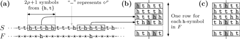
Figure 1: An example of the alignment of $F$ and $S_{t}$ at some well-aligned arrival $t$. Only a portion of the strings are shown, containing two occurrences of the h-symbol in $F$. Every substring $\diamond^{\rho}$ is illustrated with a short line segment.

Consider now the rectangular boxes stacked on top of each other as in Figure 1(b). The $i$-th box from the top corresponds to the $i$-th h-symbol in $F$. Each box contains $2\rho+1$ elements from $\{\texttt{{h}},\texttt{{t}}\}$ and may be regarded as a row of a matrix with $2\rho+1$ columns. We refer to this matrix as $M_{t}$. Observe that in the hard distribution, the entries of $M_{t}$ are drawn independently and uniformly at random from $\{\texttt{{h}},\texttt{{t}}\}$.

Define $\pi$ to be a set of matrix coordinates of h-entries of $M_{t}$, containing at most one entry from each row. Let $\Pi_{t}$ be the set of all such sets $\pi$. In Figure 1(b) and (c) we have illustrated two examples of $\pi$, where its elements are highlighted in grey. Given some $\pi$, let $h_{1},\dots,h_{|\pi|}$ denote the elements of $\pi$ in top-to-bottom order. Each set $\pi$ uniquely specifies a subsequence $C_{\pi}\in\mathcal{C}_{t}$ by describing which h-symbols are chosen from each rectangular box. The subsequence $C_{\pi}$ is then completed greedily by including as many $\diamond$-symbols as possible.

We also define $\operatorname{col}(i)\in\{1,\dots,2\rho+1\}$ to be the column in which $h_{i}$ occurs and the value $n_{\diamond}$ to be the number of $\diamond$-symbols in $F$. Observe that $n_{\diamond}$ only depends on $n$. We can now define

$$\textup{length}(\pi)=n_{\diamond}+|\pi|-\frac{\rho}{2}\cdot\Big{(}|\rho+1-\operatorname{col}(1)|+|\rho+1-\operatorname{col}(|\pi|)|+\sum_{i=1}^{|\pi-1|}|\operatorname{col}(i)-\operatorname{col}(i+1)|\Big{)}.$$

The following lemma tells us that $\textup{length}(\pi)$ is in fact the length of the common subsequence $C_{\pi}$ implied by $\pi$.

Lemma 9.

For any well-aligned arrival $t$ and any $\pi\in\Pi_{t}$, $\textup{length}(\pi)=|C_{\pi}|$.

Proof.

Let $t$ be any well-aligned arrival and let $\pi$ be any set from $\Pi_{t}$. As described above, $\pi$ uniquely specifies a common subsequence $C_{\pi}$ of $F$ and $S_{t}$. Recall that the elements of $\pi$ are denoted $h_{1},\dots,h_{|\pi|}$ in top-to-bottom order with respect to the matrix $M_{t}$. For $i\in\{0,\dots,|\pi|\}$, we define

$$\textup{columndist}(i,i+1)=\begin{cases}|\rho+1-\operatorname{col}(1)|&\textup{if $i=0$,}\\ |\rho+1-\operatorname{col}(|\pi|)|&\textup{if $i=|\pi|$,}\\ |\operatorname{col}(i)-\operatorname{col}(i+1)|&\textup{otherwise.}\end{cases}$$

We can now write $\textup{length}(\pi)$ as

$$\textup{length}(\pi)=n_{\diamond}+|\pi|-\frac{\rho}{2}\sum_{i=0}^{|\pi|}\textup{columndist}(i,i+1).$$

Referring to the above formula for $\textup{length}(\pi)$, and starting with the number $n_{\diamond}$ of $\diamond$-symbols, we will show that adding the number of h-symbols in $C_{\pi}$, that is adding the term $|\pi|$, and subtracting the other terms of the equation will indeed equal $|C_{\pi}|$. That is, we will show that the number of omitted $\diamond$-symbols in $C_{\pi}$ is exactly

$$\frac{\rho}{2}\cdot\sum_{i=0}^{|\pi|}\textup{columndist}(i,i+1).$$

Similarly to the definition of $\operatorname{col}(i)$, we define for $i\in\{1,\dots,|\pi|\}$, $\textup{row}(i)$ to be the row of $M_{t}$ in which $h_{i}$ occurs.

Let $s_{1}$ be the number of $\diamond$-symbols in $S_{t}$ to the left of the h-symbol in $S_{t}$ that correspond to $h_{1}$. Similarly, let $f_{1}$ be the number of $\diamond$-symbols in $F$ to the left of the $\textup{row}(h_{1})$-th h-symbol. Thus,

$$|f_{1}-s_{1}|=\rho\cdot\textup{columndist}(0,1).$$

Now, let

$$d_{1}=\begin{cases}\phantom{-}1&\mbox{if $f_{1}>s_{1}$},\\ -1&\mbox{otherwise.}\end{cases}$$

Thus, $d_{1}=1$ whenever $|s_{1}-f_{1}|$ $\diamond$-symbols of $F$, up to the $\textup{row}(h_{1})$-th h-symbol, are omitted from $C_{\pi}$. Otherwise, all $\diamond$-symbols of $F$ up to the $\textup{row}(h_{1})$-th h-symbol are included in $C_{\pi}$, and $d_{1}=-1$. The purpose of $d_{1}$ will be clear shortly.

Now consider $h_{i}\in\pi$ for $i\in\{2,\dots,|\pi|\}$. We will define $s_{i}$, $f_{i}$ and $d_{i}$ similarly to $s_{1}$, $f_{1}$ and $d_{1}$. That is, let $s_{i}$ be the number of $\diamond$-symbols in $S_{t}$ between the h-symbols that correspond to $h_{i-1}$ and $h_{i}$, respectively. Let $f_{i}$ be the number of $\diamond$-symbols in $F$ between the $\textup{row}(i-1)$-th and $\textup{row}(i)$-th h-symbols in $F$. Thus,

$$|f_{i}-s_{i}|=\rho\cdot\textup{columndist}(i-1,i).$$

Similarly to $d_{1}$, let

$$d_{i}=\begin{cases}\phantom{-}1&\mbox{if $f_{i}>s_{i}$},\\ -1&\mbox{otherwise.}\end{cases}$$

We have $d_{i}=1$ if $|f_{i}-s_{i}|$ $\diamond$-symbols between the $\textup{row}(i-1)$-th and $\textup{row}(i)$-th h-symbols of $F$ are omitted from $C_{\pi}$, and $d_{i}=-1$ if no such $\diamond$-symbols are omitted.

Finally, in order to capture $\diamond$-symbols to the right of the last h-symbol in $C_{\pi}$, let $s_{|\pi|+1}$ be the number of $\diamond$-symbols in $S_{t}$ to the right of the h-symbol that corresponds to $h_{\pi}$, and let $f_{|\pi|+1}$ be the number of $\diamond$-symbols in $F$ to the right of the $\textup{row}(h_{\pi})$-th h-symbol in $F$. We have

$$|f_{|\pi|+1}-s_{|\pi|+1}|=\rho\cdot\textup{columndist}(|\pi|,|\pi|+1),$$

and we let

$$d_{|\pi|+1}=\begin{cases}\phantom{-}1&\mbox{if $f_{|\pi|+1}>s_{|\pi|+1}$},\\ -1&\mbox{otherwise.}\end{cases}$$

The number $n_{\diamond}$ of $\diamond$-symbols is the same in both $F$ and $S_{t}$ and is exactly

$$n_{\diamond}=\sum_{i=1}^{|\pi|+1}f_{i}=\sum_{i=1}^{|\pi|+1}s_{i}.$$

Hence,

$$\sum_{i=1}^{|\pi|+1}(f_{i}-s_{i})=\sum_{i=1}^{|\pi|+1}d_{i}\cdot|f_{i}-s_{i}|=0,$$

where we have used the definition of $d_{i}$ from above. Separating into positive and negative terms, we have that

$$\sum_{i\,|\,d_{i}=1}|f_{i}-s_{i}|=\sum_{i\,|\,d_{i}=-1}|f_{i}-s_{i}|,$$

which we use in the next equation. The total number of $\diamond$-symbols that are omitted in $C_{\pi}$ is

$$\sum_{i\,|\,d_{i}=1}|f_{i}-s_{i}| =\frac{1}{2}\left(\sum_{i\,|\,d_{i}=1}|f_{i}-s_{i}|+\sum_{i\,|\,d_{i}=-1}|f_{i}-s_{i}|\right)$$

$$=\frac{1}{2}\sum_{i=1}^{|\pi|+1}|f_{i}-s_{i}|$$

$$=\frac{1}{2}\sum_{i=1}^{|\pi|+1}\rho\cdot\textup{columndist}(i-1,i)$$

$$=\frac{\rho}{2}\sum_{i=0}^{|\pi|}\textup{columndist}(i,i+1),$$

which is what we wanted to show. ∎

Let $\pi^{*}\in\Pi_{t}$ be the set of coordinates of all h-symbols that appear in the middle column of $M_{t}$. See Figure 1(c) for an example. The following probabilistic fact tells us that we can simply choose these symbols and still maximise $\textup{length}(\pi)$ with constant probability. The proof follows by first showing that if every $(d\times 1)$-submatrix of $M_{t}$ contains between $d/2-\rho/4$ and $d/2+\rho/4$ h-symbols then for all $\pi\in\Pi_{t},\textup{length}(\pi)\leqslant\textup{length}(\pi^{*})$. At a high level, when the number of h-symbols for all $(d\times 1)$ submatrices is within this bound one can never compensate from the cost of deviating from the middle column. We then show that $M_{t}$ has this property with probability at least $9/10$.

Lemma 10.

Let $M_{t}$ be a random matrix whose elements are chosen independently and uniformly at random from $\{\texttt{{h}},\texttt{{t}}\}$. With probability at least $9/10$, $\textup{length}(\pi)\leqslant\textup{length}(\pi^{*})$ for all $\pi\in\Pi_{t}$.

Proof.

We will drop the subscript $t$ from $M_{t}$ and $\Pi_{t}$ in the rest of the proof. Let $M$ be a random binary matrix whose elements are chosen independent and uniformly at random from $\{\texttt{{h}},\texttt{{t}}\}$. For any $\pi\in\Pi$, let $h_{1},\dots,h_{|\pi|}$ be the elements of $\pi$ in top-to-bottom order with respect to the matrix $M$. We may write $\textup{length}(\pi)$ as

$$\textup{length}(\pi)~{}=~{}n_{\diamond}+\text{val}(\pi),$$

where

$$\text{val}(\pi)~{}=~{}|\pi|-\frac{\rho}{2}\cdot\sum_{i=0}^{|\pi|}\textup{columndist}(i,i+1)$$ (1)

and $\textup{columndist}(i,i+1)$ was defined in the proof of Lemma 9. Since $n_{\diamond}$ only depends on $n$, we will show that with probability $9/10$, $\text{val}(\pi)\leqslant\text{val}(\pi^{*})$ for every $\pi\in\Pi$.

Let $\pi$ be any set in $\Pi$. There is a unique partition of $\pi$ into disjoint subsets, which we denote $\pi_{1},\dots,\pi_{m}$, such that two elements $h_{j},h_{j^{\prime}}\in\pi$, where $j<j^{\prime}$, belong to the same $\pi_{i}$ if and only if $\operatorname{col}(j)=\operatorname{col}(j+1)=\cdots=\operatorname{col}(j^{\prime})$, and further, for any two distinct elements $h_{j}\in\pi_{i}$ and $h_{j^{\prime}}\in\pi_{i^{\prime}}$, where $i<i^{\prime}$, we have $j<j^{\prime}$. As en example, the partition of $\pi^{*}$ contains only the set $\pi^{*}$ itself as all elements are from the same column.

For $i\in\{1,\dots,|\pi|\}$, let $\textup{row}(i)$ be the row of $M$ in which $h_{i}$ occurs. For any $\pi_{i}$ in the partition of $\pi$, let

$$\textup{toprow}(\pi_{i}) ~{}=~{}\min_{h_{j}\in\pi_{i}}~{}\textup{row}(j),$$

$$\textup{bottomrow}(\pi_{i}) ~{}=~{}\max_{h_{j}\in\pi_{i}}~{}\textup{row}(j),$$

$$\textup{column}(\pi_{i}) ~{}=~{}~{}\textup{the column of $M$ from which the elements of $\pi_{i}$ are.}$$

We say that $M$ is balanced if every $(d\!\times\!1)$-submatrix of $M$ (one column wide and height $d$) contains at least $d/2-\rho/4$ and at most $d/2+\rho/4$ h-symbols. We will first show that if $M$ is balanced then $\text{val}(\pi)\leqslant\text{val}(\pi^{*})$ for every $\pi\in\Pi$. Then we will show that a random $M$ is balanced with probability $9/10$.

So, suppose that $M$ is balanced. Let $n_{\texttt{{h}}}$ be the number of h-symbols in $F$, that is the height of $M$. By considering the entire middle column of $M$, we have

$$\frac{n_{\texttt{{h}}}}{2}-\frac{\rho}{4}~{}\leqslant~{}|\pi^{*}|=\text{val}(\pi^{*}).$$ (2)

Let $\pi$ be any set in $\Pi$ and let $\pi_{1},\dots,\pi_{m}$ be the subsets in the partition of $\pi$. For $i\in\{1,\dots,m\}$, suppose $\pi_{i}=\{h_{j_{i}},\dots,h_{j^{\prime}_{i}}\}$. We define the cost of $\pi_{i}$ to be

$$\textup{cost}(\pi_{i})~{}=~{}\frac{\rho}{2}\cdot\sum_{k=j_{i}}^{j^{\prime}_{i}}\textup{columndist}(k,k+1).$$

The value $\text{val}(\pi)$ in Equation (1) can be split into $m+1$ terms of which $m$ terms correspond to the contribution from the $m$ subsets $\pi_{i}$. That is,

$$\text{val}(\pi)~{}=\;-\frac{\rho}{2}\cdot\textup{columndist}(0,1)+\sum_{i=1}^{m}\big{(}|\pi_{i}|-\textup{cost}(\pi_{i})\big{)},$$

Let the height of the subcolumn spanned by elements from $\pi_{i}$ be

$$d_{i}~{}=~{}\textup{bottomrow}(\pi_{i})-\textup{toprow}(\pi_{i})+1.$$

Then, since $M$ is balanced,

$$|\pi_{i}|~{}\leqslant~{}\frac{d_{i}}{2}+\frac{\rho}{4}.$$

Thus,

$$\text{val}(\pi) ~{}\leqslant\;-\frac{\rho}{2}\cdot\textup{columndist}(0,1)+\sum_{i=1}^{m}\left(\frac{d_{i}}{2}+\frac{\rho}{4}-\textup{cost}(\pi_{i})\right)$$

$$~{}\leqslant~{}\frac{n_{\texttt{{h}}}}{2}-\frac{\rho}{2}\cdot\textup{columndist}(0,1)+\sum_{i=1}^{m}\left(\frac{\rho}{4}-\textup{cost}(\pi_{i})\right)$$ (3)

since $\sum_{i=1}^{m}d_{i}$ is at most the number of rows $n_{\texttt{{h}}}$ of $M$.

In order to show that $\text{val}(\pi)\leqslant\text{val}(\pi^{*})$, first consider the case where $m=1$. Then there is only one set in the partition of $\pi$ and it follows immediately by Equation (1) that $\text{val}(\pi)\leqslant\text{val}(\pi^{*})$.

In the case $m=2$, suppose first that $\textup{column}(\pi_{1})$ is the middle column of $M$. Then an upper bound on Inequality 3 is given by

$$\frac{n_{\texttt{{h}}}}{2}-\frac{\rho}{2}\cdot 0+\left(\frac{\rho}{4}-\frac{\rho}{2}\right)~{}=~{}\frac{n_{\texttt{{h}}}}{2}-\frac{\rho}{4}~{}\leqslant~{}\text{val}(\pi^{*}),$$

where the last inequality uses Inequality (2). The case where $\textup{column}(\pi_{1})$ is not the middle column of $M$ is similar as $\textup{columndist}(0,1)$ is then at least 1.

Finally, in the case where $m\geqslant 3$, first observe that $\textup{cost}(\pi_{i}$) is at least $\rho/2$ for all $\pi_{i}$ except for possibly $\pi_{m}$ if $\textup{column}(\pi_{m})$ is the middle column of $M$. An upper bound on Inequality 3 is given by

$$\frac{n_{\texttt{{h}}}}{2}-\frac{\rho}{2}\cdot 0+(m-1)\cdot\left(\frac{\rho}{4}-\frac{\rho}{2}\right)+\left(\frac{\rho}{4}-0\right)~{}=~{}\frac{n_{\texttt{{h}}}}{2}-(m-2)\cdot\frac{\rho}{4}~{}\leqslant~{}\frac{n_{\texttt{{h}}}}{2}-\frac{\rho}{4}~{}\leqslant~{}\text{val}(\pi^{*}),$$

We will now show that if $M$ is random, then with probability at least $9/10$, $M$ is balanced. Consider a arbitrary $(d\!\times\!1)$-submatrix of $M_{t}$. The number of h-entries in this submatrix is binomially distributed with parameter $(d,\frac{1}{2})$. Thus, by Hoeffding’s inequality we have that the probability that there are less than $(d/2-\rho/4)$ h-entries in this submatrix is at most

$$e^{{\frac{-2(\rho/4)^{2}}{d}}}~{}<~{}e^{{\frac{-4\log n\cdot\log\log n}{\log n}}}~{}\leqslant~{}\frac{1}{\log^{4}n},$$

where the second inequality follows because the height of $M$ is at most $\log n$ and the value of $\rho=4\sqrt{\log n\cdot\log\log n}$. By symmetry, this is also an upper bound on the probability that there are more than $(d/2+\rho/4)$ h-entries in the submatrix. Thus, $2/\log^{4}n$ is an upper bound on the probability that the number of h-entries is not in the range $d/2\pm\rho/4$.

By the union bound over all $(d\!\times\!1)$-submatrices of $M$ it follows that the probability that $M$ is balanced is at least $9/10$ for sufficiently large $n$. To see this, recall that the width of $M$ is $2\rho+1\leqslant\log n$, hence there are at most $\log^{3}n$ submatrices of width 1. ∎

Finally we can prove that in the hard instance for the LCS problem, at any well-aligned arrival $t$, $\textup{LCS}(F,S_{t})=n-\textup{Ham}(F,S_{t})$ with probability at least $9/10$ and hence establish Lemma 5.

Proof of Lemma 5.

By combining Lemma 8 with Lemma 9 we have that $\max_{\pi\in\Pi_{t}}\textup{length}(\pi)=\textup{LCS}(F,S_{t})$, thus by Lemma 10 we have that $\textup{length}(\pi^{*})=\textup{LCS}(F,S_{t})$ with probability at least $9/10$. The desired result follows from the observation that $\textup{length}(\pi^{*})=|C_{\pi^{*}}|=n-\textup{Ham}(F,S_{t})$. ∎

6 A lower bound for the information transfer

We are now able to prove Lemma 3 which gives us lower bounds for the expected size of the information transfer of a node. Our approach extends that of Pǎtraşcu and Demaine from [17]. Let $v$ be a node of the information transfer tree $\mathcal{T}$ and recall that the expected length of any encoding of the outputs $Y_{v}$ is an upper bound on its entropy. Pǎtraşcu and Demaine showed that it is possible to bound the conditional entropy of $Y_{v}$ in terms of the expected information transfer size $\mathbb{E}[I_{v}]$ by using what we will call an address-based encoding scheme. A shortcoming of this encoding, which we will have to overcome, is that storing the address of a cell could require $\Theta(\log n)$ bits, making the length of the encoding too large to be useful for small $w$, that is $w\in o(\log n)$. In the following lemma we have slightly generalised the original statement of this bound from [17] to make the role that the word size $w$ plays explicit.

Lemma 11 (Pǎtraşcu and Demaine [17]).

There is a positive constant $\alpha$ such that for any node $v$ of the information transfer tree $\mathcal{T}$, the entropy

$$H(Y_{v}\mid\widetilde{\mathcal{S}}_{v}=\widetilde{s}_{v})~{}\leqslant~{}(w+\alpha\cdot\log n)\cdot\mathbb{E}\left[I_{v}\bigm{|}\widetilde{\mathcal{S}}_{v}=\widetilde{s}_{v}\right].$$

Towards a new encoding that circumvents the limitations of Lemma 11 we propose, as an intermediate step, another encoding which is used to prove the following lemma. We refer to this encoding as the counting-based encoding.

Lemma 12.

For any node $v$ of the information transfer tree $\mathcal{T}$, the entropy

$$H(Y_{v}\mid\widetilde{\mathcal{S}}_{v}=\widetilde{s}_{v})~{}\leqslant~{}\mathbb{E}\left[\log{R_{v}\choose I_{v}}+w\cdot I_{v}+\log I_{v}~{}\Bigm{|}~{}\widetilde{\mathcal{S}}_{v}=\widetilde{s}_{v}\right].$$

Proof.

We keep a counter of the cell reads performed by any correct algorithm for our online problems. For each cell $c\in\mathcal{I}_{v}$, we store the contents of $c$ and the value of the cell-read counter for when $c$ is read for the first time during the time interval in which $Y_{v}$ is outputted. To see why this encodes $Y_{v}$, under a fixed $\widetilde{\mathcal{S}}_{v}$, we use the algorithm as a decoder. That is, first run the algorithm on known inputs until the first symbol in $\mathcal{S}_{v}$ arrives. Then skip over all inputs in $\mathcal{S}_{v}$ and start simulating the algorithm from the beginning of the interval where $Y_{v}$ is outputted. For every cell $c$ being read, use the cell-read counter to determine whether $c$ is in $\mathcal{I}_{v}$ or not. If it is, read its contents from the encoding of $\mathcal{I}_{v}$, otherwise we already have the correct value from running the algorithm on $\widetilde{\mathcal{S}}_{v}$.

The cell-read counter and contents of the cells in $\mathcal{I}_{v}$ can be encoded succinctly as follows. During the time interval in which the algorithm outputs $Y_{v}$, there are ${R_{v}\choose I_{v}}$ possible scenarios of when the cells in $\mathcal{I}_{v}$ are read for the first time. Thus, under a predefined enumeration of these scenarios, we can specify in exactly $\log{R_{v}\choose I_{v}}$ bits when each cell in $\mathcal{I}_{v}$ is read. To do so we would also need to encode the size of $\mathcal{I}_{v}$, which can be done in $\log I_{v}$ bits. The contents of the cells in $\mathcal{I}_{v}$ is encoded in a total of $w\cdot I_{v}$ bits and stored sorted by the time of the cell read. Observe that it suffices to store only the first read of any cell in $\mathcal{I}_{v}$ as the decoder remembers every cell it has already accessed. ∎

To obtain our new lower bound for $\mathbb{E}[I_{v}]$ we will combine these two encodings schemes. More precisely, let $r_{v}=\ell_{v}\cdot\delta\cdot\log^{2}n$ define a threshold value. When $R_{v}\geqslant r_{v}$, we use the address-based encoding, and when $R_{v}<r_{v}$ we use the counting-based encoding. The threshold has been chosen carefully so that we utilise the strengths of each of the two encodings. Only one bit of additional information is required to specify which of the two encodings is used.

We now use the fact that Lemma 3 only relates to fast nodes $v$ and use a combination of the two encodings and the fact that $v$ is either a high-entropy or a medium-entropy node. This gives us both upper and lower bounds on the conditional entropy of $Y_{v}$ which after some manipulation will provide us with our desired lower bounds for $\mathbb{E}[I_{v}]$.

Proof of Lemma 3.

We begin by proving the Hamming distance and convolution part of the lemma when $w\geqslant\log n$. In this case, the bound in the statement of the lemma simplifies to

$$\mathbb{E}[I_{v}]\in\Omega{\left(\frac{\delta\cdot\ell_{v}}{w}\right)}.$$

Regardless of whether the node $v$ is fast or not, this lower bound on $\mathbb{E}[I_{v}]$ has already been established in previous work [3, 4] by using the address-based encoding. In the rest of the proof we will therefore focus on the case where $w<\log n$. Here the concept of a fast node will be important.

The encoding we use when $w<\log n$ is a combination of the address-based encoding of Lemma 11 and the new counting-based encoding of Lemma 12. We refer to this combined encoding as the mixed encoding. Let

$$r_{v}=\ell_{v}\cdot\delta\cdot\log^{2}n$$

be a threshold value such that when $R_{v}\geqslant r_{v}$ we use the address-based encoding, and when $R_{v}<r_{v}$ we use the counting-based encoding. The threshold has been chosen carefully so that we utilise the strengths of each one of the two encodings. One single bit of information is sufficient to specify which encoding is being used.

Suppose $v$ is a high-entropy node when proving the Hamming distance and convolution part of the lemma, and suppose $v$ is a medium-entropy node when proving the edit distance and LCS part. The proof is almost identical for both parts so we will combine them as follows. Let

$$f(n)=\begin{cases}\frac{1}{2}\cdot k&\mbox{when proving the Hamming distance and convolution part,}\\ \frac{1}{2}\cdot\frac{k}{\sqrt{\log n\cdot\log\log n}}&\mbox{when proving the edit distance and LCS part,}\end{cases}$$

where $k$ is the constant from either Definition 1 of a high-entropy node or Definition 2 of a medium-entropy node, respectively. Thus,

$$H(Y_{v}\mid\widetilde{\mathcal{S}}_{v}=\widetilde{s}_{v})\,\geqslant\,2\cdot f(n)\cdot\delta\cdot\ell_{v},$$ (4)

where $\widetilde{s}_{v}$ is a fixed value. Observe the factor $1/2$ in $f(n)$. It is included for convenience as will be clear shortly. Recall that by Definition 2 of a medium-entropy node $v$, Inequality (4) is only guaranteed to hold for half of the fixed values $\widetilde{s}_{v}$.

Let the random variable $Z_{v}$ denote the size of the mixed encoding of $Y_{v}$. Since the expected size of any encoding is an upper bound on the entropy,

$$\mathbb{E}[Z_{v}\mid\widetilde{\mathcal{S}}_{v}=\widetilde{s}_{v}]\,\geqslant\,H(Y_{v}\mid\widetilde{\mathcal{S}}_{v}=\widetilde{s}_{v}).$$

Since $\widetilde{\mathcal{S}}_{v}$ is chosen uniformly from all possible instances in the hard distribution for all our problems, taking expectation over $\widetilde{\mathcal{S}}_{v}$, gives

$$\mathbb{E}[Z_{v}]\geqslant f(n)\cdot\delta\cdot\ell_{v}.$$ (5)

Here the factor $1/2$ in the definition of $f(n)$ comes in handy as Inequality (4) is only guaranteed to hold for half of the values of $\widetilde{\mathcal{S}}_{v}$ in the definition of a medium-entropy node $v$.

The goal is to derive a lower bound on $\mathbb{E}[I_{v}]$. We condition on the running time $R_{v}$:

$$\mathbb{E}[Z_{v}]~{}=~{}\Pr[R_{v}\geqslant r_{v}]\cdot\mathbb{E}[Z_{v}\mid R_{v}\geqslant r_{v}]~{}+~{}\Pr[R_{v}<r_{v}]\cdot\mathbb{E}[Z_{v}\mid R_{v}<r_{v}].$$ (6)

We will upper bound $\mathbb{E}[Z_{v}]$ by upper bounding each term on the right hand side separately, starting with the first term. By the definition of a fast node,

$$\mathbb{E}[R_{v}]\,\leqslant\,\ell_{v}\cdot\delta\cdot\log n.$$

Using Markov’s inequality, it follows that

$$\Pr[R_{v}\geqslant r_{v}]\,\leqslant\,\frac{1}{\log n}.$$

Whenever $R_{v}\geqslant r_{v}$, the address-based encoding is used, for which

$$Z_{v}\,\leqslant\,(\alpha+1)\cdot\log n\cdot I_{v},$$

where $\alpha$ is the constant of Lemma 11 and $w\leqslant\log n$. From the last two inequalities we conclude that the first term of Equation (6) is upper bounded by $(\alpha+1)\cdot\mathbb{E}[I_{v}]$.

We now upper bound the second term of Equation (6). Trivially, $\Pr[R_{v}<r_{v}]\leqslant 1$. When $R_{v}<r_{v}$, the counting-based encoding of Lemma 12 is used, hence

$$Z_{v}\,=\,\log{R_{v}\choose I_{v}}+w\cdot I_{v}+\log I_{v}\,\leqslant\,2\left(\log{R_{v}\choose I_{v}}+w\cdot I_{v}\right).$$

Using the fact ${a\choose b}\leqslant(a\cdot e/b)^{b}$ and the conditioning $R_{v}<r_{v}$, we have

$$Z_{v} \,\leqslant\,2(I_{v}\log r_{v}+I_{v}\log e-I_{v}\log I_{v}+w\cdot I_{v})$$

$$\,=\,2I_{v}\log r_{v}+I_{v}\cdot k_{1}w-2I_{v}\log I_{v},$$

where $k_{1}=2+2\log e$ is a constant. Thus, by linearity of expectation,

$$\mathbb{E}[Z_{v}\mid R_{v}<r_{v}]\,\leqslant\,\mathbb{E}[I_{v}]\cdot 2\log r_{v}+\mathbb{E}[I_{v}]\cdot k_{1}w+\mathbb{E}[-2I_{v}\cdot\log I_{v}],$$

where the last term is concave and therefore, by Jensen’s inequality, upper bounded by

$$\mathbb{E}[I_{v}]\cdot(-2\log\mathbb{E}[I_{v}]),$$

which gives us

$$\mathbb{E}[Z_{v}\mid R_{v}<r_{v}]\,\leqslant\,\mathbb{E}[I_{v}]\cdot\big{(}2\log r_{v}+k_{1}w-2\log\mathbb{E}[I_{v}]\big{)}.$$

Using the upper bounds on the terms of Equation (6) that we just derived, combined with the lower bound on $\mathbb{E}[Z_{v}]$ of Inequality (5), as well as substituting $r_{v}$ with its value $\ell_{v}\cdot\delta\cdot\log^{2}n$, we have

$$(\alpha+1)\cdot\mathbb{E}[I_{v}]+\mathbb{E}[I_{v}]\cdot\big{(}2\log\ell_{v}+2\log\delta+4\log\log n+k_{1}w-2\log\mathbb{E}[I_{v}]\big{)}$$

$$\geqslant~{}f(n)\cdot\delta\cdot\ell_{v}$$

or equivalently,

$$\mathbb{E}[I_{v}] \,\geqslant\,\frac{f(n)\cdot\delta\cdot\ell_{v}}{(\alpha+1)+2\log\ell_{v}+2\log\delta+4\log\log n+k_{1}w-2\log\mathbb{E}[I_{v}]}$$

$$\,\geqslant\,\frac{\frac{1}{2}f(n)\cdot\delta\cdot\ell_{v}}{\log\ell_{v}+\log\delta+2\log\log n+k_{2}w-\log\mathbb{E}[I_{v}]},$$ (7)

where $k_{2}=(a+1)+k_{1}$ is a constant. In order to lower bound $\mathbb{E}[I_{v}]$ it might be tempting to set the $-\log\mathbb{E}[I_{v}]$ term to zero in the denominator above. Unfortunately, this bound will be too weak for our purposes. Instead we perform the following arithmetic manoeuvre.

First observe that if $\mathbb{E}[I_{v}]$ is so large that the denominator of Inequality (7) is negative then the statement of Lemma 3 follows by a suitable choice of constants. We therefore continue under the assumption that the denominator is positive.

In the hard distribution for Hamming distance and convolution, observe that by Lemma 1, the information transfer $\mathcal{I}_{v}$ must always contain at least one cell. Similarly by Lemma 2, in the hard distribution for edit distance and LCS, for at least half of the fixed values of $\widetilde{\mathcal{S}}_{v}$ the information transfer contains at least one cell. Thus,

$$\mathbb{E}[I_{v}]\geqslant\frac{1}{2}.$$

By replacing the $\log\mathbb{E}[I_{v}]$ term in the denominator of Inequality (7) with $-1$ we get a lower bound on $\mathbb{E}[I_{v}]$. We use $L$ as a shorthand for this lower bound, hence

$$\mathbb{E}[I_{v}]\,\geqslant\,L\,=\,\frac{\frac{1}{2}f(n)\cdot\delta\cdot\ell_{v}}{\log\ell_{v}+\log\delta+2\log\log n+k_{3}w}\,,$$

and $k_{3}=k_{2}+1$, implying $k_{3}w\geqslant k_{2}w+1\geqslant k_{2}w-\log\mathbb{E}[I_{v}]$.

We can now boost the lower bound $L$ of $\mathbb{E}[I_{v}]$ by reconsidering Equation (7) and replacing the $-\log\mathbb{E}[I_{v}]$ term in the denominator with $-\log L$. That is,

$$\mathbb{E}[I_{v}]\,\geqslant\,\frac{\frac{1}{2}f(n)\cdot\delta\cdot\ell_{v}}{\log\ell_{v}+\log\delta+2\log\log n+k_{2}w-\log L}\,.$$ (8)

By substituting $L$ with its value above, the denominator in Inequality (8) can be written as

$$\log\ell_{v}+\log\delta+2\log\log n+k_{2}w-\log(\frac{1}{2}f(n)\cdot\delta\cdot\ell_{v})$$

$$\phantom{=\,}+\log(\log\ell_{v}+\log\delta+2\log\log n+k_{3}w)$$

$$\leqslant\log\ell_{v}+\log\delta+2\log\log n+k_{2}w-\log\frac{1}{2}-\log f(n)-\log\delta-\log\ell_{v}$$

$$\phantom{=\,}+\log(\log n+\log n+2\log n+k_{3}\log n) w\leqslant\log n$$ (recall )

$$\leqslant 3\log\log n+k_{4}w-\log f(n)$$

$$\leqslant 4\log\log n+k_{5}w\,,$$

where $k_{4}$ and $k_{5}$ are constants, and where the last inequality holds for either value of $f(n)$ above. We have also assumed that $\delta\leqslant n$, that is we ignore the unnatural case where inputs are exponential in $n$. Thus, by substituting the upper bound on the denominator into Equation (8), we have

$$\mathbb{E}[I_{v}]\,\geqslant\,\frac{f(n)\cdot k_{6}\cdot\delta\cdot\ell_{v}}{w+\log\log n}\,,$$

where $k_{6}$ is yet another constant. This inequality concludes the argument we need to prove Lemma 3. For Hamming distance and convolution the result now follows immediately and for the edit distance and LCS we simply set $\delta=2$ and $w=1$. ∎

7 A cell-probe algorithm for the edit distance problem

In this section we prove Theorem 3, that is we show that there is a cell-probe algorithm that solves the online edit distance problem and runs in $O((\log^{2}n)/w)$ amortised time per arriving symbol. We want the algorithm to output

$$d(i)=\min_{h\leqslant i}\,\textup{Edit}(F,S[h,i]),$$ (9)

where $F$ is the fixed string of length $n$, $S$ is the stream, and $\textup{Edit}(F,S[h,i])$ is the smallest number of edit operations (i.e., replace, delete and insert) required to transform $F$ into the substring $S[h,i]$. Recall that at arrival $i$, only the symbols in $S[0,i]$ are known to the algorithm. That is, the algorithm cannot know what symbols will arrive in the future.

7.1 Three assumptions

We make three assumptions about the input in order to make the presentation of our algorithm cleaner. The first assumption is about the alphabet size. The symbols in both $F$ and $S$ are from the alphabet $[2^{\delta}-1]$ and we will assume that $2^{\delta}\leqslant n+1$, hence $\delta\in O(\log n)$. As there can be at most $n$ distinct symbols in $F$, if the alphabet contains more than $n+1$ symbols we can map every symbol not in $F$ to one specific symbol that does not occur in $F$. This mapping can easily be done in $O(\delta)$ time, or $O(\log n$) time, if the alphabet size is polynomial in $n$.

Secondly we assume that $n$ is a power-of-two. It is easy to extend our algorithm to allow any $n$. Namely, pad $F$ at the left-hand end with a new symbol $\sigma$, where $\sigma$ does not occur in $S$, such that the length increases from $n$ to $n^{\prime}$, where $n^{\prime}$ is the smallest power-of-two greater than $n$. Call this new string $F^{\prime}$. Adding the symbol $\sigma$ increases the alphabet size by one, hence increases $\delta$ by at most one. Now observe that

$$\text{Edit}(F,S[h,i])=\text{Edit}(F^{\prime},S[h,i])-(n^{\prime}-n).$$

Thus, we solve the online edit distance problem for $F^{\prime}$ and simply subtract $n^{\prime}-n$ from every output.

Lastly we will assume that the fixed array $F$ is known to the algorithm, that is, for an arbitrarily given $F$ of length $n$ we show that there is an algorithm that solves the edit distance problem such that the algorithm performs on average $O((\log^{2}n)/w)$ cell probes per symbol arrival. By “hard-coding” $F$ into the algorithm we avoid charging for cell probes when accessing elements of $F$. In Section 7.6 we explain how this constraint can be lifted by adding a preprocessing stage of $F$ before the symbols start arriving in the stream. Thus, ultimately we do indeed give an algorithm that takes both $F$ and the stream $S$ as input. The preprocessing uses a super-polynomial number of cell probes.

7.2 Dynamic programming and the underlying DAG

The offline edit distance problem is traditionally solved with dynamic programming by filling in a two-dimensional programming table. The dynamic programming recurrence specifies a directed acyclic graph (DAG) such that the optimal sequence of edit operations can be obtained by tracing the edges backwards. We will simply refer to this graph as the DAG, where the nodes form a two-dimensional lattice. The nodes are labelled $(j,i)$, where $j\in\{-1\}\cup[n]$ is the row and $i\in\{-1\}\cup\mathbb{N}$ is the column. The rows are associated with the fixed string $F$ such that row $j$ is associated with $F[j]$. Row $-1$ is not associated with any symbol of $F$ but is there two allow the empty string. Similarly, the columns are associated with the stream $S$ such that column $i$ is associated with $S[i]$. Column $-1$ is not associated with any symbol of $S$. Observe that the width of the DAG is unlimited and grows as new symbols arrive.

The edges of the DAG have weights from the set $\{0,1\}$ to reflect the dynamic programming recurrence. Node $(j,i)$ has the following three edges leaving it: [$\qquad\rightarrow$] Edge $((j,i),(j,i+1))$. Weight is always 1 except when $j=-1$ in which case the weight is 0.

Edge $((j,i),(j+1,i))$. Weight is always 1.

Edge $((j,i),(j+1,i+1))$. Weight is 0 if $F[j+1]=S[i+1]$ and 0 otherwise. We define $\operatorname{ED}(j,i)$ to be the weight of the smallest-weight path from $(-1,-1)$ to $(j,i)$ in the DAG. It follows that

$$d(i)=\operatorname{ED}(n-1,i),$$

where $d(i)$, defined in Equation (9), is the output after the $i$-th arrival in the stream.

We will use the variable name $j$ exclusively to point to elements of $F$ and wherever we write for all $j$ we mean for all $j\in\{-1\}\cup[n]$. The variable name $i$ will be used to point to symbols of the stream $S$.

7.3 An algorithm for online edit distance

Towards proving Theorem 3 we first present an unoptimised algorithm that solves the online edit distance problem. In Section 7.5 we describe an important speedup that enables us to give the final time complexity of $O((\log^{2}{n})/w)$ time per arriving symbol.

Our first algorithm for computing edit distance online is given in Algorithm 1, and will be explained below. The algorithm fills in values from a dynamic programming table, denoted $D$, by reading in values from previous columns. In this respect the overall structure is similar to the classic offline dynamic programming solution for edit distance. In the standard dynamic programming solution new values are computed using values from the immediately preceding column, which is equivalent to setting $\rho(i)=i-1$ in Algorithm 1. Unfortunately, doing this would lead to a complexity of $\Omega(n/w)$ per arriving symbol. To achieve a much faster solution we will need to choose a more suitable column, modify the definition of the classic dynamic programming table and then show how its values can be succinctly encoded to allow them to be read and written efficiently.

Algorithm 1   Online edit-distance in the cell-probe model (unoptimised version)

When a new symbol $S[i]$ arrives,

• if $i=0$, compute $D(j,0)$ naively for all $j$ and output $D(n-1,0)$.

• if $i>0$, do the following.

  1. Read in the substring $S[\rho(i),i-1]$.

  2. We now know the part of the DAG spanned by the columns $\rho(i)$ through $i$ as the whole of $F$ is always known to the algorithm.

  3. Read in $D(j,\rho(i))$ for all $j$. These values are stored as blocks.

  4. Compute $D(j,i)$ for all $j$ and write these values to memory as blocks.

  5. Output $D(n-1,i)$.

For a positive integer $i$, let $\textup{predecessor}(i)$ be the number obtained by taking the binary representation of $i$ and setting the least significant 1 to 0. For example, if $i=212,$ that is $11010100$ in binary, then $\textup{predecessor}(i)=208$ as this is $11010000$ in binary. Let

$$\rho(i)=\begin{cases}\textup{predecessor}(i)&\textup{if $\textup{predecessor}(i)>i-n$,}\\ i-n&\textup{otherwise.}\end{cases}$$

When computing entries of the $i$-th column of the table, values from column $\rho(i)$ will be used. The function $\rho(i)$ specifies a column in the past and its definition ensures that we never look more than $n$ columns back. We also define $\rho_{1}(i)=\rho(i)$ and for $k\geqslant 2$, $\rho_{k}(i)=\rho(\rho_{k-1}(i))$. These iterated definitions will be useful for the analysis of our algorithm.

Let $\left\|(j,i)\rightsquigarrow(j^{\prime},i^{\prime})\right\|$ denote the smallest weight of all paths in the DAG that go from node $(j,i)$ to $(j^{\prime},i^{\prime})$, and if no such path exists, we define $\left\|(j,i)\rightsquigarrow(j^{\prime},i^{\prime})\right\|=\infty$.

We define the value $D(j,i)$ recursively. We first give the base case, then introduce some supporting notation, and finally give the recursive part of the definition.

Definition 4 (Base case).

$D(j,0)=\operatorname{ED}(j,0)$ for all $j$.

In order to define $D(j,i)$ for $i>0$, as an intermediate step we first define

$$\widetilde{D}(j,i)=\min_{j^{\prime}\in\{-1,\dots,n-1\}}\Big{(}D\big{(}j^{\prime},\rho(i)\big{)}+\left\|(j^{\prime},\rho(i))\rightsquigarrow(j,i)\right\|\Big{)}$$ (10)

and observe that that $\widetilde{D}(j,i)$ is not always finite.

We say that a sequence of positive integers in strictly decreasing order, where the difference between two consecutive numbers is 1, is a block. Any sequence of positive integers can be decomposed into consecutive blocks, for example, decomposing $9,8,7,7,6,5,4,3,4,3,2$ requires 3 blocks. The first block is $9,8,7$, the second is $7,6,5,4,3$ and the third is $4,3,2$.

For $j=n-1$ down to $-1$, the sequence of finite values $\widetilde{D}(j,i)$ can be encoded greedily as a sequence of blocks. For example, suppose that

$$\widetilde{D}(n-1,i) ,\dots,\widetilde{D}(-1,i)=$$

$$\underbrace{18,17,16,15}_{1},\underbrace{15,14,13,12,11,10,9}_{2},\underbrace{10,9,8,7}_{3},\underbrace{7,6,5,4}_{4},\infty,\dots,\infty.$$

Here we have enumerated the blocks 1, 2, 3 and 4. We let $\textup{block}(j,i)$ denote the block number that contains the value $\widetilde{D}(j,i)$. Thus, in the example above, $\textup{block}(n-1,i)=1$, $\textup{block}(n-11,i)=2$ and $\textup{block}(n-12,i)=3$. To avoid splitting into two cases, depending on whether $\widetilde{D}(j,i)$ is finite or infinite, we will refer to a sequence of $\infty$-values as a block as well. Thus, in the example above, $\textup{block}(j,i)=5$ for all $j\leqslant n-20$.

Definition 5 (Recursive part).

For $i>0$,

$$D(j,i)=\begin{cases}\widetilde{D}(j,i)&\mbox{if $\textup{block}(j,i)\leqslant 3(i-\rho(i))$,}\\ \infty&\mbox{otherwise.}\end{cases}$$

Thus, $D(j,i)$ is finite only if $\widetilde{D}(j,i)$ is contained within the first $3(i-\rho(i))$ blocks. For any $i$, this allows us to store $D(j,i)$ for all $j$ in $O((i-\rho(i))\cdot\log n)$ bits.

Before we analyse Algorithm 1 we will take a look at Figure 2 which illustrates some of the values $D(j,i)$ computed by the algorithm.

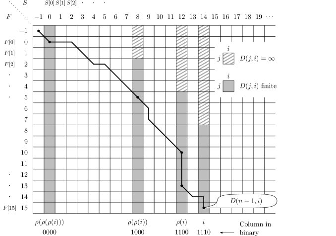
Figure 2: An example of values $D(j,i)$ computed by Algorithm 1. The path from $(-1,-1)$ to $(15,14)$ is a smallest-weight path.

Suppose that $i=14$ and symbol $S[i]$ has just arrived. Here $\rho(i)=12$, hence column 12 will be used in order to compute the values $D(j,14)$. Similarly, when computing the values $D(j,12)$, column $\rho(\rho(i))=8$ is used, and so on. By the definition of $D(j,i)$ it follows that all infinite values of a column must occur in sequence at the very top of the column. The figure illustrates a path from node $(-1,-1)$ to $(n-1,i)$ that yields the value $D(n-1,i)$. As part of the correctness analysis we will demonstrate that this path always coincides with a smallest-weight path from $(-1,-1)$ to $(n-1,i)$ in the standard dynamic programming table that solves the edit distance problem. That is, despite setting some values of the dynamic programming table to infinity, there are always sufficiently many finite values left in order to correctly compute the output.

7.4 Analysis of Algorithm 1 for online edit distance

To prove correctness of Algorithm 1 we need to show that $D(n-1,i)=\operatorname{ED}(n-1,i)$ for all $i$. We begin by proving a useful, stronger fact that holds for certain values of $i$.

Lemma 13.

For any $i$ such that $D(j,i)$ is finite for all $j$, $D(j,i)=\operatorname{ED}(j,i)$ for all $j$.

Proof.

Let $i_{r}$ denote the $r$-th column $i$ for which $D(j,i)$ is finite for all $j$. We use strong induction on $r$. For the base case $r=1$, the column is 0 and the claim is true by Definition 4.

For the induction step, suppose that the claim is true for all $i_{1},i_{2},\dots,i_{r}$ and suppose that $D(j,i_{r+1})$ is finite for all $j$. By Definition 5,

$$D(j,i_{r+1})=\widetilde{D}(j,i_{r+1})$$

for all $j$. We will show that

$$\widetilde{D}(j,i_{r+1})=\operatorname{ED}(j,i_{r+1}).$$ (11)

Observe that for any $i$ and $j$, if $D(j,i)$ is finite then so is $D(j+1,i)$. Since $\widetilde{D}(-1,i_{r+1})$ is finite, by Equation (10), $D(-1,\rho(i_{r+1}))$ is finite, hence $D(j,\rho(i_{r+1}))$ is finite for all $j$. By the induction hypothesis,

$$D(j,\rho(i_{r+1}))=\operatorname{ED}(j,\rho(i_{r+1}))$$

for all $j$. Thus, by Equation (10), Equation (11) holds for all $j$. ∎

Before showing that $D(n-1,i)=\operatorname{ED}(n-1,i)$ for all $i$ we give a property of smallest-weight paths in the DAG.

Lemma 14.

For any $i\geqslant i^{\prime}$ and $j\geqslant j^{\prime}$, no smallest-weight path from $(-1,-1)$ to $(j,i)$ can go via the node $(j^{\prime},i^{\prime})$ if

$$\operatorname{ED}(j^{\prime},i^{\prime})~{}>~{}\operatorname{ED}(j,i^{\prime})-(j-j^{\prime})+2(i-i^{\prime}).$$ (12)

Proof.

Let $P$ be any path in the DAG from $(-1,-1)$ to $(j,i)$ that passes through $(j^{\prime},i^{\prime})$. The weight of $P$ is at least

$$\operatorname{ED}(j^{\prime},i^{\prime})+(j-j^{\prime})-(i-i^{\prime}).$$ (13)

To see this, first observe that the fact is immediately true if $(j-j^{\prime})\leqslant(i-i^{\prime})$. For $(j-j^{\prime})>(i-i^{\prime})$, observe that any path from $(-1,-1)$ to $(j,i)$ via $(j^{\prime},i^{\prime})$ can contain at most $(i^{\prime}-i)$ diagonal edges of weight zero between $(j^{\prime},i^{\prime})$ and $(j,i)$.

Now suppose that Inequality (12) holds for $P$. We will show that $P$ cannot be a smallest-weight path from $(-1,-1)$ to $(j,i)$. By combining Inequality (12) with (13) we have that the weight of $P$ is strictly greater than

$$\Big{(}\operatorname{ED}(j,i^{\prime})-(j-j^{\prime})+2(i-i^{\prime})\Big{)}+(j-j^{\prime})-(i-i^{\prime})\,=\,\operatorname{ED}(j,i^{\prime})+(i-i^{\prime}).$$

To see why $P$ cannot be a smallest-weight path, consider the path $P^{\prime}$ that goes from $(-1,-1)$ to $(j,i)$ via the node $(j,i^{\prime})$. The weight of $P^{\prime}$ is at most

$$\operatorname{ED}(j,i^{\prime})+(i-i^{\prime})$$

as we can take a smallest-weight path from $(-1,-1)$ to $(j,i)$ and then follow $(i-i^{\prime})$ horizontal edges to $(i,j)$. Thus, the weight of $P^{\prime}$ is less than the weight of $P$. ∎

We can now prove that the output from Algorithm 1 is correct.

Lemma 15.

For all $i$, $D(n-1,i)=\operatorname{ED}(n-1,i)$.

Proof.

Let $P$ be any smallest-weight path from $(-1,-1)$ to $(n-1,i)$ in the DAG. Figure 3 illustrates an example of $P$ and might be helpful when going through the proof. The proof is by contradiction. Therefore, suppose that the Lemma is not true for $i$.

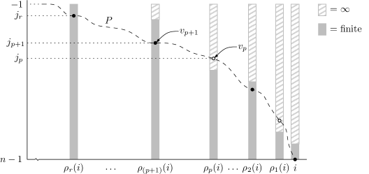
Figure 3: Here $P$ is a smallest-weight path from $(-1,-1)$ to $(n-1,i)$.

By Lemma 13, $D(j,i)$ cannot be finite for all $j$, otherwise we have a contradiction. Let $r\geqslant 1$ be the smallest integer such that $D(j,\rho_{r}(i))$ is finite for all $j$. For $k\in\{0,\dots,r\}$, let $(j_{k},\rho_{k}(i))$ be the last node in column $\rho_{k}(i)$ visited by $P$, where $j_{0}=n-1$ and $\rho_{0}(i)=i$. Let the node $v_{k}=(j_{k},\rho_{k}(i))$ so that we can write $D(v_{k})$ as a shorthand for $D(j_{k},\rho_{k}(i))$. By Lemma 13,

$$D(v_{r})=\operatorname{ED}(v_{r}).$$

Let $p$ be the largest value in $\{0,\dots,r-1\}$ such that

$$D(v_{p})\neq\operatorname{ED}(v_{p}).$$ (14)

Since

$$D(v_{p+1})=\operatorname{ED}(v_{p+1}),$$

and $P$ is a smallest-weight path, we have by the definition of $\widetilde{D}(v_{p})$ in Equation 10 that

$$\widetilde{D}(v_{p})=\operatorname{ED}(v_{p}).$$ (15)

Combining Equations (14) and (15) with Definition 5 implies that

$$D(v_{p})=\infty.$$

From Definition 5 it follows that

$$3(\rho_{p}(i)-\rho_{p+1}(i))\,<\,n+1$$

as the number of blocks per column can impossibly exceed $n+1$. Thus, since $\rho_{p}(i)$ and $\rho_{p+1}(i)$ differ by less than $(n+1)/3$, we have from the definitions of $\rho(i)$ and $\rho_{p}(i)$ that

$$\rho_{p+1}(i)=\textup{predecessor}(\rho_{p}(i)),$$

which implies that for all $k\in\{0,\dots,p\}$

$$\rho_{k+1}(i)=\textup{predecessor}(\rho_{k}(i)).$$

In other words, $\rho_{k+1}(i)$ is obtained from $\rho_{k}(i)$ by flipping the least significant 1 to 0 in the binary representation. We may therefore conclude that

$$\rho_{p}(i)-\rho_{p+1}(i)\,\geqslant\,i-\rho_{p}(i).$$ (16)

To see why this is true, the following example might be helpful:

$$i=$$ 10010010100101100

$$\rho_{p}(i)=$$ 10010010100000000

$$\rho_{p+1}(i)=$$ 10010010000000000

$$i-\rho_{p}(i)=$$ 00000000000101100

$$\rho_{p}(i)-\rho_{p+1}(i)=$$ 00000000100000000

We have assumed that the statement of the lemma is true, so in order to show contradiction we will now argue that $v_{p}$ cannot be a node on any smallest-weight path from $(-1,-1)$ to $(n-1,i)$, in particular not on $P$.

Since ${D}(v_{p})\neq\widetilde{D}(v_{p})$ we have from Definition 5 that

$$\textup{block}(v_{p})\,>\,3(\rho_{p}(i)-\rho_{p+1}(i)).$$

By the construction of the blocks it follows that

$$\widetilde{D}(n-1,\rho_{p}(i))-\widetilde{D}(v_{p}) \,\leqslant\,(n-1)-j_{p}-\big{(}\textup{block}(v_{p})-1\big{)}$$

$$\,<\,(n-1)-j_{p}-\big{(}3(\rho_{p}(i)-\rho_{p+1}(i))-1\big{)}$$

$$\,\leqslant\,(n-1)-j_{p}-3(i-\rho_{p}(i))+1,$$

where the last inequality follows uses Inequality (16). Observe that Equation (15) implies that

$$\widetilde{D}(n-1,\rho_{p}(i))=\operatorname{ED}(n-1,\rho_{p}(i)),$$

which means that

$$\operatorname{ED}(n-1,\rho_{p}(i))-\operatorname{ED}(v_{p})\,<\,(n-1)-j_{p}-3(i-\rho_{p}(i))+1.$$

Rearranging the terms gives

$$\operatorname{ED}(v_{p})\,>\,\operatorname{ED}(n-1,\rho_{p}(i))-\big{(}(n-1)-j_{p}\big{)}+3(i-\rho_{p}(i))-1,$$

which can be written as

$$\operatorname{ED}(j^{\prime},i^{\prime}) \,>\,\operatorname{ED}(j,i^{\prime})-(j-j^{\prime})+3(i-i^{\prime})-1$$

$$\,>\,\operatorname{ED}(j,i^{\prime})-(j-j^{\prime})+2(i-i^{\prime}),$$

where $j=n-1$, $j^{\prime}=j_{p}$ and $i^{\prime}=\rho_{p}(i)$. By Lemma 14 we have the node $(j^{\prime},i^{\prime})$, or equivalently $v_{p}$, cannot be a node on the smallest-weight path $P$. The assumption that the lemma is false is therefore not correct. ∎

We omit the analysis of the running time of Algorithm 1 as it is subsumed by that of Algorithm 2 which we now describe.

7.5 A faster cell-probe algorithm for online edit distance

We can speed up Algorithm 1 by modifying Step 2 as follows: instead of reading in $D(j,\rho(i))$ for all $j$, only read in the values $D(j,\rho(i))$ covered by the first $8(i-\rho(i))$ blocks. This modified version is given in Algorithm 2. The change has no impact on the correctness for the reason that any $j^{\prime}$ in Equation (10) for which $\textup{block}(j,\rho(i))\geqslant 8(i-\rho(i))$ will never minimise $\widetilde{D}(j,i)$. We prove this claim in Lemma 17 below, but first we give a supporting lemma.

Algorithm 2   Online edit-distance in the cell-probe model using $O((\log^{2}n)/w)$ probes

Time complexity $O((\log^{2}n)/w)$ per arriving symbol.

The algorithm is identical to Algorithm 1, only that Step 2 is replaced with this step:

1. Read in the values $D(j,\rho(i))$ that are covered by the first $8(i-\rho(i))$ blocks. Any $D(j,\rho(i))$ not covered is set to $\infty$.

Lemma 16.

For any $i$ and $j$ such that $\widetilde{D}(j-1,i)$ is finite, $\widetilde{D}(j-1,i)\leqslant\widetilde{D}(j,i)+1$.

Proof.

The proof is by strong induction on $i$. The lemma is immediately true for $i=0$. Now assume the lemma is true for all $i<i^{\prime}$. Let $j^{*}$ be the value of any $j^{\prime}$ that minimises the expression of Equation (10) and let $P$ a minimising path from $(j^{*},\rho(i))$ to $(i,j)$. We consider two cases.

Case 1 ($j^{*}=j$). Here $P$ consists entirely of horizontal edges. By Equation (10), an upper bound on $\widetilde{D}(j-1,i)$ can be obtained by using only horizontal edges from $(j^{*}-1,\rho(i))$. By the induction hypothesis,

$$\widetilde{D}(j^{*}-1,\rho(i))\,\leqslant\,\widetilde{D}(j^{*},\rho(i))+1,$$

hence $\widetilde{D}(j-1,i)$ is upper bounded by $\widetilde{D}(j-1,i)+1$.

Case 2 ($j^{*}<j$). By tracing the path $P$ backwards, starting at the end node $(j,i)$, let $(j-1,i^{\prime})$ be the first node visited when moving up from row $j$. An upper bound on $\widetilde{D}(j-1,i)$ can be obtained by using $P$ until the node $(j-1,i^{\prime})$, after which only horizontal edges are followed. Thus, $\widetilde{D}(j-1,i)$ is at most $\widetilde{D}(j,i)+1$, where the $+1$ term applies if the edge on $P$ from $(j-1,i^{\prime})$ is a diagonal edge with weight 0. ∎

We can now prove correctness of Algorithm 2, falling back on the correctness of Algorithm 1.

Lemma 17.

For any $i$, $j$ and $j^{\prime}$ such that

$$D(j,i)=D\big{(}j^{\prime},\rho(i)\big{)}+\left\|(j^{\prime},\rho(i))\rightsquigarrow(j,i)\right\|$$

is finite,

$$\textup{block}(j^{\prime},\rho(i))\leqslant 8(i-\rho(i)).$$

Proof.

Figure 4 illustrates the variables introduced in the proof. Let $\Updelta=i-\rho(i)$ and let node $v=(n-1,i)$ and $w=(n-1,\rho(i))$. Let $x=(j,i)$ be the topmost node in column $j$ such that $D(x)$ is finite. Let $y=(j^{\prime},\rho(i))$ be any node such that

$$D(x)=D(y)+\left\|y\rightsquigarrow x\right\|.$$

Thus,

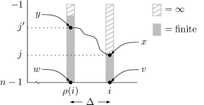
Figure 4: Diagram supporting the proof of Lemma 17.

$$D(x)\,\geqslant\,D(y)+(j-j^{\prime})-\Updelta.$$ (17)

Now assume $\textup{block}(y)>8\Updelta$. We will show that this leads to contradiction. First, observe that

$$D(y)\,\geqslant\,D(w)-\big{(}(n-1)-j^{\prime}\big{)}+(\textup{block}(y)-1)\,\geqslant\,D(w)-n+j^{\prime}+8\Updelta.$$

By Definition 5, $\textup{block}(x)\leqslant 3\Updelta$. By Lemma 16, the start value of a block is at most the end value of the previous block plus one. Thus,

$$D(x)\,\leqslant\,D(v)-\big{(}(n-1)-j\big{)}+2(\textup{block}(x)-1)\,\leqslant\,D(v)-n-1+j+6\Updelta.$$

Plugging the last two inequalities into Inequality (17) gives

$$D(v)-n-1+j+6\Updelta\,\geqslant\,\big{(}D(w)-n+j^{\prime}+8\Updelta\big{)}+(j-j^{\prime})-\Updelta$$

which simplifies to

$$D(v)\,\geqslant\,D(w)+\Updelta+1.$$

To see why this last inequality cannot be true, observe that $D(v)$ is never more than $D(w)+\Updelta$, which is obtained through Equation (10) by using only horizontal edges from $w$ to $v$. ∎

It remains to argue that the running time of Algorithm 2 is $O((\log^{2}n)/w)$ per arriving symbol. In Step 1 of the algorithm, $i-\rho(i)$ symbols of $S$ are read. Each symbol is specified with $\delta=O(\log n)$ bits. In Step 2, up to $8(i-\rho(i))$ blocks are read. Each one can be specified in $O(\log n)$ bits. In Step 3, up to $3(i-\rho(i))$ blocks are written to memory. Thus, when the symbol $S[i]$ arrives, no more than a constant times $(i-\rho(i))\cdot\log n$ bits are read or written. To answer the question of how many bits are read or written over a window of $n$ arriving symbols, starting at any arrival $i^{\prime}$, we first give the following fact.

Lemma 18.

For any $i^{\prime}>0$,

$$\sum_{i=i^{\prime}}^{i^{\prime}+n-1}\big{(}i-\rho(i)\big{)}=O(n\log n).$$

Proof.

Since we sum over $n$ consecutive values we may without loss of generality assume that $i^{\prime}=1$. Let $\alpha(i)$ denote the position of the least significant 1 in the binary representation of $i$. For example, if $i=110100$ (in binary), $\alpha(i)=2$. The sum can be written as

$$\sum_{i=1}^{n}2^{\alpha(i)}\,\leqslant\,\sum_{a=0}^{\log n}\big{(}2^{a}\cdot 2^{(\log n)-a}\big{)}\,=\,O(n\log n).$$

We conclude that over a window of $n$ arriving symbols, a total of $O(n\log n\cdot\log n)$ bits are read or written, hence the algorithm performs $O(n(\log^{2}n)/w)$ cell probes. Amortised over the $n$ arriving symbols, the number of cell probes per arrival is

$$O{\left(\frac{\log^{2}n}{w}\right)}.$$

7.6 Preprocessing the fixed string $F$

Both Algorithms 1 and 2 require that the fixed string $F$ is known so that after Step 1, the relevant part of the DAG can be determined. If $F$ had not been known, the algorithm would have had to probe cells in order to also read in a sufficiently large portion of $F$. Unlike the number $i-\rho(i)$ of symbols being read from $S$, the number of symbols needed from $F$ could potentially span the whole string.

By exploiting the power of the cell-probe model, we may nevertheless design a generic algorithm that takes $F$ as part of the input and has a preprocessing step before the first symbol arrives in the stream. Let

$$\Phi=\{0,\dots,n+1\}^{n+1}.$$

For any $i$, any sequence $D(-1,i),\dots,D(n-1,i)$ corresponds to a unique element $\phi\in\Phi$ such that

$$\phi=\big{(}D(-1,i),\dots,D(n-1,i)\big{)},$$

where $D(j,i)=\infty$ is replaced with the value $n+1$. When $F$ is part of the input, we may precompute all possible values written to memory in Step 3 by considering $F$, every $\phi\in\Phi$ and every string of maximum length $n$ from

$$\Gamma=\bigcup_{k=0}^{n}[2^{\delta}]^{k},$$

where $[2^{\delta}]$ is the alphabet. The precomputed values are inserted into a large dictionary. Thus, after Step 2, the values to write to memory in Step 3 are fetched from the dictionary, where the key is in $\Phi\times\Gamma$ and its value is in $\Phi$. The size of the dictionary is of course infeasibly large, and the preprocessing stage involves an exponential number of cell writes. Nevertheless, there is no additional cost of looking up a key in the dictionary to the cost of probing the cells holding the key and the value associated with it.

The conclusion is that adding a preprocessing step and replacing Step 3 of Algorithm 2 with a dictionary lookup gives us the desired upper bound of Theorem 3.

References

- [1] Raphaël Clifford, Klim Efremenko, Benny Porat and Ely Porat “A Black Box for Online Approximate Pattern Matching” In CPM ’08: Proc. 19th Annual Symp. on Combinatorial Pattern Matching, 2008, pp. 143–151
- [2] Raphaël Clifford, Klim Efremenko, Benny Porat and Ely Porat “A Black Box for Online Approximate Pattern Matching” In Information and Computation 209.4, 2011, pp. 731–736
- [3] Raphaël Clifford and Markus Jalsenius “Lower Bounds for Online Integer Multiplication and Convolution in the Cell-Probe Model” In ICALP ’11: Proc. 38th International Colloquium on Automata, Languages and Programming, 2011, pp. 593–604
- [4] Raphaël Clifford, Markus Jalsenius and Benjamin Sach “Tight Cell-Probe Bounds for Online Hamming Distance Computation” In SODA ’13: Proc. 24th ACM-SIAM Symp. on Discrete Algorithms, 2013, pp. 664–674
- [5] Raphaël Clifford and Benjamin Sach “Online Approximate Matching with Non-local Distances” In CPM ’09: Proc. 20th Annual Symp. on Combinatorial Pattern Matching, 2009, pp. 142–153
- [6] Raphaël Clifford and Benjamin Sach “Pseudo-Realtime Pattern Matching: Closing the Gap” In CPM ’10: Proc. 21st Annual Symp. on Combinatorial Pattern Matching, 2010, pp. 101–111
- [7] M. Fredman “Observations on the complexity of generating Quasi-Gray codes” In SIAM Journal on Computing 7.2, 1978, pp. 134–146
- [8] M. Fredman and M. Saks “The cell probe complexity of dynamic data structures” In STOC ’89: Proc. 21st Annual ACM Symp. Theory of Computing, 1989, pp. 345–354
- [9] Zvi Galil “String Matching in Real Time.” In Journal of the ACM 28.1, 1981, pp. 134–149
- [10] T. Hagerup “Sorting and searching on the word RAM” In STACS ’98: Proc. 15th Annual Symp. on Theoretical Aspects of Computer Science, 1998, pp. 366–398
- [11] Kasper Green Larsen “Higher Cell Probe Lower Bounds for Evaluating Polynomials” In FOCS ’12: Proc. 53rd Annual Symp. Foundations of Computer Science, 2012, pp. 293–301
- [12] Kasper Green Larsen “The cell probe complexity of dynamic range counting” In STOC ’12: Proc. 44th Annual ACM Symp. Theory of Computing, 2012, pp. 85–94
- [13] Peter Bro Miltersen “The Bit Probe Complexity Measure Revisited” In STACS ’93: Proc. 15th Annual Symp. on Theoretical Aspects of Computer Science Springer-Verlag, 1993, pp. 662–671
- [14] M. Minsky and S. Papert “Perceptrons: An Introduction to Computational Geometry” MIT Press, 1969
- [15] M. Pǎtraşcu “Lower bound techniques for data structures”, 2008
- [16] Mihai Pǎtraşcu and Corina Tarniţǎ “On Dynamic Bit-Probe Complexity” See also ICALP’05 In TCS 380, 2007, pp. 127–142
- [17] M. Pătraşcu and E. D. Demaine “Logarithmic Lower Bounds in the Cell-Probe Model” In SIAM Journal on Computing 35.4, 2006, pp. 932–963
- [18] A. C.-C. Yao “Probabilistic computations: Toward a unified measure of complexity” In FOCS ’77: Proc. 18th Annual Symp. Foundations of Computer Science, 1977, pp. 222–227
- [19] Andrew Chi-Chih Yao “Should Tables Be Sorted?” In Journal of the ACM 28.3, 1981, pp. 615–628