Nonreciprocal wave scattering on nonlinear string-coupled oscillators

Abstract

We study scattering of a periodic wave in a string on two lumped oscillators attached to it. The equations can be represented as a driven (by the incident wave) dissipative (due to radiation losses) system of delay differential equations of neutral type. Nonlinearity of oscillators makes the scattering non-reciprocal: the same wave is transmitted differently in two directions. Periodic regimes of scattering are analyzed approximately, using amplitude equation approach. We show that this setup can act as a nonreciprocal modulator via Hopf bifurcations of the steady solutions. Numerical simulations of the full system reveal nontrivial regimes of quasiperiodic and chaotic scattering. Moreover, a regime of a “chaotic diode”, where transmission is periodic in one direction and chaotic in the opposite one, is reported.

One of the mostly general results of the linear wave theory is the reciprocity theorem, established in works of Rayleigh, Helmholtz and Lorentz. For the one-dimensional wave scattering it means the symmetry of the scattering matrix, so that transmission in both direction is the same. While in linear systems violations of reciprocity require violations of time-reversal symmetry, in nonlinear wave propagation reciprocity does not hold. In particular, scattering of linear waves on nonlinear objects may operate as a “wave diode”, with different transmission properties in both directions. Here we consider a simple model of scattering of linear waves on two lumped nonlinear oscillators. If one neglects dispersion and dissipation in the medium and in the oscillators, the equations can be reduced to a system of delay-differential equations. We demonstrate in this paper different regimes of reciprocity violations. In the simplest case transmissions in both directions are different, while the waves remain periodic. We observe also more complex regimes, where reflected and transmitted waves are chaotic and different. Probably, mostly nontrivial regime reported is that of “chaotic diode”: a periodic wave sent to the scatterer in one direction remains periodic, while when the same wave is sent in another direction, transmitted and reflected waves are chaotic.

I Introduction

Understanding the way in which nonlinearity affects wave propagation is one of the basic issues in many different domains such as nonlinear optics, acoustics, electronics and fluid dynamics. A related challenging goal is the control of wave energy flow using fully nonlinear features.

The most elementary form of control would be to devise a “wave diode” in which some input energy is transmitted differently along two opposite propagation directions. As it is known, this is forbidden in a linear, time-reversal symmetric system, by virtue of the reciprocity theorem Rayleigh (1945). The standard way to circumvent this limit is to break the time-reversal symmetry by applying a magnetic field, as done, for instance, in the case of optical isolators. An entirely alternative possibility is instead to consider nonlinear effects. At least in principle, this option would offer novel possibilities of propagation control based on intrinsic material properties rather than on an external field. A general critical discussion of those issues can be found in Ref. Maznev et al., 2013.

The idea of exploiting nonlinear effects has been pursued in different contexts. In the domain of lattice dynamics, asymmetric phonon transmission through a nonlinear layer between two very dissimilar crystals has been demonstrated in Ref. Kosevich, 1995. Other concrete examples are offered by nonlinear phononic media Liang et al. (2009, 2010) and the propagation of acoustic pulses through granular systems Nesterenko et al. (2005); Boechler et al. (2011). Nonlinear optics is also a versatile playground as exemplified by the so-called all-optical diode Scalora et al. (1994); Tocci et al. (1995); Gallo et al. (2001). In particular, in Ref. Maes et al., 2006 symmetry-breaking in two nonlinear microcavities has been described. Other proposals include left-handed metamaterials Feise et al. (2005), quasiperiodic systems Biancalana (2008), coupled nonlinear cavities Grigoriev and Biancalana (2011) or $\mathcal{PT-}$symmetric waveguides Ramezani et al. (2010); D’Ambroise et al. (2012); Bender et al. (2013) and transmission lines Tao et al. (2012). Extensions to the quantum systems Roy (2010); Mascarenhas et al. (2014) and nonlinear Aharanov-Bohm rings Li et al. (2014) have been also considered.

Despite the variety of physical contexts, the basic underlying rectification mechanisms rely on nonlinear phenomena as, for instance, second-harmonic generation in photonic Konotop and Kuzmiak (2002) or phononic crystals Liang et al. (2009), or bifurcations Boechler et al. (2011). In those examples the rectification depends on whether some harmonic (or subharmonic) of the fundamental wave is transmitted or not. As discussed in Ref. Maznev et al., 2013 a more strict operating condition would be that the transmitted power at the same frequency and incident amplitude would be sensibly different in the two opposite propagation directions. Nonlinear resonances have been proved to be effective in achieving this Lepri and Casati (2011) (see also Ref. Xu and Miroshnichenko, 2014 where Fano resonances have been considered).

The above issues are conveniently studied as a scattering problem i.e. by seeking for wave solutions impinging on a nonlinear impurity. In a one-dimensional geometry such solutions can be found by simple methods like the transfer-matrix approach (see Lepri and Casati (2011) and references therein). Once the solutions are known one natural question is the assessment of their dynamical stability and bifurcations. This question has been investigated only to a limited extent Malomed and Azbel (1993); Miroshnichenko (2009). More recently, it has been shown that scattering states in the presence of (generally complex) impurities typically display oscillatory instabilities D’Ambroise et al. (2013) that may results in the creation of stable quasiperiodic, nonreciprocal solutions Lepri and Casati (2014). Those can be seen as a superposition of an extended wave with a nonlinear defect mode oscillating at a different frequency. It can be envisaged that more complex dynamical regimes may be observed and that this will affect the overall performance of any device that one may wish to realize in practice.

In the present paper we introduce a simple model for a scalar wave field interacting with two different local nonlinear elements. It is a generalization of the system introduced in Ref. Pikovsky, 1993 as a simple example of chaotic wave scattering, where only one local nonlinear oscillator coupled to a wave medium was considered. Clearly, with one lumped oscillator the scattering is fully reciprocal, although non-trivial. The model we consider belongs to a class of wave systems with local nonlinearity. In the case of dispersive waves (e.g. in a lattice Brazhnyi and Malomed (2011, 2014) or with a periodic background potential Dror and Malomed (2011)) such a system can possess localized solutions (breathers); a similar situation occurs in a Schrödinger equation with local nonlinearity that creates local pseudopotential well where wave is localized Mayteevarunyoo et al. (2008). We consider here non-dispersive waves, this system does not possess localized solutions.

As it will be shown in Section II, our model can be reformulated as a delay-differential equations and thus admits a very rich dynamics depending of the relation between its relevant time scales. Indeed, complex input-output responses can be easily achieved, including quasiperiodic and chaotic ones. In Section III we start the analysis of the system by considering the case of weak coupling between the string and the oscillators. This limiting case can be treated by means of approximate amplitude equations. In Section IV we turn to the more general case in which there is no sharp separation among timescales and the system can only be treated by direct numerical integration of the full set of equation. Here the dynamics is considerably more complex, leading to high-dimensional and possibly chaotic motion.

II Basic equations

The model is inspired by Ref. Pikovsky, 1993 and is schematically depicted in Fig. 1. It amounts to two lumped, undamped oscillators $v(t)$ and $u(t)$ attached to an elastic string at points $-L/2$ and $L/2$ correspondingly. The equations of motion for the oscillators are

$$m_{1}\ddot{v}+V(v)=S\left(\frac{\partial y^{0}}{\partial x}-\frac{\partial y^{-}}{\partial x}\right)_{x=-L/2}$$ (1)

$$m_{2}\ddot{u}+U(u)=S\left(\frac{\partial y^{+}}{\partial x}-\frac{\partial y^{0}}{\partial x}\right)_{x=L/2}$$ (2)

Here $y^{-}(t,x)$, $y^{0}(t,x)$, and $y^{+}(t,x)$ denote the string displacement in the domains $[-\infty,-L/2)$, $(-L/2,L/2)$ and $(L/2,\infty]$ respectively; $U$ and $V$ are the local forces acting on the two oscillator that we assume to be different to break the mirror symmetry of the system around $x=0$. The string obeys the equation of motion

$$\frac{\partial^{2}y}{\partial t^{2}}-c^{2}\frac{\partial^{2}y}{\partial x^{2}}=0\;,\qquad c^{2}=\frac{S}{\rho}\;,$$

where $S$ is the tension and $\rho$ is the mass density. The energy density of the wave is

$$\mathcal{E}=\frac{1}{2}S\left(\frac{\partial y}{\partial x}\right)^{2}+\frac{1}{2}\rho\left(\frac{\partial y}{\partial t}\right)^{2}$$

and the energy conservation reads

$$\frac{\partial}{\partial t}\mathcal{E}+\frac{\partial}{\partial x}J=0$$ (3)

$$J=-S\frac{\partial y}{\partial x}\frac{\partial y}{\partial t}$$ (4)

with $J$ being the energy flux. We represent the string field as

$$\text{Incident wave: }F(t-(x+L/2)/c)\text{ for }x<-L/2$$

$$\text{reflected wave: }\alpha(x/c+t)\text{ for }x<-L/2$$

$$\text{transmitted wave: }\beta(t-x/c)\text{ for }x>L/2$$

$$\text{``interaction'' waves }\phi(t-x/c),\;\psi(t+x/c)$$

$$\text{ for }-L/2<x<L/2$$

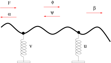
Figure 1: The model.

In the Appendix we show that the problem can be reduced to a coupled system of delay-differential equations for the variables describing the two oscillators. The possibility of such a reduction heavily relies on the non-dispersive, non-dissipative nature of wave propagation along the string. In the case of dispersion and dissipation, one would obtain integro-differential equations that are very hard to investigate.

For convenience, we introduce the time scale according to some frequency $\Omega$, so that the new dimensionless time will be $\tau=\Omega t$. In terms of the dimensionless time delay $T=\Omega L/2c$ and dimensionless coupling parameter $a=\frac{S}{mc\Omega}$, the system of equations reads

$$\frac{d^{2}v}{d\tau^{2}}+2a\frac{dv}{d\tau}+\frac{V(v)}{m\Omega^{2}}=2a\dot{F}(\Omega^{-1}\tau)+2a\dot{\psi}(\tau-T)$$ (5)

$$\frac{d^{2}u}{d\tau^{2}}+2a\frac{du}{d\tau}+\frac{U(u)}{m\Omega^{2}}=2a\dot{\phi}(\tau-T))$$ (6)

$$\dot{\psi}(\tau)=\dot{u}(\tau-T)-\dot{\phi}(\tau-2T)$$ (7)

$$\dot{\phi}(\tau)=\dot{v}(\tau-T)-\dot{\psi}(\tau-2T)$$ (8)

From the system solution we can compute reflected and transmitted waves as

$$\alpha(t-L/2c)=v(t)-F(t);\qquad\beta(t-L/2c)=u(t).$$ (9)

Moreover, one can evaluate the reflected and transmitted fluxes as

$$J_{refl}=-\sqrt{S\rho}\,\dot{\alpha}^{2};\qquad J_{trans}=\sqrt{S\rho}\,\dot{\beta}^{2}.$$ (10)

It should be remarked that the system (5-8) differs from standard delayed dynamical systems (like Ikeda, Mackey-Glass etc.) in several respects. Indeed, one typically has only terms delayed by $T$ while here we have also a reflected components delayed by $2T$. Moreover, and more importantly, the delayed coupling occurs via the derivatives of the variables. This is referred to as “neutral type” of delay-differential equation Hale and Lunel (1993); Bainov and Mishev (1991). Such equations also naturally appear in electrical networks, where lumped elements are connected with lossless transmission lines Miranker (1961); Brayton (1968) that, in fact, is the setup equivalent to the mechanical one of Fig. 1.

Noteworthy, the system (5-8) is dissipative. This is the radiation losses, as the only sink of energy is due to reflected and transmitted waves. The dissipation parameter is the coupling parameter $a$.

III Amplitude equations and their analysis

Let us consider Eqs.(5-8) and set units such that $\Omega=m=c=1$. Furthermore, we specialize to the case of a periodic wave forcing $F(t)=Fe^{i\omega t}+c.c.$. The dynamics is thus characterized by three main timescales, $T$, $1/a$, $1/\omega$. In this Section we first focus on the case of weak coupling whereby $1/a$ is much larger than both $T$ and $1/\omega$. For definiteness, we consider forces of the form

$$U(u)=\omega_{1}^{2}u+k_{1}u^{3}\;,\quad V(v)=\omega_{2}^{2}v+k_{2}v^{3}\;,$$ (11)

and distinguish three distinct regimes where the system equations can be simplified by suitable approximations.

III.1 1:1 resonance

Let us first consider the case in which $\omega\sim\omega_{1}\sim\omega_{2}$. We look for an expansion in slowly varying amplitudes (assuming weak dissipation $a$):

$$v(t)=Ae^{i\omega t}+c.c. \quad\dot{v}(t)=i\omega Ae^{i\omega t}+c.c.$$

$$u(t)=Be^{i\omega t}+c.c. \quad\dot{u}(t)=i\omega Be^{i\omega t}+c.c.$$

$$\phi(t)=\Phi e^{i\omega t}+c.c. \quad\dot{\phi}(t)=i\omega\Phi e^{i\omega t}+c.c.$$

$$\psi(t)=\Psi e^{i\omega t}+c.c. \quad\dot{\psi}(t)=i\omega\Psi e^{i\omega t}+c.c.$$

In the same approximation the transmitted intensity is proportional to $|B|^{2}$. Making use of the rotating wave approximation, we neglect higher-order harmonics i.e.

$$v^{3}\approx 3|A|^{2}Ae^{i\omega t}+c.c.;\quad u^{3}\approx 3|B|^{2}Be^{i\omega t}+c.c.$$

Equating terms proportional to $\sim e^{i\omega t}$ and keeping the lowest order in $a$ in the second-order derivatives we obtain

$$i\dot{A}+(\Delta_{1}+ia+\gamma_{1}|A|^{2})A=ia\left(F+\Psi(t-T)e^{-i\omega T}\right)$$

$$i\dot{B}+(\Delta_{2}+ia+\gamma_{2}|B|^{2})B=ia\Phi(t-T)e^{-i\omega T}$$

$$\Psi(t)=B(t-T)e^{-i\omega T}-\Phi(t-2T)e^{-2i\omega T}$$ (12)

$$\Phi(t)=A(t-T)e^{-i\omega T}-\Psi(t-2T)e^{-2i\omega T}$$

where we have defined the detunings

$$\Delta_{1}=\frac{\omega_{1}^{2}-\omega^{2}}{2\omega}\approx\omega_{1}-\omega;\quad\Delta_{2}=\frac{\omega_{2}^{2}-\omega^{2}}{2\omega}\approx\omega_{2}-\omega$$

and the new nonlinearity parameters $\gamma_{1,2}=3k_{1,2}/2\omega$.

The steady state solutions are thus given by the system of transcendental equations

$$(\Delta_{1}+ia+\gamma_{1}|A|^{2})A=ia\left(F+\Psi e^{-i\omega T}\right)$$ (13)

$$(\Delta_{2}+ia+\gamma_{2}|B|^{2})B=ia\Phi e^{-i\omega T}$$

$$\Psi=Be^{-i\omega T}-\Phi e^{-2i\omega T}$$

$$\Phi=Ae^{-i\omega T}-\Psi e^{-2i\omega T}$$

Solving the last two equations and substituting in the first two yields

$$\Psi=\frac{-Ae^{-i\omega T}+Be^{i\omega T}}{e^{2i\omega T}-e^{-2i\omega T}}$$

$$\Phi=\frac{Ae^{i\omega T}-Be^{-i\omega T}}{e^{2i\omega T}-e^{-2i\omega T}}$$

$$(\Delta_{1}+ia+\gamma_{1}|A|^{2})A=$$

$$=ia\left(F+\frac{-Ae^{-i\omega T}+Be^{i\omega T}}{e^{2i\omega T}-e^{-2i\omega T}}e^{-i\omega T}\right)$$

$$(\Delta_{2}+ia+\gamma_{2}|B|^{2})B=ia\frac{Ae^{i\omega T}-Be^{-i\omega T}}{e^{2i\omega T}-e^{-2i\omega T}}e^{-i\omega T}$$

Note that this solution runs into troubles when $e^{-2i\omega T}=1$, since then the system is undetermined (a “small denominator” problem). Using terminology from optics, this corresponds to the Fabry-Perot resonances $\omega_{n}=\frac{\pi n}{2T}$, $n$ integer, of the modes of the “cavity” represented by the portion of the string comprised between the oscillators.

Away from such resonances equations are solved by introducing the amplitudes and phase shifts as $A=|A|e^{i\theta}$, $B=|B|e^{i(\theta+\rho)}$. Eliminating $\theta$ and $\rho$ we obtain

$$\left[C|A|^{2}-D|B|^{2}\right]^{2}+\frac{a^{2}}{4}\left[|A|^{2}+|B|^{2}\right]^{2}=a^{2}|A|^{2}F^{2}$$

$$\left[D^{2}+\frac{a^{2}}{4}\right]|B|^{2}=\frac{a^{2}}{4}\frac{|A|^{2}}{\sin^{2}2\omega T}$$ (14)

where

$$C\equiv\Delta_{1}+\gamma_{1}|A|^{2}+\frac{a}{2}\cot 2\omega T$$

$$D\equiv\Delta_{2}+\gamma_{2}|B|^{2}+\frac{a}{2}\cot 2\omega T$$

In the symmetric case (i.e. when the oscillators are equal) $\Delta_{1}=\Delta_{2}=\Delta$, $\gamma_{1}=\gamma_{2}=\gamma$, perfectly transmitted solutions $|A|=|B|=F$ exist for $C=D=\pm\frac{a}{2}\cot 2\omega T$ i.e. for

$$\Delta+\gamma F^{2}=0;\quad\Delta+\gamma F^{2}=a\,\cot 2\omega T\quad.$$

The last equations determine the nonlinear resonances of the system: whenever such solutions exist, a multistable regime is expected where asymmetric propagation should set in Lepri and Casati (2011) . This is confirmed in Fig.2 where we plot $|B|^{2}$ versus $F^{2}$ in the bistable regime and compare the symmetric case with two ones in which $\Delta_{1}\neq\Delta_{2}$. The forward (resp. backward) case corresponds to an input applied to the first (resp. second) oscillator. This is obviously equivalent to compare solutions of (13) whereby the two oscillator are exchanged. As it is seen, there are regions close to the nonlinear resonance in which the same input can be transmitted very differently Lepri and Casati (2011). In the case of the lower panel of Fig.2, transmission in one direction is actually almost suppressed.

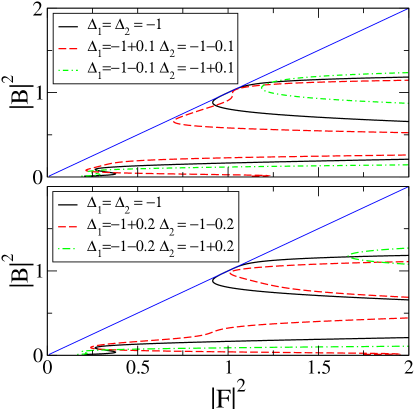
Figure 2: Input-output curves computed from Eq. (14) for $a^{2}=0.4$, $\gamma_{1}=\gamma_{2}=1$, $\omega T=\pi/4$ and different detuning values. In both panels the solid black line corresponds to the symmetric case $\Delta_{1,2}=1$ while dashed and dot-dashed lines are respectively for and $\Delta_{1,2}=-1(1\pm 0.1)$ (upper panel) and $\Delta_{1,2}=-1(1\pm 0.2)$ (lower panel) i.e. the left-to-right and right-to-left transmission for unequal oscillators. The thin solid line is the bisectrix. Note that in the second case for $F\approx 1$ there is basically no transmission in one of the two directions.

To conclude this Subsection, we comment on the dynamics close to the Fabry-Perot resonances. To this aim we let $\omega=\omega_{n}+\epsilon$ with $\epsilon$ being a smallness parameter such that $e^{\pm 2i\omega T}\approx 1\pm 2i\epsilon$ and assume a perturbative expansion

$$A=A_{1}\epsilon+A_{2}\epsilon^{2}\ldots;\quad B=B_{1}\epsilon+B_{2}\epsilon^{2}\ldots;\quad F=F_{1}\epsilon$$

(the last is just a rescaling of the force). Substituting and equating the leading order terms

$$O(1): \quad A_{1}=B_{1}$$

$$O(\epsilon): (\Delta_{1}+ia)A_{1}=iaF_{1}+\frac{a}{4}(-A_{2}+B_{2});$$

$$(\Delta_{2}+ia)A_{1}=\frac{a}{4}(A_{2}-B_{2})$$

From which we find the solution up to corrections $O(\epsilon)$:

$$A=B=\frac{iaF}{\Delta_{1}+\Delta_{2}+2ia};\quad\frac{|B|^{2}}{|F|^{2}}=\frac{a^{2}}{(\Delta_{1}+\Delta_{2})^{2}+4a^{2}}$$

Note that in this limit the nonlinear terms are irrelevant and transmission coefficient is therefore symmetric with respect to the exchange of the two oscillators. So we do not expect sizable reciprocity violations close to resonances.

III.2 Higher-order resonances

As mentioned in the Introduction, we are mostly interested in the case of a transmitted wave having mostly the same frequency as the input one. For completeness, we briefly touch on the problem of higher-order resonances which can be studied with a similar approach. Let us consider for instance the case of a 1:3 resonance, namely the one in which $\omega\sim\omega_{1}\sim\omega_{2}/3$. Conceptually, this corresponds to experimentally relevant situations in which the rectification is induced by excitation of higher-order harmonics Liang et al. (2009); Tao et al. (2012).

The mechanism at work here is the following: the incident wave weakly excites the third harmonic of the first oscillator. The latter is in resonance with the second and can be transmitted. On the other hand, excitation of the second oscillator is negligible since almost no power can be transferred. This suggests looking for solutions of the form

$$v(t)=Ae^{i\omega t}+aA_{3}e^{3i\omega t}+c.c.\quad \dot{v}(t)=i\omega Ae^{i\omega t}+c.c.$$

$$u(t)=aBe^{3i\omega t}+c.c. \dot{u}(t)=3ia\omega Be^{3i\omega t}+c.c.$$

with $\phi$ and $\psi$ having the same form as in previous Subsection. The coupling between oscillators should thus occur through the third-harmonic amplitude $A_{3}$. This means that the asymmetry of transmission should be pretty weak, of order $a^{2}$, and thus not very effective.

III.3 Small delay limit

Consider the case in which $a\ll\omega\sim 1/T$ but $\omega T\to const$. In this limit we can neglect the delay in the Eqs. (III.1) (up to terms of order $O(a^{2})$). It means that the retardation effects enter only through phase shifts. Expressing $\Psi$, $\Phi$ as a function of $A,B$ in the last two Eqs. (III.1), we get

$$i\dot{A}+(\delta_{1}+\frac{ia}{2}+\gamma_{1}|A|^{2})A=iaF+\kappa B$$

$$i\dot{B}+(\delta_{2}+\frac{ia}{2}+\gamma_{2}|B|^{2})B=\kappa A$$ (15)

where we have introduced the new detunings and coupling

$$\delta_{1,2}\equiv\Delta_{1,2}+\frac{a}{2}\cot 2\omega T;\quad\kappa\equiv\frac{a}{2\sin 2\omega T}.$$ (16)

Before proceeding further we note that these equations resemble the ones obtained in Ref. Bulgakov and Sadreev, 2010 for a photonic Fabry-Perot resonator coupled with two off-channel defects.

We performed some numerical experiments with these simplified equations (in rescaled units in which $a=1$ was set).The generic findings are:

1. For a given external input $F$, the dynamics approaches a fixed point or a limit cycle, neither quasiperiodicity nor chaos is observed.

2. The nonreciprocal behavior manifests itself in all the possible combinations of constant output in both directions or constant in one direction and periodic in the other. As this would correspond to a modulation of output in the original model, we may term this as a nonreciprocal modulator.

3. The underlying Hopf bifurcations are typically subcritical when the nonlinearities have the same sign and supercritical otherwise.

The results are exemplified in Figs. 3 and 4. For instance, panels Figs. 4(a) and (c) display a case of a nonreciprocal modulation. Indeed, the output in the forward direction is modulated periodically for amplitudes larger than $F=2.5$ where a subcritical Hopf bifurcation sets in. On the contrary, the output in the backward direction remains periodic in the same ranges of input amplitudes.

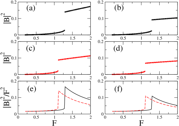
Figure 3: Simulations of Eqs. (15): input-output curves (a-d) and transmission coefficients (e,f) for $\Delta_{1,2}=-2.5(1\pm 0.05)$ and $\omega T=0.5$. Left panels: $\gamma_{1}=\gamma_{2}=1$ right panels $\gamma_{1}=-\gamma_{2}=1$. Panels (a,b) and solid black lines in panels (d,f) refers to the forward propagation; (c,d) and dashed red lines in (d,f) to the backward one; input amplitude $F$ is increased in steps from the lowest value.

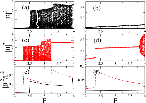
Figure 4: Simulations of Eqs. (15): same as in previous figure with $\omega T=1.4$. For the oscillating amplitude regimes, in panels (e,f) the time-averaged amplitudes are reported.

IV General case

Here we discuss the case where no separation of time scales occurs and we have to integrate the full system Fig. 1 numerically. We report on the results of numerical simulations of (5-8) for $T=8$. The potentials of the two point oscillators are taken in form (11). The system has many parameters, main of them are the eigenfrequencies of the oscillators. In most of the numerical results below we use $\omega_{1}=1.2$, $\omega_{2}=1$, and $k_{1}=k_{2}=1$.

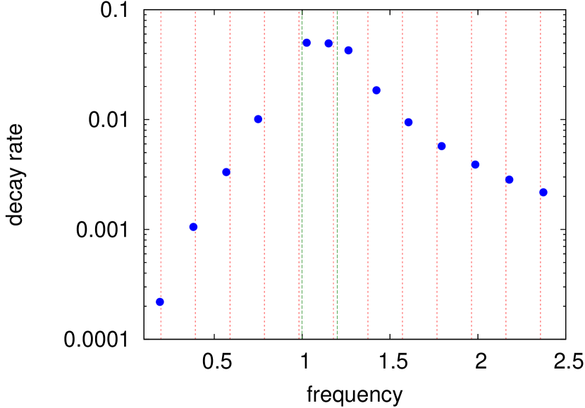
Figure 5: Eigenmodes (blue filled circles) for $\omega_{1}=1$, $\omega_{2}=1.2$ and $a=0.25$. Red dotted lines show Fabry-Perot resonances $\omega_{k}=k\pi/(2T)$, green dashed lines show the oscillator frequencies $\omega_{1,2}$.

To get some insight on the dynamics we first analyze the system (5-8,11) linearized around the trivial fixed point. We report on resulting eigenvalue spectrum in Fig. 5. One can see that while eigenmodes (the Fabry-Perot modes) with frequencies close to that of the oscillators have large decay rates, those with small and large frequencies have very low decay rates. This is a well-known property of hyperbolic systems, and correspondingly of delay systems of neutral type like (5-8). Large (in fact, infinite) number of nearly neutral modes makes many methods of numerical analysis hardly applicable. To avoid excitation of such high-frequency modes, we nearly adiabatically switched on the external field in the study of scattering of the wave on the oscillators.

The main parameters that we change in the study of wave propagation, are the frequency $\omega$ and the amplitude $A$ of the incoming wave, as we choose in (5) $\dot{F}=\omega A\cos(\omega\tau)$. For each amplitude, we focus on violations of reciprocity. Given initially an empty system, we send a wave with the amplitude slowly growing from zero to the maximal value, after which this amplitude remains constant. After transients, we calculate the average transmitted and reflected power; furthermore, correlation properties of the transmitted and reflected waves have been analyzed.

As one can expect, for small amplitudes of the incoming wave the system is fully reciprocal, and we illustrate first deviations from this in Fig. 6(a) where the results for a relatively small amplitude $A=0.2$ are shown. Here nonlinear effects are maximal in the range of frequencies close to that of oscillators, while outside of the range $0.9\lesssim\omega\lesssim 1.3$ the transmission rates in both directions follow the structure of linear modes. Non-reciprocity is much stronger expressed at a larger amplitude $A=1$ (panel (b)). Moreover, here the complexity of the field is rather different for the two ways of propagation. We illustrate this in fig. 7, where we show transmitted waves for $A=1$ and $\omega=1.2467$. While the wave transmitted in one direction is periodic, the wave transmitted in the other direction has a more complex form. Detailed analysis of the autocorrelation function shows however, that the correlations do not decay but the whole process appears quasiperiodic (at the level of our numerical accuracy we cannot in fact distinguish quasiperiodic regimes from periodic ones with large period).

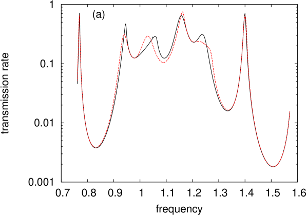
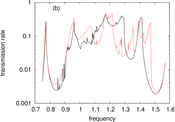
Figure 6: Transmission coefficients in dependence on the frequency of the incoming wave, for $a=0.1$ and two amplitudes: (a) $A=0.2$ and (b) $A=1$. Solid black line: left-to-right, dashed red line: right-to-left.

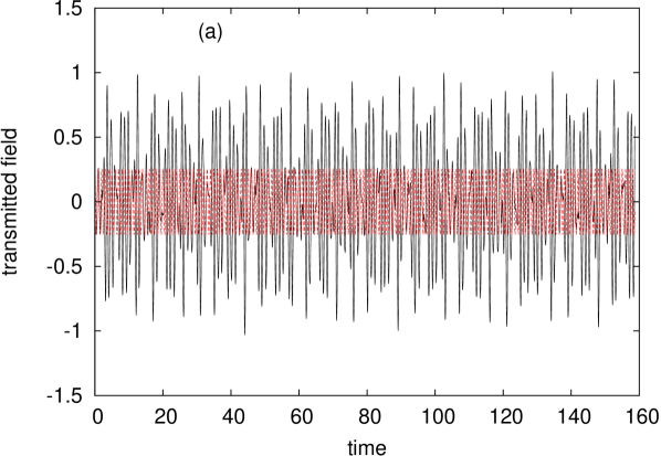
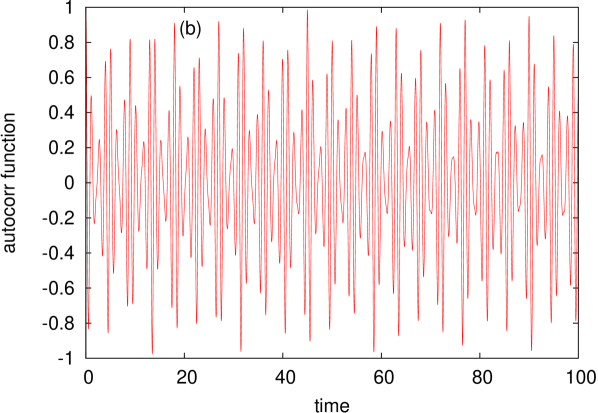
Figure 7: (a) Transmitted waves from left to right (black) and from right to left (red). (b) Autocorrelation function of the black field in panel (a). Time axis is in units of the period of the incident wave.

For large amplitudes of incoming wave chaotic scattering in model (5-8) is observed. We illustrate this in Fig. 8, where we show transmitted fields for $A=20$ and $\omega=1.45$.

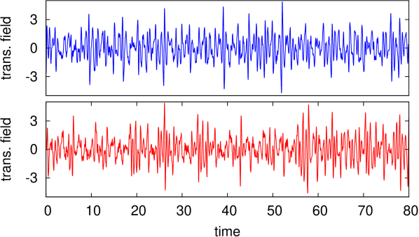
Figure 8: Transmitted waves from left to right (bottom panel) and from right to left (top panel) are chaotic. Time axis is in units of the period of the incident wave.

Probably, the mostly nontrivial situation is when the transmission in one direction is chaotic, while in other direction periodic. We explored several sets of parameters and found such a situation for the “resonant” frequencies of lumped oscillators $\omega_{2}=1.8$, $\omega_{1}=0.6$. This “chaotic diode” regime is illustrated in Fig. 9.

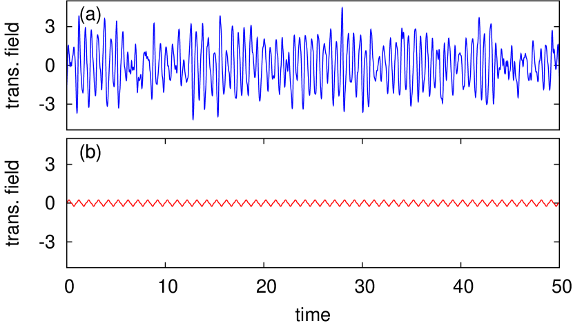
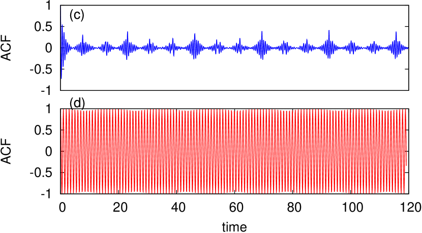
Figure 9: Transmitted waves from left to right ((a), blue) and from right to left ((b), red), and their autocorrelation functions (panels (c,d)). Parameters: $A=16$, $\omega_{1}=0.6$, $\omega_{2}=1.8$, $\omega=1.5$. Time axis is in units of the period of the incident wave.

V Conclusions

In this paper we described non-reciprocity effects in wave scattering on lumped nonlinear oscillators. We have analyzed equations describing a simple model of a linear string with two attached oscillators, on two levels. Close to resonance we used amplitude equations, which allowed us a simplified analysis of transmitted and reflected waves. Here we demonstrated non reciprocity and multistability of scattering. Already at his level of approximation, we have shown that this setup can act as a nonreciprocal modulator via a Hopf bifurcation of the steady solutions.

In the second part, we performed a numerical analysis of full equations, and found more complex regimes of scattering: quasiperiodic and chaotic. A quite interesting finding is that of chaotic non-reciprocity: while a periodic wave sent from one side remains periodic, the same wave sent on the system from the other side becomes chaotic. We think that such a regime might find application in chaotic communication. Unfortunately, we cannot link the two approaches. In the first part the equations are derived in the asymptotic limit of large frequency, which is hardly accessible in numerical studies of the full equations performed in part two. This is mainly due to neutral type of the appearing differential-delay equations. Another difference is that in simulating the full equations we are not limited by a weak nonlinearity, and in fact we considered rather large amplitudes to see chaotic regimes.

In most presented cases we reported scattering states obtained by direct numerical simulations. These yield only stable solutions. In several cases we revealed bistability: scanning solutions by slow change of frequency of the incident wave different regimes have been obtained in some frequency ranges depending on whether it was decreased or increased. One cannot exclude higher degrees of multistability, i.e. co-existence of many stable branches, but such an analysis would require much stronger computational efforts.

In the present work, we focused on an idealized system, where the waves are non-dispersive and there is no dissipation, neither in the wave propagation, nor in the lumped oscillators. This allowed us a coinsize formulation in terms of delayed differential equations, although of neutral type. For more realistic applications, e.g. in optical systems, one needs to incorporate effects of dispersion and diffusion/dissipation. We expect, however, that non-trivial regimes of complex non-reciprocity could be found in such systems as well.

Appendix A Derivation of the equations

In this Appendix we derive the equation of motion of the system. We refer to Fig. 1 and the main text for the definition of the various quantities. For the string field, we have four boundary conditions

$$v(t)=F(t)+\alpha(t-L/2c)=$$

$$\phi(t+L/2c)+\psi(t-L/2c)\;,$$

$$u(t)=\beta(t-L/2c)=\phi(t-L/2c)+\psi(t+L/2c)\;,$$

and the expressions for derivatives

$$\frac{\partial y^{0}}{\partial x}=-\frac{1}{c}\dot{\phi}(t-x/c)+\frac{1}{c}\dot{\psi}(t+x/c)\;,$$

$$\frac{\partial y^{-}}{\partial x}=-\frac{1}{c}\dot{F}(t-(x+L/2)/c)+\frac{1}{c}\dot{\alpha}(t+x/c)\;,$$

$$\frac{\partial y^{+}}{\partial x}=-\frac{1}{c}\dot{\beta}(t-x/c)\;.$$

Substituting this in the equations for $v,u$ we get

$$m_{1}\ddot{v}+V(v)=$$

$$=\frac{S}{c}(-\dot{\phi}(t+L/2c)+\dot{\psi}(t-L/2c)+\dot{F}(t)-\dot{\alpha}(t-L/c))\;,$$

$$m_{2}\ddot{u}+U(u)=$$

$$=\frac{S}{c}(-\dot{\beta}(t-L/2c)-\dot{\psi}(t+L/2c)+\dot{\phi}(t-L/2c))\;.$$

From the boundary conditions we can express $\alpha$ and $\beta$:

$$\beta(t-L/2c)=u(t)\;,\qquad\alpha(t-L/2c)=v(t)-F(t)\;.$$

Substitution of this gives

$$m_{1}\ddot{v}+V(v)=$$

$$\frac{S}{c}(-\dot{\phi}(t+L/2c)+\dot{\psi}(t-L/2c)+\dot{F}(t)-\dot{v}(t)+\dot{F}(t))\;,$$

$$m_{2}\ddot{u}+U(u)=\frac{S}{c}(-\dot{u}(t)-\dot{\psi}(t+L/2c)+\dot{\phi}(t-L/2c))\;.$$

Furthermore, substituting

$$\dot{\psi}(t+L/2c)=-\dot{\phi}(t-L/2c)+\dot{u}(t)\;,$$

$$\dot{\phi}(t+L/2c)=-\dot{\psi}(t-L/2c)+\dot{v}(t)\;,$$

yields the final system

$$m_{1}\ddot{v}+V(v)=\frac{S}{c}(2\dot{\psi}(t-L/2c)+2\dot{F}(t)-2\dot{v}(t))\;,$$

$$m_{2}\ddot{u}+U(u)=\frac{S}{c}(-2\dot{u}(t)+2\dot{\phi}(t-L/2c))\;,$$

$$\dot{\psi}(t)=\dot{u}(t-L/2c)-\dot{\phi}(t-2L/2c)\;,$$

$$\dot{\phi}(t)=\dot{v}(t-L/2c)-\dot{\psi}(t-2L/2c)\;.$$

We introduce the time scale according to some frequency $\Omega$, so that the new dimensionless time will be $\tau=\Omega t$. Furthermore, we restrict to the case $m_{1}=m_{2}=m$. Then

$$\frac{d^{2}v}{d\tau^{2}}+\frac{V(v)}{m\Omega^{2}}=\frac{S}{mc\Omega}(2\dot{\psi}(\tau-\Omega L/2c)+2\dot{F}(\Omega^{-1}\tau)-2\dot{v})\;,$$

$$\frac{d^{2}u}{d\tau^{2}}+\frac{U(u)}{m\Omega^{2}}=\frac{S}{mc\Omega}(-2\dot{u}+2\dot{\phi}(\tau-\Omega L/2c))\;,$$

$$\dot{\psi}(\tau)=\dot{u}(\tau-\Omega L/2c)-\dot{\phi}(\tau-2\Omega L/2c)\;,$$

$$\dot{\phi}(\tau)=\dot{v}(\tau-\Omega L/2c)-\dot{\psi}(\tau-2\Omega L/2c)\;.$$

which upon suitable parameter redefinition reduces to system (5)-(8).

References

- Rayleigh (1945) J. Rayleigh, The theory of sound (Dover publications, New York, 1945).
- Maznev et al. (2013) A. A. Maznev, A. G. Every, and O. B. Wright, Wave Motion 50, 776 (2013).
- Kosevich (1995) Y. A. Kosevich, Phys. Rev. B 52, 1017 (1995).
- Liang et al. (2009) B. Liang, B. Yuan, and J. chun Cheng, Phys. Rev. Lett. 103, 104301 (2009).
- Liang et al. (2010) B. Liang, X. Guo, J. Tu, D. Zhang, and J. Cheng, Nature Materials 9, 989 (2010), ISSN 1476-1122.
- Nesterenko et al. (2005) V. F. Nesterenko, C. Daraio, E. B. Herbold, and S. Jin, Phys. Rev. Lett. 95, 158702 (2005).
- Boechler et al. (2011) N. Boechler, G. Theocharis, and C. Daraio, Nature Materials 10, 665 (2011).
- Scalora et al. (1994) M. Scalora, J. P. Dowling, C. M. Bowden, and M. J. Bloemer, J. Appl. Phys. 76, 2023 (1994).
- Tocci et al. (1995) M. D. Tocci, M. J. Bloemer, M. Scalora, J. P. Dowling, and C. M. Bowden, Appl. Phys. Lett. 66, 2324 (1995).
- Gallo et al. (2001) K. Gallo, G. Assanto, K. Parameswaran, and M. Fejer, Appl. Phys. Lett. 79, 314 (2001).
- Maes et al. (2006) B. Maes, M. Soljacic, J. D. Joannopoulos, P. Bienstman, R. Baets, S.-P. Gorza, and M. Haelterman, Opt. Express 14, 10678 (2006).
- Feise et al. (2005) M. W. Feise, I. V. Shadrivov, and Y. S. Kivshar, Phys. Rev. E 71, 037602 (2005).
- Biancalana (2008) F. Biancalana, J. Appl. Phys. 104, 093113 (2008).
- Grigoriev and Biancalana (2011) V. Grigoriev and F. Biancalana, Opt. Lett. 36, 2131 (2011).
- Ramezani et al. (2010) H. Ramezani, T. Kottos, R. El-Ganainy, and D. N. Christodoulides, Phys. Rev. A 82, 043803 (2010).
- D’Ambroise et al. (2012) J. D’Ambroise, P. G. Kevrekidis, and S. Lepri, J. Phys. A: Math. Theor. 45, 444012 (2012).
- Bender et al. (2013) N. Bender, S. Factor, J. Bodyfelt, H. Ramezani, D. Christodoulides, F. Ellis, and T. Kottos, Phys. Rev. Lett. 110, 234101 (2013).
- Tao et al. (2012) F. Tao, W. Chen, J. Pan, W. Xu, and S. Du, Chaos, Solitons & Fractals 45, 810 (2012).
- Roy (2010) D. Roy, Phys. Rev. B 81, 155117 (2010).
- Mascarenhas et al. (2014) E. Mascarenhas, D. Gerace, D. Valente, S. Montangero, A. Auffèves, and M. F. Santos, EPL (Europhysics Letters) 106, 54003 (2014).
- Li et al. (2014) Y. Li, J. Zhou, F. Marchesoni, and B. Li, Scientific reports 4 (2014).
- Konotop and Kuzmiak (2002) V. V. Konotop and V. Kuzmiak, Phys. Rev. B 66, 235208 (2002).
- Lepri and Casati (2011) S. Lepri and G. Casati, Phys. Rev. Lett. 106, 164101 (2011).
- Xu and Miroshnichenko (2014) Y. Xu and A. E. Miroshnichenko, Phys. Rev. B 89, 134306 (2014).
- Malomed and Azbel (1993) B. A. Malomed and M. Y. Azbel, Phys. Rev. B 47, 10402 (1993).
- Miroshnichenko (2009) A. E. Miroshnichenko, Phys. Lett. A 373, 3586 (2009).
- D’Ambroise et al. (2013) J. D’Ambroise, P. G. Kevrekidis, and S. Lepri, Chaos 23, 023109 (2013).
- Lepri and Casati (2014) S. Lepri and G. Casati, in Localized Excitations in Nonlinear Complex Systems (Springer International Publishing, 2014).
- Pikovsky (1993) A. Pikovsky, Chaos 3, 505 (1993).
- Brazhnyi and Malomed (2011) V. A. Brazhnyi and B. A. Malomed, Phys. Rev. A 83, 053844 (2011).
- Brazhnyi and Malomed (2014) V. A. Brazhnyi and B. A. Malomed, Optics Communications 324, 277 (2014).
- Dror and Malomed (2011) N. Dror and B. A. Malomed, Phys. Rev. A 83, 033828 (2011).
- Mayteevarunyoo et al. (2008) T. Mayteevarunyoo, B. A. Malomed, and G. Dong, Phys. Rev. A 78, 053601 (2008).
- Hale and Lunel (1993) J. Hale and S. V. Lunel, Introduction to Functional-Differential Equations, vol. 99 (Springer-Verlag New York, 1993).
- Bainov and Mishev (1991) D. D. Bainov and D. P. Mishev, Oscillation theory for neutral differential equations with delay (IOP Publ. Bristol, 1991).
- Miranker (1961) W. Miranker, IBM Journal of Research and Development 5, 2 (1961).
- Brayton (1968) R. Brayton, IBM Journal of Research and Development 12, 431 (1968).
- Bulgakov and Sadreev (2010) E. N. Bulgakov and A. F. Sadreev, Phys. Rev. B 81, 115128 (2010).