Phonon dynamics in correlated quantum systems driven away from equilibrium

Abstract

A general form of a many-body Hamiltonian is considered, which includes an interacting fermionic sub-system coupled to non-interacting extended fermionic and bosonic systems. We show that the exact dynamics of the extended bosonic system can be derived from the reduced density matrix of the sub-system alone, despite the fact that the latter contains information about the sub-system only. The advantage of the formalism is immediately clear: While the reduced density matrix of the sub-system is readily available, the formalism offers access to observables contained in the full density matrix, which is often difficult to obtain. As an example, we consider an extended Holstein model and study the nonequilibrium dynamics of the, so called, “reaction mode” for different model parameters. The effects of the phonon frequency, the strength of the electron-phonon couplings, and the source-drain bias voltage on the phonon dynamics across the bistability are discussed.

Strongly correlated systems show a remarkable range of interesting phenomena, some of which can be explained with the current arsenal of theoretical tools Saxena and Littlewood (2012); Tsvelik (2001). Their behavior when driven away from equilibrium (e.g., by a finite bias voltage) is less well understood Stefanucci and Leeuwen (2013). This is because theoretical tools that provide a reliable and accurate description under equilibrium conditions are difficult to converge for open quantum systems driven away from equilibrium Schmitteckert (2004); Anders and Schiller (2005). For example, Kondo physics in equilibrium has been understood within renormalization group theory for several decades Wilson (1975), while the spectral properties under bias Wingreen and Meir (1994) were only recently solved exactly by newly developed a numerical real-time quantum Monte Carlo formalism Mühlbacher and Rabani (2008); Gull et al. (2010), confirming the voltage splitting of the Kondo peak Cohen et al. (2014). The lack of a robust theoretical framework to nonequilibrium many-body physics has been the driving force for developing theoretical tools to understand both the dynamics and the approach to steady-state when strong correlations are dominant.

One such powerful tool is based on the Nakjima–Zwanzig reduced density matrix (RDM) formalism Nakajima (1958); Zwanzig (1960, 2001) combined with a proper impurity solver to obtain the memory kernel Cohen and Rabani (2011). This approach has been applied recently to study charge and spin relaxation near the Kondo crossover temperature of the Anderson impurity model Cohen et al. (2013a) and to study localization and bistability in the nonequilibrium extended Holstein model Wilner et al. (2013, 2014). The Nakjima–Zwanzig formalism, by construction, provides access to the dynamics of observables within the reduced space only. Here, we expand the methodology and show how to extract the dynamics of a certain class of observables that were traced out. Our approach is particularly suitable for systems with strong electron-phonon couplings, which give rise to highly interesting phenomena Blum et al. (2005); Sapmaz et al. (2006); Leturcq et al. (2009); Lassange et al. (2009); Secker et al. (2011). In light of this, we apply the formalism to analyze nonequilibrium phonon dynamics in the extended Holstein model. While the nonequilibrium phonon distribution in the steady state of this model has been analyzed in great detail (see e.g. Galperin et al. (2004); Mitra et al. (2004); Koch and von Oppen (2005); Galperin et al. (2007); Volkovich et al. (2011) and references therein), so far there are only very few theoretical studies of time-dependent phonon dynamics, which all involve significant approximations Metelmann and Brandes (2011); Lü et al. (2012); Vinkler et al. (2012); Albrecht et al. (2013). The methodology presented in this paper facilitates a numerically converged treatment of this nonequilibrium many-body problem.

To outline the reduced density matrix formalism, consider a general Hamiltonian for a many-body quantum system comprising bosons and fermions

$$H=H_{s}+H_{f}+H_{b}+V_{sf}+V_{sb},$$ (1)

where $H_{s}=\sum_{ij}\varepsilon_{ij}d_{i}^{\dagger}d_{j}+\sum_{ijnm}V_{ijnm}d_{i}^{\dagger}d_{j}^{\dagger}d_{n}d_{m}$ and $H_{f}=\sum_{kq}\varepsilon_{kq}c_{k}^{\dagger}c_{q}$ are the interacting and non-interacting parts of the Hamiltonian for the fermionic degrees of freedom and $H_{b}=\sum_{\alpha}\hbar\omega_{\alpha}\left(b_{\alpha}^{\dagger}b_{\alpha}+\frac{1}{2}\right)$ describes the bosonic degrees of freedom. The coupling between the sub-space “$s$” and “$f$” is described by $V_{sf}$ and often is chosen in the form of a hopping between sites, $\sum_{ik}\left(t_{ik}d_{i}^{\dagger}c_{k}+h.c.\right)$, but the formalism developed below is not limited to this choice. The coupling between the interacting fermions and bosons is taken to the lowest order in dimensionless boson coordinates, $x_{\alpha}=\frac{1}{\sqrt{2}}\left(b_{\alpha}^{\dagger}+b_{\alpha}\right)$:

$$V_{sb}=\sum_{ij,\alpha}M_{ij}^{\alpha}d_{i}^{\dagger}d_{j}x_{\alpha}.$$ (2)

Here, $d_{i}^{\dagger}$/$d_{i}$ and $c_{k}^{\dagger}/c_{k}$ are fermionic creation/annihilation operators at site $i$ and $k$, respectively, and $b_{\alpha}^{\dagger}$/$b_{\alpha}$ are bosonic creation/annihilation operators for mode $\alpha$. The above many-body Hamiltonian is a general form covering different generic models, e.g., Fermi-Bose Hubbard model Hubbard (1963), the spin-boson model Leggett et al. (1987), and the Anderson-Holstein quantum impurity model Anderson (1961); Holstein (1959). Thus, developing an approach to extract the time-dependent solution of this generic model is of great importance.

Using the projection operator $\mathcal{P}=\rho_{f}\left(0\right)\otimes\rho_{b}\left(0\right)Tr_{f,b}$, where $\rho_{f}\left(0\right)\otimes\rho_{b}\left(0\right)$ is the initial density matrix in the “$b$” and “$f$” sub-spaces and the trace $Tr_{f,b}$ is performed only for these degrees of freedom, one can derive an exact equation of motion for the RDM of sub-space “$s$” (referred to as the “system”) Wilner et al. (2013):

$$i\hbar\frac{\partial}{\partial t}\sigma\left(t\right)=\mathcal{L}_{s}\sigma\left(t\right)+\vartheta\left(t\right)-\frac{i}{\hbar}\int_{0}^{t}d\tau\kappa\left(\tau\right)\sigma\left(t-\tau\right),$$ (3)

where $\sigma\left(t\right)=Tr_{f,b}\,\rho\left(t\right)$ and $\rho\left(t\right)$ is the full time-dependent density matrix obeying the Liouville–Von-Neumann equation $\dot{\rho}=\frac{i}{\hbar}\left[H,\rho\right]$. In the above equation, $\mathcal{L}_{s}=[H_{s},\cdots]$ is the system’s Liouvillian,

$$\vartheta\left(t\right)=Tr_{f,b}\left\{\mathcal{L}_{v}e^{-\frac{i}{\hbar}\mathcal{Q}\mathcal{L}t}\mathcal{Q}\rho\left(0\right)\right\}$$ (4)

is a super-operator matrix, that depends on the choice of initial conditions and $\mathcal{L}_{v}=[V_{sf}+V_{sb},\cdots]$. By construction, $\vartheta\left(t\right)$ vanishes for an uncorrelated initial state Wilner et al. (2013), i.e. when $\rho(0)=\sigma(0)\otimes\rho_{f}\left(0\right)\otimes\rho_{b}\left(0\right)$, where $\sigma(0)$ is the system initial density matrix. The memory kernel super-operator, $\kappa\left(\tau\right),$ which describes the non-Markovian dependency of the time propagation of the system, is given by Wilner et al. (2013)

$$\kappa\left(t\right)=Tr_{f,b}\left\{\mathcal{L}_{v}e^{-\frac{i}{\hbar}\mathcal{Q}\mathcal{L}t}\mathcal{Q}\mathcal{L}\left(\rho_{f}\left(0\right)\otimes\rho_{b}\left(0\right)\right)\right\}$$ (5)

with $\mathcal{Q}=1-\mathcal{P}$.

The calculation of the RDM in Eq.(3) requires as input the knowledge of the time-dependent memory kernel. The difficulty in solving the many-body quantum Liouville–Von-Neumann equation for $\rho\left(t\right)$ is now shifted to obtaining $\kappa\left(t\right)$. However, simplifications can be made and rely on the fact that often the memory kernel is short-lived (the time scale is typically governed by a large energy scale), i.e., the system “forgets” its history rapidly Cohen et al. (2013b). Therefore, one can develop suitable quantum impurity solvers to calculate the memory until it decays and obtain the dynamics of the RDM at all times using Eq. (3).

The Nakjima–Zwanzig formalism, by construction, provides access to the dynamics of observables within the reduced space only. Observables that depend also on non-system degrees of freedom ($\in f,b$) can, in principle, be calculated by introducing additional sets of Nakjima–Zwanzig like equations. For example, for open quantum systems, the current which depends both on $s$ and $f$ operators requires the introduction of an additional memory term with a longer decay time Cohen et al. (2013b). The drawback of this extended Nakjima–Zwanzig formalism for non-system operators is that each observable requires the introduction of an additional memory term, which is often difficult (or perhaps impossible) to calculate.

We propose an alternative formalism suitable for a certain class of observables that does not require any additional calculation of memory terms or the inclusion of the boson degrees of freedom in the system part. More specifically, we show that the time evolution of the expectation values of the positions and momenta of the bosonic variables can be obtained from the RDM (or from the lesser two-time Green function, $G^{<}\left(t,t\right)$) of the system alone, despite the fact that $\sigma\left(t\right)$ (or $G^{<}\left(t,t\right)$) does not contain any information about the bosonic bath that was traced out. The derivation given below is rather simple but the result is powerful. It offers a way to extract information which is not directly accessible. We illustrate the approach for the extended nonequilibrium Holstein model and discuss the correlations between the phonon and electron dynamics.

Consider the Heisenberg equation of motion for $b_{\alpha}\left(t\right)$ and $b_{\alpha}^{\dagger}\left(t\right)$ generated by the general Hamiltonian of Eq. (1):

$$\dot{b}_{\alpha}\left(t\right) = -i\omega_{\alpha}b_{\alpha}\left(t\right)-\frac{i}{\sqrt{2}\hbar}\sum_{ij}M_{ij}^{\alpha}d_{i}^{\dagger}\left(t\right)d_{j}\left(t\right)$$

$$\dot{b}_{\alpha}^{\dagger}\left(t\right) = i\omega_{\alpha}b_{\alpha}^{\dagger}\left(t\right)+\frac{i}{\sqrt{2}\hbar}\sum_{ij}M_{ij}^{\alpha}d_{i}^{\dagger}\left(t\right)d_{j}\left(t\right),$$ (6)

where the dimensionless position and momentum of each boson mode is given by $x_{\alpha}\left(t\right)=\frac{1}{\sqrt{2}}\left(b_{\alpha}^{\dagger}\left(t\right)+b_{\alpha}\left(t\right)\right)$ and $p_{\alpha}\left(t\right)=\frac{i}{\sqrt{2}}\left(b_{\alpha}^{\dagger}\left(t\right)-b_{\alpha}\left(t\right)\right)$, respectively. Taking the expectation value over the initial density matrix, $\rho(0)$, we find that:

$$\left\langle\dot{x}_{\alpha}\left(t\right)\right\rangle = \omega_{\alpha}\left\langle p_{\alpha}\left(t\right)\right\rangle$$ (7)

$$\left\langle\dot{p}_{\alpha}\left(t\right)\right\rangle = -\omega_{\alpha}\left\langle x_{\alpha}\left(t\right)\right\rangle-\frac{1}{\hbar}\sum_{ij}M_{ij}^{\alpha}\left\langle d_{i}^{\dagger}\left(t\right)d_{j}\left(t\right)\right\rangle,$$

where $\left\langle\cdots\right\rangle\equiv Tr[\rho(0)\cdots].$ The expectation value of the site populations and coherences can be expressed in terms of the RDM (for the same sake by the elements of the Green function of the system) by

$$\left\langle d_{i}^{\dagger}d_{i}\right\rangle = \sum_{\begin{array}[t]{c}n_{1},\ldots n_{N}\end{array}}\sigma_{n_{1},\ldots n_{N},n_{1},\ldots n_{N}}\delta_{n_{i},1}$$ (9)

$$\left\langle d_{i}^{\dagger}d_{j}\right\rangle = \sum_{\begin{array}[t]{c}n_{1},\ldots n_{N}\\ n_{1}^{{}^{\prime}},\ldots n_{N}^{{}^{\prime}}\end{array}}\sigma_{n_{1},\ldots n_{N},n_{1},\ldots n_{N}}\delta_{n_{i},1}\delta_{n_{j},0}\delta_{n_{i}^{{}^{\prime}},0}\delta_{n_{j}^{{}^{\prime}},1}$$ (12)

Eqs. (7) and (9) imply that if the RDM of the system is known the average positions and momenta of the boson modes can be obtained by solving for Eq. (7) with the RDM given as an input. This is the main result of this letter. We now illustrate this for the extended Holstein model.

In this model, $H_{s}=\varepsilon d^{\dagger}d$ includes a single level, $H_{f}=\sum_{k\in L,R}\varepsilon_{k}c_{k}^{\dagger}c_{k}$, and $H_{b}=\sum_{\alpha}\hbar\omega_{\alpha}\left(b_{\alpha}^{\dagger}b_{\alpha}+\frac{1}{2}\right)$. The coupling between the system and the fermionic and bosonic baths is given by $V_{sf}=\sum_{k}t_{k}d^{\dagger}c_{k}+h.c.$ and $V_{fb}=d^{\dagger}d\sum_{\alpha}M_{\alpha}\left(b_{\alpha}^{\dagger}+b_{\alpha}\right)$, respectively. $t_{k}$ and $M_{\alpha}$ determine the strength of the hybridization and electron-phonon couplings, respectively. The former is modeled by a tight-binding spectral density with an overall coupling determined by $\Gamma$ while the latter is modeled by an Ohmic spectral density $J\left(\omega\right)=\frac{\pi\hbar}{2}\eta\omega e^{-\frac{\omega}{\omega_{c}}}$, where the dimensionless Kondo parameter, $\eta=\frac{2\lambda}{\hbar\omega_{c}}$, determines the overall electron-phonon couplings, $\omega_{c}$ is the characteristic phonon bath frequency, and $\lambda=\sum_{\alpha}\frac{M_{\alpha}^{2}}{\hbar\omega_{\alpha}}=\frac{1}{\pi}\int\frac{d\omega}{\omega}J(\omega)$ is the reorganization energy (or polaron shift), which also determines the shifting of the dot energy upon charging.

The reduced density matrix was recently solved for this model Wilner et al. (2013, 2014) by employing two different approaches to calculate the memory kernel and solving Eq. (3) for $\sigma\left(t\right)$: (i) a two-time nonequilibrium Green function (NEGF) Myöhänen et al. (2010) method within the self-consistent Born approximation (SCBA) Wilner et al. (2014) suitable for weak electron-phonon couplings and (ii) the multilayer multiconfiguration time-dependent Hartree (ML-MCTDH) Wang and Thoss (2003, 2009), which is numerically exact but more demanding. The results obtained in a wide range of parameters revealed dynamics on multiple timescales. In addition to the short and intermediate timescales associated with the separate electronic and phononic degrees of freedom, the electron-phonon coupling introduces longer timescales related to the adiabatic or nonadiabatic tunneling between the two charge states ($\langle d^{\dagger}d\rangle=1$ and $\langle d^{\dagger}d\rangle=0$). The analysis shows, furthermore, that the value of the dot occupation may depend on the initial preparation of the phonon degrees of freedom, suggesting the existence of bistability Gogolin and Komnik (2002); Galperin et al. (2004); Albrecht et al. (2012); Wilner et al. (2013, 2014). Intriguingly, the phenomenon of bistability persists even on timescales longer than the adiabatic/nonadiabatic tunneling time.

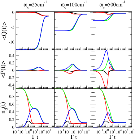
Figure 1: $n_{d}\left(t\right)=\langle d^{\dagger}d\rangle(t),$ $\left\langle P\left(t\right)\right\rangle$, and $\left\langle Q\left(t\right)\right\rangle$ for different initial conditions: Black - unoccupied ($n_{d}\left(0\right)=0$) with $\left\langle x_{\alpha}\left(0\right)\right\rangle=0$, Red - occupied ($n_{d}\left(0\right)=1$) with $\left\langle x_{\alpha}\left(0\right)\right\rangle=0$, Blue - unoccupied with $\left\langle x_{\alpha}\left(0\right)\right\rangle=-\frac{2M_{\alpha}}{\hbar\omega_{\alpha}}$ and Green - occupied with $\left\langle x_{\alpha}\left(0\right)\right\rangle=-\frac{2M_{\alpha}}{\hbar\omega_{\alpha}}$. The model parameters are $\lambda/\Gamma=0.77$, $\varepsilon_{d}/\Gamma=1.5625$, $\Delta\mu/\Gamma=0.625$, and temperature $T=0$.

In Fig. 1 we show the correlation between the dynamics of the average dot occupation, the reaction mode $\left\langle Q\left(t\right)\right\rangle=\sum_{\alpha}M_{\alpha}\left\langle x_{\alpha}\left(t\right)\right\rangle/\sqrt{\sum_{\alpha}M_{\alpha}^{2}}$, and its corresponding momentum, $\left\langle P\left(t\right)\right\rangle=\left\langle\dot{Q}\left(t\right)\right\rangle/\Omega$, where $\Omega=\frac{\int d\omega J\left(\omega\right)}{\int d\omega\frac{J\left(\omega\right)}{\omega}}=\omega_{c}$ is the reaction mode frequency. These results were obtained for weak electron-phonon couplings by solving the memory kernel required to obtain the RDM using the two-time NEGF with in the SCBA. Within this limit, the NEGF–SCBA provides an accurate description of the RDM in comparison to the numerically exact ML-MCTDH-SQR approach Wang and Thoss (2003, 2009). We consider $4$ different initial conditions for the system and boson bath, namely all combinations of initial occupied/unoccupied ($n_{d}\left(0\right)=0/1$) dot and shifted ($\left\langle x_{\alpha}\left(0\right)\right\rangle=-\frac{2M_{\alpha}}{\hbar\omega_{\alpha}}$)/unshifted ($\left\langle x_{\alpha}\left(0\right)\right\rangle=0$) phonon modes. These shifted/unshifted values of $\left\langle x_{\alpha}\left(0\right)\right\rangle$ correspond to the location of the minimum of diabatic potential energy of the occupied/unoccupied dot.

At long times, the dot population (lower panels of Fig. 1) decays to a unique value (closer to the empty state) regardless of the initial preparation of the system and phonon bath, with a typical decay time inversely proportional to $\Omega$ for the shifted bath and to $\Gamma$ for the unshifted bath. The average position $\left\langle Q\left(t\right)\right\rangle$ and its corresponding momentum $\left\langle P\left(t\right)\right\rangle$ follow the population dynamics. At $t=0$, $\left\langle Q(0)\right\rangle$ assumes two different values corresponding to the left/right potential minimum. Regardless of the initial conditions, the motion of the reaction mode is overdamped (i.e. no oscillations are observed). This is known to occur for the reaction mode of a bosonic bath with Ohmic spectral density. At long times, the average position decays to values corresponding to the more stable well, consistent with the behavior of the dot populations. The typical time scale for approaching the steady-state value is given by $\Omega$ (and not by $\Gamma$) regardless of the initial conditions and varies only slightly for an unoccupied initial dot.

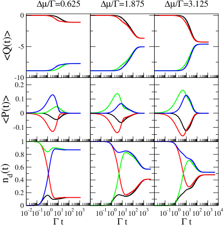
Figure 2: Same as Fig. 1 for different values of the bias voltage. The model parameters are $\lambda/\Gamma=\varepsilon_{d}/\Gamma=1.5625$ and $\omega_{c}=100\mbox{cm${}^{-1}$}$.

The qualitative behavior of the dot population changes when the coupling to the boson bath increases. In Fig. (2) we show the results for a larger value of $\lambda=\varepsilon_{d}$ and different bias voltages $\Delta\mu$, still within the validity of the NEGF-SCBA. In this case, both potential minima are degenerate and the related spin-boson model (at equilibrium) shows a localization transition at temperature $T=0$, which is broadened and finally disappears as $T$ is increased. The appearance of two distinct values of the dot population at long times at small bias voltages ($\Delta\mu$) is consistent with the equilibrium results for the spin-boson model. The bias voltage plays a similar role of temperature, and as its value increases the bistability disappears.

Turning to discuss the transient behavior of $\left\langle Q\left(t\right)\right\rangle$ and $\left\langle P\left(t\right)\right\rangle$, we find that similar to the previous case of weaker electron-phonon couplings, the average position of the reaction coordinate follows closely the transient behavior of the dot population. At long times $\left\langle Q\left(t\right)\right\rangle$ assumes two values roughly corresponding to the two minima of the potential energy along the reaction mode, with vanishing differences as $\Delta\mu$ increases. The corresponding average momenta always decays to zero at long times, regardless of the initial conditions of the dot and boson bath, suggesting that on the time scale observed $\left\langle P\left(t\right)\right\rangle$ decays to its vanishing steady-state value.

The relation between the behavior of $n_{d}(t)$ and $\left\langle Q\left(t\right)\right\rangle$ at steady state can be derived analytically. Since at steady-state $\left\langle\dot{p}_{\alpha}\left(t\right)\right\rangle=0$, one finds from Eq. (7) that each boson mode must satisfy the relation $\left\langle x_{\alpha}\right\rangle=-\frac{M_{\alpha}}{\hbar\omega_{\alpha}}n_{d}$ and thus, the difference in $x_{\alpha}$ between the two different initial distributions of the phonon modes is given by $M_{\alpha}\Delta x_{\alpha}=-\frac{M_{\alpha}^{2}}{\hbar\omega_{\alpha}}\Delta n_{d}$, where $\Delta n_{d}$ is the corresponding difference between the two dot populations at steady-state. Summing both sides over $\alpha$, the reaction mode difference, $\Delta Q=\sum_{\alpha}M_{\alpha}\Delta x_{\alpha}/\sqrt{\sum_{\alpha}M_{\alpha}^{2}}$, must satisfy the relation

$$\Delta Q=-\frac{\lambda}{\sqrt{\sum_{\alpha}M_{\alpha}^{2}}}\Delta n_{d},$$ (13)

where as before $\lambda=\sum_{\alpha}\frac{M_{\alpha}^{2}}{\hbar\omega_{\alpha}}$. This is in agreement with the result obtained in Fig. 2.

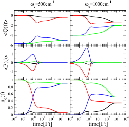
Figure 3: Same as Fig. 1 for $\lambda/\Gamma=3.1$ and $\varepsilon_{d}/\Gamma=3.125$.

So far, we have discussed the appearance of two bistable solutions in the so called adiabatic limit, where $\omega_{c}\ll\Gamma$. In Fig. 3 we show results for larger values of $\omega_{c}$ in the regime where $\omega_{c}\approx\Gamma$. The value of the electron-phonon coupling (reorganization energy) is somewhat larger than the perturbation regime for which the NEGF-SCBA is accurate. Therefore, we obtain the input required to generate the memory kernel and the RDM from the numerically exact ML-MCTDH approach Wang and Thoss (2003, 2009). Similar to the adiabatic limit with weaker electron-phonon couplings (shown in Fig. 2), the long time behavior of $n_{d}\left(t\right)$ depends on the initial conditions of the phonon bath. However, unlike the adiabatic limit, here we find an additional time scale at long times which is associated with the transition from one diabatic potential surface to the other. Intriguingly, however, the bistability prevails at times longer than the tunneling between the two diabatic surfaces. As the phonon frequency increases, the value of $\Delta n_{d}$ decreases and eventually disappears when $\omega_{c}\gg\Gamma$.

Similar to the adiabatic limit, $Q\left(t\right)$ shows the same behavior as $n_{d}\left(t\right)$, including the long time decay associated with the aforementioned tunneling between the diabatic surfaces, and the long time value of $\Delta Q$ is correlated with that of $\Delta n_{d}$, in agreement with Eq. (13). Unlike the transient behavior of the reaction coordinate, its corresponding momentum decays to its steady-state value on a much faster time scale (typically on a time scale given by $\Omega^{-1}$) and does not show the long time relaxation behavior associated with the phonon tunneling. This implies that the tunneling process is not driven by inertia, but is rather in the over-damped limit.

In summary, we have expanded our recently developed nonequilibrium quantum dynamics methodology, which combines reduced density matrix theory with an impurity solver to obtain the memory kernel, to describe phonon dynamics in correlated open quantum systems. Although the phonon degrees of freedom are formally not part of the reduced system, the structure of the equations of motion allows the calculation of phonon observables based solely on the density matrix and memory kernel of the reduced system. The application to a Holstein-type model for phonon-coupled electron transport in nanosystems reveals the intricate interplay between electron and phonon dynamics in these systems, including the phenomenon of bistability.

EYW is grateful to The Center for Nanoscience and Nanotechnology at Tel Aviv University for a doctoral fellowship. HW acknowledges the support from the National Science Foundation CHE-1361150. MT acknowledges support from the German Research Foundation (DFG) and the German-Israeli Foundation for Scientific Research and Development (GIF). This work used resources of the National Energy Research Scientific Computing Center, which is supported by the Office of Science of the U.S. Department of Energy under Contract No. DE-AC02-05CH11231.

References

- Saxena and Littlewood (2012) S. S. Saxena and P. B. Littlewood, J. Phys.: Condens. Matter 24, 290301 (2012).
- Tsvelik (2001) A. Tsvelik, New Theoretical Approaches to Strongly Correlated Systems, NATO science series: Mathematics, physics, and chemistry (Springer Netherlands, 2001).
- Stefanucci and Leeuwen (2013) G. Stefanucci and R. v. Leeuwen, Nonequilibrium Many-Body Theory of Quantum Systems: A Modern Introduction (Cambridge University Press, 2013), ISBN 9780521766173.
- Schmitteckert (2004) P. Schmitteckert, Phys. Rev. B 70, 121302 (2004).
- Anders and Schiller (2005) F. B. Anders and A. Schiller, Phys. Rev. Lett. 95, 196801 (2005).
- Wilson (1975) K. G. Wilson, Rev. Mod. Phys 47, 773 (1975).
- Wingreen and Meir (1994) N. S. Wingreen and Y. Meir, Phys. Rev. B 49, 11040 (1994).
- Mühlbacher and Rabani (2008) L. Mühlbacher and E. Rabani, Phys. Rev. Lett. 100, 176403 (2008).
- Gull et al. (2010) E. Gull, D. R. Reichman, and A. J. Millis, Phys. Rev. B 82, 075109 (2010).
- Cohen et al. (2014) G. Cohen, E. Gull, D. R. Reichman, and A. J. Millis, Phys. Rev. Lett 112, 146802 (2014).
- Nakajima (1958) S. Nakajima, Prog. Theor. Phys. 20, 948 (1958).
- Zwanzig (1960) R. Zwanzig, J. Chem. Phys. 33, 1338 (1960).
- Zwanzig (2001) R. Zwanzig, Nonequilibrium Statistical Mechanics (Oxford University Press, 2001), ISBN 9780195140187.
- Cohen and Rabani (2011) G. Cohen and E. Rabani, Phys. Rev. B 84, 075150 (2011).
- Cohen et al. (2013a) G. Cohen, E. Gull, D. R. Reichman, A. J. Millis, and E. Rabani, Phys. Rev. B 87, 195108 (2013a).
- Wilner et al. (2013) E. Y. Wilner, H. Wang, G. Cohen, M. Thoss, and E. Rabani, Phys. Rev. B 88, 045137 (2013).
- Wilner et al. (2014) E. Y. Wilner, H. Wang, M. Thoss, and E. Rabani, Phys. Rev. B 89, 205129 (2014).
- Blum et al. (2005) A. S. Blum, J. G. Kushmerick, D. P. Long, C. H. Patterson, J. C. Yang, J. C. Henderson, Y. Yao, J. M. Tour, R. Shashidhar, and B. R.Ratna, Nat. Mater. 4, 167 (2005).
- Sapmaz et al. (2006) S. Sapmaz, P. Jarillo-Herrero, Y. M. Blanter, C. Dekker, and H. S. J. van der Zant, Phys. Rev. Lett. 96, 026801 (2006).
- Leturcq et al. (2009) R. Leturcq, C. Stampfer, K. Inderbitzin, L. Durrer, C. Hierold, E. Mariani, M. Schultz, F. von Oppen, and K. Ensslin, Nat. Phys. 5, 327 (2009).
- Lassange et al. (2009) B. Lassange, Y. Tarakanov, J. Kiranet, D. Garcia-Sanchez, and A. Bachthold, Science 325, 1107 (2009).
- Secker et al. (2011) D. Secker, S. Wagner, S. B. R. Härtle, M. Thoss, and H. B. Weber, Phys. Rev. Lett. 106, 136807 (2011).
- Galperin et al. (2004) M. Galperin, M. A. Ratner, and A. Nitzan, J. Chem. Phys. 121, 11965 (2004).
- Mitra et al. (2004) A. Mitra, I. Aleiner, and A. Millis, Phys. Rev. B 69, 245302 (2004).
- Koch and von Oppen (2005) J. Koch and F. von Oppen, Phys. Rev. Lett. 94, 206804 (2005).
- Galperin et al. (2007) M. Galperin, M. A. Ratner, and A. Nitzan, J. Phys.: Condens. Matter 19, 103201 (2007).
- Volkovich et al. (2011) R. Volkovich, R. Härtle, M. Thoss, and U. Peskin, Phys. Chem. Chem. Phys. 13, 14333 (2011).
- Metelmann and Brandes (2011) A. Metelmann and T. Brandes, Phys. Rev. B 84, 155455 (2011).
- Lü et al. (2012) J.-T. Lü, M. Brandbyge, P. H. ard T. N. Todorov, and D. Dundas, Phys. Rev. B 85, 245444 (2012).
- Vinkler et al. (2012) Y. Vinkler, A. Schiller, and N. Andrei, Phys. Rev. B 85, 035411 (2012).
- Albrecht et al. (2013) K. F. Albrecht, A. Martin-Rodero, R. C. Monreal, L. Mühlbacher, and A. Levy Yeyati, Phys. Rev. B 87, 085127 (2013).
- Hubbard (1963) J. Hubbard, Proc. Roy. Soc. Lon. A 276, 238 (1963).
- Leggett et al. (1987) A. J. Leggett, S. Chakravarty, A. Dorsey, M. P. Fisher, A. Garg, and W. Zwerger, Rev. Mod. Phys. 59, 1 (1987).
- Anderson (1961) P. W. Anderson, Phys. Rev. 124, 41 (1961).
- Holstein (1959) T. Holstein, Ann. Phys. 8, 325 (1959).
- Cohen et al. (2013b) G. Cohen, E. Y. Wilner, and E. Rabani, New J. Phys. 15, 073018 (2013b).
- Myöhänen et al. (2010) P. Myöhänen, A. Stan, G. Stefanucci, and R. v. Leeuwen, J. Phys. Conf. Ser. 220, 012017 (2010).
- Wang and Thoss (2003) H. Wang and M. Thoss, J. Chem. Phys. 119, 1289 (2003).
- Wang and Thoss (2009) H. Wang and M. Thoss, J. Chem. Phys. 131, 024114 (2009).
- Gogolin and Komnik (2002) A. O. Gogolin and A. Komnik, arXiv:cond-mat/0207513 (2002).
- Albrecht et al. (2012) K. F. Albrecht, H. Wang, L. Mühlbacher, M. Thoss, and A. Komnik, Phys. Rev. B 86, 081412 (2012).