Simulation of stationary Gaussian noise with regard to the Langevin equation with memory effect

Abstract

We present an efficient method for simulating a stationary Gaussian noise with an arbitrary covariance function and then study numerically the impact of time-correlated noise on the time evolution of a $1+1$ dimensional generalized Langevin equation by comparing also to analytical results. Finally, we apply our method to the generalized Langevin equation with an external harmonic and double-well potential.

I Introduction

Brownian motion describes the rapid and irregular motion of particles in random directions, resulting from collisions within a thermal bath. Based on the physical motivation for the dynamics P. Langevin set up a one-dimensional equation of motion which splits the force due to the thermal bath into a macroscopic force $-\gamma\dot{x}(t)$ with friction coefficient $\gamma$ and a microscopic fluctuating force $\xi(t)$,

$$m\ddot{x}(t)+\gamma\dot{x}(t)=\xi(t)\,.$$ (1)

This stochastic equation is the original Langevin equation, where $\xi(t)$ stands for a stochastic process with a vanishing expectation value, since there is no preferred direction for the collisions. According to the stochastic nature of $\xi(t)$, it is also called noise. In the original Langevin equation the noise term is $\delta$-correlated and called white noise. “Although pure white noise does not occur as a physically realizable process”, it has been studied intensively “as an idealization of many real physical processes” (Coffey et al., 2004, p. 63). When the noise term is no longer $\delta$-correlated it is called colored noise, leading to a non-Markovian random process with memory effects in the corresponding generalized Langevin equation.

The generalized Langevin equation has been applied to a wide range of physical topics: In ultra-relativistic heavy ion collisions, for instance, disoriented chiral condensates Xu (1999); Xu and Greiner (2000) and the effects of dissipation in the deconfining Fraga et al. (2006) and the chiral Nahrgang et al. (2012); Herold et al. (2013) phase transitions have been investigated. It has also found applications in realistic field-theoretical descriptions of the dynamics of phase transitions Hijab (2011); Gleiser and Ramos (1994); Rischke (1998); Farias et al. (2008, 2009), semiclassical approximations for the dynamics of quantum fields Greiner and Müller (1997), the interpretation of the Kadanoff-Baym equations in non-equilibrium quantum field theory Greiner and Leupold (1998) as well as in condensed matter physics, e.g., in the characterization of heat conduction in low-dimensional systems Dhar (2008) or in order to model molecular dynamics, as for example at molecular junctions Lü et al. (2012) or reaction-rate theory Hänggi et al. (1990). In astronomy the motion of accretion disks around compact astrophysical objects have recently been studied under the model assumption of a generalized Langevin equation Harko et al. (2014). In biology the fluctuations within single protein molecules can also be described by generalized Langevin equations Min et al. (2005). This list only gives a few examples and is far from being complete. The effects of a non-Markovian dissipation kernel and colored noise in the context of quantum-Brownian motion have been studied in Fraga et al. (2014). The importance of the implementation of memory effects and colored noise to describe causal baryon diffusion to describe the relativistic motion of the hot and dense matter created in heavy-ion collisions has been emphasized in Kapusta and Young (2014).

With this motivation for the applications of non-Markovian Langevin dynamics with colored noise we show in Section II how stochastic processes with stationary Gaussian noise can be defined and effectively simulated for any given covariance function. The time-correlated noise leads to interesting memory effects in the numerical solution of the generalized Langevin equation, derived in Section III. As first feasibility tests of our method we consider the generalized Langevin equation for different classical-mechanics setups: particles without an external potential (Section IV), with a harmonic (Section V) as well as a double-well potential, including the symmetric (Section VI.1) and the asymmetric cases (Section VI.2). While for the free particle and the particle in a harmonic potential analytic solutions are available to validate our numerical method, for the double-well potentials, only numerical results are presented.

II Derivation of a general stationary Gaussian process

A Gaussian process can be described by its expectation value and its covariance function. We present a method to generate a stationary Gaussian process for an arbitrary covariance function. The sum

$$\xi(t)=\sum_{i=1}^{n}a_{i}b(t-t_{i}),\quad t\in[0,T]$$ (2)

with a stochastic amplitude $a_{i}$ describes a very general stochastic process with $n$ discrete pulses at times $t_{1},...,t_{n}$ in the observed time interval $[0,T]$ and $b(t)$ denoting an arbitrary pulse shape (Heer, 1972, p. 419). The noise shall have the following attributes:

1. The expectation value of the noise vanishes,

   $$\langle\xi(t)\rangle=0\Leftrightarrow\langle a_{i}(t)\rangle=0\,.$$

2. The exact knowledge of the probability density of $p(a_{i})$ is of no importance. Its characteristic function is

   $$W(\omega)=\int_{-\infty}^{\infty}\!p(a_{i})\mathrm{e}^{\mathrm{i}\omega a_{i}}\mathrm{d}a_{i}\,.$$ (3)

3. The probability density $p_{t_{i}}$ of having a pulse at a certain time $t_{i}$ is equal to the probability density $p_{t_{j}}$ at a different time $t_{j}$. So for one pulse in the time interval $[0,T]$ the probability density is

   $$p_{t_{i}}=\frac{1}{T}\,.\\$$

4. The probability that $n$ independent pulses occur during the time interval shall be given by the Poisson distribution (Heer, 1972, p. 420)

   $$P_{n}=\frac{\bar{n}^{n}}{n!}\mathrm{e}^{-\bar{n}}\,.$$ (4)

   Here $\bar{n}$ denotes the mean number of pulses in the time interval $[0,T]$ and can also be written as $\bar{n}=\mu T$, where $\mu$ is the mean pulse rate.

The total probability density for the occurrence of $n$ pulses with a pulse height $a_{i}$ at times $t_{0}\ldots t_{n}$ can be expressed as

$$\begin{split}P_{n}[\xi(t)]&=P_{n}\,p(a_{1})\cdots p(a_{n})p_{t_{1}}\cdots p_{t_{n}}\\ &=P_{n}\,p(a_{1})\cdots p(a_{n})T^{-n}\,.\end{split}$$ (5)

The path integral for fixed $n$ is the integration along all possible times $t_{1}\ldots t_{n}$ in the interval $[0,T]$ and all possible pulse heights $a_{1}\ldots a_{n}$:

$$\mathrm{D}_{n}[\xi(t)]=\mathrm{d}t_{1}\ldots\mathrm{d}t_{n}\,\mathrm{d}a_{1}\ldots\mathrm{d}a_{n}\,,$$

resulting in

$$P[\xi(t)]\mathrm{D}[\xi(t)]=\sum_{n=0}^{\infty}P_{n}[\xi(t)]\mathrm{D}_{n}[\xi(t)]\,.$$

This leads to the characteristic functional of the stochastic process $\xi(t)$ with an arbitrary auxiliary test function $k(t)$:

$$\begin{split}\Phi[k(t)]&=\int\!\exp\left[\mathrm{i}\int_{-\infty}^{\infty}\!\mathrm{d}t\,k(t)\xi(t)\right]P[\xi(t)]\,\mathrm{D}[\xi(t)]\\ &=\sum_{n=0}^{\infty}P_{n}\prod_{j=1}^{n}\int_{0}^{T}\!\frac{\mathrm{d}t_{j}}{T}\int_{-\infty}^{\infty}\!\mathrm{d}a_{j}\,p(a_{j})\\ &\phantom{=\sum_{n=0}^{\infty}\;}\times\exp\left[ia_{j}\int_{-\infty}^{\infty}\!\mathrm{d}t\,k(t)b(t-t_{j})\right]\,.\end{split}$$ (6)

Using the characteristic function $W(\omega)$ of $p(a_{i})$ (see Eq. (3)) and the Poisson distribution $P_{n}$ Eq. (4) with the mean pulse rate $\mu=\bar{n}/T$, relation (6) can be transformed to

$$\Phi [k(t)]=$$

$$\exp\left[-\mu\int_{0}^{T}\!\mathrm{d}s\left\{1-\,W\!\left(\int_{-\infty}^{\infty}\!\mathrm{d}t\,k(t)b(t-s)\right)\right\}\right]\,.$$

If we now use the Taylor expansion of $W(\omega)$, we obtain

$$\begin{split}W(\omega)&=1+\mathrm{i}\omega\langle a_{i}\rangle-\frac{1}{2!}{\omega}^{2}\langle a_{i}^{2}\rangle+\cdots\\ &=1-\frac{1}{2}\sigma^{2}\omega^{2}+\cdots\end{split}$$ (7)

with $\langle a_{i}\rangle=0$ and $\sigma^{2}$ as variance of $p(a_{i})$. The characteristic function now reads

$$\Phi[k(t)]=\exp \bigg{[}-\frac{\mu\sigma^{2}}{2}\int_{0}^{T}\!\mathrm{d}s\int_{-\infty}^{\infty}\!\mathrm{d}t$$

$$\int_{-\infty}^{\infty}\!\mathrm{d}t^{\prime}\,k(t)k(t^{\prime})b(t-s)b(t^{\prime}-s)+\ldots\bigg{]}\,.$$

For the limit $\sigma\rightarrow 0,\quad\mu\rightarrow\infty,\quad\mu\sigma^{2}=\mathrm{const}$, the additional terms vanish and the characteristic function has the form of a Gaussian process with vanishing expectation value:

$$\Phi_{\mathrm{Gauss}}[k(t)]=\exp\left[-\frac{1}{2}\int\mathrm{d}t\int\mathrm{d}t^{\prime}\,k(t)k(t^{\prime})C(t,t^{\prime})\right]$$ (8)

where

$$C(t,t^{\prime})=\left\langle\xi(t)\xi(t^{\prime})\right\rangle=\mu\sigma^{2}\int_{0}^{T}\!\mathrm{d}s\,b(t-s)b(t^{\prime}-s)\,.$$ (9)

By definition the process is called stationary, if $C(t,t^{\prime})=C(t-t^{\prime})$ for all $t,t^{\prime}\in[0,T]$. We have shown that in the limit of a small variance $\sigma^{2}$ and large pulse rate $\mu$ our general noise function (2) becomes a Gaussian process and is therefore called Gaussian noise. Apart from knowing the variance $\sigma^{2}$ of the probability distribution $p(a_{i})$, we do not need any further knowledge about that function. For simplicity, we choose a Gaussian distribution. For $b(t)=\sqrt{\frac{D}{\mu\sigma^{2}}}\delta(t)$ we obtain $\delta$-correlated white noise with a positive value $D$,

$$\xi_{w}(t)=\sqrt{D}\bar{\xi}_{w}(t)\,,$$ (10)

where

$$\bar{\xi}_{w}(t)=\sum_{i=1}^{n}\frac{a_{i}}{\sigma}\frac{1}{\sqrt{\mu}}\delta(t-t_{i})=\sum_{i=1}^{n}\frac{\bar{a}_{i}}{\sqrt{\mu}}\delta(t-t_{i})$$ (11)

is normalized white noise with $\bar{a}_{i}:=\frac{a_{i}}{\sigma}$ being a random Gaussian distributed variable, scaled to the variance of unity.

For a large pulse rate $\mu$ the relative variance $\frac{\Delta n}{\bar{n}}$ of the number of pulses becomes small. For this reason we can fix the number of pulses in the time interval $[0,T]$ to $n$ and split the time interval into $n$ time steps $t_{i}$ with step width $\Delta t=t_{i+1}-t_{i}$. The pulse rate density is then given by $\mu=\frac{1}{\Delta t}$ resulting in the following approximation for the $\delta$-function:

$$\delta(t)=\begin{cases}\frac{1}{\Delta t}\quad&\mathrm{for}\;t=0\\ 0\quad&\mathrm{for}\;t\neq 0\end{cases}.$$ (12)

This leads to

$$\xi_{w}(t_{i})=\sqrt{D}\frac{\bar{a}_{i}}{\sqrt{\Delta t}}\,.$$ (13)

We return to the general expression of the covariance function as given in Eq. (9). Since we want the process to be stationary, the following assumptions for the pulse shape $b(t)$ are needed:

1. $b(t)$ is symmetric with respect to the origin $t=0$,

   $$b(t)=b(-t)\,.$$

2. $b(t)=0$ outside a defined interval $[-\Delta,\Delta]$.

Substituting $t^{\prime\prime}:=-t+s$ and using the first assumption results in

$$C(t,t^{\prime})=\mu\sigma^{2}\int_{-t}^{T-t}\!\mathrm{d}t^{\prime\prime}\,b(t^{\prime\prime})b(t^{\prime\prime}+t-t^{\prime})\,.$$

The second assumption leads to a stationary stochastic process for the interval

$$t,\,t^{\prime}\in[\Delta,T-\Delta]\,,$$ (14)

because boundary effects of the interval $[0,T]$ need to be excluded. With $t$ and $t^{\prime}$ restricted to that interval, we can expand the integration for $t^{\prime\prime}$ to infinity since $b(t)$ vanishes outside the interval $[-\Delta,\Delta]$:

$$\begin{split}C(t,t^{\prime})&=\mu\sigma^{2}\int_{-\infty}^{\infty}\!\mathrm{d}t^{\prime\prime}\,b(t^{\prime\prime})b(t^{\prime\prime}+t-t^{\prime})\\ &=\mu\sigma^{2}\int_{-\infty}^{\infty}\!\mathrm{d}t^{\prime\prime}\,b(t^{\prime\prime})b(t^{\prime\prime}+|t-t^{\prime}|)\\ &=C(|t-t^{\prime}|)\,.\end{split}$$ (15)

This shows that the process indeed becomes stationary under the assumptions 1, 2 and the condition (14). From the Wiener-Khinchin theorem we obtain the spectral density of a stationary process as the Fourier transform of the covariance function,

$$\begin{split}S_{\xi}(\omega)&=\mathcal{F}[C](\omega)\\ &=\mu\sigma^{2}\mathcal{F}\left[\int_{-\infty}^{\infty}\!\mathrm{d}t^{\prime\prime}\,b(t^{\prime\prime})b(t^{\prime\prime}+t))\right]\\ &=\mu\sigma^{2}|\tilde{b}(\omega)|^{2}\,.\end{split}$$ (16)

Thereby we adopt the following convention for the Fourier transform and its inverse:

$$\begin{split}&\mathcal{F}[f](\omega)=\tilde{f}(\omega)=\int_{-\infty}^{\infty}\mathrm{d}t\,f(t)\exp(\mathrm{i}\omega t),\\ &\mathcal{F}^{-1}[\tilde{f}](t)=\int_{-\infty}^{\infty}\frac{\mathrm{d}\omega}{2\pi}\tilde{f}(\omega)\exp(-\mathrm{i}\omega t).\end{split}$$ (17)

Eq. (16) contains the same information as Eq. (15) due to the properties of the Fourier transform, which is independent of the sign of $\tilde{b}(\omega)$. Therefore we chose $\tilde{b}(\omega)$ as a real positive valued function: $b(\omega)\geq 0$ for all $\omega\in\mathbb{R}$. This implies the following relations for the pulse shape,

$$\begin{split}\tilde{b}(\omega)=&\frac{1}{\sigma\sqrt{\mu}}\sqrt{S_{\xi}(\omega)}\,,\\ b(t)=&\mathcal{F}^{-1}\left[\tilde{b}\right](t):=\frac{1}{\sigma\sqrt{\mu}}G(t)\,,\end{split}$$ (18)

where

$$\quad G(t):=\mathcal{F}^{-1}\left[\sqrt{S_{\xi}}\right](t)\,,$$ (19)

leading to $b(t)=0\Leftrightarrow G(t)=0$. Hence the interval $[-\Delta,\Delta]$ can be defined as the range, where $G(t)>0$. Numerically we introduce a cut-off scale, such that $G(t)$ drops to a sufficiently small value.

II.1 Generating colored noise

We can modify our general equation of noise (2) in such a way that it becomes related to the normalized white noise (11) via

$$\begin{split}\xi(t)&=\sum_{i=1}^{n}a_{i}b(t-t_{i})\\ &=\sum_{i=1}^{n}\int_{-\infty}^{\infty}\!\mathrm{d}t^{\prime}\,a_{i}b(t-t^{\prime})\delta(t^{\prime}-t_{i})\\ &=\int_{-\infty}^{\infty}\!\mathrm{d}t^{\prime}\,b(t-t^{\prime})\sum_{i=1}^{n}a_{i}\delta(t^{\prime}-t_{i})\\ &=\int_{-\infty}^{\infty}\!\mathrm{d}t^{\prime}\,b(t-t^{\prime})\sigma\sqrt{\mu}\bar{\xi}_{w}(t^{\prime})\\ &=\int_{-\infty}^{\infty}\!\mathrm{d}t^{\prime}\,G(t-t^{\prime})\bar{\xi}_{w}(t^{\prime})\,.\end{split}$$ (20)

With the substitution $t^{\prime\prime}=-t+t^{\prime}$ and the symmetry of $G(t)$, caused by its proportionality to the symmetric pulse shape $b(t)$, we obtain Albin (2003)

$$\begin{split}\xi(t)&=\int_{-\infty}^{\infty}\!\mathrm{d}t^{\prime\prime}\,G(t^{\prime\prime})\bar{\xi}_{w}(t+t^{\prime\prime})\\ &=\int_{-\Delta}^{\Delta}\!\mathrm{d}t^{\prime\prime}\,G(t^{\prime\prime})\bar{\xi}_{w}(t+t^{\prime\prime})\,.\end{split}$$ (21)

For practical reasons of generating stochastic variables at discrete times with a constant time step $\Delta t$, a simple algorithm for the discretized form of (21) is presented in the appendix. We verified this algorithm by comparing given covariance functions with the numerical result of multiple realizations of this random process (cf. Fig. 1). We used the following two covariance functions and their Fourier transforms for the relations (16) and (18):

$$\begin{split}C_{1}(t)&=\frac{D}{2\tau}\exp\left(-\frac{|t|}{\tau}\right)\;\\ \Rightarrow\quad S_{\xi 1}(\omega)&=\frac{D}{1+\tau^{2}\omega^{2}}\,,\\ C_{2}(t)&=\frac{D}{\alpha\sqrt{\pi}}\exp\left[-\left(\frac{t}{\alpha}\right)^{2}\right]\;\\ \Rightarrow\quad S_{\xi 2}(\omega)&=D\exp\left[-\left(\frac{\alpha\omega}{2}\right)^{2}\right]\,.\end{split}$$ (22)

Here, $\tau$ and $\alpha$ are positive values characterizing the correlation time of the noise. For the limit $\tau\to 0$ and $\alpha\to 0$, $C_{1}(t)$ and $C_{2}(t)$ approach the covariance function of the white noise $D\delta(t)$.

According to (18) we obtain:

$$\begin{split}G_{1}(t)&=\frac{\sqrt{D}}{\pi\tau}\mathrm{K}_{0}\left(\frac{|t|}{\tau}\right),\\ G_{2}(t)&=\frac{\sqrt{2D}}{\alpha\sqrt{\pi}}\exp\left(-\frac{2t^{2}}{\alpha^{2}}\right)\,,\end{split}$$ (23)

where $\mathrm{K}_{0}$ denotes the modified Bessel function of the second kind.

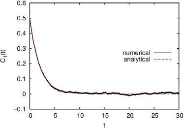
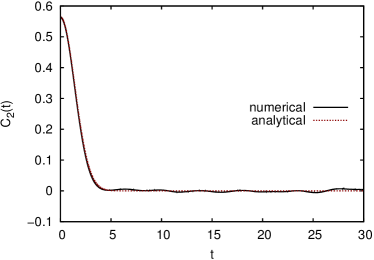
Figure 1: (Color online) Comparison of the numerical simulation of $\langle\xi(0)\xi(t)\rangle$ with the analytical result for two different covariance functions ($C_{1}$, $D=2,\,\tau=2$ and $C_{2}$, $D=2,\,\alpha=2$) based on 8000 realizations.

In this way we have worked out a method to obtain a stationary Gaussian process with an arbitrary covariance function and a positive-valued Fourier transform. Using this approach, the noise can be simulated with only small numerical effort (see the Appendix). The question is now how the covariance function affects the solution of the Langevin equation.

III The generalized Langevin equation

In the following we assume that the collisions experienced by an observed particle in the heat bath are time-correlated with each other resulting in a time-correlated noise for the Langevin equation. Since the stochastic force as well as the friction force in the Langevin equation are of the same origin, the friction force will also have a time dependence. The environment of the particle is affected by its movement and the particle is influenced to a later time in return, i.e., we describe a non-Markovian process with memory. Therefore, we introduce a time-dependent friction kernel $\Gamma(t)$ leading to the following form of the generalized one dimensional Langevin equation Toda et al. (1992):

$$m\ddot{x}(t)+2\int_{0}^{t}\!\mathrm{d}t^{\prime}\,\Gamma(t-t^{\prime})\dot{x}(t^{\prime})-F_{\mathrm{ext}}(x)=\xi(t)\,,$$ (24)

where $F_{\mathrm{ext}}(x)$ is an additional external force. Assuming that the equipartition principle holds,

$$\frac{1}{2}m\langle v^{2}\rangle=\frac{1}{2}T\,,$$

we obtain a relation between the friction kernel $\Gamma(t)$ and the covariance function $C(t)$:

$$\Gamma(t-t^{\prime})=\frac{1}{2T}\langle\xi(t)\xi(t^{\prime})\rangle=\frac{1}{2T}C(t-t^{\prime})\,.$$ (25)

This is the well known fluctuation-dissipation theorem. For an arbitrary time-independent external force $F_{\mathrm{ext}}(x)$ a derivation can be found in Cortés et al. (1985).

Our numerical solving algorithm for the generalized Langevin equation (24) is based on the three-step Adams-Bashforth scheme (Faires and Burden, 2003, p. 307), where the right side is calculated with the method presented in the Appendix. Therefore, for each particle we store the position $x(t)$ and velocity $\dot{x}(t)$ at every time step.

IV Langevin equation without external potential

We first analyze the generalized Langevin equation without an external potential,

$$m\ddot{x}(t)+2\int_{0}^{t}\!\mathrm{d}t^{\prime}\,\Gamma(t-t^{\prime})\dot{x}(t^{\prime})=\xi(t)\,,$$ (26)

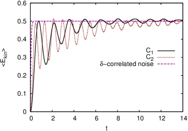
Figure 2: (Color online) Numerical evolution of the mean kinetic energy (26) for the exponential covariance function $C_{1}(t)$ with $\tau=2$, the Gaussian covariance function $C_{2}(t)$ with $\alpha=1$, and the theoretical limit of $\tau\to 0$, $\alpha\to 0$ corresponding to $\delta$-correlated white noise. The initial conditions for both simulations are given in (27).

where for initial conditions we choose

$$x_{0}=0,\quad v_{0}=0,\quad D=2,\quad m=0.1,\quad T=1\,.$$ (27)

We note that these initial conditions imply that this “Brownian particle” is not assumed to be in equilibrium with the “heat bath” represented by the fluctuating force, $\xi$, which is described as stationary Gaussian noise. Consequently the solutions of (26) includes transient motion of the Brownian particle, while the corresponding back reaction to the heat bath is neglected. Indeed, for both covariance functions, $C_{1}(t)$ and $C_{2}(t)$, we obtain an oscillating transient solution of the Langevin equation until the equilibrium value is reached, which differs significantly from the exponential trend in case of $\delta$-correlated white noise (see Fig. 2)Kubo (1966). The oscillation is due to the retarded friction on the particle due to the memory of the system.

IV.1 Analytical solution for $C_{1}$

To solve the generalized Langevin equation (26) analytically as a linear integro-differential equation, we can benefit from a continuation of the velocity $v(t)$ by defining $v_{T}$ as

$$v_{T}(t)=\begin{cases}0\quad&\mathrm{for}\quad t<0\,,\\ v(t)\quad&\mathrm{for}\quad t\in[0,T]\,,\\ v(T)\quad&\mathrm{for}\quad t>T\end{cases}$$ (28)

and choosing $v(0)=0$, such that $v_{T}(t)$ is a continuous function. With

$$\xi_{T}(t)=\begin{cases}0\quad&\mathrm{for}\quad t<0\,,\\ \xi(t)\quad&\mathrm{for}\quad t\in[0,T]\,,\\ 0\quad&\mathrm{for}\quad t>T\\ \end{cases}$$

and

$$\Gamma_{\text{ret}}(t)=\begin{cases}0\quad&\mathrm{for}\quad t<0\,,\\ \Gamma(t)\quad&\mathrm{for}\quad t>0\\ \end{cases}$$

we obtain an equation which is identical to Eq. (26) in the interval $t\in[0,T]$:

$$m\dot{v}_{T}(t)+2\int_{-\infty}^{\infty}\!\mathrm{d}t^{\prime}\,\Gamma_{\mathrm{ret}}(t-t^{\prime})v_{T}(t^{\prime})=\xi_{T}(t)\,.$$

This linear differential equation can be solved with the ansatz

$$m\dot{G}_{\mathrm{ret}}(t)+2\int_{-\infty}^{\infty}\!\mathrm{d}t^{\prime}\,\Gamma_{\mathrm{ret}}(t-t^{\prime})G_{\mathrm{ret}}(t^{\prime})=\delta(t)\,,$$ (29)

where $G_{\mathrm{ret}}(t)$ denotes a retarded Green’s function. The velocity is then given by

$$v_{T}(t)=\int_{-\infty}^{\infty}\!G_{\mathrm{ret}}(t-t^{\prime})\xi_{T}(t^{\prime})\mathrm{d}t^{\prime}\quad\text{for}\quad t\in[0,T]\,.$$ (30)

The Green’s function can be found via a Fourier transform of (29), leading to

$$\tilde{G}_{\text{ret}}(\omega)=\frac{1}{2\tilde{\Gamma}_{\text{ret}}(\omega)-\mathrm{i}m\omega}.$$ (31)

For the exponential covariance function, $C_{1}(t)$, we find

$$\tilde{\Gamma}_{\text{ret}}(\omega)=\frac{D}{4T}\frac{1}{1-\mathrm{i}\omega\tau}$$ (32)

and thus for the retarded Green’s function, according to (31)

$$\begin{split}\tilde{G}_{\text{ret}}(\omega)&=\frac{1}{m\tau}\frac{\mathrm{i}\omega\tau-1}{\omega^{2}+\mathrm{i}\omega/\tau-Q/(2\tau)},\end{split}$$ (33)

where $Q=\frac{D}{mT}$. The Fourier transformation to the time domain is done in the usual way, using the theorem of residues by closing the integration path in the upper (lower) $\omega$-half plane for $t<0$ ($t>0$). As to be expected from the retardation condition, $\tilde{G}_{\text{ret}}$ is analytic in the upper half-plane. For $t>0$ and $2Q\tau<1$, defining $\gamma_{c}=\frac{\sqrt{1-2Q\tau}}{2\tau}$, the Green’s function reads

$$G_{\mathrm{ret}}(t)=\frac{1}{m}\left[\frac{1}{2\gamma_{c}\tau}\sinh(\gamma_{c}t)+\cosh(\gamma_{c}t)\right]\mathrm{e}^{-\frac{t}{2\tau}}.$$ (34)

This can be analytically continued to the case $2Q\tau>1$ by setting $\gamma_{c}=\mathrm{i}\omega_{c}$ with $\omega_{c}=\frac{\sqrt{2Q\tau-1}}{2\tau}$:

$$G_{\mathrm{ret}}(t)=\frac{1}{m}\left[\frac{1}{2\omega_{c}\tau}\sin(\omega_{c}t)+\cos(\omega_{c}t)\right]\mathrm{e}^{-\frac{t}{2\tau}}.$$ (35)

Finally, the case $2Q\tau=1$ can be found by taking the limit $\gamma_{c}\rightarrow 0$ of (34), resulting in

$$G_{\text{ret}}(t)=\frac{1}{m}\left(\frac{t}{2\tau}+1\right)\mathrm{e}^{-\frac{t}{2\tau}}.$$ (36)

For small correlation times, i.e., for $2Q\tau\leq 1$ we find an exponential-decay behavior. The relaxation time is larger compared to the Markovian limit due to the memory effects described by the correlation function. For larger correlation times the system oscillates with the characteristic frequency $\omega_{c}=\frac{\sqrt{2Q\tau-1}}{2\tau}$ due to the memory of the medium, leading to a kind of “plasmon formation”. This is also reflected in the velocity-correlation function, which we evaluate next.

Inserting the Fourier transform of $\tilde{v}_{T}(\omega)$ from Eq. (30),

$$\tilde{v}_{T}(\omega)=\tilde{G}_{\text{ret}}(\omega)\tilde{\xi}_{T}(\omega)$$ (37)

into the definition of the velocity’s spectral density (Coffey et al., 2004, p. 60) yields

$$\begin{split}S_{v}(\omega)&=\lim_{T\to\infty}\frac{1}{T}\left\langle{\lvert\tilde{v}_{T}(\omega)\rvert}^{2}\right\rangle\\ &=\lim_{T\to\infty}\frac{1}{T}{\lvert\tilde{G}_{\mathrm{ret}}(\omega)\rvert}^{2}\left\langle{\lvert\tilde{\xi}_{T}(\omega)\rvert}^{2}\right\rangle\\ &={\lvert\tilde{G}_{\mathrm{ret}}(\omega)\rvert}^{2}S_{\xi}(\omega)=2T{\lvert\tilde{G}_{\mathrm{ret}}(\omega)\rvert}^{2}\tilde{\Gamma}(\omega)\,.\end{split}$$ (38)

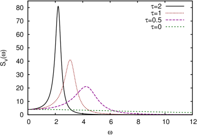
Figure 3: (Color online) The spectral density of the velocity for different correlation times. For small values of $\tau$ the peak becomes broader and is shifted to higher frequencies.

Since $\Gamma(t)=\Gamma(-t)\in\mathbb{R}$, using the definition of the retarded damping function a direct evaluation of its Fourier transform yields ($\omega\in\mathbb{R}$)

$$\tilde{\Gamma}(\omega)=\tilde{\Gamma}_{\text{ret}}(\omega)+\tilde{\Gamma}_{\text{ret}}^{*}(\omega).$$ (39)

Using (33) this can be written as

$$\tilde{\Gamma}=\frac{1}{2}\left(\frac{1}{\tilde{G}_{\text{ret}}}+\frac{1}{\tilde{G}_{\text{ret}}^{*}}\right)=\frac{\operatorname{Re}\tilde{G}_{\text{ret}}}{|\tilde{G}_{\text{ret}}|^{2}},$$ (40)

and with the fluctuation-dissipation relation (25) we finally arrive at

$$\begin{split}S_{v}(\omega)=&2T\,\operatorname{Re}\left[\tilde{G}_{\mathrm{ret}}(\omega)\right]\\ =&\frac{D^{2}}{m^{2}}\,\frac{1}{\frac{1}{4}Q^{2}+(1-Q\tau)\omega^{2}+\tau^{2}\omega^{4}}.\end{split}$$ (41)

Fig. 3 shows the spectral density for different correlation times $\tau$, where for long correlation times we observe a clear oscillation expressed by a sharp peak at the frequency $\omega_{\mathrm{peak}}$, which is given by

$$\omega_{\mathrm{peak}}=\frac{\sqrt{2Q\tau-2}}{2\tau}\,.$$

If $\tau$ is large enough, it follows that $\omega_{\mathrm{peak}}\approx\frac{\sqrt{2Q\tau-1}}{2\tau}=\omega_{c}$. For decreasing $\tau$ the peak becomes broader, and its maximum moves to the right until $\omega_{\mathrm{peak}}$ reaches an extremum for $Q\tau=2$. For very small values of $\tau$ the maximum of the spectral density remains at $0$ and approaches a Lorentz shape with a width of $\frac{\gamma}{m}$ (Xu, 1999, p. 53), Xu and Greiner (2000), where $\gamma=\frac{D}{2T}$ according to the Nernst-Einstein relation. As expected, this leads to the Markovian limit for the Langevin equation with white noise.

For $2Q\tau>1$ we obtain an expression for the mean kinetic energy $\left\langle E_{\mathrm{kin}}(t)\right\rangle$:

$$\begin{split}\left\langle{E_{\text{kin}}}\right\rangle&=\frac{1}{2}m\left\langle v^{2}(t)\right\rangle=\frac{1}{2}m\int_{0}^{t}\!\mathrm{d}s\int_{0}^{t}\!\mathrm{d}s^{\prime}\,G_{\mathrm{ret}}(t-s)G_{\mathrm{ret}}(t-s^{\prime})\left\langle\xi(s)\xi(s^{\prime})\right\rangle\\ &=\frac{1}{2}m\int_{0}^{t}\!\mathrm{d}s\int_{0}^{t}\!\mathrm{d}s^{\prime}G_{\mathrm{ret}}(t-s)G_{\mathrm{ret}}(t-s^{\prime})C(s-s^{\prime})\\ &=\frac{1}{2}T-\frac{1}{2}\frac{T}{2Q\tau-1}\left[Q\tau+\sqrt{2Q\tau-1}\sin(2\omega_{c}t)+(Q\tau-1)\cos(2\omega_{c}t)\right]\mathrm{e}^{-\frac{t}{\tau}},\end{split}$$ (42)

showing the relaxation to the equilibrium value $T/2$ with the damping time $\tau$ and oscillations due to the memory effect.

IV.2 Numerical results

In Fig. 4 we compare the analytical expression of the kinetic energy with the numerical average over 8000 realizations, where the initial conditions are given by

$$x_{0}=0,\quad v_{0}=0,\quad D=2,\quad m=0.1,\quad T=1$$

and $\tau=2$. Our numerical simulation is in a good agreement with the analytical result. Fig. 5 shows the kinetic energy for different values of $\tau$. For a system in equilibrium, we have verified numerically that the velocity of particles is Boltzmann distributed.

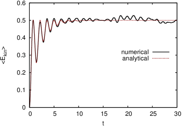
Figure 4: (Color online) Comparison of the kinetic energy between the analytical expression (Eq. (42)) and the numerical average over 8000 realizations.

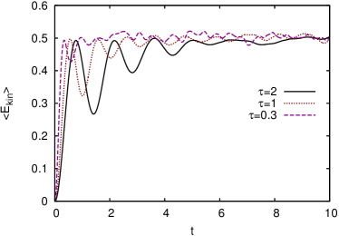
Figure 5: (Color online) Numerical results for the kinetic energy and different values of $\tau$. As expected, with increasing correlation times the system takes longer to approach the equilibrium state.

V Langevin equation in quadratic potentials

In this Section we verify our numerical algorithm to simulate non-Markovian Brownian motion for the analytically solvable case of the motion in quadratic potentials, i.e., the harmonic-oscillator and the quadratic-barrier potential.

V.1 Harmonic-oscillator potential

We now add a harmonic potential

$$V_{\mathrm{ext}}(x)=\frac{1}{2}m\omega_{0}^{2}x^{2}$$ (43)

as a minimal extension to include an external force. In this case the Langevin equation takes the form:

$$m\ddot{x}(t)+2\int_{0}^{t}\!\mathrm{d}t^{\prime}\,\Gamma(t-t^{\prime})\dot{x}(t^{\prime})+m\omega_{0}^{2}x=\xi(t)\,.$$ (44)

From the equipartition and virial theorems we expect

$$\frac{1}{2}m\left\langle v^{2}(t)\right\rangle=\frac{1}{2}m\omega_{0}^{2}\left\langle x^{2}(t)\right\rangle=\frac{1}{2}T\,.$$ (45)

For the initial conditions $x_{0}=0$ and $v_{0}=0$ we can calculate the spectral density of the position $x$ in analogy to the spectral density of the velocity without potential,

$$S_{x}(\omega)={\lvert\tilde{G}_{\mathrm{ret}}(\omega)\rvert}^{2}S_{\xi}(\omega)\,.$$

Here, $\tilde{G}_{\mathrm{ret}}(\omega)$ denotes the retarded Green’s function of $x_{T}(t)$ which solves the equation

$$\begin{split}m\ddot{G}_{\mathrm{ret}}(t)+2\int_{-\infty}^{\infty}\!\mathrm{d}t^{\prime}\,\Gamma_{\mathrm{ret}}(t-t^{\prime})\dot{G}_{\mathrm{ret}}(t^{\prime})&\\ +m\omega_{0}^{2}G_{\mathrm{ret}}(t)=\delta(t)&\,.\end{split}$$ (46)

It can be evaluated in an analogous way as for the free particle cf. Sec. IV, leading to

$$S_{x}(\omega)=\frac{2T}{\omega}\mathrm{Im}[\tilde{G}_{\mathrm{ret}}(\omega)]$$ (47)

with

$$\tilde{G}_{\mathrm{ret}}(\omega)=\frac{1}{m\left(\omega_{0}^{2}-\omega^{2}-i\frac{2\omega}{m}\tilde{\Gamma}_{\mathrm{ret}}(\omega)\right)}\,.$$ (48)

Fig. 6 shows a peak in the spectral density approaching the frequency $\omega_{0}$ for long correlation times $\tau$. For smaller values of $\tau$ the peak becomes broader. The frequency of this peak is denoted with $\omega_{\mathrm{peak}}$, and its development as a function of $\tau$ is shown in Fig. 7. In the present example the damping of the system, characterized by $D$, is relatively large. With decreasing values of $D$ the function of the peak frequency becomes continuous.

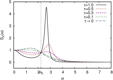
Figure 6: (Color online) Spectral density of the position $x$ in a harmonic oscillator. The simulation parameters are $T=1$, $D=1$, $m=0.2$ and $\omega_{0}=\sqrt{5}$.

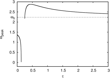
Figure 7: (Color online) Behavior of the peak frequency $\omega_{\mathrm{peak}}$ as a function of $\tau$. In a narrow frequency range the peak vanishes completely. With increasing values of $\tau$ it approaches the frequency of the harmonic oscillator whereas in the limit $\tau\to 0$ its frequency converges to the white-noise limit. The same simulation parameters have been used as in Fig. 6.

V.2 Diffusion over a barrier

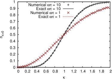
Figure 8: (Color online) Simulation for the probability to pass a square barrier compared to the analytic result (50) Boilley and Lalloet (2006). We use the same representation of the barrier height as in this reference, i.e., $\kappa=K/B_{\text{eff}}$ with $B_{\text{eff}}=B\omega_{0}/\lambda_{1}^{2}$.

As an additional test of our numerical method, we simulate the diffusion of a non-Markovian Brownian particle over a square-barrier potential,

$$V(x)=-\frac{m\omega_{0}^{2}}{2}x^{2}.$$ (49)

As detailed in Boilley and Lalloet (2006), this problem can be solved analytically for the case of the correlation function $C_{1}$ (22). Although the Brownian particle can not come to thermal equilibrium in this case, because the potential is not bounded from below, the probability to pass over the barrier is well defined. With the initial kinetic energy $K=p_{0}^{2}/2m$ ($p_{0}>0$) and the barrier height $B=m\omega_{0}^{2}x_{0}^{2}/2$ ($x_{0}<0$), $\beta=D/(2mT)$ in the here simulated case of a stationary non-Markovian Langevin process it reads for $t\rightarrow\infty$

$$\begin{split}P(x_{0},p_{0})=\frac{1}{2}\mathrm{erfc}\Bigg{[}\omega_{0}&\sqrt{\frac{1+\lambda_{1}\tau}{\beta\lambda_{1}}}\\ &\times\Bigg{(}\sqrt{\frac{B}{T}}-\frac{\lambda_{1}}{\omega_{0}}\sqrt{\frac{K}{T}}\Bigg{)}\Bigg{]}.\end{split}$$ (50)

The parameter $\lambda_{1}$ is the positive root of the cubic equation

$$\lambda^{3}+\frac{\lambda^{2}}{\tau}+\left(\frac{\beta}{\tau}-\omega_{0}^{2}\right)-\frac{\omega_{0}^{2}}{\tau}=0.$$ (51)

To further validate our numerics, we have used the same test cases as in Boilley and Lalloet (2006). As can be seen in Fig. 8, the results of the simulation is in perfect agreement with the analytical result (50). We have checked that further evolution to later times within our numerical simulation does not change the passing probability anymore, i.e., that the time evolution really converges to the anlytical result. We have also verified that the same results can be achieved with the stochastic process, using a white-noise auxiliary variable, as explained in the reference.

VI Langevin equation in a double well potential

Figure 9: (Color online) 400 independent realizations of the Langevin equation (52) with a symmetric double-well potential and initial conditions as defined in (55). Shown is the total energy and position of each particle at the time $t=5$.

The general form of a double-well potential $V(x)$ is described by

$$V(x)=ax^{4}+bx^{3}+cx^{2}+d$$

with a suitable choice of parameters $a$, $b$, $c$ and $d$. Since the corresponding force is not linear in $x$, a linear Green’s function method is no longer applicable to solve the Langevin equation

$$\begin{split}m\ddot{x}(t)&+2\int_{0}^{t}\!\mathrm{d}t^{\prime}\,\Gamma(t-t^{\prime})\dot{x}(t^{\prime})\\ &+4ax^{3}+3bx^{2}+2cx=\xi(t)\,,\end{split}$$ (52)

and we present only numerical results.

VI.1 Symmetric double well potential

Here, we consider a symmetric potential with $b=0$, centered around $x=0$. For an analytic study of the diffusion over a saddle with the generalized Langevin equation, including the exponential covariance function $C_{1}(t)$, see Boilley and Lalloet (2006). All particles are initially located in the left potential minimum, and the initial conditions are (see also Fig. 9)

$$\begin{gathered}x_{0}=x_{\mathrm{minL}},\quad v_{0}=0,\quad D=2,\quad m=0.1,\\ T=1,\quad\Delta V=1,\quad x_{\mathrm{minL}}=-x_{\mathrm{minR}}=-2\,.\end{gathered}$$ (55)

For the exponential covariance function $C_{1}(t)$ the system equilibrates at the expected mean kinetic energy of $\frac{1}{2}T$ as illustrated in Fig. 10. Let $N_{x>0}(t)$ be the number of particles on the right side of the well and $N_{\mathrm{total}}$ the total number of simulated particles. The relative number of particles on the right side is then given by

$$n_{x>0}(t)=N_{x>0}(t)/N_{\mathrm{total}}$$

and is shown for different correlation times $\tau$ in Fig. 11. If the correlation time is large enough, the first particles overcoming the well (steep rise in Fig. 11) are dragged back to the left (drop in Fig. 11) due to the memory effect. When these particles reach the left potential well they are dragged back once more from the left to the right such that we see a rise of $n_{x>0}(t)$ again. This oscillation could go on for a long time if the particles were not influenced by the random force of the heat bath over time, making them “forget” about their history. In the case of a large correlation time $\tau=6$ we can vaguely observe a second drop in the number of particles on the right side.

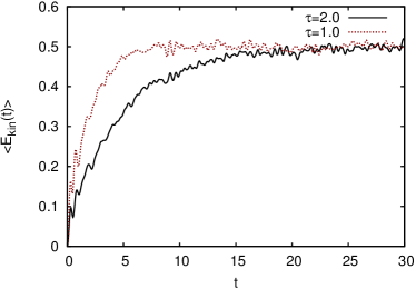
Figure 10: (Color online) Kinetic energy of the Langevin equation (52) with a symmetric double well potential for the covariance function $C_{1}$.

For larger times $t>5$, $n_{x>0}(t)$ follows an exponential growth of the form

$$n_{x>0}(t)=0.5-B\,\exp\left(-\frac{t}{\tau_{\mathrm{eq}}}\right)\,,$$

where $B$ and $\tau_{\mathrm{eq}}$ are two fit parameters, and $\tau_{\mathrm{eq}}$ describes the characteristic time of the system to reach its equilibrium state. Fig. 12 shows a significant increase of $\tau_{\mathrm{eq}}$ as a function of the correlation time $\tau$.

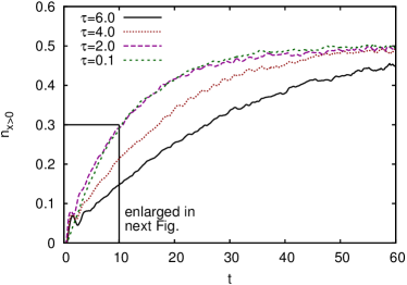
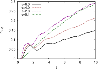
Figure 11: (Color online) Relative number of particles located on the right side of the symmetric potential for different correlation times $\tau$ and two different time ranges.

Figure 12: (Color online) Characteristic time $\tau_{\mathrm{eq}}$ for the system to reach equilibrium in the symmetric double well potential as a function of the correlation time $\tau$.

VI.2 Asymmetric double well potential

Figure 13: (Color online) 400 independent realizations of the Langevin equation (52) with an asymmetric double well potential and initial conditions as defined in (59). Shown is the total energy and position of each particle at the time $t=5$.

If $b\neq 0$, the double-well potential becomes asymmetric as shown in Fig. 13 and can be applied for instance to describe the case of heavy-ion fusion. For an analysis in the white-noise limit see Abe et al. (2000). The initial conditions for the following simulations are

$$\begin{gathered}x_{0}=x_{\mathrm{minL}},\quad v_{0}=0,\quad D=4,\quad m=0.1,\\ (\Delta V)_{\mathrm{L}}=1,\quad(\Delta V)_{\mathrm{R}}\approx 2.90,\\ \quad x_{\mathrm{minL}}\approx-1.83,\quad x_{\mathrm{minR}}\approx 2.73\,.\end{gathered}$$ (59)

With rising temperature some particles fall into the deeper right potential minimum and remain there. For even higher temperatures it is possible that these particles overcome the potential barrier $(\Delta V)_{\mathrm{R}}$ from the right. Fig. 14 and 15 show the development of $n_{x>0}(t)$ for $\tau=0.1$, $\tau=2$ and different values of the temperature. We observe that for very high temperatures the equilibrated relative number of right particles lowers since more particles can overcome the right potential barrier $(\Delta V)_{\mathrm{R}}$ backwards. Fig. 16 shows this development of $n_{x>0}(t)$ for different temperatures at two time values $t=4$ and $t=20$. The effect of the correlation time $\tau$ becomes smaller with increasing $t$.

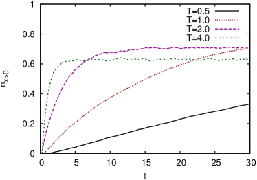
Figure 14: (Color online) Relative number of particles located on the right side of the potential well for different temperatures $T$ and correlation time $\tau=0.1$.

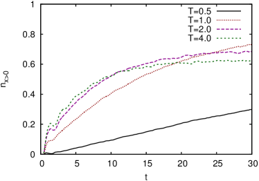
Figure 15: (Color online) Same as Fig. 14 but for the correlation time $\tau=2$.

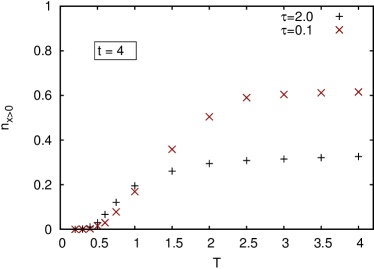
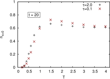
Figure 16: (Color online) Relative number of particles located on the right side of the asymmetric potential well as a function of the temperature $T$ at fixed times $t=4$ (upper figure) and $t=20$ (lower figure). With increasing temperature more particles overcome the potential well in a shorter time. For very high temperatures the particle’s energy becomes large enough to overcome the potential barrier as easily from the right as from the left such that the curve converges to $0.5$. The correlation time has a larger impact on the relative number of particles for smaller times $t$.

VII Conclusion and outlook

In this paper we presented an efficient method to simulate stationary Gaussian noise for an arbitrary covariance function and applied this procedure to the simulation of the generalized Langevin equation with and without external potentials leading to memory effects due to the time correlation of the noise.

In absence of an external potential the memory effect with sufficiently large correlation times realized by different covariance functions manifests itself in “plasmon” oscillations. In the presence of a harmonic potential we are able to solve the Langevin equation in parts analytically and have found an effective particle oscillation frequency composed of an oscillation due to the harmonic potential and an oscillation due to the memory effect. Finally, we presented our numerical results for the simulation of the generalized Langevin equation with a symmetric and an asymmetric double well potential. Here, we emphasize that the correlation of the noise plays an important role in the behavior of the observed particles, leading to memory effects that lead to a delay of the relaxation of quantities like the particle distribution to their equilibrium values.

In this work we mainly focused on the presentation of the generalized Langevin equation including the exponential covariance function $C_{1}(t)$. While the Gaussian covariance function $C_{2}(t)$ also leads to oscillations, the frequencies are different. This motivates for a further study on the impact of different covariance functions.

Another promising investigation with the present method is the question of the diffusion rate (Kramers rate) over a potential barrier Hänggi et al. (1990), which we also postpone to a future publication.

For a more general study of the generalized Langevin equation in three dimensions, with particle-particle interaction, and a memory kernel not only depending on $t-t^{\prime}$ but on $t$ and $t^{\prime}$ separately, see Kantorovich (2008); Stella et al. (2014).

*

Appendix A Algorithm for colored noise

Here, we give explicitly a basic numerical algorithm for generating a sequence of colored noise in accordance with our method, which is described in II.

1. Define a sufficiently large time interval $[-\Delta,\Delta]$, such that all relevant functions (see below for $C(t),G(t)$) become negligibly small outside the interval. Using $(2M+1)$ equidistant grid points on this interval lead then to the following discretized time values and frequency modes:

   $$\begin{split}\Delta t=\frac{\Delta}{M}\,\,&\Rightarrow\,\,t_{m}=m\cdot\Delta t\\ \Delta\omega=\frac{2\pi}{\left(2M+1\right)\Delta t}\,\,&\Rightarrow\,\,\omega_{n}=\frac{2\pi n}{\left(2M+1\right)\Delta t}\end{split}$$ (60)

   with $m,n\in\{-M,...,0,...,M\}$

2. Take the Fourier transform $S_{\xi}(\omega)=\mathcal{F}[C](\omega)$ of the desired covariance function $C(t)$ such as given in (22) on the discrete set of $t$-values:

   $$S_{\xi}\left(\omega_{n}\right)=\Delta t\sum_{m=-M}^{M}C\left(t_{m}\right)\exp(\mathrm{i}\omega_{n}t_{m})\,.$$ (61)

3. Take the inverse Fourier transform of $\sqrt{S_{\xi}(\omega)}$ on the discrete set of $\omega$-values:

   $$G\left(t_{m}\right)=\frac{\Delta\omega}{2\pi}\sum_{n=-M}^{M}\sqrt{S_{\xi}\left(\omega_{n}\right)}\exp(-i\omega_{n}t_{m})\,.$$ (62)

4. Generate a sequence of white noise $\xi_{w}(t)$ on the time interval $[-\Delta,\Delta+T]$:

   $$\xi_{w}(t_{i})=\frac{\bar{a}_{i}}{\sqrt{\Delta t}}\,,$$ (63)

   where $T\geq 0$ defines a time interval for colored noise. The variable $\bar{a}_{i}$ is a standard normally distributed random number.

5. Take the convolution of $G(t)$ with $\xi_{w}(t)$ on the time interval $[-\Delta,\Delta]$ to generate a sequence of colored noise:

   $$\xi(t_{j})=\Delta t\sum_{m=-M}^{M}G\left(t_{m}\right)\xi_{w}\left(t_{j}+t_{m}\right)$$ (64)

   with $t_{j}=j\cdot\Delta t$ for $j\in\{0,..,N\}$ denoting the time points on $[0,T]$.

   We note that for every sequence of colored noise $\xi(t)$ the white noise $\xi_{w}(t)$ has to be generated independently.

References

• Coffey et al. (2004) W. T. Coffey, Y. P. Kalmykov,  and J. T. Waldron, The Langevin Equation: With application to stochastic problems in physics, chemistry and elctrical engineering, 2nd ed., World Scientific Series in Contemporary Chemical Physics, Vol. 14 (World Scientific, Singapure, 2004).
• Xu (1999) Z. Xu, Phänomen der disorientierten chiralen Kondensate in ultrarelativistischen Schwerionenkollissionen, Diploma thesis, University of Gießen (1999).
• Xu and Greiner (2000) Z. Xu and C. Greiner, Phys. Rev. D 62, 036012 (2000).
• Fraga et al. (2006) E. S. Fraga, T. Kodama, G. Krein, A. J. Mizher,  and L. F. Palhares, Phys. Lett. B 614, 181 (2006).
• Nahrgang et al. (2012) M. Nahrgang, S. Leupold,  and M. Bleicher, Phys. Lett. B 711, 109 (2012).
• Herold et al. (2013) C. Herold, M. Nahrgang, I. Mishustin,  and M. Bleicher, Phys. Rev. C 87, 014907 (2013).
• Hijab (2011) O. Hijab, Introduction to Calculus and Classical Analysis, Undergraduate texts in mathematics (Springer New York, 2011).
• Gleiser and Ramos (1994) M. Gleiser and R. O. Ramos, Phys. Rev. D 50, 2441 (1994).
• Rischke (1998) D. H. Rischke, Phys. Rev. C 58, 2331 (1998).
• Farias et al. (2008) R. L. S. Farias, R. O. Ramos,  and L. A. da Silva, Braz. J. Phys 38, 499 (2008).
• Farias et al. (2009) R. L. S. Farias, R. O. Ramos,  and L. A. da Silva, Phys. Rev. E 80, 031143 (2009).
• Greiner and Müller (1997) C. Greiner and B. Müller, Phys. Rev. D 55, 1026 (1997).
• Greiner and Leupold (1998) C. Greiner and S. Leupold, Ann. Phys. 270, 328 (1998).
• Dhar (2008) A. Dhar, Advances in Physics 57, 457 (2008).
• Lü et al. (2012) J. T. Lü, M. Brandbyge, P. Hedegård, T. N. Todorov,  and D. Dundas, Phys. Rev. B 85, 245444 (2012).
• Hänggi et al. (1990) P. Hänggi, P. Talkner,  and M. Borkovec, Rev. Mod. Phys. 62, 251 (1990).
• Harko et al. (2014) T. Harko, C. S. Leung,  and G. Mocanu, Eur. Phys. J. C 74, 2900 (2014).
• Min et al. (2005) W. Min, G. Luo, B. J. Cherayil, S. C. Kou,  and X. S. Xie, Phys. Rev. Lett. 94, 198302 (2005).
• Fraga et al. (2014) E. S. Fraga, G. Krein,  and L. F. Palhares, Physica A 393, 155 (2014).
• Kapusta and Young (2014) J. I. Kapusta and C. Young, Phys. Rev. C 90, 044902 (2014).
• Heer (1972) C. V. Heer, Statistical Mechanics: Kinetic, Theory and Stochastic Process (Academic Press, New York and London, 1972).
• Albin (2003) P. Albin, Stokastika Processer (Studentliteratur, 2003).
• Toda et al. (1992) M. Toda, R. Kubo, N. Saitō,  and N. Hashitsume, Statistical Physics II: Nonequilibrium Statistical Mechanics (Springer-Verlag, Berlin, Heidelberg, 1992).
• Cortés et al. (1985) E. Cortés, B. J. West,  and K. Lindenberg, The Journal of Chemical Physics 82, 2708 (1985).
• Faires and Burden (2003) J. D. Faires and R. L. Burden, Numerical Methods (Brooks/ Cole-Thomson Learning, 2003).
• Kubo (1966) R. Kubo, Rep. Prog. Phys. 29, 255 (1966).
• Boilley and Lalloet (2006) D. Boilley and Y. Lalloet, Jour. Stat. Phys. 125, 473 (2006).
• Abe et al. (2000) Y. Abe, D. Boilley, B. G. Giraud,  and T. Wada, Phys. Rev. E 61, 1125 (2000).
• Kantorovich (2008) L. Kantorovich, Phys. Rev. B 78, 094304 (2008).
• Stella et al. (2014) L. Stella, C. D. Lorenz,  and L. Kantorovich, Phys. Rev. B 89, 134303 (2014).