[Exponentially small splitting with quadratic frequencies]A methodology for obtaining asymptotic estimates for the exponentially small splitting of separatrices to whiskered tori with quadratic frequencies

Amadeu Delshams Departament de Matemàtica Aplicada I, Universitat Politècnica de Catalunya, amadeu.delshams@upc.edu, pere.gutierrez@upc.edu

Marina Gonchenko Institut für Mathematik, Technische Universität Berlin, gonchenk@math.tu-berlin.de

Pere Gutiérrez

This work has been partially supported by the Spanish MINECO-FEDER grant MTM2012-31714 and the Catalan grant 2009SGR859. The author MG has also been supported by the DFG Collaborative Research Center TRR 109 “Discretization in Geometry and Dynamics”.

Introduction

The aim of this work is to provide asymptotic estimates for the splitting of separatrices in a perturbed 3-degree-of-freedom Hamiltonian system, associated to a 2-dimensional whiskered torus (invariant hyperbolic torus) whose frequency ratio is a quadratic irrational number. We show that the dependence of the asymptotic estimates on the perturbation parameter is described by some functions which satisfy a periodicity property, and whose behavior depends strongly on the arithmetic properties of the frequencies.

First, we describe the Hamiltonian system to be studied. It is also considered in [6], as a generalization of the famous Arnold’s example [1], and provides a model for the behavior of a nearly-integrable Hamiltonian system in the vicinity of a single resonance (see [3] for a motivation). In canonical coordinates $(x,y,\varphi,I)\in\mathbb{T}\times\mathbb{R}\times\mathbb{T}^{2}\times\mathbb{R}^{2}$, we consider a perturbed Hamiltonian

$$H(x,y,\varphi,I)=H_{0}(x,y,I)+\mu H_{1}(x,\varphi).$$ (3)

$$H_{0}(x,y,I)=\langle\omega_{\varepsilon},I\rangle+\frac{1}{2}\langle\Lambda I,I\rangle+\frac{y^{2}}{2}+\cos x-1,$$

$$H_{1}(x,\varphi)=\cos x\cdot\sum_{k_{2}\geq 0}\mathrm{e}^{-\rho|k|}\cos(\langle k,\varphi\rangle-\sigma_{k}).$$

For the integrable Hamiltonian $H_{0}$, we consider a vector of fast frequencies

$$\omega_{\varepsilon}=\frac{\omega}{\sqrt{\varepsilon}}\;,\qquad\omega=(1,\Omega),$$ (4)

where the frequency ratio $\Omega$ is a quadratic irrational number. In this way, our system has two parameters $\varepsilon>0$ and $\mu$, but we assume them linked by a relation of kind $\mu=\varepsilon^{p}$, $p>0$ (the smaller $p$ the better). Thus, if we consider $\varepsilon$ as the unique parameter, we have a singular or weakly hyperbolic problem for $\varepsilon\to 0$ (see [3] for a discussion about singular and regular problems).

On the other hand, notice that $H_{0}$ consists of a classical pendulum and $2$ rotors (in the coordinates $x,y$ and $\varphi,I$ respectively). Then, we see that $H_{0}$ has a family of 2-dimensional whiskered tori, with coincident whiskers (invariant manifolds). Such tori can be indexed by the (constant) action $I$, and have frequency vectors $\omega_{\varepsilon}+\Lambda I$. We assume that the matrix $\Lambda$ is such that the condition of isoenergetic nondegeneracy is satisfied (see for instance [6]). Among the tori, we fix our attention on the torus given by $I=0$,

$$\mathcal{T}_{0}:\qquad(0,0,\theta,0),\quad\theta\in\mathbb{T}^{2},$$

whose inner flow is given, in this parameterization, by $\dot{\theta}=\omega_{\varepsilon}$. This torus has a homoclinic whisker (i.e. coincident stable and unstable whiskers),

$$\mathcal{W}_{0}:\qquad(x_{0}(s),y_{0}(s),\theta,0),\quad s\in\mathbb{R},\ \theta\in\mathbb{T}^{2},$$

where $x_{0}(s)=4\arctan\mathrm{e}^{s}$, $y_{0}(s)=2/\cosh s$ (the upper separatrix of the classical pendulum). The inner flow on $\mathcal{W}_{0}$ is given by $\dot{s}=1$, $\dot{\theta}=\omega_{\varepsilon}$ .

Concerning the perturbation $H_{1}$, it is given by a constant $\rho>0$ (the complex width of analyticity in the angles $\varphi$), and phases $\sigma_{k}$ that, for the purpose of this work, can be chosen arbitrarily.

Under the hypotheses described, the hyperbolic KAM theorem (see for instance [8]) can be applied to the perturbed Hamiltonian (3–3). We have that, for $\mu\neq 0$ small enough, the whiskered torus $\mathcal{T}_{0}$ persists with some shift and deformation giving rise to a perturbed torus $\mathcal{T}$, with perturbed local stable and unstable whiskers.

Such local whiskers can be extended to global whiskers $\mathcal{W}^{\rm s}$, $\mathcal{W}^{\rm u}$ but, in general, for $\mu\neq 0$ they do not coincide anymore, and one can introduce a splitting function giving the distance between the whiskers in the directions of the actions $I\in\mathbb{R}^{2}$: denoting $\mathcal{J}^{{\rm s},{\rm u}}(\theta)$ parameterizations of a transverse section of both whiskers, one can define  $\mathcal{M}(\theta):=\mathcal{J}^{\rm u}(\theta)-\mathcal{J}^{\rm s}(\theta)$,  $\theta\in\mathbb{T}^{2}$. In fact, this function turns out to be the gradient of the (scalar) splitting potential:  $\mathcal{M}(\theta)=\nabla\mathcal{L}(\theta)$  (see [2, §5.2], and also [7]).

In (4), we deal with the following 24 quadratic numbers

$$[\bar{1}]\,,[\bar{2}]\,,\;\ldots,\;[\overline{{13}}]\,,[\overline{{1,2}}]\,,\;\ldots,\;[\overline{{1,12}}]\,,$$ (5)

where we denote a quadratic number according to its periodic part in the continued fraction (see (8)).

Next, we establish the main result of this work, providing two types of asymptotic estimates for the splitting, as $\varepsilon\to 0$. One one hand, we give an estimate for the maximal splitting distance, i.e. for the maximum of $\left|\mathcal{M}(\theta)\right|$, $\theta\in\mathbb{T}^{2}$. On the other hand, we show that for most values of $\varepsilon\to 0$ there exist 4 transverse homoclinic orbits, associated to simple zeros $\theta_{*}$ of $\mathcal{M}(\theta)$ (i.e. nondegenerate critical points of $\mathcal{L}(\theta)$) and, for such homoclinic orbits, we obtain an estimate for the transversality of the splitting, given by the minimum eigenvalue (in modulus) of the matrices ${\rm D}\mathcal{M}(\theta_{*})$.

We use the notation $f\sim g$ if we can bound $c_{1}|g|\leq|f|\leq c_{2}|g|$ with positive constants $c_{1},c_{2}$ not depending on $\varepsilon$, $\mu$.

Theorem 1

Assume the conditions described above for the Hamiltonian (3–3), and that $\varepsilon$ is small enough and $\mu=\varepsilon^{p}$, $p>3$. Then, there exist continued functions $h_{1}(\varepsilon)$ and $h_{2}(\varepsilon)$ (defined in (17)), periodic in $\ln\varepsilon$ and satisfying $1\leq h_{1}(\varepsilon)\leq h_{2}(\varepsilon)$, and a positive constant $C_{0}$ (given in (16)), such that:

• for the maximal splitting distance, we have the estimate

  $$\max_{\theta\in\mathbb{T}^{2}}|\mathcal{M}(\theta)|\sim\frac{\mu}{\sqrt{\varepsilon}}\exp\left\{-\frac{C_{0}h_{1}(\varepsilon)}{\varepsilon^{1/4}}\right\};$$

• the splitting function $\mathcal{M}(\theta)$ has exactly 4 zeros $\theta_{*}$, all simple, for all $\varepsilon$ except for a small neighborhood of a finite number of geometric sequences of $\varepsilon$;

• at each zero $\theta_{*}$ of $\mathcal{M}(\theta)$, the minimal eigenvalue of ${\rm D}\mathcal{M}(\theta_{*})$ satisfies

  $$m_{*}\sim\mu\varepsilon^{1/4}\exp\left\{-\frac{C_{0}h_{2}(\varepsilon)}{\varepsilon^{1/4}}\right\}.$$

For the proof of this theorem, we apply the Poincaré–Melnikov method, which provides a first order approximation

$$\mathcal{M}(\theta)=\mu\nabla L(\theta)+\mathcal{O}(\mu^{2})$$ (6)

in terms of the Melnikov potential, which can be defined by integrating the perturbation $H_{1}$ along the trajectories of the unperturbed homoclinic whisker $\mathcal{W}_{0}$ :

$$L(\theta):=-\int_{-\infty}^{\infty}H_{1}(x_{0}(t),\theta+\omega_{\varepsilon}t)\,{\rm d}t.$$ (7)

Since this first order approximation is exponentially small in $\varepsilon$, in principle the approximation (6) cannot be directly applied in our singular problem with $\mu=\varepsilon^{p}$. However, using suitable bounds for the error term $\mathcal{O}(\mu^{2})$, given in [6], one can see that for $p>3$ the first order approximation given by the Melnikov potential overcomes the error term and provides the right asymptotic estimates for the splitting. Such estimates come from the size of dominant harmonics in the Fourier expansion of (7), and studying their dependence on $\varepsilon$. More precisely, to estimate the maximal splitting one dominant harmonic is enough and, to estimate the transversality of the splitting, two dominant harmonics are required (excluding the values of $\varepsilon$ such that the second and third harmonics are of the same magnitude, which could give rise to bifurcations in the homoclinic orbits and would require a further study).

The remaining sections of this work are devoted to the definition of the functions $h_{1}(\varepsilon)$ and $h_{2}(\varepsilon)$, putting emphasis on their dependence on the arithmetic properties of the quadratic number $\Omega$.

Continued fractions and resonant sequences

We review briefly the technique developed in [4] for studying the resonances of quadratic frequencies. Let $0<\Omega<1$ be a quadratic irrational number. It is well-known that it has an infinite continued fraction

$$\Omega=[a_{1},a_{2},a_{3},\ldots]=\frac{1}{a_{1}+\dfrac{1}{a_{2}+\dfrac{1}{a_{3}+\cdots}}}\,,\qquad a_{n}\in\mathbb{Z}^{+},\ n\geq 1\quad\mbox{(and $a_{0}=0$)},$$ (8)

that is that is eventually periodic, i.e., periodic starting at some $a_{l}$. For a purely $m$-periodic continued fraction $\Omega=[\overline{a_{1},\ldots,a_{m}}]$ we introduce the matrix

$$U=(-1)^{m}A_{1}^{-1}\cdots A_{m}^{-1},\textrm{ where }A_{l}=\left(\begin{array}[]{cc}a_{l}&1\\[3.0pt] 1&0\end{array}\right),\;\;\;l=1,\ldots,m.$$

It is well-known that quadratic vectors satisfy a Diophantine condition

$$|\langle k,\omega\rangle|\geq\frac{\gamma}{|k|},\;\;\;\forall k\in\mathbb{Z}^{2}\setminus\{0\}.$$

With this in mind, we define the “numerators”

$$\gamma_{k}:=|\langle k,\omega\rangle|\cdot|k|,\qquad k\in\mathbb{Z}^{2}\setminus\left\{0\right\}$$ (9)

(for integer vectors, we use the norm $\left|\cdot\right|=\left|\cdot\right|_{1}$). Our aim is to find the integer vectors $k$ which give the smallest values $\gamma_{k}$, we call such vectors $k$ the primary resonances.

All vectors $k\in\mathbb{Z}^{2}\setminus\left\{0\right\}$ with $\left|\left\langle k,\omega\right\rangle\right|<1/2$ are subdivided into resonant sequences:

$$s(j,n):=U^{n}k^{0}(j),\qquad n=0,1,2,\ldots$$ (10)

where the initial vector $k^{0}(j)=(-\mathop{\rm rint}(j\Omega),j)$, $j\in\mathbb{Z}^{+}$, satisfies

$$\frac{1}{2\lambda}<|\langle k^{0}(j),\omega\rangle|<\frac{1}{2},$$ (11)

$\lambda$ being the eigenvalue of $U$ with $\lambda>1$. For each $j\in\mathbb{Z}^{+}$ satisfying (11), it was proved in [4, Th. 2] (see also [5]) that, asymptotically, the resonant sequence $s(j,n)$ exhibits a geometric growth and the sequence $\gamma_{s(j,n)}$ has a limit $\gamma^{*}_{j}$:

$$|s(j,n)|=K_{j}\lambda^{n}+\mathcal{O}(\lambda^{-n}),\;\;\;\gamma_{s(j,n)}=\gamma_{j}^{*}+\mathcal{O}(\lambda^{-2n}),\textrm{ as }n\to\infty,$$ (12)

where $K_{j}$ and $\gamma_{j}^{*}$ can be determined explicitly for each resonant sequence (see explicit formulas in [4]). We select the minimal of $\gamma_{j}^{*}$:

$$\gamma^{*}:=\liminf_{|k|\to\infty}\gamma_{k}=\min_{j}\gamma^{*}_{j}=\gamma^{*}_{j_{0}}>0.$$ (13)

The integer vectors of the corresponding sequence $s(j_{0},n)$ are the primary resonances, and we call the secondary resonances the integer vectors belonging to any of the remaining resonant sequences $s(j,n)$, $j\neq j_{0}$. We also call by the main secondary resonances the sequence $s(j_{1},n)$ which is linearly independent with $s(j_{0},n)$ and gives the smallest limit $\gamma^{*}_{j_{1}}$ among the secondary resonances.

The functions $h_{1}(\varepsilon)$ and $h_{2}(\varepsilon)$

Taking into account the form of $H_{1}$ in (3), we present the Melnikov potential (7) in its Fourier expansion. Using (4) and (9), we present the coefficients in the form

$$L_{k}=\frac{2\pi|\langle k,\omega_{\varepsilon}\rangle|\,\mathrm{e}^{-\rho|k|}}{\sinh|\frac{\pi}{2}\langle k,\omega_{\varepsilon}\rangle|}=\alpha_{k}\,\mathrm{e}^{-\beta_{k}},\qquad\alpha_{k}\approx\frac{4\pi\gamma_{k}}{|k|\sqrt{\varepsilon}}\,,\quad\beta_{k}=\rho|k|+\frac{\pi\gamma_{k}}{2|k|\sqrt{\varepsilon}}\,.$$ (14)

For any given $\varepsilon$, we find the dominant harmonics $L_{k}(\varepsilon)$ which correspond essentially to the smallest exponents $\beta_{k}(\varepsilon)$.

The exponents $\beta_{k}(\varepsilon)$ in (14) can be presented in the form

$$\beta_{k}(\varepsilon)=\frac{C_{0}}{\varepsilon^{1/4}}\,g_{k}(\varepsilon),\qquad g_{k}(\varepsilon):=\frac{\tilde{\gamma}_{k}^{1/2}}{2}\left[\left(\frac{\varepsilon}{\varepsilon_{k}}\right)^{1/4}+\left(\frac{\varepsilon_{k}}{\varepsilon}\right)^{1/4}\right],$$ (15)

where

$$\varepsilon_{k}:=D_{0}\,\frac{\tilde{\gamma}_{k}^{\,2}}{\left|k\right|^{4}}\,,\qquad\tilde{\gamma}_{k}=\frac{\gamma_{k}}{\gamma^{*}},\qquad C_{0}=(2\pi\rho\gamma^{*})^{1/2},\qquad D_{0}=\left(\frac{\pi\gamma^{*}}{2\rho}\right)^{2}.$$ (16)

Since the coefficients $L_{k}$ are exponentially small in $\varepsilon$, it is more convenient to work with the functions $g_{k}$, whose smallest values correspond to the largest $L_{k}$. To this aim, it is useful to consider the graphs of the functions $g_{k}(\varepsilon)$, $k\in\mathbb{Z}^{2}\setminus\{0\}$, in order to detect the minimum of them for a given value of $\varepsilon$.

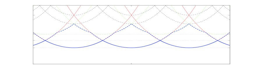
Figure 1: Graphs of the functions $h_{1}(\varepsilon)$ (solid blue) and $h_{2}(\varepsilon)$ (dash-dot blue) for $[\overline{1,2}]=\sqrt{3}-1$. The red lines are the primary functions $g_{s(j_{0},n)}(\varepsilon)$, and the green lines correspond to the main secondary functions $g_{s(j_{1},n)}(\varepsilon)$.

We know from (15) that the functions $g_{k}(\varepsilon)$ have their minimum at $\varepsilon=\varepsilon_{k}$ and the corresponding minimal values are $g_{k}(\varepsilon_{k})=\tilde{\gamma}_{k}^{1/2}$. For the integer vectors $k=s(j,n)$ belonging to a resonant sequence (10), using the approximations (12), we have

$$\varepsilon_{s(j,n)}\approx\frac{D_{0}(\tilde{\gamma}^{*}_{j})^{2}}{K_{j}^{\,4}\lambda^{4n}},\;\;\;g_{s(j,n)}(\varepsilon)\approx\frac{(\tilde{\gamma}^{*}_{j})^{1/2}}{2}\left[\left(\frac{\varepsilon}{\varepsilon_{s(j,n)}}\right)^{1/4}+\left(\frac{\varepsilon_{s(j,n)}}{\varepsilon}^{1/4}\right)\right],\textrm{ as }n\to\infty.$$

Taking into account such approximations, we have a periodic behavior of the functions with respect to $\ln\varepsilon$, as we see in Figure 1 (where a logarithmic scale for $\varepsilon$ is used).

We define, for any given $\varepsilon$, the function $h_{1}(\varepsilon)$ and $h_{2}(\varepsilon)$ as

$$h_{1}(\varepsilon):=\min_{k}g_{k}(\varepsilon)=g_{S_{1}}(\varepsilon),\;\;\;\displaystyle h_{2}(\varepsilon):=\min\limits_{k\ {\rm lin.indep.of}\;S_{1}}g_{k}(\varepsilon)=g_{S_{2}}(\varepsilon),$$ (17)

with some integer vectors $S_{1}(\varepsilon)$ and $S_{2}(\varepsilon)$ realizing such minima. The functions are continuous and $4\ln\lambda$-periodic in $\ln\varepsilon$. It turns out that for the 24 quadratic numbers (5), the integer vector $S_{1}(\varepsilon)$ providing $h_{1}(\varepsilon)$ always corresponds to a primary resonance, defined in (13). On the other hand, the vector $S_{2}(\varepsilon)$ providing $h_{2}(\varepsilon)$ may correspond to primary or main secondary resonances in different intervals of $\varepsilon$ (see Figure 1 for an illustration for the number $[\overline{1,2}]=\sqrt{3}-1$). There is a finite number of geometric sequences of $\varepsilon$, where a change in $S_{2}(\varepsilon)$ occurs. These points require a special study for the transversality and they are excluded in Theorem 1.

References

• [1] V.I. Arnold. Soviet Math. Dokl., 5(3):581–585, 1964.
• [2] A. Delshams and P. Gutiérrez. J. Nonlinear Sci., 10(4):433–476, 2000.
• [3] A. Delshams and P. Gutiérrez. In C.K.R.T. Jones and A.I. Khibnik, editors, Multiple-Time-Scale Dynamical Systems (Minneapolis, MN, 1997), volume 122 of IMA Vol. Math. Appl., pages 1–27. Springer-Verlag, New York, 2001.
• [4] A. Delshams and P. Gutiérrez. Zap. Nauchn. Sem. S.-Peterburg. Otdel. Mat. Inst. Steklov. (POMI), 300:87–121, 2003. (J. Math. Sci. (N.Y.), 128(2):2726–2746, 2005).
• [5] A. Delshams, M. Gonchenko, and P. Gutiérrez. Electron.Res.Ann.Math.Sci., 21:41–61, 2014.
• [6] A. Delshams, P. Gutiérrez, and T.M. Seara. Discrete Contin. Dyn. Syst., 11(4):785–826, 2004.
• [7] L.H. Eliasson. Bol. Soc. Brasil. Mat. (N.S.), 25(1):57–76, 1994.
• [8] L. Niederman. J. Differential Equations, 161(1):1–41, 2000.