Nature and Raman signatures of the Higgs (amplitude) mode
in the coexisting superconducting and charge-density-wave state

Abstract

We investigate the behavior of the Higgs (amplitude) mode when superconductivity emerges on a pre-existing charge-density-wave state. We show that the weak overdamped square-root singularity of the amplitude fluctuations in a standard BCS superconductor is converted in a sharp, undamped power-law divergence in the coexisting state, reminiscent of the Higgs behavior in Lorentz-invariant theories. This effect reflects in a strong superconducting resonance in the Raman spectra, both for an electronic and a phononic mechanism leading to the Raman visibility of the Higgs. In the latter case our results are relevant to the interpretation of the Raman spectra measured experimentally in NbSe₂.

I Introduction

The emergence of collective excitations after spontaneous breaking of a continuous symmetry is the mechanism at the heart of the mass generation for scalar and vector bosons in the Standard Model.weinberg ; higgs_discovery Its direct analogous in condensed matter physics is the appearance of two collective modes as fluctuations of the macroscopic (complex) order parameter in a superconducting (SC) system.nagaosa Indeed, amplitude fluctuations, which are energetically costly, represent the analogous of the Higgs field, and phase fluctuations, which are massless at long wavelengths, represent the Goldstone mode that can be gauged away to make the electromagnetic field massive, leading to the Meissner effect. Interestingly, the first experimental evidence of the Higgs particlehiggs_discovery occurred simultaneously to a renewed interest in the literature on the behavior of the Higgs mode in condensed-matter systems,varma_cm14 like e.g.superfluid cold atomspodolsky_prb11 ; prokofev_prl12 ; podolsky_prl13 ; coldatoms1 ; coldatoms2 , where it can be excited by shaking the optical latticecoldatoms1 ; coldatoms2 .

On the other hand, in conventional BCS superconductors the Higgs mode is usually very elusive, for two concomitant reasons. From one side, in contrast to Lorentz-invariant bosonic theories, in BCS superconductors the amplitude fluctuations do not identify a sharp power-law resonance, but only a weak square-root singularity at twice the SC gap $\Delta$,volkov73 ; kulik81 that is strongly overdamped by quasiparticle excitations. Thus, even in a fully-gapped superconductor, the Higgs-mode spectral function is a broad feature peaked exactly at the edge $2\Delta$ where also single-particle excitations start to develop. In addition, in the weak-coupling BCS limit the Higgs mode is expected to couple weakly to typical spectrosocpic observables, like the current, probed by means of optical measurement, and the charge, probed by means of Raman spectroscopy. Indeed, the Higgs mode is a scalar, so it does not couple directly to the current, unless disorder breaks translational invariancecea_prb14 , and it couples weakly to the charge, due to the intrinsic particle-hole symmetry enforced by the BCS solution. Thus, unless one strongly perturbs the system out of equilibrium,shimano ; carbone ; shimano14 the Higgs resonance remains hidden in conventional superconductors.

An exception to this rule seems to be the case of NbSe₂, a low-temperature superconductor ($T_{c}=7$K) where superconductivity emerges after a charge-density-wave (CDW) transition at higher temperature $T_{CDW}=33$ K. In this material a strong resonance in the Raman responseklein_prl80 ; sacuto_prb14 appears below $T_{c}$ at about $2\Delta$. As suggested long ago within a phenomenological model by Littelewood and Varma,varma_prb82 and within a more microscopic approach by Brouwne and Levin,brouwne_prb83 this peak can be assigned to the Higgs mode. Indeed, according to this interpretation the pre-existing CDW state provides a soft phonon, Raman active already below $T_{CDW}$,tsang_prl76 that below $T_{c}$ couples also to the Higgs mode. As a consequence, the phonon response itself carries out a signature of the SC amplitude mode, that becomes sharp since it is pushed slightly below the treshold $2\Delta$ of quasiparticle excitations. In other words, the current theoretical understanding is that the pre-existing CDW state is crucial to provide a mechanism of Raman visibility of the Higgs mode, but is does not change its nature.

This interpretation seems to be supported by the recent observationsacuto_prb14 that no sharp peak appears in the isostructural superconducting NbS₂, which lacks CDW order. On the other hand, the overall strength of the Higgs resonance in the experiments is much larger than what predicted by the previous theoretical work,varma_prb82 ; brouwne_prb83 especially when one takes into account residual damping effects, neglected so far. In addition, the Higgs signature shows a still unexplained dependence on the Raman light polarization,sacuto_prb14 that could be used instead to solve the still on-going debate on the symmetry of the CDW and SC gaps in this material.arpes1 ; arpes2 ; arpes3 ; arpes4 ; arpes5

In the present paper we address the above issues by unveiling the real character of the Higgs fluctuations in the mixed CDW-SC state. As a first result we show that in a CDW superconductor the CDW contributes crucially to modify the Higgs mode itself, making its detection easier whatever is the mechanism making it physically observable. By computing the Higgs mode in a microscopic CDW+SC model we show that the presence of a CDW gap above the SC one pushes the quasiparticle continuum away from the Higgs pole at $2\Delta$, transforming the weak (overdamped) square-root singularity of a conventional BCS superconductor in a well-defined power-law divergence. Thus, even in the weak-SC-coupling limit, the amplitude mode in the CDW+SC state resembles closely the one found in Lorentz-invariant relativistic theories, suitable in the bosonic limit.podolsky_prb11 ; prokofev_prl12 ; podolsky_prl13 This result has its own interest in the current discussion on the nature of Higgs fluctuations in condensed-matter systems, and it could be further tested by non-equilibrium spectroscopy, where a direct non-linear coupling of the electromagnetic field to the amplitude mode can be generated.shimano14 Second, we compute explicitly the Raman response of the Higgs mode both in the absence and in the presence of an intermediate CDW phonon. In the former case the coupling of the amplitude fluctuations to the Raman response is not zero when computed in a lattice mode, but still very small. While in an ordinary superconductor this would still lead to a negligible visibility of the strongly overdamped Higgs mode, in the CDW case the modified Higgs spectral function will emerge naturally as a strong resonance. In the case where a CDW phonon is also present the computation of the Raman response requires to account for the intermediate electronic processes that make the CDW phonon itself Raman visible below $T_{CDW}$. This mechanism is analogous to the one discussed e.g. for the Raman-active phonons in CDW dichalcogenidesnagaosa_raman ; klein_raman82 or for the optical-active phonons in carbon-based compoundsrice_76 and few-layers graphene.kuzmenko ; li ; cappelluti_prb12 When this effect is taken into account one finds that the double-peak (phonon+Higgs) Raman structure emerging below $T_{c}$ has in general a non-trivial temperature and polarization dependence. These results suggest that the recent observations of a polarization dependence of the Higgs signatures in the Raman spectra of NbSe₂sacuto_prb14 can be used to disentangle the underlying symmetry of the two CDW and SC order parameters in this material.

The structure of the paper is the following. In Section II we introduce the microscopic SC+CDW model and we compute the Higgs spectral function in the mixed state, showing its remarkable difference with the case of a conventional superconductor. In Section III we analyze instead the Raman response, in the case where the CDW has an electronic (Sec. IIIA) or phononic (Sec. IIIB) origin. In both cases we explain all the microscopic mechanisms making the Higgs and/or the phonon Raman visible, and we stress the effect of a modified Higgs mode on the Raman response. The final remarks are discussed in Section IV. In Appendix A we discuss the differences and analogies between the coupling of the Higgs mode to the charge density and the Raman density, respectively. Finally, Appendix B contains some results for the present model away from half-filling, to show the robustness of our conclusions in a regime where an analyitical interpretation of the numerical results cannot be given.

II Higgs mode in the coexisting CDW+SC state

As discussed in the Introduction, to make progress with respect to previous workvarma_prb82 ; brouwne_prb83 we need two ingredients: (i) an overlap bewteen the SC and CDW gaps and (ii) a lattice model, crucial to account for the Raman-polarization effects. To minimize the resulting technical complications we choose here a single-band model on the square lattice (lattice spacing $a=1$) with band dispersion $\xi_{\bf k}\equiv\varepsilon_{\bf k}-\mu=-2t(\cos k_{x}+\cos k_{y})-\mu$ , where $t=1$ is the hopping (that fixes the energetic units from now on) and $\mu$ is the chemical potential. Near half filling ($\mu=0$) the nesting of the Fermi surface at the CDW vector ${\bf Q}=(\pi,\pi)$ allows for a CDW instability to occur, with new bands $\xi_{\pm}=-\mu\mp\sqrt{\varepsilon_{\bf k}^{2}+D_{0}^{2}\gamma_{\bf k}^{2}}$. Here we model it with an order parameter $D_{0}=W\sum_{{\bf k}\sigma}\langle\gamma_{\bf k}c^{\dagger}_{{\bf k}\sigma}c_{{\bf k}+{\bf Q}\sigma}\rangle$, where the $\gamma_{\bf k}=|\cos k_{x}-\cos k_{y}|$ factor modulates the CDW in the momentum space, so that below $T_{CDW}$ the Fermi surface consists of small pockets around $(\pi/2,\pi/2)$. This feature is reminiscent of the situation in NbSe₂, where ARPES experimentsarpes1 ; arpes2 ; arpes3 ; arpes4 ; arpes5 reported the presence of ungapped Fermi arcs below $T_{CDW}$. Here the coupling $W$ can be thought to originates either from an electronic interaction or from the coupling to a phonon, as we shall discuss in Sec. IIB below. The superconductivity originates from a BCS-like interaction term $H_{SC}=-(U/N)\sum_{q}\Phi_{\Delta}^{\dagger}({\bf q})\Phi_{\Delta}({\bf q})$, where $\Phi_{\Delta}({\bf q})\equiv\sum_{\bf k}c_{-{\bf k}+{\bf q}/2\downarrow}c_{{\bf k}+{\bf q}/2\uparrow}$ is the pairing operator and $N$ is the number of lattice sites. When treated at mean-field level it leads to the following Green’s function $G_{0}^{-1}(\mathbf{k},i\omega_{n})$, defined on the basis of a generalized 4-components Nambu spinor $\Psi^{\dagger}_{\bf k}(i\omega_{n})\equiv(c^{\dagger}_{\mathbf{k}\uparrow}(i\omega_{n}),c^{\dagger}_{\mathbf{k}+\mathbf{Q}\uparrow}(i\omega_{n}),c_{-\mathbf{k}\downarrow}(-i\omega_{n}),c_{-\mathbf{k}-\mathbf{Q}\downarrow}(-i\omega_{n}))$ that accounts for the CDW band folding:

$$G_{0}^{-1}(\mathbf{k},i\omega_{n})\equiv i\omega_{n}-\begin{pmatrix}\hat{h}&&-\Delta_{0}\sigma_{0}\\ -\Delta_{0}\sigma_{0}&&-\hat{h}\end{pmatrix},$$ (1)

where $\Delta_{0}$ is the SC gap, $\sigma_{i}$ denotes the Pauli matrices and $\hat{h}$ is a $2\times 2$ matrix:

$$\hat{h}=\begin{pmatrix}\varepsilon_{\bf k}-\mu&&-D_{0}\gamma_{\bf k}\\ -D_{0}\gamma_{\bf k}&&-\varepsilon_{\bf k}-\mu\end{pmatrix}.$$ (2)

The eigenvalues of the matrix $\hat{h}$ represent the two CDW bands $\xi_{\pm}$, while in the SC state the full Green’s function (1) has four possible poles, corresponding to the energies $\pm E_{\pm}({\bf k})$, with $E_{\pm}=\sqrt{\xi_{\pm}^{2}+\Delta_{0}^{2}}$. We note in passing that a similar model (but with $d$-wave symmetry of the SC order parameter) has been the subject of intense investigation in the past within the context of cuprate superconductors, as a potential model for a CDW-like pseudogap phase. nota_ddw

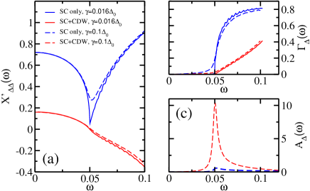
Figure 1: Frequency dependence of the real (a) and imaginary (b) part of the Higgs spectral function (c) at $T=0$ in the presence (SC+CDW) and in the absence (SC only) of CDW, for a quasiparticle damping $\gamma=0.016\Delta_{0}$ (solid lines) and $\gamma=0.1\Delta_{0}$ (dashed lines). Here $\Delta_{0}=0.025$, as in Fig. 2

.

To study the SC fluctuations we derive the effective action for the collective modes by means of the usual Hubbard-Stratonovich decoupling of $H_{SC}$.benfatto_prb04 After integration of the fermions one is left with an action $S=S_{MF}+S_{FL}$ for the collective SC degrees of freedom only, where $S_{MF}={N\Delta_{0}^{2}}/{TU}-\mathrm{Tr}\log G_{0}^{-1}$ is the mean-field action and $S_{FL}[\Delta,\theta]$ is the action for the amplitude $\Delta$ and phase $\theta$ fluctuations around the BCS solution (1) above. With respect to the usual case here the presence of a CDW instability introduces in general in $S_{FL}$ a finite coupling between the SC fluctuations at ${\bf q}$ and ${\bf q}+{\bf Q}$, see Appendix B. However, one can show that this coupling vanishes at half-filling, so for the sake of simplicity we will discuss in the following this case. At the same time, in the SC+CDW state the amplitude and phase/charge fluctuations remain decoupled at Gaussian level, as it occurs in the usual weak-coupling SC state,varma_prb82 ; benfatto_prb04 so we can neglect them in what follows (see also discussion in Appendix A). The Gaussian action for the amplitude SC fluctuations then reads

$$S_{FL}=\frac{1}{2}\sum_{q}\left(\frac{2}{U}+\chi_{\Delta\Delta}(q)\right)|\Delta(q)|^{2},$$ (3)

where $\chi_{\Delta\Delta}$ is the response function for the amplitude operator $\Phi_{\Delta}$ and $q=({\bf q},\Omega_{n})$, with $\Omega_{n}$ bosonic Matsubara frequencies. The behavior of the amplitude fluctuations is controlled by the function $X_{\Delta\Delta}\equiv 2/U+\chi_{\Delta\Delta}$ in Eq. (3), since $\langle|\Delta(q)|^{2}\rangle=1/X_{\Delta\Delta}$. In analogy with the usual SC casekulik81 one can replace the term $2/U=2\sum_{\bf k}\tanh(\beta E_{\bf k}/2)/E_{\bf k}$ by means of the self-consistent equation for $\Delta_{0}$, in order to get:

$$X_{\Delta\Delta}=\frac{2}{U}+\chi_{\Delta\Delta}=\frac{2}{N}\sum_{\bf k}\frac{(i\Omega_{n})^{2}-4\Delta_{0}^{2}}{E_{\bf k}[(i\Omega_{n})^{2}-4E_{\bf k}^{2}]}\tanh({\beta E_{\bf k}}/{2})$$ (4)

where the summation is restricted to the reduced Brillouin zone and $E_{\bf k}=E_{\pm}=\sqrt{\varepsilon_{\bf k}^{2}+\Delta_{0}^{2}+D_{0}\gamma_{\bf k}^{2}}$. In first approximation one can estimate the integral (4) at $T=0$ by assuming that both the density of states $N_{0}$ and the CDW gap are constant (i.e. $\gamma_{\bf k}=1$). In this case one can easily obtain that for $\omega\lesssim 2\Delta_{0}$:

$$X^{\prime}_{\Delta\Delta}\simeq(4\Delta_{0}^{2}-\omega^{2})\frac{N_{0}\mathrm{atan}(\Delta_{0}/D_{0})}{\omega\sqrt{4D_{0}^{2}+4\Delta_{0}^{2}-\omega^{2}}}.$$ (5)

In the pure SC case ($D_{0}=0$) the denominator diverges as a square-root at $\omega=2\Delta_{0}$,kulik81 signaling the proliferation of single-particle excitations above this threshold, and $X^{\prime}_{\Delta\Delta}\sim\sqrt{4\Delta_{0}^{2}-\omega^{2}}$ near the Higgs mass $\omega=2\Delta_{0}$. In contrast, in the mixed state the CDW gap pushes the quasiparticle continuum away from the Higgs mode, leading to a finite denominator in Eq. (5). This implies a linear vanishing of $X^{\prime}_{\Delta\Delta}$ at $2\Delta_{0}$ and suppresses its imaginary part $\Gamma_{\Delta}\equiv-X"_{\Delta\Delta}$. These simple estimates are confirmed by the numerical calculation done for the real band dispersion, as shown in Fig. 1a,b, where we report both $X^{\prime}_{\Delta\Delta}$ and $\Gamma_{\Delta}$ in the two cases, with and without preformed CDW state. To account also for residual quasiparticle scattering we added a finite constant broadening $\gamma$ in the response functions. As one can see in Fig. 1a, in the SC+CDW state $X^{\prime}_{\Delta\Delta}$ vanishes approximately linearly, in contrast to the square-root of the usual SC casekulik81 computed with the same $\Delta_{0}$, and $\Gamma_{\Delta}$ (see Fig. 1b) develops smoothly above $2\Delta_{0}$, since only few quasiparticle excitations in the regions with small CDW gap contribute to it. These two concomitant effects lead to a dramatic sharpening of the Higgs spectral function $A_{\Delta}(\omega)=(1/\pi)\mathrm{Im}X_{\Delta\Delta}^{-1}(i\Omega_{n}\rightarrow\omega+iO^{+})$

$$A_{\Delta}\equiv\frac{1}{\pi}\frac{\Gamma_{\Delta}(\omega)}{X_{\Delta\Delta}^{{}^{\prime}2}(\omega)+\Gamma_{\Delta}^{2}(\omega)},$$ (6)

shown in Fig. 1c for the case $\gamma=0.1\Delta$. While in the ordinary SC state we recover the typical overdamped structure of the amplitude fluctuations, in the CDW+SC state the Higgs mode becomes a well-defined excitation, rather insensitive to residual quasiparticle excitations, that are pushed away from the Higgs pole by the CDW gap. As we show in Appendix B, the same qualitative features survive also at finite doping, even if part of the Fermi surface remains ungapped below $T_{CDW}$. The strong modifications of the Higgs spectral function shown in Fig. 1c, and due to the emergence of superconductivity on the pre-existing CDW state, represent the first crucial result of our work. Indeed, they imply that whatever is the mechanism that couple the Higgs mode to a physical observable, its detection in the mixed state becomes easier since the mode itself is much sharper than in an ordinary superconductor. As an example of this mechanism we will discuss in the next Section the case of the Raman response.

III Raman signatures of the Higgs mode

III.1 Electronic mechanism

We first compute the Raman spectra in the case where the CDW has an electronic origin, so that the Raman visibility of the Higgs can only be due to a direct coupling between the SC amplitude fluctuations and the Raman charge fluctuations. Within the effective-action formalism the Raman response can be computed by introducing in the fermionic model a source term $\rho_{R}$ coupled to the Raman density operator $\Phi_{R}(\mathbf{q})\equiv\sum_{\mathbf{k}\sigma}\Gamma(\mathbf{k})c^{\dagger}_{\mathbf{k}-\mathbf{q}/2,\sigma}c_{\mathbf{k}+\mathbf{q}/2,\sigma}$. Here $\Gamma(\mathbf{k})$ is the Raman vertex, determined by the polarization of the incident and scattered photonreview . After integration of the fermions $\rho_{R}$ appears as an additional bosonic field in the action $S_{FL}$, that now reads

$$S_{FL} = \frac{1}{2}\sum_{q}\left\{\left(\frac{2}{U}+\chi_{\Delta\Delta}(q)\right)|\Delta(q)|^{2}+\right.$$ (7)

$$+ \left.2\rho_{R}(q)\Delta(-q)\chi_{R\Delta}(q)+|\rho_{R}(q)|^{2}\chi^{0}_{RR}(q)\right\}.$$

Here $\chi_{AB}(q)$ denotes the response functions computed with the $A,B$ operators, where $R$ identifies the Raman density $\Phi_{R}$, $\Delta$ the pairing operator $\Phi_{\Delta}$, and $\chi_{RR}^{0}$ represents the BCS Raman response function in the absence of the collective modes. Notice that even if one included explicitly the Coulomb forces the Raman response here would be unaffected, since phase fluctuations do not couple to the Raman response at ${\bf q}=0$, while charge fluctuations, that in general screen $\chi^{0}_{RR}$ in the symmetric $A_{1g}$ channel, review are ineffective in the present model since the charge-Raman coupling vanishes exactly at half-filling because of particle-hole symmetry. Finally, the Raman response is obtained by analytical continuation $i\Omega_{n}\rightarrow\omega+i\delta$ as $S_{R}=-\frac{1}{\pi}[1+n(\omega)]\chi_{RR}^{\prime\prime}({\bf q}=0,\omega)$, where $n(\omega)$ the Bose-Einstein distribution and $\chi_{RR}$ is the Raman susceptibility, computed from Eq. (7) as:

$$\chi_{RR}(q)=\left[\frac{\delta^{2}{S}_{FL}}{\delta\rho_{R}(-q)\delta\rho_{R}(q)}\right]_{\rho_{R}=0}\quad.$$ (8)

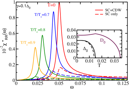
Figure 2: Electronic Raman response in the $A_{1g}$ channel in the coexisting (solid lines) and pure (dashed lines) SC state as a function of temperature. Inset: temperature evolution of the SC gaps $\Delta_{0}$ and of the CDW gap $D_{0}$.

By integrating out explicitly the amplitude fluctuations in Eq. (7) we are then left with the Raman response:

$$\chi_{RR}=\chi_{RR}^{0}-{\chi^{2}_{R\Delta}}/X_{\Delta\Delta},$$ (9)

where the second term, depicted in Fig. 3a, is equivalent to compute the RPA vertex corrections due to amplitude fluctuations.review The coupling of the Higgs to the Raman density is mediated by the fermionic susceptibility $\chi_{R\Delta}$:

$$\chi_{R\Delta}=\frac{8\Delta_{0}}{N}\sum_{\bf k}\frac{\Gamma({\bf k})\varepsilon_{\bf k}\tanh(\beta E_{\bf k}/2)}{E_{\bf k}[(i\Omega_{n})^{2}-4E_{\bf k}^{2}]},$$ (10)

that is finite in the $A_{1g}$ channel where $\Gamma({\bf k})=(\cos k_{x}+\cos k_{y})\propto\varepsilon_{\bf k}$. Since in the $A_{1g}$ channel the BCS contribution $\chi^{0}_{RR}$ is negligible, for this symmetry the Raman response probes essentially the spectral function $A_{\Delta}$ of the Higgs mode given by Eq. (6):

$$\chi^{\prime\prime}_{RR}\simeq\pi\chi^{{}^{\prime}2}_{R\Delta}(\omega)A_{\Delta}(\omega),$$ (11)

leading to the results of Fig. 2 for the CDW+SC (solid lines) and SC only (dashed lines) case. As we discuss in detail in the Appendix A, the coupling $\chi_{R\Delta}$ of the Raman response to the Higgs is in general different from the coupling of the real charge density to SC amplitude fluctuations, that vanishes at weak coupling due to the approximate particle-hole symmetry of the BCS solution.varma_prb82 ; benfatto_prb04 On the other hand, in a ordinary SC state even if this is a finite quantity it multiplies a strongly overdamped Higgs spectral function (see dashed lines in Fig. 1c), so the overall Raman signature of the Higgs is the broad and weak feature represented by dashed lines in Fig. 2. This justifies on microscopic grounds the general expectationvarma_cm14 that the Higgs mode is irrelevant in the Raman spectra of an ordinary superconductor. However, in a CDW+SC state the situation is radically different, since the spectral function itself of the Higgs mode is sharper than usual. Thus, even if in the coexisting state the $\chi_{R\Delta}$ prefactor in Eq. (11) is smaller than in the usual SC state (see Appendix B), the modifications of the Higgs spectral function $A_{\Delta}(\omega)$ shown in Fig. 1 lead to the sharp resonance at $2\Delta_{0}(T)$ shown in Fig. 2. In other words, the CDW state is not modifying the mechanism coupling the Higgs to the Raman probe, but it is changing dramatically the nature of the Higgs mode itsefl, making it detectable.

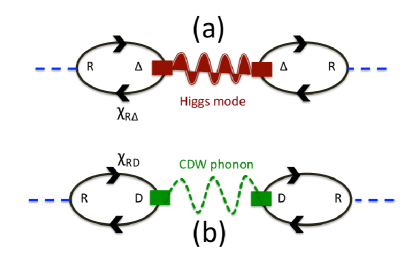
Figure 3: Feynman diagrams representing the electronic processes responsible for the Raman visibility of (a) the Higgs mode when $g=0$ and (b) the CDW phonon above $T_{c}$. Here the dashed lines represent the incoming electromagnetic radiation, the full lines the electronic Green’s functions $G_{0}$, the red and green wavy lines the Higgs propagator $X^{-1}_{\Delta\Delta}(\omega)$ and the phonon one $D(\omega)$, respectively. In the coexistence state for $g\neq 0$ the two processes become interconnected, since both the phonon propagator (see Eq. (15)) and the $\chi_{RD}$ (see Eq. (17)) are renormalized by the coupling bewteen the Higgs fluctuations and the CDW amplitude fluctuations.

III.2 Phononic mechanims

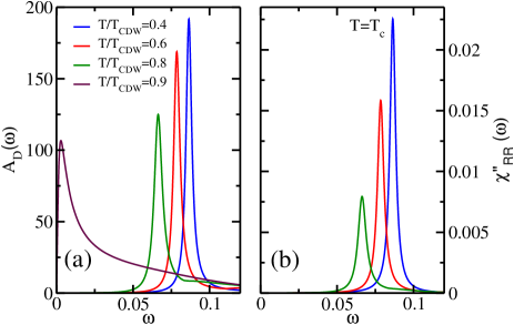
Figure 4: Temperature evolution of the phonon spectral function (a) and of the Raman response (b) of the CDW phonon between $T_{CDW}$ and $T_{c}=0.4T_{CDW}$.

A second possible mechanism that makes the Higgs mode visible in Raman is the one proposed long ago in the case of NbSe₂,varma_prb82 ; brouwne_prb83 where Higgs fluctuations come along with the CDW phonon. To explore also this possibility we then consider the case where the CDW instability is driven by the microscopic coupling of the electrons to a phonon of energy $\omega_{0}$, $H_{I}=g\sum_{{\bf k}\sigma}\gamma_{\bf k}c^{\dagger}_{{\bf k}+{\bf Q}\sigma}c_{{\bf k}\sigma}(b^{+}_{\bf Q}+b_{-{\bf Q}})$, so that $4g^{2}/\omega_{0}$ is equivalent to the coupling $W$ used so far. At mean-field level the description of the CDW+SC state is then identical to the one of Sec. II, and the SC amplitude fluctuations are described by the same effective action (3) derived above, leading to the results of Fig. 1. However, in the calculation of the Raman spectra we should account for two additional effects: (i) the Raman response of the CDW phonon itselfnagaosa_raman ; klein_raman82 and (ii) the coupling between the phonon and the Higgs, that reflects in a renormalization of the phonon propagator.varma_prb82 ; brouwne_prb83 Since all these issues have been discussed only in part in the previous literature, we will outline the basic steps leading to the calculation of the Raman response in this case.

Let us first focus on the regime below $T_{CDW}$ but above $T_{c}$. When the CDW is driven by a lattice instability the energy $\omega_{0}$ of the phonon is renormalized to the value $\Omega_{0}$ by the amplitude fluctuations of the CDW.rice_ssc74 The renormalized phonon propagator below $T_{CDW}$ is then $D^{-1}(i\Omega_{n})=-(\Omega_{n}^{2}+\Omega_{0}^{2})/2\omega_{0}$ with

$$\Omega_{0}^{2} = \omega_{0}^{2}\left[1+\frac{2g^{2}}{\omega_{0}}\chi_{DD}\right]=$$ (12)

$$= \frac{4g^{2}\omega_{0}}{N}\sum_{\bf k}\gamma_{\bf k}^{2}\frac{(i\Omega_{n})^{2}-4D_{0}^{2}\gamma_{\bf k}^{2}}{E_{\bf k}((i\Omega_{n})^{2}-4E_{\bf k}^{2})}\tanh(\beta E_{\bf k}/2),$$

where, in accordance to our notation, the subscript $D$ labels the CDW amplitude operator $\Phi_{D}=\sum_{{\bf k}\sigma}\gamma_{\bf k}(c^{\dagger}_{{\bf k}\sigma}c_{{\bf k}+{\bf Q}\sigma}+h.c.)$. The second line of Eq. (12) has been derived by using the self-consistency equation for the CDW gap, i.e. $1=(4g^{2}/\omega_{0}N)\sum_{\bf k}[\gamma_{\bf k}^{2}\tanh(\beta E_{\bf k}/2)]/E_{\bf k}$. By comparison with Eq. (4) one sees that $\Omega_{0}^{2}$ scales as the inverse propagator of the CDW amplitude fluctuations, that is itself massless at about $4D_{0}$ (where the additional factor of two comes from the $\gamma_{\bf k}$ modulation factor). As a consequence, the renormalized phonon energy also follows the $T$ dependence of the CDW order parameter, so it vanishes at $T=T_{CDW}$ and it is reduced with respect to $\omega_{0}$ at $T=0$,rice_ssc74 as shown by the phonon spectral function $A_{D}(\omega)=-(1/\pi)\mathrm{Im}D(i\Omega_{n}\rightarrow\omega+i\delta)$ reported in Fig. 4a. Notice that, in contrast to previous work,rice_ssc74 ; brouwne_prb83 we retained here the full frequency dependence of $\Omega_{0}$, crucial as $T$ increases and $D_{0}\rightarrow 0$. Thus, the pole of the phonon propagator is determined self-consistently after analytical continuation as as a solution of the equation $\omega^{2}-\Omega_{0}^{2}(\omega)=0$.

The formation of the CDW state is also responsible for the Raman visbility of the phonon. Indeed, in analogy with what suggested for CDW dichalcogenidesnagaosa_raman ; klein_raman82 , the particle-hole excitations at ${\bf q}=0$ probed by Raman couple to the electronic CDW fluctuations at ${\bf Q}$, that in turn can decay in a phonon, as depicted by the process of Fig. 3b. The Raman response of the phonon above $T_{c}$ is then given by

$$\chi_{RR}(i\Omega_{n})=-g^{2}\chi_{RD}^{2}D(i\Omega_{n})=-\frac{2g^{2}\omega_{0}\chi^{2}_{RD}}{\Omega_{0}^{2}-(i\Omega_{n})^{2}},$$ (13)

where

$$\chi_{RD}={8D_{0}}\sum_{\bf k}\frac{\Gamma({\bf k})\gamma_{\bf k}^{2}\varepsilon_{\bf k}}{E_{\bf k}((i\Omega_{n})^{2}-4E_{\bf k}^{2})}\tanh(\beta E_{\bf k}/2),$$ (14)

In full analogy with the case of the $\chi_{R\Delta}$ function that makes the Higgs mode Raman visible, the $\chi_{RD}$ susceptibility depends on the combined symmetry of the Raman polarization, controlled by $\Gamma({\bf k})$, the lattice structure and the CDW symmetry. In the present case one can easily see that Eq. (14) is different from zero only in the $A_{1g}$ channel, where $\Gamma({\bf k})\propto\varepsilon_{\bf k}$. Since $\chi_{RD}$ scales as the CDW order parameter $D_{0}$, the overall temperature evolution of the Raman response (13) of the phonon, shown in Fig. 4b, differs considerably from the one of the spectral function. Indeed, as $T\rightarrow T_{CDW}$ the $\chi_{RD}$ vanishes rapidly (see inset of Fig. 6a) and the Raman response is completely suppressed, in agreement with the experimental observation in NbSe₂.tsang_prl76 It is also worth noting that the crucial role played by the intermediate particle-hole excitations to control the spectroscopic visibility of a phonon is a well-known effect in the literature. For example, in the context of optical conductivity this is the so-called charged-phonon effect, originally introduced by Rice for carbon-based compoundsrice_76 , and widely discussed in the last few years within the context of few-layers graphene.kuzmenko ; li ; cappelluti_prb12 In this case it has been shown that the strong doping dependence of the phonon-peak intensity and its Fano-like shapekuzmenko ; li can be explained by computing the optical visibility of the phonon coming from the process analogous to the one depicted in Fig. 3, with the Raman vertex replaced in this case by the current vertex.cappelluti_prb12

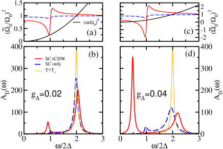
Figure 5: Renormalization of the phonon frequency (a,c) and of the phonon spectral function $A_{D}$ (b,d) due to the Higgs mode according to the phenomenological approach by LV,varma_prb82 where the phonon self-energy is $\Sigma_{\Delta}=-2g^{2}_{\Delta}\chi_{\Delta\Delta}/UX_{\Delta\Delta}$. The Higgs fluctuations $X_{\Delta\Delta}$ are computed in the two cases, with (solid red lines) or without (dashed blue lines, as done in Ref. [varma_prb82, ]) a preformed CDW, and correspond to the data of Fig. 1 for $\gamma=0.1\Delta_{0}$. Here the CDW phonon has energy $\Omega_{0}=4\Delta_{0}$ and $\delta=0.1\Delta_{0}$, leading to the spectral function at $T>T_{c}$ shown by the thin orange line in panels (b) and (d). When entering the SC phase the phonon peak at $\Omega_{0}$ gets broader and slightly displaced, while a second peak develops below $2\Delta_{0}$ due to the Higgs self-energy $\Sigma_{\Delta}$, that causes a second intersection for the curve $\omega^{2}-\tilde{\Omega}_{0}^{2}$ in the inverse phonon propagator.

Below $T_{c}$ the opening of the SC gap modifies both the Raman response, that now inlcudes also the contribution (9) of the Higgs mode, and the phonon propagator itself, that gets renormalized by the SC amplitude fluctuations.varma_prb82 ; brouwne_prb83 The latter mechanism was proposed originally by Littlewood and Varma (LV),varma_prb82 who introduced a phenomenological coupling $g_{\Delta}$ bewteen the Higgs and the phonon. By following the language of LV, one can then write the phonon propagator $D$ in the mixed state as $D^{-1}(\Omega_{n})=-\frac{\Omega_{n}^{2}+\tilde{\Omega}_{0}^{2}}{2\Omega_{0}}$, where $\tilde{\Omega}_{0}^{2}=\Omega_{0}^{2}[1-2\Sigma_{\Delta}/\Omega_{0}]$ is the phonon energy renormalized by the coupling of the phonon to Higgs fluctuations, so that $\Sigma_{\Delta}(\omega)=-2g_{\Delta}^{2}{\chi_{\Delta\Delta}(\omega)}/{UX_{\Delta\Delta}}$. Since near $2\Delta_{0}$ one has $\chi^{\prime}_{\Delta\Delta}\simeq-2/U$ while $X^{\prime}_{\Delta\Delta}\rightarrow 0$, as shown in Fig. 1, the pole of the phonon propagator determined as usual by $\omega^{2}-\tilde{\Omega}^{2}(\omega)=0$ has a new solution around the frequency of the Higgs mode, see Fig. 5a,c. Once more the nature of the Higgs, encoded in $X^{\prime}_{\Delta\Delta}$ and $\Gamma_{\Delta\Delta}$, gives qualitative and quantitative differences if one applies the above phenomenological approach by using the standard form of the Higgs fluctuations, as done by LV, or the real one in the coexisting SC+CDW state. These differences are elucidated in Fig. 5, where we show the renormalized phonon frequency $\tilde{\Omega}_{0}$ and the phonon spectral function for two values of the phenomenological coupling $g_{\Delta}$ and a residual phonon broadening $\delta=0.1\Delta_{0}$ above $T_{c}$. Here the Higgs fluctuations in the two cases (SC and SC+CDW) correspond to the calculations shown in Fig. 1 for $\gamma=0.1\Delta_{0}$. As one can see, for the same remaining parameters a weak feature found for conventional Higgs fluctuations turns out in a strong feature when the Higgs is computed in the mixed state.nota_varma Notice that the crucial role of the residual damping $\gamma$ has been neglected so far,varma_prb82 ; brouwne_prb83 while it is certainly present in real materials and suppresses the signature of a conventional Higgs mode even when the coupling to the phonon moves it inside the quasiparticle continuum. Thus, already this phenomenological approach shows that it is crucial to retain the real nature of the Higgs mode in the coexisting state in order to explain the strong signatures observed experimentally.sacuto_prb14

As shown later on by Browne and Levin (BL), the effective coupling $g_{\Delta}$ between the phonon and the Higgs arises microscopically by the coupling between the amplitude fluctuations of both the CDW and SC order parameter, so that the phonon propagator below $T_{c}$ reads:

$$D^{-1}(i\Omega_{n})=-\frac{\Omega_{0}^{2}-(i\Omega_{n})^{2}-2g^{2}\omega_{0}\chi_{D\Delta}^{2}/X_{\Delta\Delta}}{2\omega_{0}}$$ (15)

where the function

$$\chi_{D\Delta}=-{8D_{0}\Delta_{0}}\sum_{\bf k}\frac{\gamma_{\bf k}^{2}}{E_{\bf k}((i\Omega_{n})^{2}-4E_{\bf k}^{2})}\tanh(\beta E_{\bf k}/2)$$ (16)

is the one that mediates the effective coupling between the phonon and the Higgs fluctuations. It is worth noting that in their paper, BL use a model where the SC and CDW order parameters coexist only on some fraction $\eta$ ($\gamma$ in the notation of Ref. [brouwne_prb83, ]) of the Fermi surface. In the limit when $\eta\rightarrow 0$ BL notice that their result reproduces the one by LV: indeed, in this limit the Higgs mode is the standard one, since in Eq. (5) above there is no CDW gap above the SC one to push the quasiparticle continuum away from the Higgs pole. When instead $\eta$ increases BL observe some numerical difference with respect to the results of LV, that they uncorrectly attribute to a larger value of the effective coupling to the phonon, i.e. the function $\chi_{D\Delta}$ in Eq. (16). However, this is not the case: indeed, even if a larger overlap bewteen the SC and CDW order parameters leads to an increase of $\chi_{D\Delta}$, the stronger effect in the formation of the coexistence state is in the profound modification of the Higgs spectral function. This is clearly shown in Fig. 5, where the two cases (Higgs mode computed with or without the CDW gap) are compared by keeping the same effective coupling $g_{\Delta}$ of the phonon to the Higgs.

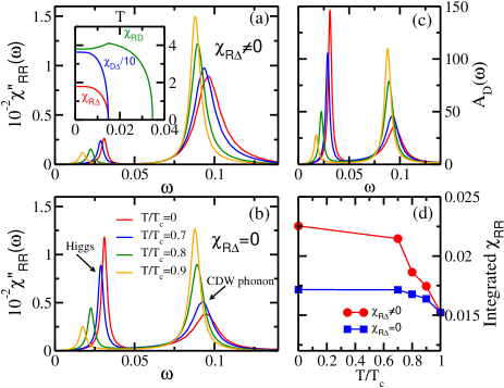
Figure 6: Raman response in the $A_{1g}$ channel in the mixed CDW+SC state according to Eq. (17), both in the presence (a) and in the absence (b) of the direct Raman coupling to the Higgs, encoded in $\chi_{R\Delta}$. The double-peak structure found below $T_{c}$ in the phonon spectral function, shown in panel (c), is weighted in the Raman response by the two polarization functions $\chi_{R\Delta}$ and $\chi_{RD}$. Their value at $\omega=0$ is shown in the inset of panel (a), along with the coupling $\chi_{D\Delta}$ between the two order parameters responsible for the Higgs siganture in the phonon mode. (d) Temperature evolution of the Raman spectral weight integrated between $\omega=0$ and $\omega=0.15$, for the two cases of panels (a)-(b).

Once clarified the role of the modified Higgs fluctuations on the phonon spectral function we now present the results for the Raman response in the coexisting state. As one can easily see, the coupling (16) between the two order parameters renormalizes also the intermediate process $\chi_{RD}$ making the phonon Raman visible, so that the full Raman response reads:

$$\chi_{RR} = -\frac{\chi^{2}_{R\Delta}}{X_{\Delta\Delta}}-\frac{2g^{2}\omega_{0}\left[\chi_{RD}-\frac{\chi_{R\Delta}\chi_{\Delta D}}{X_{\Delta\Delta}}\right]^{2}}{\Omega_{0}^{2}-(i\Omega_{n})^{2}-2g^{2}\omega_{0}\chi_{D\Delta}^{2}/X_{\Delta\Delta}},$$ (17)

where the first term corresponds to the response (9) of the Higgs alone and the second one accounts for the response (13) of the phonon mode, renormalized by the Higgs fluctuations according to Eq. (15). The temperature evolution of the Raman spectra is shown in Fig. 6a for the $\Delta_{0}$, $D_{0}$ appearing in Fig. 1-2. In agreement with the discussion above, the phonon spectral function, shown in Fig. 6c, shows a double-peak structure evolving with temperature, one around $\Omega_{0}$ and one below $2\Delta_{0}$, that is the signature of the Higgs mode. However, the way these two peaks appear in the Raman response depends crucially on the polarization functions $\chi_{RD}$ and $\chi_{R\Delta}$, see Fig. 6a,b. In particular, by comparing the results of Fig. 6a with the ones in panel b, when we put by hand $\chi_{R\Delta}=0$, one sees that the direct coupling $\chi_{R\Delta}$ of the Higgs to the light is crucial to establish the Raman spectral-weight distribution below $T_{c}$. Indeed, when $\chi_{R\Delta}=0$ the Higgs feature at $T=0$ is stronger than in the case of $\chi_{R\Delta}\neq 0$, shown in Fig. 6a, and the broadening of the phonon peak is also smaller. Both effects are due to the vanishing of the second term in square brackets of Eq. (17), that partly screens out the response at the Higgs when present. Nonetheless, the increase of the Raman spectral weight integrated up to $\omega\simeq 0.15$, shown in Fig. 6d, is larger when $\chi_{R\Delta}\neq 0$, due to a larger broadening of the phonon in this case. Notice also that from Eq. (17) one immediately sees that the peak at the Higgs due to the first term of Eq. (17), and represented in Fig. 2 for the case $g=0$, cancels out here with the second term. Thus in this case the Higgs becomes visible only trough its coupling to the phonon, but its direct visibility $\chi_{R\Delta}$ still influences the overall shape of the Raman spectra.

The crucial difference between the behavior of the Raman response and the behavior of the phonon propagator in a phonon-induced CDW transition has been completely overlooked in the previous work.varma_prb82 ; brouwne_prb83 For example, the claim usually donevarma_prb82 ; brouwne_prb83 that the transfer of spectral weight bewteen the two peaks in the phonon spectral function $A_{D}$ must be found also in the Raman spectra is not correct. In general, this is not the case, as the comparison bewteen the panels a,b,c of Fig. 6 clearly demonstrates. This simple fact can also be used to explain the polarization dependence of the Higgs signatures reported recently in NbSe₂.sacuto_prb14 Indeed, even though our model is not intended to give a realistic description of NbSe₂, nonetheless some general conclusions can be drawn from our results that can be used to interpret the Raman experiments. The general results of our calculations in the case of a phonon-mediated Higgs response can be summarized in three separate items. First, the overlap bewteen the CDW and SC order parameter in part of the Fermi surface is necessary to give rise to a finite $\chi_{D\Delta}$ function in Eq. (16), that controls the effective coupling between the CDW phonon and the Higgs, see Eq. (15). In turn, larger is the fraction of Fermi surface where the overlap occurs and stronger is the enhancement of the Higgs mode itself, shown in Fig. 1, that helps its visibility. Second, both the phonon and the Higgs become Raman visible trough an intermediate electronic processes, given by $\chi_{RD}$ and $\chi_{R\Delta}$ respectively, see Fig. 3. These two functions depend on the combined symmetry of the (CDW or SC) gap and of the Raman light polarization. Thus, different Raman symmetry will give in general a different result, since both functions will acquire a specific frequency and temperature dependence. As a consequence, the differences observed experimentally in NbSe₂ by means of the various Raman symmetriessacuto_prb14 can be used to extract specific informations on the response functions $\chi_{RD}$ and $\chi_{R\Delta}$, and in turn on the gaps themselves.

IV Discussion and Conclusions

The present work focuses on two different problems: the nature of the Higgs mode in the coexisting CDW+SC state, and the issue of its detection in Raman spectroscopy. The first result, discussed in Sec. II, is that in the coexisting CDW+SC state the CDW gap pushes the quasiparticle excitations away from the Higgs pole. Thus, in contrast to the usual SC case, the Higgs mode presents a sharp spectral function, whose detection can be easier, whatever is the mechanism that couples it to a physical observable. It is also interesting that the power-law divergence of the amplitude fluctuations at twice the SC gap value resembles the behavior of the Higgs mode predicted in relativistic ${\cal O}(N)$ theories,podolsky_prb11 ; prokofev_prl12 ; podolsky_prl13 that are expected to work for superfluids or strongly-coupled superconductors. A possible way to test directly our prediction could be for example an out-of-equilibrium optical experiment, where a non-linear coupling of the current to the Higgs can be generated.shimano14 Indeed, in this case we expect that the strongly reduced damping of the Higgs mode in the coexisting state will lead to a much slower decay of the amplitude oscillations with respect to the conventional superconductors investigated so far.shimano ; shimano14 It is also worth noting that the mechanism outlined here can also have a potential impact on the detection of the Higgs mode in other families of superconductors. For example in cuprate superconductors, where signatures of a $2\Delta_{0}$ oscillations in out-of-equilibrium spectroscopy have been also reported, carbone the pseudogap in the quasiparticle excitations present already above $T_{c}$ could contribute to enhance the Higgs fluctuations. Indeed, as mentioned above, a model similar to the one studied in the present paper has been studied long ago as a simplified phenomenological description of a CDW-like pseudogap phase.nota_ddw The quantitative effect on the Higgs should be however estimated within realistic models, since in these materials the quasiparticle continuum extends up to zero frequency due to the $d$-wave nature of the order parameter. Finally, it can be worth exploring also the nature of the Higgs fluctuations in the coexisting spin-density-wave and superconducting state, a situation realized nowadays is some families of iron-based superconductors.review_pnictides

The second part of the paper focuses on the Raman detection of the Higgs mode. Here the final results depend crucially on the nature of the CDW instability itself, as due to an electronic interaction or to the coupling to a phonon. In the former case one probes directly the Higgs spectral function, so a signature at $2\Delta_{0}$ appears in the Raman response, while in the latter case the Higgs signature moves below $2\Delta_{0}$ due to the coupling to the phonon. In both cases one sees that when damping effects, neglected in the previous literature,varma_prb82 ; brouwne_prb83 are taken into account, it is crucial to consider the modified nature of the Higgs mode in the coexisting state in order to resolve the Higgs signatures in the experiments. Moreover, we clarified how the Raman response depends crucially on the intermediate electronic processes that make the Higgs or the phonon Raman visible. This issue, that is often overlooked in the literature,varma_prb82 ; brouwne_prb83 ; varma_cm14 explains the origin of the direct Raman visibilty of the Higss and the transfer of spectral weight between the phonon and Higgs peak. In particular, we suggest that our results can be used as a guideline to infer useful information on the still unsolved issue of the symmetry of the CDW and SC gaps in NbSe₂.

V Acknowledgements

We thank M. Méasson, C. Castellani and J. Lorenzana for useful discussions and suggestions. We acknowledge financial support by MIUR under the projects FIRB-HybridNanoDev-RBFR1236VV, PRIN-RIDEIRON-2012X3YFZ2 and Progetto Premiale 2012-ABNANOTECH.

Appendix A Coupling of the Higgs mode to Raman in a lattice model

In this Appendix we clarify the role played by the intermediate electronic process $\chi_{R\Delta}$ that couples the Higgs mode to the Raman charge density, see Fig. 3a. In particular, we show that at weak SC coupling the coupling of the SC amplitude fluctuations to the Raman charge fluctuations ($\chi_{R\Delta}$) or to the real charge fluctuations ($\chi_{\rho\Delta}$) can be different from each other. Such a difference is crucial since these two quantities play, as we shall see, a quite different role.

Let us first discuss the coupling of the Higgs mode to real charge fluctuations in an ordinary SC, i.e. without preformed CDW state. By means of the standard definition of charge operator $\rho({\bf q})\equiv\sum_{{\bf k}\sigma}c^{\dagger}_{{\bf k}-{\bf q}/2,\sigma}c_{{\bf k}+{\bf q}/2,\sigma}$, one can easily find the well knownranderia ; benfatto_prb04 result that:

$$\chi_{\rho\Delta}=\frac{4\Delta_{0}}{N}\sum_{\bf k}\frac{\xi_{\bf k}\tanh(\beta E_{\bf k}/2)}{E_{\bf k}[(i\Omega_{n})^{2}-4E_{\bf k}^{2}]}.$$ (18)

where $\xi_{\bf k}=\varepsilon_{\bf k}-\mu$ is a generic band dispersion and $E_{\bf k}=\sqrt{\xi_{\bf k}^{2}+\Delta_{0}^{2}}$. In the weak-coupling limit the above integral is dominated by the region around the Fermi level, $\xi_{\bf k}=0$. As a consequence, for any band structure one can assume that the above integral vanishes because of the particle-hole symmetry of the integration limits enforced by the BCS solution, that allows one to put $\chi_{\rho\Delta}\simeq N_{0}\Delta_{0}\int_{-\infty}^{\infty}d\xi\,\xi/[\sqrt{\xi^{2}+\Delta_{0}^{2}}(\omega^{2}-4\xi^{2}-4\Delta_{0}^{2})]=0$. In general, the particle-hole symmetry of the fermionic bubbles in the BCS limit is also evocated to guarantee that amplitude and charge/phase fluctuations are uncoupled at Gaussian level, as we mentioned above Eq. (3), allowing one to study the amplitude sector independently from the charge one. The situation is instead radically different at strong coupling, as discussed e.g. in Ref. [randeria, ; benfatto_prb04, ].

When one computes instead the coupling of the Higgs mode to the Raman charge fluctuations $\rho_{R}({\bf q})\equiv\sum_{{\bf k}\sigma}\Gamma({\bf k})c^{\dagger}_{{\bf k}-{\bf q}/2,\sigma}c_{{\bf k}+{\bf q}/2,\sigma}$ one should consider the additional momentum modulation of the charge provided by the polarization dependent factor $\Gamma({\bf k})$. Thus, even remaining within a BCS scheme $\chi_{R\Delta}$ can be different from zero even if $\chi_{\rho\Delta}\simeq 0$. This can be seen easily in our model, where the two quantities $\chi_{R\Delta}$ and $\chi_{\rho\Delta}$ at half filling are given respectively by Eq. (10) and:

$$\chi_{\rho\Delta}=\frac{4\Delta_{0}}{N}\sum_{\bf k}\frac{\varepsilon_{\bf k}\tanh(\beta E_{\bf k}/2)}{E_{\bf k}[(i\Omega_{n})^{2}-4E_{\bf k}^{2}]},$$ (19)

where now $E_{\bf k}=\sqrt{\varepsilon_{\bf k}^{2}+\Delta_{0}^{2}+D_{0}\gamma_{\bf k}^{2}}$. As a consequence in our case, where the band structure is particle-hole symmetric, at half filling $\chi_{\rho\Delta}$ is exactly zero and it reamains negligibly small away from it. On the other hand, as we mentioned in the text, in the $A_{1g}$ channel where $\Gamma({\bf k})=(\cos k_{x}+\cos k_{y})\propto\varepsilon_{\bf k}$ the integral (10) that defines $\chi_{R\Delta}$ is finite. Indeed, for a constant CDW gap, Eq. (19) at $T=0$ can be approximately estimated as $\chi_{\rho\Delta}\sim\Delta_{0}N_{0}\int d\varepsilon\,\varepsilon/[\sqrt{\varepsilon^{2}+R^{2}}(\omega^{2}-4\varepsilon^{2}-4R^{2})]=0$ while $\chi_{R\Delta}\sim\Delta_{0}N_{0}\int d\varepsilon\,\varepsilon^{2}/[\sqrt{\varepsilon^{2}+R^{2}}(\omega^{2}-4\varepsilon^{2}-4R^{2})]\neq 0$, where $R^{2}=\Delta_{0}^{2}+D_{0}^{2}$. Notice that to appreciate this difference it is crucial to retain a full lattice description of the problem, that has been neglected in the previous theoretical approach.varma_prb82 ; brouwne_prb83

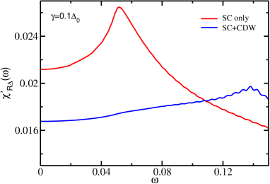
Figure 7: Real part of the Raman response function $\chi_{R\Delta}$ at $T=0$ in the pure SC and in the coexistence SC+CDW state for a residual $\gamma=0.1\Delta_{0}$, as in Fig. 1 and Fig. 2. As one can see, in the mixed CDW+SC case $\chi^{\prime}_{R\Delta}$, that appears as a prefactor in the Raman susceptibility (11), is featureless at the frequency $2\Delta_{0}$ where the Higgs spectral function shown in Fig. 1c has a maximum.

In summary, in our description of the CDW+SC state we can still safetly neglect all the complicationsranderia ; benfatto_prb04 of the coupling between the amplitude mode and the charge/density one, since we are still in a weak-coupling scheme where $\chi_{\rho\Delta}\simeq 0$ at all dopings, but we can retain a finite coupling of the Higgs to the Raman probe, encoded in $\chi_{R\Delta}\neq 0$. In this respect, the general claim done in Ref. [varma_cm14, ] that the Higgs mode is decoupled by the Raman spectra because of particle-hole symmetry is formally uncorrect. However, it is still true that $\chi_{R\Delta}$ is a small quantity, so when the Higgs is an overdamped mode, as in an ordinary superconductor, the overall effect of amplitude fluctuations on the Raman response will be negligible, see dashed lines in Fig. 2. In the CDW+SC state instead the modifications of the Higgs spectral function $A_{\Delta}$ can make this small coupling $\chi_{R\Delta}$ crucial, leading to the strong Raman response represented by the solid lines in Fig. 2. We notice also that the enhancement of the Raman response in the mixed state occurs here despite the fact that $\chi_{R\Delta}$ itself is smaller in the coexisting state, as shown in Fig. 7, due to the presence of the CDW gap. In other words, as we emphasized above, the crucial role of the CDW for what concerns the Raman response is not to enhance the visibility itself of the Higgs, encoded in the electronic process $\chi_{R\Delta}$ (that is indeed even suppressed). The CDW changes crucially the nature of the Higgs spectral function, making the Higgs detectable even in the presence of a small coupling to the Raman light.

Appendix B Variation of the Higgs mode with doping

To elucidate the effect of the CDW gap on the Higgs mode in the case where a larger part of the Fermi surface remains ungapped below $T_{CDW}$ we show here the analogous calculations of Fig. 2 of the manuscript away from half-filling. In our model the CDW gap decreases when one moves away from half-filling, due to the lack of perfect nesting. If one keeps the SC coupling $U$ fixed this reflects also in a rapid increase of the SC order parameter at $T=0$, as shown in Fig. 8a. However, in order to make the comparison between different dopings meaningful, we decided here to reduce also $U$ with doping, in order to retain an almost constant SC gap, see Fig. 8b. This allows one to compare the effects on the Higgs mode due only to the increase of the quasiparticle contribution starting at $2\Delta_{0}$, while keeping $\Delta_{0}$ almost fixed.

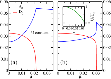
Figure 8: Doping variation of the CDW and SC gap at $T=0$ in the case of a constant (a) or varying (b) SC coupling $U$. In (b) $U$ decreases slightly with doping with respect to the value $U_{0}$ at $\mu=0$ (see inset), in order to reproduce a weaker increase of $\Delta$ with doping.

As mentioned in Sec. II, when one moves away from half-filling the general form of the effective action is more complicated than Eq. (7) of the manuscript, since one should retain in principle also the coupling of the amplitude mode at ${\bf q}=0$ and ${\bf q}={\bf Q}$. One can then show that the Raman response reads:

$$\chi_{RR}(q)=\left[\mathcal{M}^{0}_{RR}(q)-\mathcal{M}_{\Delta R}(q)\mathcal{M}^{-1}_{\Delta\Delta}\mathcal{M}^{T}_{\Delta R}(-q)\right]_{11}$$ (20)

where the matrices $\mathcal{M}^{0}_{RR}$, $\mathcal{M}_{\Delta R}$ and $\mathcal{M}_{\Delta\Delta}$ correspond to the BCS term, to the Higgs-Raman coupling and to the Higgs fluctuations, respectively, with:

$$\mathcal{M}^{0}_{RR}(q)\equiv\begin{bmatrix}\Lambda^{\Gamma\Gamma}_{3333}(q)&&\Lambda^{\tilde{\Gamma}\Gamma}_{1333}(q)\\ \\ \Lambda^{\Gamma\tilde{\Gamma}}_{3313}(q)&&\Lambda^{\tilde{\Gamma}\tilde{\Gamma}}_{1313}(q)\end{bmatrix},$$ (21)

$$\mathcal{M}_{\Delta R}(q)\equiv\begin{bmatrix}\Lambda^{\Gamma}_{0133}(q)&&\Lambda^{\Gamma}_{1133}(q)\\ \\ \Lambda^{\tilde{\Gamma}}_{0113}(q)&&\Lambda^{\tilde{\Gamma}}_{1113}(q)\end{bmatrix},$$ (22)

$$\mathcal{M}_{\Delta\Delta}(q)\equiv\begin{bmatrix}\frac{2}{U}+\Lambda_{0101}(q)&&\Lambda_{1101}(q)\\ \\ \Lambda_{0111}(q)&&\frac{2}{U}+\Lambda_{1111}(q)\end{bmatrix}.$$ (23)

The fermionic susceptibilities $\Lambda_{ijkl}(q)$ are defined as

$$\Lambda_{ijkl}(q)\equiv\frac{T}{N}\sum_{k}\text{Tr}\left[G_{0}(k+q)\sigma_{i}\otimes\sigma_{j}G_{0}(k)\sigma_{k}\otimes\sigma_{l}\right],$$ (24)

and the superscripts $\Gamma,\tilde{\Gamma}$ refer to the insertion of a Raman vertex $\Gamma({\bf k})$ or $\tilde{\Gamma}({\bf k})\equiv\Gamma({\bf k}+{\bf Q}/2)$.

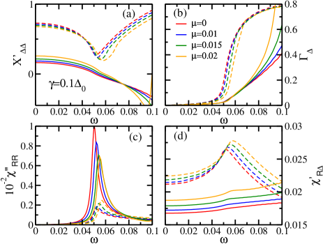
Figure 9: Frequency dependence of the real (a) and imaginary (b) part of the inverse amplitude mode at $T=0$ for different doping levels. In the CDW+SC state the gaps are taken from Fig. S8b, while in the pure SC case $U$ is tuned to have the same $\Delta_{0}$ at $T=0$. The resulting Raman response is shown in panel (c), while panel (d) shows the Raman-Higgs coupling function, that is always smaller in the coexistence state.

The element $[\mathcal{M}_{\Delta\Delta}]_{11}\equiv X_{\Delta\Delta}$ corresponds at half-filling to the inverse Higgs propagator given by Eq. (5). Moreover, at $\mu=0$ in the $A_{1g}$ channel the off-diagonal elements of both $\mathcal{M}_{\Delta R}$ and $\mathcal{M}_{\Delta\Delta}$ vanish, and one is left with the Eq. (9)of Sec. II above. At $\mu\neq 0$ we computed the full expression (20), even though we verified that the main contribution of the Higgs fluctuations to the Raman response comes from $X_{\Delta\Delta}$, whose real and imaginary parts are displayed in Fig. 9a,b. As one can see, even though at finite filling a finite Fermi surface exists above $T_{c}$, leading to a larger contribution of the quasiparticle continuum above $2\Delta_{0}$, still the Higgs mode preserves a strong relativistic character near the pole, with a progressively larger damping above it. Thus, when one compares again the results in the pure SC and in the mixed CDW+SC state, Fig. 9c, in the latter case the Higgs spectral function leads to a stronger feature in Raman. In full analogy with the case of Fig. 2, this enhanced Raman response is not due to the prefactor, represented in the case of Eq. (20) by the matrix $\mathcal{M}_{\Delta R}$, whose largest contribution $\chi_{R\Delta}\equiv[\mathcal{M}_{\Delta R}]_{11}$ is shown in Fig. 9d. Once more, the enhancement of the response in the mixed state reflects the enhancement of the Higgs fluctuations due to the preformed CDW gap, even when this leaves larger part of the Fermi surface ungapped. We checked that the present results hold also when the Coulomb interaction is explicitly taken into account, since both the BCS term $\mathcal{M}^{0}_{RR}$ and the screening term coming from charge fluctuationsreview are always much smaller than the contribution of the Higgs. Finally, we note that even though the present manuscript is not intended to give a quantitative description of NbSe₂, the persistent anomalous character of the Higgs mode with doping shown in Fig. 9 is an encouraging suggestion that the same results will hold also with a more general band structure as the one of NbSe₂, where finite portions of the Fermi surfaces are ungapped by the CDW. In addition, Fig. 8b shares also some similarity with the experimental phase diagram under pressure of NbSe₂pressure1 ; pressure2 , suggesting that the present approach could also be used in the future for a qualitative understanding of the evolution of the Raman spectra under pressure.

References

- (1) S. Weinberg, The Quantum Theory of Fields – Vol. 2: Modern Applications, Cambridge University Press, 1996.
- (2) S. Dittmaier and M. Schumacher, Prog. Nucl. Part. Phys. 70, 1 (2013)
- (3) N. Nagaosa, Quantum Field Theory in Condensed Matter Physics, Springer, 1999.
- (4) For a recent review see D. Pekker and C. M. Varma, arXiv:1406.2968
- (5) D. Podolsky, A. Auerbach, and D. P. Arovas, Phys. Rev. B 84, 174522 (2011).
- (6) L. Pollet and N. Prokof’ev, Phys. Rev. Lett. 109, 010401 (2012)
- (7) Snir Gazit, Daniel Podolsky, and Assa Auerbach, Phys. Rev. Lett. 110, 140401 (2013)
- (8) U. Bissbort, S. Götze, Y. Li, J. Heinze, J. S. Krauser, M. Weinberg, C. Becker, K. Sengstock, and W. Hofstetter, Phys. Rev. Lett. 106, 205303 (2011)
- (9) M. Endres, T. Fukuhara, D. Pekker, M. Cheneau, P. Schauss, C. Gross, E. Demler, S. Kuhr, and I. Bloch, Nature (London) 487, 454 (2012).
- (10) A. F. Volkov and S. M. Kogan, Zh. Eksp. Teor. Fiz. 65, 2039 (1973) [Sov. Phys. JETP 38, 1018 (1974)].
- (11) I. O. Kulik et al., J. Low. Temp. Phys. 43, 591 (1981).
- (12) T. Cea, D. Bucheli, G. Seibold, L. Benfatto, J. Lorenzana, C. Castellani, Phys. Rev. B 89, 174506 (2014).
- (13) Ryusuke Matsunaga, Yuki I. Hamada, Kazumasa Makise, Yoshinori Uzawa, Hirotaka Terai, Zhen Wang, and Ryo Shimano, Phys. Rev. Lett. 111, 057002 (2013).
- (14) B. Mansarta, J. Lorenzana, A. Manna, A. Odehb, M. Scarongella, M. Cherguib, and F. Carbone, Proc. Nat. Acad. Sc. 110, 4539 (2013).
- (15) Ryusuke Matsunaga, Naoto Tsuji, Hiroyuki Fujita, Arata Sugioka, Kazumasa Makise, Yoshinori Uzawa, Hirotaka Terai, Zhen Wang, Hideo Aoki, Ryo Shimano, to appear on Science 2014 (doi:10.1126/science.1254697).
- (16) R. Sooryakumar and M. V. Klein, Phys. Rev. Lett. 45, 660 (1980); Phys. Rev. B23, 3213 (1981)
- (17) M.-A. Méasson, Y. Gallais, M. Cazayous, B. Clair, P. Rodière, L. Cario, and A. Sacuto Phys. Rev. B 89, 060503(R) (2014).
- (18) P. Littlewood and C. M. Varma, Phys. Rev. B26, 4883 (1982)
- (19) D. A. Browne and K. Levin, Phys. Rev. B28, 4029 (1983)
- (20) J.C.Tsang, J.E.Smith, and M.W. Shafer, Phys. Rev. Lett. 37 1407 (1976).
- (21) T. Yokoya, T. Kiss, A. Chainani, S. Shin, M. Nohara, and H. Takagi, Science 294, 2518 (2001).
- (22) T. Valla, A. V. Fedorov, P. D. Johnson, P.-A. Glans, C.McGuinness, K. E. Smith, E. Y. Andrei, and H. Berger, Phys. Rev. Lett. 92, 086401 (2004).
- (23) T. Kiss, T. Yokoya, A. Chainani, S. Shin, T. Hanaguri, M. Nohara, and H. Takagi, Nat. Phys. 3, 720 (2007).
- (24) S. V. Borisenko, A. A. Kordyuk, V. B. Zabolotnyy, D. S. Inosov, D. Evtushinsky, B. B¨uchner, A. N. Yaresko, A. Varykhalov, R. Follath,W. Eberhardt, L. Patthey, and H. Berger, Phys. Rev. Lett. 102, 166402 (2009).
- (25) D. J. Rahn, S. Hellmann, M. Kall ane, C. Sohrt, T. K. Kim, L. Kipp, and K. Rossnagel. Phys. Rev. B85, 224532 (2012).
- (26) E. Hanamura and N. Nagaosa, Physica 105B, 400 (1981)
- (27) M.V.Klein, Phys. Rev. B25, 7192 (1982).
- (28) M. J. Rice, Phys. Rev. B 37, 36 (1976).
- (29) A. B. Kuzmenko, L. Benfatto, E. Cappelluti, I. Crassee, D. van der Marel, P. Blake, K. S. Novoselov, and A. K. Geim, Phys. Rev. Lett. 103, 116804 (2009).
- (30) Z. Li, C. H. Lui, E. Cappelluti, L. Benfatto, K. F. Mak, G. L. Carr, J. Shan, and T. F. Heinz, Phys. Rev. Lett. 108, 156801 (2012).
- (31) E. Cappelluti, L. Benfatto, M. Manzardo, and A. B. Kuzmenko, Phys. Rev. B86, 115439 (2012)
- (32) See, e.g., L. Benfatto, S. Caprara, C. Di Castro, Eur. Phys. J. B 17, 95 (2000); S. Chakravarty, R. B. Laughlin, D. K. Morr, and C. Nayak, Phys. Rev. B 63, 094503 (2001).
- (33) For the usual SC case see e.g. L. Benfatto, A. Toschi and S. Caprara, Phys. Rev. B69, 184510 (2004) and references therein.
- (34) T. P. Deveraux and R. Hackl, Rev. Mod. Phys. 79, 175 (2007).
- (35) M.J.Rice and S. Str assler, Solid State Commun. 13, 1931 (1974); P.A.Lee, T.M.Rice and P.W.Anderson, Solid State Commun. 14, 703 (1974). 86, 115439 (2012) and references therein.
- (36) Jan R. Engelbrecht, M. Randeria and C. A. R. Sá de Melo, Phys. Rev. B55, 15153 (1997).
- (37) To compare the results of Fig. 5 with the ones in Ref. [varma_prb82, ] consider that the values and used here correspond to the values and of the dimensionless coupling introduced by LV.
- (38) G. R. Stewart, Rev. Mod. Phys. 83, 1589 (2011).
- (39) C. Berthier, P. Molinié and D. Jérome, Solid State Commun. 18, 1393 (1976).
- (40) Y. Feng et al., Proc. Nat. Ac. Sc. 109, 7224 (2012).