Investigating the origin of cyclical wind variability in hot, massive stars - I. On the dipolar magnetic field hypothesis

Abstract

OB stars exhibit various types of spectral variability associated with wind structures, including the apparently ubiquitous discrete absorption components (DACs). These are proposed to be caused by either magnetic fields or non-radial pulsations (NRPs). In this paper, we evaluate the possible relation between large-scale, dipolar magnetic fields and the DAC phenomenon by investigating the magnetic properties of a sample of 13 OB stars exhibiting well-documented DAC behaviour.

Using high-precision spectropolarimetric data acquired in part in the context of the Magnetism in Massive Stars (MiMeS) project, we find no evidence for surface dipolar magnetic fields in any of these stars. Using Bayesian inference, we compute upper limits on the strengths of the fields and use these limits to assess two potential mechanisms by which the field may influence wind outflow: magnetic wind confinement and local photospheric brightness enhancements. Within the limits we derive, both mechanisms fail to provide a systematic process capable of producing DACs in all of the stars of our sample. Therefore, this implies that dipolar fields are highly unlikely to be responsible for these structures in all massive stars, meaning that some other mechanism must come into play.

1 Introduction

The importance of mass loss in the evolution of massive stars has been increasingly recognized over the past 20 years (e.g. Cuntz & Stencel 1992). However, the radiatively-driven winds (Castor, Abbott & Klein, 1975) of OB stars are host to a number of forms of instability (e.g. Sundqvist & Owocki 2013) and other competing physical processes which are not yet fully accounted for in models. Thus an important piece of the puzzle is missing to achieve a global understanding of these stars and of their characteristically strong outflows. This is evidenced by different forms of spectral variability in wind-sensitive lines.

First, there are stochastic variations, which can occur over very short timescales (minutes). These are believed to be related to instability mechanisms, such as clumping, and can be found notably atop the broad emission lines of Wolf-Rayet stars (e.g. Moffat et al. 1994).

On the other hand, there are also cyclical (or quasi-periodic) variations which occur typically over longer timescales (for a complete review of the various forms cyclical variations can take, see Fullerton 2003). One example consists of the so-called “periodic absorption modulations”, or PAMs, observed in a number of OB stars (e.g. Massa et al. 1995) and which manifest themselves as optical depth modulations in the absorption troughs of ultraviolet (UV) P Cygni profiles. They can show a “phase-bowing”, appearing at intermediate velocities and bending slightly upwards in the dynamic spectra, therefore occuring quasi-simultaneously at all velocities shortly thereafter (as in HD 64760, Fullerton et al. 1997). PAM variabilities occur on intermediate timescales (hours) and their physical cause is not known.

In parallel, one of the most common forms of cyclical variability among OB stars is the presence of so-called “discrete absorption components” (DACs). These features are formed in the UV resonance lines of hot massive stars and appear as narrow, blueward-travelling absorption structures. Their progression from low to near-terminal velocity over time distinguishes this form of variability from the aforementioned PAMs. As was first shown in time series of IUE spectra (Prinja & Howarth, 1986), DACs recur cyclically on longer timescales (days) and at relatively well-constrained periods. These timescales were found to be correlated with the projected rotational velocity ($v\sin i$), suggesting that these variations are rotationally modulated (Prinja, 1988). DACs are thought to be present in all OB stars. Indeed, narrow absorption components (NACs; narrow absorption features typically found near terminal velocity), believed to be snapshots of DACs, are found in nearly all massive stars observed by IUE (Howarth & Prinja, 1989). However, this does not mean that all DACs are identical. Their depths vary from one star to another (they can even be opaque), and it is possible to find more than one DAC at a time in single observations (Kaper et al., 1996). Because they span the full range of velocities over time, it is believed that they are caused by large-scale azimuthal structures extending from the base of the wind all the way to its outer regions (Mullan, 1986). Cranmer & Owocki (1996) showed that a perturbation in the photosphere could lead to co-rotating interaction regions (CIRs), although the physical nature of this perturbation is not yet known. This model seems consistent with the DAC phenomenon and leads to promising simulated spectral signatures. The goal of this project is to determine what physical process constitutes the origin of DACs. Obviously, there are far-reaching implications for the general study of massive stars, since DACs are believed to be common to all OB stars.

Table 1: Sample of stars used for this study; spectral types are obtained from Howarth et al. (1997) and references therein. $N_{\textrm{obs}}$ corresponds to the total number of independent observations for each star, $\Delta t_{\mathrm{E}}$, $\Delta t_{\textrm{N}}$ and $\Delta T_{\textrm{max}}$ correspond respectively to the average individual total exposure time for ESPaDOnS and NARVAL, and the maximum time elapsed between the first and last observation of a star on any given night (N/A for stars with only one observation per night).

HD	Name	Spectral Type	$m_{V}$	$N_{\textrm{obs}}$	$\Delta t_{\textrm{E}}$	$\Delta t_{\textrm{N}}$	$\Delta T_{\textrm{max}}$
					(s)	(s)	(d)
24912	$\xi$ Per	O7.5 III(n)((f))	4.06	44	360	$\sim 1800$	0.186
30614	$\alpha$ Cam	O9.5 Ia	4.30	11	560	920	0.037
34656		O7 II(f)	6.80	1	2600	-	N/A
36861	$\lambda$ Ori A	O8 III((f))	3.30	20	$\sim 200$	$\sim 400$	0.039
37128	$\epsilon$ Ori	B0 Ia	1.70	70	40	$\sim 160$	0.122
47839	15 Mon	O7 V((f))	4.64	16	640	$\sim 1600$	0.035
64760		B0.5 Ib	4.23	9	440	-	0.033
66811	$\zeta$ Pup	O4 I(n)f	2.25	30	80	-	0.078
149757	$\zeta$ Oph	O9.5 V	2.58	65	100	180	0.061
203064	68 Cyg	O7.5 III:n((f))	5.04	8	980	$\sim 2000$	0.053
209975	19 Cep	O9.5 Ib	5.11	33	1000	1800	0.093
210839	$\lambda$ Cep	O6 I(n)fp	5.08	26	-	2640	N/A
214680	10 Lac	O9 V	4.88	36	400	$\sim 2000$	0.051

The two leading hypotheses to explain DACs are magnetic fields and non-radial pulsations (NRPs). However, both processes present a number of challenges when it comes to explaining DACs. First, based on the statistics of the Magnetism in Massive Stars (MiMeS) survey, less than 10% of all massive stars are inferred to harbour detectable magnetic fields (Wade et al., 2013). This is obviously a problem since DACs are thought to be common to all OB stars. On the other hand, a pulsational origin for DACs might also be problematic, since one would expect a succession of brighter and darker areas on the photosphere, whereas Cranmer & Owocki (1996) specifically identify bright spots as the possible cause for DACs. Moreover, experiments with alternating bright and dark regions, meant to simulate the brightness distribution of low-order NRPs, failed to reproduce DAC-like variations (Owocki, priv. comm.). On the other hand, rotational modulations (RMs; analogous to PAMs) have been modelled self-consistently with a 3D radiative transfer code using NRPs in HD 64760 (Lobel, 2013), a star possessing DACs; however, the NRPs produce the RMs, while the DACs are created by introducing bright spots. Finally, DAC recurrence timescales are deemed to be incompatible with pulsational periods and it has been suggested that this problem can only be solved through complex mode superpositions (de Jong et al., 1999). This paper investigates the simplest form of the first case: that of a purely dipolar large-scale magnetic field, inclined relative to the rotation axis. Indeed, most massive stars are thought to produce two DACs per rotational period (Kaper et al., 1996), so this configuration seems like a rather natural fit. Moreover, most detected magnetic fields in OB stars are essentially dipolar, and follow the oblique rotator model (Wade & the MiMeS Collaboration, 2010). This is expected, since large-scale magnetic fields in massive stars are believed to be of fossil origin, relaxing into a dipolar configuration (Braithwaite & Nordlund, 2006; Duez & Mathis, 2010). On the other hand, relatively weak magnetic fields, possibly below the threshold of detection for most MiMeS observations, could still introduce a significant modulation of the winds of OB stars.

In this paper, we examine a sample of 13 stars well known to exhibit DACs. The sample is described in detail in Section 2. In Section 3, we describe the high-resolution spectropolarimetric observations of these stars, as well as the instruments on which they were obtained. Section 4 outlines the least-squares deconvolution (LSD) procedure used to maximize the signal-to-noise ratio of the Stokes V profiles to search for Zeeman signatures. In Section 5, we present the various diagnostics used to perform the most precise magnetometry ever obtained for this class of stars. Section 6 contains notes on individual stars, while the results are discussed and analyzed in detail in Section 7, as well as the conclusions of this study and pointers for future investigations.

2 Sample

Thirteen OB stars (with spectral types ranging from O4 to B0.5, and luminosity classes from V to Ia, see Table 1) were selected to form this sample based on two main criteria: documented DAC behaviour, and available high-quality data.

All stars selected for this sample are well known to exhibit the DAC phenomenon and were extensively studied as such: 9 stars were studied by Kaper et al. (1996), $\zeta$ Pup was investigated by Howarth, Prinja & Massa (1995), while $\zeta$ Oph was the subject of a paper by Howarth et al. (1993). Finally, the two B supergiants ($\epsilon$ Ori and HD 64760) were studied by Prinja, Massa & Fullerton (2002). The suspected ubiquitous nature of DACs indicates that the physical process causing them should be common to all OB stars. Therefore, if this process involves large-scale dipolar magnetic fields, we expect to detect such fields in most of the stars of this sample.

Furthermore, data accessibility was one of the key factors in choosing this sample. Indeed, these stars were selected because available archival data (high-resolution spectropolarimetry) related to the MiMeS Project allow us to conduct high-precision magnetic measurements and compile a self-consistent dataset.

The stellar and wind parameters of all stars in the sample are presented in Table 2. For consistency with Kaper et al. (1996), most of the values we use are taken from that paper. Thus, for the 11 O stars, the mass-loss rates are obtained by applying the empirical prescription of Lamers & Leitherer (1993), which relies on radio free-free emission and H$\alpha$ measurements using unclumped models. As for the 2 B stars, mass-loss rates are taken from Searle et al. (2008) (based on optical/UV spectroscopy). Comparison of the adopted stellar and wind parameters with more modern values (e.g. Markova et al. 2004; Repolust, Puls & Herrero 2004; Najarro, Hanson & Puls 2011; Bouret et al. 2012) yield only minor differences in $T_{\textrm{eff}}$ (typically about 1 kK, $\sim 5$%), $R_{*}$ (a few $R_{\odot}$, $\sim 20$%) and $v_{\infty}$ (essentially identical). For the mass-loss rates, modern values typically differ from one another by a factor of a few, up to a full order of magnitude, depending on each star. In general, our values are consistent with the lower end of that range.

3 Observations

The observations were obtained at the Canada-France-Hawaii Telescope (CFHT) on the ESPaDOnS instrument, and on its sister instrument, NARVAL, installed at Télescope Bernard Lyot (TBL). Some observations were obtained as part of the Large Programs (LPs) awarded to MiMeS on both instruments, while a significant part of the dataset was obtained as part of individual PI programs (led by V. Petit, C. Neiner, E. Alecian, H. Henrichs and J.-C. Bouret). Both of these instruments are high-resolution ($R\sim 65,000$) fibre-fed échelle spectropolarimeters. Each exposure consists of 4 sub-exposures corresponding to different angles of the Fresnel rhomb retarders, which are then combined in different ways to obtain both the I (unpolarized) and V (circularly polarized) Stokes parameters, as well as two diagnostic nulls (which have the same noise level as the V spectrum, but no stellar magnetic signal, Donati et al. 1997). The spectral coverage is essentially continuous between about 360-1000 nm. The reduction was performed using the Libre-ESpRIT package at the telescope, and the spectra were then normalized to the continuum. Appendix A contains a summary of all the observations.

The use of these observations marks a significant improvement in the study of the role of magnetic fields in the generation of wind variability because of both their high resolution and high signal-to-noise ratio (SNR). They constitute the highest-quality dataset compiled to date for the purpose of magnetometry on OB stars. Furthermore, the extensive time coverage obtained for a number of stars in the sample can provide extremely tight constraints on the geometry of any surface magnetic field present (see Section 5). In total, this dataset is constituted of 381 spectra, for an average of nearly 30 spectra per star (HD 34656 only has 1 observation, while $\epsilon$ Ori has 70). The data were acquired between 2006 and 2013, with a typical peak SNR of over 1000 per CCD pixel at a wavelength of around 550 nm.

4 Least-Squares Deconvolution

In order to improve the significance of potential Zeeman signatures in the Stokes V profile, indicative of the presence of a magnetic field, LSD (Donati et al., 1997) was used to effectively deconvolve each spectrum to obtain a single, high-SNR line profile. This was carried out using the latest implementation of iLSD (Kochukhov, Makaganiuk & Piskunov, 2010).

This procedure requires the use of a specific “line mask” for each star, which is a file containing all the necessary information about the lines whose signal will be added: central wavelength, depth and Landé factor. First, to create such a file, a line list is obtained from the Vienna Atomic Line Database (VALD, Kupka et al. 2000), by inputting the effective temperature of the star, and choosing a line depth threshold (0.01 in this case). Then, the information contained in the line list is used to create a crude preliminary mask, which can then be filtered and adjusted. This means that some lines are removed (e.g. lines which don’t actually appear in the spectra, lines heavily contaminated by telluric absorption, hydrogen lines, due to their particular shape and behaviour, as well as lines which were blended with hydrogen lines), while the depths of the remaining lines can be adjusted to better reproduce the star’s spectrum. This procedure also ensures that uncertainties in $T_{\rm{eff}}$ have little impact on the final mask.

Several tests were made with sub-masks to determine which of the remaining lines should be included or not. In the end, masks including helium and metallic lines were used, as the helium lines provided most of the signal and did not alter the shape of the mean line profile significantly (although they do introduce extra broadening). The LSD profiles were then extracted using these masks, without applying a regularisation correction (Kochukhov, Makaganiuk & Piskunov, 2010) since it did not yield significant gain given the already high SNR of the spectra.

Another measure taken to improve the signal was to co-add the LSD profiles of spectra of each star taken on the same night. The time intervals between the first and last exposure of a given star on a given night are systematically less than 10% of the inferred stellar rotational period, therefore there was no serious risk of smearing the signal and weakening it (see Table 1). A mosaic of sample nightly-averaged LSD profiles for each of the stars is presented in Fig. 1.

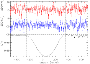
(a) $\xi$ Per LSD profile.

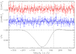
(b) $\alpha$ Cam LSD profile.

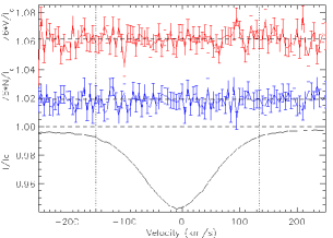
(c) HD 34656 LSD profile.

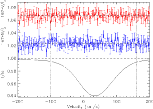
(d) $\lambda$ Ori A LSD profile.

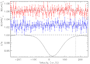
(e) $\epsilon$ Ori LSD profile.

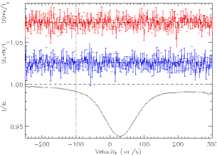
(f) 15 Mon LSD profile.

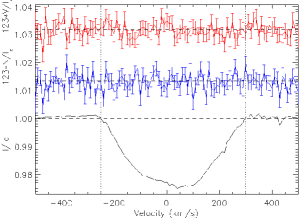
(g) HD 64760 LSD profile.

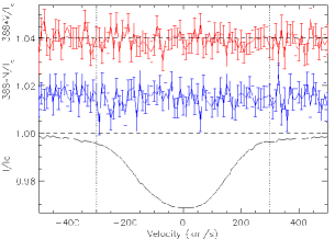
(h) $\zeta$ Pup LSD profile.

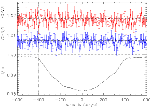
(i) $\zeta$ Oph LSD profile.

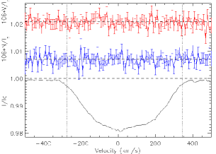
(j) 68 Cyg LSD profile.

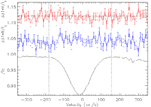
(k) 19 Cep LSD profile.

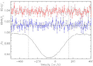
(l) $\lambda$ Cep LSD profile.

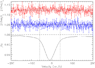
(m) 10 Lac LSD profile.

Figure 1: Typical LSD profiles for all stars in the sample. In each plot, the red line (top) is the Stokes V profile, while the blue line (middle) is a diagnostic null. Finally, the black line (bottom) is the Stokes I profile. The dotted lines represent the integration range for each star. We can see that no perceptible signal is found in any of the V profiles.

5 Magnetic field diagnosis

The LSD profiles were used to assess magnetic fields via two techniques: direct measurement diagnostics and Bayesian inference-based modeling.

5.1 Direct measurement diagnostics

Using the nightly-averaged profiles, as well as the individual ones, the disc-averaged longitudinal magnetic field ($B_{z}$) was computed using the first-order moments method (e.g. Wade et al. 2000). The integration ranges were chosen carefully, after a few trial calculations to determine how to minimize the error bars without losing any potential signal. Visually, the limits correspond loosely to the zero-points of the second derivative of the Stokes I profiles. Nightly longitudinal field measurements are listed in Table LABEL:tab:app. There are no significant detections. Not only do they seem normally distributed within the error bars, but these error bars are quite small in some cases and provided very tight constraints (e.g. 4 G error bar for 10 Lac on 17 October 2007). Furthermore, the longitudinal fields are also measured using the diagnostic nulls as a sanity check. On any given night, the error bars for the longitudinal fields measured from the V profile are consistent with those measured from the nulls, and the distributions of $B_{z}/\sigma_{B_{z}}$ obtained from each profile are essentially identical, which suggests that the V profile does not contain any more signal than the diagnostic nulls.

$\chi^{2}$ diagnostics are also performed by comparing both the V profile and the diagnostic null to the null hypothesis ($B=0$, therefore $V=0$ and $N=0$), and detection probabilities are derived from these values (Donati et al., 1997). These calculations are performed both within the LSD profile, as well as in the continuum. A detection probability below 99.9% is considered as a non-detection, a marginal detection possesses a detection probability between 99.9% and 99.999% and a definite detection has a detection probability of over 99.999% (for a discussion of these thresholds, see Donati et al. 1997). The 400+ individual and nightly-averaged V profiles are all non-detections, except 5 cases within the profile (1 in $\zeta$ Oph, 3 in 19 Cep and 1 in 10 Lac) and 1 in the continuum (in $\xi$ Per) all 6 of which are marginal detections. For the ones inside the line, except for a nightly-averaged observation in 10 Lac, the other 4 occurrences appear in individual observations, with a lower SNR. This could be due to somewhat noisier profiles, and since they are relatively isolated cases (for all 3 stars there are many more observations which are all non-detections), they are not perceived as being significant. As for the continuum marginal detection, it is also from a single observation and could be due to noise, as well as slight telluric contamination. On the whole, these results are largely consistent with those for the diagnostic nulls, further suggesting that there are no real detections.

In summary, both of these direct measurement diagnostics lead to the same conclusion, i.e. that no magnetic field is observed in any of these stars.

5.2 Bayesian inference

Additionally, to increase the SNR it is also possible to take advantage of the time resolution provided by repeated measurements. Indeed, taking into account the oblique dipole rotator model (Stibbs, 1950), data taken at different times should allow to view the surface magnetic field from different perspectives, thus lifting some of the degeneracy associated with the geometric parameters of the magnetic field, should it exist. Therefore, using the technique developed by Petit & Wade (2012), a fully self-consistent Bayesian inference method compares the observed profiles in the Stokes V and N parameters to synthetic Zeeman profiles for a grid of field strength and geometry parameters. The rotational phase of the observations is also allowed to vary freely, since rotational periods are unknown.

In order to produce synthetic Zeeman profiles to be used for this Bayesian technique, it is necessary to estimate the value of the projected rotational velocity of each star, as well as its macroturbulent velocity. These values are sometimes degenerate and difficult to determine with great precision. Instead of using previously published values, new values of $v\sin i$ were measured for all stars using the Fourier transform method (e.g. Simón-Díaz & Herrero 2007; Gray 1976). To this effect, synthetic spectra were computed with synth3 (Kochukhov, 2007), and the Oii $\lambda 4367$, Oiii $\lambda 5508$, Oiii $\lambda 5592$ and Civ $\lambda 5801$ lines were used to compare them to the data. In most cases (10/13), we get relatively (e.g. 20%) lower values of projected rotational velocity than those reported in the literature (Howarth et al., 1997), while for the 4 remaining stars, we get comparable or slightly higher results. This can be expected, since the line broadening is no longer solely attributed to rotation with this method.

Once the value of $v\sin i$ was determined, the LSD profiles (rather than individual lines, since these are the data we are looking to model) were then compared to synthetic Voigt profiles to refine the value of $v\sin i$ and determine $v_{mac}$. Because this process involved some level of degeneracy, the uncertainty on the obtained values could not be determined in a systematic way, but it is conservatively estimated to be about 10-20%. While this may seem large, tests using different pairs of values ($v\sin i$ and the associated $v_{mac}$) indicate that such a precision is quite sufficient, as errors of this magnitude do not significantly affect the results of the Bayesian analysis. A summary of these velocity measurements is given in Table 2, which also contains other relevant physical parameters. The macroturbulent velocities are likely to be systematically overestimated; the extra broadening from the helium lines behaves in a way similar to macroturbulence. However once again, extensive testing on our data has shown that this overestimation does not significantly alter the results of the Bayesian inference.

Ultimately, we modeled the observed I, V and N profiles to obtain probability density functions (PDFs) for 3 variables: the dipolar field strength ($B_{d}$), the inclination angle of the rotational axis ($i$) and the obliquity angle between the magnetic field axis and the rotational axis ($\beta$). It is also possible to marginalize the PDFs for each variable individually. However, it should be noted that the latter two geometric parameters cannot be constrained in the case of non-detections (Petit & Wade, 2012). Figure 2 shows the marginalized PDFs for three representative stars as a function of $B_{d}$. We can see that for each star, the PDF peaks at a value of 0, which is consistent with a non-detection. Additionally, a similar analysis was performed on the diagnostic null, with consistent results. Therefore, we obtained no information about the putative field’s geometry: we consider the only parameter of interest for this study to be the strength of the dipolar field. Since we only have non-detections, we can place upper limits on the dipolar field strength by using the 95.4% confidence region upper boundaries (which corresponds to the limit over which we expect the field to be detected, Petit & Wade 2012). These upper limits (noted as $B_{d,\textrm{max}}$) are listed in Table 2 (as well as the 68.3% confidence level upper limits for comparison purposes). The highest upper limit (95.4% interval) that we derive is that of HD 34656 (359 G). This is expected, since there was only a single observation for that star, therefore a lower SNR. The tail of the PDF falls off less abruptly as well (see Fig. 2), since statistically speaking, the observation could correspond to a particular phase where the field configuration is not suitable for detection. It should be remembered that this technique aims to take advantage of timeseries of LSD profiles; hence better constraints and a more peaked PDF could be obtained for this star with higher SNR observations and more extensive time coverage. All the other stars with upper limits over 100 G (5) have very high projected rotational velocities, which explains their poorer constraints. However, for the rest of the stars (7), we get extremely tight constraints, in particular in the case of 10 Lac (23 G). These values represent by far the tightest constraints ever obtained for any sample of OB stars (see Fig. 3 for a histogram of these upper limits).

However, even though fast rotating stars have poorer constraints on the strength of their hypothetical dipolar field, their rotation itself suggests that they do not possess such a field (or if so, a weak one). Indeed, a majority of magnetic OB stars are slow rotators. Moreover, all effectively single magnetic O stars are very slow rotators, with periods ranging from about one week to decades (e.g. Petit et al. 2013). This slow rotation is thought to be achieved by the magnetic field, which contributes to remove angular momentum from a star. This characteristic does not apply to our sample, in which nearly half (6/13) of the stars have projected rotational velocities of over 200 km/s. We can calculate a typical spindown timescale for a given magnetic field strength (see Eq. 8 of ud-Doula, Owocki & Townsend 2009). For example, if we perform that calculation on the supergiant HD 64760 using the 95.4% interval upper limit on the strength of the field, we get a spindown timescale of just under a million years, which seems incompatible with its projected rotational velocity of 250 km/s.

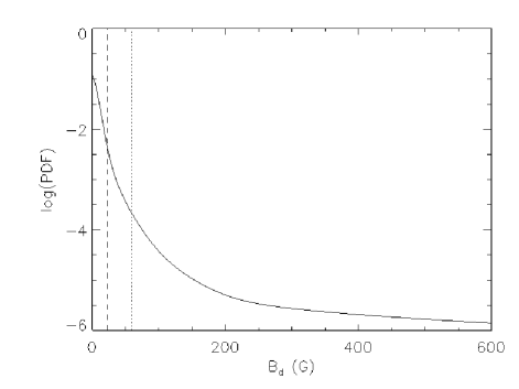
(a) $B_{d}$ PDF for 10 Lac.

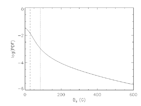
(b) $B_{d}$ PDF for $\alpha$ Cam.

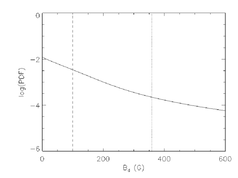
(c) $B_{d}$ PDF for HD 34656.

Figure 2: Logarithm of the probability density functions of the dipolar field strength ($B_{d}$) for three representative stars (10 Lac with the best constraints at the top, $\alpha$ Cam with typical constraints in the middle, and HD34656 with the worst constraints at the bottom) as derived from the Bayesian inference technique. For each plot, the dashed line delimits the 68.3% confidence interval, while the dotted line delimits the 95.4% confidence interval.

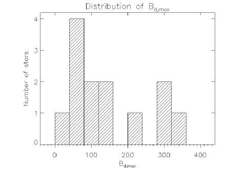
Figure 3: Histogram of the $B_{d,\textrm{max}}$ (95.4% interval upper limit) values derived from the Bayesian analysis (Table 2). Most stars have an upper limit below 120 G.

Another output of the Bayesian analysis is the odds ratio. This value represents the ratio of the likelihoods of each of the two hypotheses to be evaluated: $H_{0}$, corresponding to no magnetic field, and $H_{1}$, corresponding to a globally organized dipolar magnetic field. According to Jeffreys (1998), we would need an odds ratio below 1/3 to say that there is weak evidence in favour of the magnetic hypothesis. This ratio has been computed for each star (for the individual nightly observations, as well as for the entire dataset of a given star). For all V profiles, we get $odds(H_{0}/H_{1})>1$, except for two nightly profiles (1 for $\epsilon$ Ori and 1 for $\xi$ Per), but they do not go under 0.68. Typical values for the joint datasets range between 1 and 10. None of the stars yield odds ratios favouring the magnetic hypothesis. These results are also consistent with the odds ratios obtained from the null spectra.

It should be noted that this approach relies on a certain stability of the field. In particular, the geometry and strength of the dipole cannot undergo significant changes during the period of observation. On the other hand, this method is insensitive to any drift of the dipole in phase (e.g. precession of the magnetic axis around the rotation axis at a non-uniform rate). We assume that the geometry of the field remains stable over timescales of at least a few years given the temporal baseline of our observations; this assumption is found to be justified in intermediate-mass and massive stars (e.g. Wade et al. 2011; Grunhut 2012; Silvester, Kochukhov & Wade 2014). In any case, for a majority of stars in the sample, most observations are grouped within a few months, periods over which secular changes in the field geometry would not be important.

Once again, this analysis supports the view that no magnetic fields are observed, but further allows us to compute quantitative upper limits on the surface dipole component, necessary for evaluating the potential influence on the stellar wind.

Table 2: Stellar and magnetic parameters of the stars in the sample. Terminal wind velocities are obtained from Howarth et al. (1997) and references therein, as well as the previously published values of the projected rotational velocity (in parentheses). New values of $v\sin i$ obtained from the Fourier transform method (and refined by fitting the profiles) are reported as well. Nine stars of the sample are studied by Kaper et al. (1996) (a) and Kaper et al. (1997) (b), and all their other properties were obtained from these references (in particular, mass-loss rates are obtained using the empirical relation of Lamers & Leitherer 1993). For the B supergiants ($\epsilon$ Ori and HD 64760), Searle et al. (2008) (c) provide the radii and mass-loss rates, while the remaining parameters are obtained from Prinja, Massa & Fullerton (2002) (d). Finally, Lamers & Leitherer (1993) (e) provide the radii, mass-loss rates and effective temperatures of $\zeta$ Pup and $\zeta$ Oph; Howarth, Prinja & Massa (1995) (f) detail the DAC recurrence for the former and Howarth et al. (1993) (g) do the same for the latter.

Name	$R_{*}$	$T_{\mathrm{eff}}$	$\dot{M}$	$v_{\infty}$	$v\sin i$	$v_{mac}$	$P_{\mathrm{max}}$	$t_{\mathrm{DAC}}$	$B_{d,\textrm{max}}$	$B_{d,68.3\%}$	$\eta_{*,\textrm{max}}$	Ref.
	($R_{\odot}$)	(kK)	($M_{\odot}$/yr)	(km/s)	(km/s)	(km/s)	(d)	(d)	(G)	(G)
$\xi$ Per	11	36.0	$3\cdot 10^{-7}$	2330	215 (213)	80	2.6	2.0	59	22	0.11	a
$\alpha$ Cam	22	29.9	$9\cdot 10^{-7}$	1590	90 (129)	85	12.4	a few	85	28	0.48	a, b
HD 34656	10	36.8	$2\cdot 10^{-7}$	2155	70 (91)	65	7.2	0.9	359	100	5.75	a
$\lambda$ Ori A	12	35.0	$3\cdot 10^{-7}$	2175	55 (74)	60	11.0	$>$ 5	65	22	0.18	a
$\epsilon$ Ori	32	28.6	$2\cdot 10^{-6}$	1910	65 (91)	55	24.9	0.7	78	29	0.31	c, d
15 Mon	10	41.0	$4\cdot 10^{-7}$	2110	50 (67)	53	10.1	$>$ 4.5	84	30	0.16	a
HD 64760	23	23.1	$1\cdot 10^{-6}$	1500	250 (216)	50	4.7	a few	282	89	5.37	c, d
$\zeta$ Pup	16	42.4	$1\cdot 10^{-6}$	2485	220 (219)	80	3.7	0.8	121	34	0.29	e, f
$\zeta$ Oph	8	35.9	$9\cdot 10^{-8}$	1505	375 (372)	50	1.1	0.8	224	75	4.57	e, g
68 Cyg	14	36.0	$7\cdot 10^{-7}$	2340	290 (305)	65	2.4	1.3	286	90	1.86	a
19 Cep	18	30.2	$6\cdot 10^{-7}$	2010	56 (95)	70	16.3	$\sim$ 5	75	28	0.30	a
$\lambda$ Cep	17	42.0	$3\cdot 10^{-6}$	2300	200 (219)	80	4.3	1.4	136	50	0.15	a
10 Lac	9	38.0	$1\cdot 10^{-7}$	1140	21 (35)	30	21.7	$>$ 5	23	8	0.07	a

6 Notes on individual stars

The following subsections contain notes about each individual star.

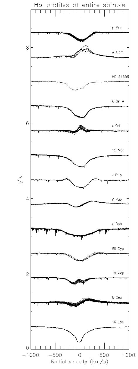
Figure 4: H$\alpha$ profiles of all stars (offset for viewing purposes). Some stars have very little to no variability, whereas others have significant variability (variable depths, emission, etc.).

6.1 $\xi$ Per

$\xi$ Per is a well-known O7.5 giant runaway star (Blaauw, 1992) whose DAC behaviour has been extensively studied in the past (e.g. Kaper et al. 1996). de Jong et al. (2001) have studied its spectral variability in a number of wind-sensitive lines and also confirm the presence of NRPs. While its high projected rotational velocity makes it harder to perform precise magnetometry, the excellent time coverage of this dataset leads to a very tight upper limit on the strength of an hypothetical dipolar field. There does not seem to be significant variation in the shape of H$\alpha$ during our observing runs, but rather simply a modulation of the depth of the line (see Fig. 4 for a summary of the H$\alpha$ profiles of all stars). Forty-four independent observations of $\xi$ Per were acquired over 13 nights in December 2006, September 2007 and November 2011. The smallest nightly longitudinal field error bar calculated from these data is 21 G, and the derived dipolar field strength upper limit is 59 G.

6.2 $\alpha$ Cam

Also a runaway (Blaauw, 1992), $\alpha$ Cam (O9.5 supergiant) exhibits a subtler DAC behaviour (Kaper et al., 1997). The projected rotational velocity was significantly revised (see Table 2). The H$\alpha$ profile undergoes important changes from night to night. Eleven independent observations of $\alpha$ Cam were acquired over 5 nights between 2006 and 2013. The smallest nightly longitudinal field error bar calculated from these data is 10 G, and the derived dipolar field strength upper limit is 85 G.

6.3 HD 34656

HD 34656 is a well-studied O7 bright giant (e.g. Fullerton, Gies & Bolton 1991, who observed line profile variations in its spectra) with relatively low $v\sin i$, making it an interesting target for this kind of study. Kaper et al. (1996) have characterized its DAC behaviour. Unfortunately, there was only a single observation of the star in the archive, therefore it was not possible to constrain its magnetic properties with great precision. The observation of HD 34656 was acquired in November 2011. The longitudinal field error bar calculated from this observation is 38 G, and the derived dipolar field strength upper limit is 359 G.

6.4 $\lambda$ Ori A

In a large separation double system with an early-B star (e.g. Scardia 1983), $\lambda$ Ori A is a slowly-rotating O8 giant, exhibiting well-known DAC behaviour (e.g. Kaper et al. 1996). We placed a very firm upper limit on its dipolar field strength. No detectable variations are found in H$\alpha$ in our observations. Twenty independent observations of $\lambda$ Ori A were acquired over 8 nights between 2007 and 2010. The smallest nightly longitudinal field error bar calculated from these data is 12 G, and the derived dipolar field strength upper limit is 65 G.

6.5 $\epsilon$ Ori

One of two B supergiants present in this sample, the DAC behaviour of $\epsilon$ Ori (B0) was first described by Prinja, Massa & Fullerton (2002). Evidence suggesting the possible presence of NRPs is offered by Prinja et al. (2004). We derive rather tight magnetic constraints, on top of observing significant variations of the H$\alpha$ profile over time. Seventy independent observations of $\epsilon$ Ori were acquired over 9 nights in October 2007, October 2008 and March 2009. The smallest nightly longitudinal field error bar calculated from these data is 6 G, and the derived dipolar field strength upper limit is 78 G.

6.6 15 Mon

A long period spectroscopic binary (Gies et al., 1997) with well-studied DACs (Kaper et al., 1996), 15 Mon (O7 dwarf) has low $v\sin i$, thus leading to a well-constrained field upper limit, even though it has not been observed as extensively as some other stars in this sample. Our observations of 15 Mon do not present noticeable changes in H$\alpha$. Contrarily to Hubrig et al. (2013), who claimed a 4.4 $\sigma$ detection based on two observations with FORS2 and SOFIN (longitudinal field error bars of 37-52 G), we do not find evidence supporting the presence of a large-scale dipolar magnetic field despite better quality data and more numerous observations. Indeed, sixteen independent observations of 15 Mon were acquired over 8 nights in December 2006, September-October 2007 and February 2012. The smallest nightly longitudinal field error bar calculated from these data is 20 G, and the derived dipolar field strength upper limit is 84 G.

6.7 HD 64760

This B0.5 supergiant was studied by Fullerton et al. (1997), who not only detect DACs, but also other forms of variability such as “phase bowing”, making this star a complex but very interesting case. It is also known to exhibit signs of NRPs (e.g. Kaufer, Prinja & Stahl 2002). However, due to its high projected rotational velocity, as well as the low number of observations, its magnetic properties are amongst the worst-constrained of this sample. There is no variation of H$\alpha$ between the two nights it was observed. Nine independent observations of HD 64760 were acquired over 2 nights in November 2010 and December 2012. The smallest nightly longitudinal field error bar calculated from these data is 37 G, and the derived dipolar field strength upper limit is 282 G.

6.8 $\zeta$ Pup

Characterized by a very strong wind, $\zeta$ Pup is a particularly hot O4 supergiant. Its DAC behaviour was evidenced by Howarth, Prinja & Massa (1995), while Reid & Howarth (1996) suggest the possibility of NRPs. We provide good limits on the magnetic field, albeit with a single night of observations. Better time coverage could provide much better constraints. It is not obvious from these data whether the H$\alpha$ profile varies over the course of the night. Thirty independent observations of $\zeta$ Pup were acquired over a single night in February 2012. The nightly longitudinal field error bar calculated from these data is 21 G, and the derived dipolar field strength upper limit is 121 G.

6.9 $\zeta$ Oph

A well-known runaway star (e.g. Perryman et al. 1997), $\zeta$ Oph (O9.5 dwarf) possesses a very high value of $v\sin i$ and short-period DACs (Howarth et al., 1993). Nonetheless, thanks to great time coverage, we obtain good magnetic constraints. Hubrig et al. (2013) claim this star to be magnetic, a result we do not reproduce here. Although their nightly observations possess better individual error bars, their longitudinal field curve has an amplitude of roughly 120 G and implies a surface dipole field of at least 360 G, which seems inconsistent with the 224 G upper limit we place on $B_{d}$. Period analysis performed on our longitudinal field measurements (for V and N) with period04 (Lenz & Breger, 2005) does not suggest periodic behaviour; in particular, the 0.8d and 1.3d periods reported by Hubrig et al. (2013) are not recovered. The periodogram of both the Stokes V and the null results are quite similar, further suggesting that no periodic signal is to be found. Individual Stokes I LSD profiles show strong line profile variations (LPV), in the form of bumps appearing and disappearing across the profile, which are indicative of the presence of NRPs, known to exist in this star (e.g. Walker et al. 2005). We do not detect noticeable variations in H$\alpha$ from night to night in our runs. Sixty-five independent observations of $\zeta$ Oph were acquired over 46 nights in 2011 and 2012. The smallest nightly longitudinal field error bar calculated from these data is 118 G, and the derived dipolar field strength upper limit is 224 G.

6.10 68 Cyg

The O7.5 runaway (e.g. Gies & Bolton 1986) giant 68 Cyg is a rapid rotator with well-studied DACs (Kaper et al., 1996). Factoring that in with a small number of observations, the putative dipolar magnetic field strength of 68 Cyg is not as well constrained as most of the other stars of the sample. However, H$\alpha$ is seen to be variable, though the pattern of its variation with time is not clear. Eight independent observations of 68 Cyg were acquired over 4 nights between 2006 and 2012. The smallest nightly longitudinal field error bar calculated from these data is 46 G, and the derived dipolar field strength upper limit is 286 G.

6.11 19 Cep

Believed to be a multiple star system (Mason et al., 1998), 19 Cep is known to exhibit DAC behaviour (Kaper et al., 1996) and has a primary (O9.5 supergiant) with low projected rotational velocity, so it was possible to obtain a firm upper limit on the dipolar magnetic field. The H$\alpha$ profiles show some signs of variability. Thirty-three independent observations of 19 Cep were acquired over 10 nights between 2006 and 2010. The smallest nightly longitudinal field error bar calculated from these data is 17 G, and the derived dipolar field strength upper limit is 75 G.

6.12 $\lambda$ Cep

The hot (O6) supergiant $\lambda$ Cep is a runaway (e.g. Gies & Bolton 1986) with a high value of $v\sin i$ and relatively short-period DACs (Kaper et al., 1996). Extensive time coverage leads to good magnetic constraints, despite the fast rotation. This star is also believed to harbour NRPs (e.g. de Jong et al. 1999). Strong variations of the H$\alpha$ profile are observed. Twenty-six independent observations of $\lambda$ Cep were acquired over 26 nights between 2006 and 2012. The smallest nightly longitudinal field error bar calculated from these data is 57 G, and the derived dipolar field strength upper limit is 136 G.

6.13 10 Lac

Hosting weaker (but detectable) wind variations (Kaper et al., 1996), 10 Lac is a sharp-lined O9 dwarf, leading to exceptionally tight limits on the field strength. No H$\alpha$ variations are detected in our data. Thirty-six independent observations of 10 Lac were acquired over 18 nights in December 2006, September-October-November 2007 and July 2008. The smallest nightly longitudinal field error bar calculated from these data is 4 G, and the derived dipolar field strength upper limit is 23 G, both of which are the best constraints obtained for any star in this sample.

7 Discussion and Conclusions

As shown in the previous sections, no large-scale dipolar magnetic field is detected in any of the 13 stars of this sample. However, in order to draw conclusions on whether such fields could be the cause for DACs, it is important to investigate the different possible interactions between weak, potentially undetected magnetic fields and stellar winds.

One form of interaction that has been increasingly investigated in the past years is magnetic wind confinement. Indeed, the magnetic field can channel the wind and closed loops can effectively “confine” it, leading to material trapped in a magnetosphere of closed magnetic loops. ud-Doula & Owocki (2002) introduce the following “wind confinement” parameter to characterize this interaction:

$$\eta_{*}=\frac{{B_{eq}}^{2}{R_{*}}^{2}}{\dot{M}v_{\infty}}$$ (1)

where $B_{eq}$ corresponds to the strength of the magnetic field at the equator (which equals half of the dipole polar field strength, $B_{d}$), $R_{*}$ is the stellar radius, $\dot{M}$ is the mass-loss rate and $v_{\infty}$ is the terminal velocity of the wind. In effect, this parameter corresponds to the ratio of the magnetic field energy density and the wind kinetic energy density at the stellar surface; therefore, its value gives a sense of which of the two dominates. If $\eta_{*}<<1$, then the wind’s momentum causes the magnetic field lines to stretch out radially and the outflow is essentially unperturbed. On the other hand, if $\eta_{*}>>1$, then the strong magnetic field lines are perpendicular to the outflow at the star’s magnetic equator, barring the passage of charged material. Depending on the rotational parameters of the star, this can lead either to a centrifugal or a dynamical magnetosphere (for a detailed description of both these cases, see Petit et al. 2013).

In intermediate cases however, the effect of the magnetic field can be somewhat more subtle. An in-depth analysis of this regime is presented by ud-Doula & Owocki (2002) and leads to two main thresholds:

• for $\eta_{*}>1$, the wind is considered to be confined by the magnetic field;

• for $0.1<\eta_{*}<1$, the wind is not confined, but its flow is significantly affected by the magnetic field.

Therefore, we will consider that for $\eta_{*}<0.1$, the dynamical effect of the magnetic field on the wind is likely to be too weak to cause DACs. An upper limit on the value of the $\eta_{*}$ parameter was computed for each star of the sample ($\eta_{*,\textrm{max}}$) using the upper limit on $B_{d}$ derived from the Bayesian inference, and the results are presented in Table 2.

It should be noted here that the wind parameter values used to compute these $\eta_{*}$ upper limits are determined empirically. For magnetic stars, it is necessary to use theoretical mass-loss rates instead of observed values to represent the net surface driving force, since a significant part of the outflow can be confined by the magnetic field, and would then not be detected at larger radii (Petit et al., 2013). However, in the case of apparently non-magnetic stars, the picture is not so clear. Furthermore, our empirical values are found to be systematically comparable to or smaller than theoretical values; since we are deriving conservative constraints, it seemed more consistent to use the overall smaller empirical values. Finally, while it might be argued that there are important uncertainties associated with empirical determinations of wind parameters, theoretical prescriptions (such as Vink, de Koter & Lamers 2001) propagate the rather sizeable uncertainties on masses and luminosities, so there is no obvious reason to choose one over the other based on such an argument.

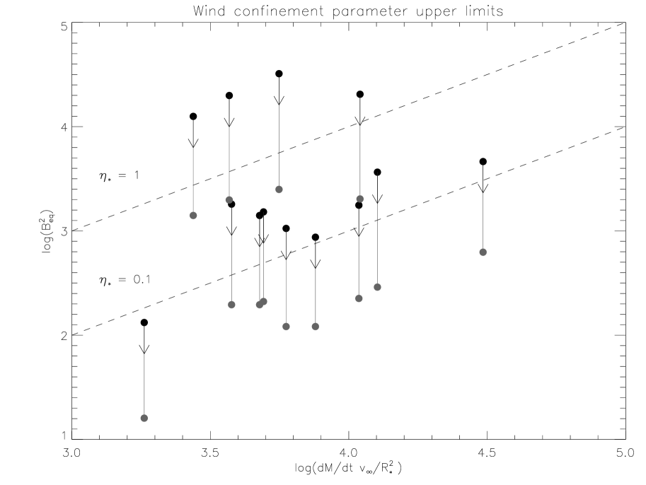
Figure 5: Comparison of the magnetic field energy density upper limits (vertical axis, 95.4% confidence interval upper limits indicated by black points, 68.3% confidence interval upper limits indicated by grey points) and the wind kinetic energy density values (horizontal axis) for all 13 stars of this study. Dashed lines show where $\eta_{*}=1$ and $\eta_{*}=0.1$. For most stars, the likelihood is greater than 95.4% that $\eta_{*}$ is below 1, and greater than 68.3% that it is below 0.1.

The value of $\eta_{*,\textrm{max}}$ ranges between 0.072 and 5.75, with one star below a value of 0.1 (10 Lac) and a majority of the stars below a value of 1 (9/13). As for the stars with $\eta_{*,\textrm{max}}>1$, they all have very high projected rotational velocities, thus making it difficult to tightly constrain the field strength. These results are also illustrated in Fig. 5, where the x-axis corresponds loosely to the wind kinetic energy density and the y-axis corresponds to the magnetic energy density. The dashed lines represent our two chosen thresholds. Given the fact that the represented values all correspond to upper limits, we can infer that at least a few of these stars do not have magnetic fields strong enough to dynamically affect the wind outflow on the equatorial plane (as also evidenced by the 68.3% confidence interval upper limits).

In addition to the upper limits, we use the PDFs to assess the sample’s distribution of confinement, assuming that each star contributes probabilistically to various field strength bins according to its normalized probability density function (constructing, in other words, a “probabilistic histogram” of field strengths). In this way, we account for both the most probable field strength as well as the large-field tail of the distributions. The top panel of Figure 6 shows this global cumulative PDF for the wind confinement parameter. We expect any star selected from the sample to have $\eta_{*}<0.02$ (which is well below the threshold of $\eta_{*}=0.1$) with a probability of 50%, or in other words, we expect half of the sample to have a confinement parameter value below 0.02. Using this cumulative PDF, we can also calculate that 75.6% of the sample should have $\eta_{*}<0.1$ and 93.9% of the sample should have $\eta_{*}<1$. Assuming this small sample is representative of the larger population of stars displaying DACs, this implies that there is no significant dipolar magnetic dynamic influence on the wind for most of these stars. Under these conditions, wind confinement by a dipolar magnetic field does not seem to be a viable mechanism to produce DAC-like variations in all stars.

The derived values of $\eta_{*}$ are sensitive to uncertainties in the values of $R_{*}$, $\dot{M}$ and $v_{\infty}$. While the last parameter is essentially identical in all studies, in some extreme cases values of $R_{*}$ can be up to 2-2.5 times larger than the adopted values, whereas $\dot{M}$ can be up to 10 times larger. Such differences would result respectively in a 6-fold increase and a 10-fold decrease in the inferred value of $\eta_{*}$. However, studies that infer larger stellar radii also tend to infer larger mass loss rates (e.g. Markova et al. 2004, with $\xi$ Per and HD 34656). Thus one effect approximately offsets the other. The largest potential increase in inferred $\eta_{*}$ for a star of our sample would occur for $\alpha$ Cam; based on the values measured by Najarro, Hanson & Puls (2011) (about 1.5 times increase in radius, and half the mass-loss rate), we obtain an increase of $\eta_{*}$ by a factor of 4. However, for typical combinations of $R_{*}$ and $\dot{M}$ obtained from other studies, we obtain values of $\eta_{*}$ that are either comparable in magnitude, or smaller (up to an order of magnitude) than those inferred using the adopted parameters.

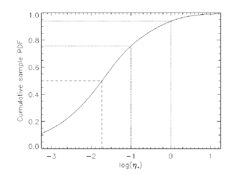
(a) $\eta_{*}$ cumulative PDF.

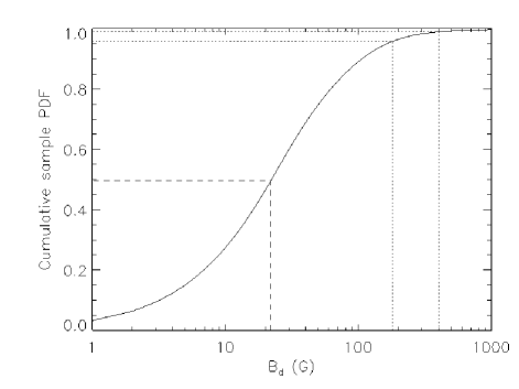
(b) $B_{d}$ cumulative PDF.

Figure 6: Cumulative PDFs of the total sample for $\eta_{*}$ (top) and $B_{d}$ (bottom). In both cases, the dashed line shows the 50% confidence interval upper limit. For the top panel the dotted lines represent, from left to right, $\eta_{*}=0.1$ and $\eta_{*}=1$. For the bottom panel the dotted lines represent, from left to right, the field strength required to produce a 10% and a 50% brightness enhancement (resp. about 180 G and 400 G).

Do these results rule out dipolar fields altogether? Cranmer & Owocki (1996) simply introduce bright spots on the surface of the star, with no particular attention to the mechanism creating these. While wind confinement is possibly the most obvious effect of a magnetic field on the ouflowing material driven from the surface of a massive star, there might also be more subtle interactions. For instance, the magnetic pressure at the poles of a weak large-scale dipolar field could lower the local gas pressure, thus reducing the gas density and leading to a lower optical depth. Hence, light coming from the pole would actually probe hotter regions within the star. This could cause bright spots like those in the Cranmer & Owocki (1996) model. Making a few assumptions (closely modeled on the calculations of Sundqvist et al. 2013), we can derive a simplified formula for the magnetic field ($B$) required to produce a given brightness enhancement. Indeed, if we consider a flux tube at the photosphere, we can compare a zone outside of the tube ($B=0$) to a zone inside the tube ($B=B_{\textrm{T}}$). Furthermore, we assume a grey atmosphere:

$$T(\tau)=T_{\textrm{eff}}\left(\frac{3}{4}\tau+\frac{1}{2}\right)^{\frac{1}{4}}$$ (2)

where $T$ is the temperature and $T_{\textrm{eff}}$ is the effective temperature (corresponding to an optical depth, $\tau$, of 2/3). At equilibrium, the gas pressures ($P_{\textrm{g}}$) inside and outside the tube only differ by the value of the magnetic pressure ($P_{\textrm{B}}=\frac{B^{2}}{8\pi}$):

$$P_{\textrm{g}}(r)=P_{\textrm{g}}^{\prime}(r)+P_{\textrm{B}}$$ (3)

where primed variables refer to values inside the flux tube, by opposition to unprimed variables which refer to values outside the flux tube. The optical depth can be written as a function of gas pressure:

$$\tau=\frac{\kappa P_{\textrm{g}}}{g}$$ (4)

where $\kappa$ is the mean Rosseland opacity, and $g$ is the surface gravity. To determine the brightness enhancement, we need to find the temperature corresponding to an optical depth of 2/3 inside the flux tube (assuming magneto-hydrostatic and temperature equilibrium at a given vertical depth):

$$T(\tau^{\prime}=2/3)=T_{\textrm{eff}}\left(1+\frac{3\kappa B^{2}}{32\pi g}\right)^{\frac{1}{4}}$$ (5)

Finally, since the flux is proportional to the fourth power of the temperature, the brightness enhancement can be expressed as:

$$\frac{F^{\prime}}{F}=1+\frac{3\kappa B^{2}}{32\pi g}$$ (6)

Now, using typical values for O dwarfs ($\kappa\sim 1$ and $\log g=4.0$), it is very simple to perform sample calculations. For instance, the main model used by Cranmer & Owocki (1996) uses a 50% enhancement. The field required to produce such an enhancement is of the order of 400 G, assuming a magnetic region surrounded by an adjacent non-magnetic region. On the other hand, the same paper shows that DAC-like behaviour can arise with an enhancement as small as 10%. The associated field would be of the order of 180 G. The dipolar field upper limits shown in Table 2 are almost all (9/13) under that value. While models with smaller brightness enhancements are not tested in their study, this mechanism associated with dipolar magnetic fields does not provide a viable way of producing DACs given the observational constraints obtained in this study.

Once again, in very much the same way as we did for $\eta_{*}$, we can compile a global cumulative PDF for $B_{d}$ (bottom panel of Figure 6). The results are quite telling: 50% of the sample should have $B_{d}<$ 23 G, and 95.8% (99.0%) of the sample should have a smaller dipolar field strength value than that required to produce a 10% (50%) local brightness enhancement.

Even if dipolar fields seem to be an unlikely cause for DACs, the general case for magnetism is not settled. Indeed, structured small-scale magnetic fields could arise as a consequence of the subsurface convection zone caused by the iron opacity bump at $T\simeq 150\textrm{kK}$ (Cantiello & Braithwaite, 2011). Then, magnetic spots at the surface of the star could possibly give rise to CIRs (e.g. Henrichs & Sudnik 2013), even though they are expected to be relatively weak (to have a surface field of at least 160 G, we need a 40+ $M_{\odot}$ star). While the detection of such fields is an arduous task (Kochukhov & Sudnik, 2013), proving their existence and understanding their structure might hold the key to this old problem, as well as other similar problems (e.g. in BA supergiants, see Shultz et al. 2013). Good candidates for follow-up deep magnetometry might be $\epsilon$ Ori and 10 Lac. The former has the advantage of being very bright and having a relatively low value of $v\sin i$, while the latter has very low projected rotational velocity (for an O star). 10 Lac already has decent time coverage, but could benefit from obtaining more observations per night.

In parallel to observational efforts, theoretical investigations are required in order to probe the parameter space of magnetic field strengths and configurations to find out which types of fields can give rise to DAC-like phenomena. Numerical simulations can also be used to investigate mechanisms other than magnetism, as well as constrain the required brightness enhancement in a Cranmer & Owocki (1996) model analog to create CIRs in the first place.

The next paper of this series will explore the magnetic spot hypothesis and hopefully place constraints on how likely such a mechanism is to cause DACs.

Appendix A List of observations

Table 3: Full list of nightly observations for each star. The date is given in universal time (UT), $B_{z}$ is the nightly measured longitudinal magnetic field value, ${\sigma}_{B_{z}}$ is the nightly error bar on the longitudinal field, $N_{\textrm{obs}}$ is the number of observations and the last column indicates whether they were obtained with ESPaDOnS (E) or NARVAL (N).

Name	Night	$B_{z}$	${\sigma}_{B_{z}}$	$N_{\textrm{obs}}$	E/N
		(G)	(G)
$\xi$ Per	10 Dec. 2006	19	41	3	N
$\xi$ Per	13 Dec. 2006	-10	36	3	N
$\xi$ Per	14 Dec. 2006	49	42	3	N
$\xi$ Per	15 Dec. 2006	28	22	7	N
$\xi$ Per	16 Dec. 2006	-25	138	1	N
$\xi$ Per	06 Sep. 2007	5	25	7	N
$\xi$ Per	07 Sep. 2007	-10	21	6	N
$\xi$ Per	08 Sep. 2007	-20	26	4	N
$\xi$ Per	09 Sep. 2007	32	48	2	N
$\xi$ Per	10 Sep. 2007	59	55	1	N
$\xi$ Per	11 Sep. 2007	46	61	1	N
$\xi$ Per	12 Sep. 2007	41	70	1	N
$\xi$ Per	01 Nov. 2011	-15	48	5	E
$\alpha$ Cam	13 Dec. 2006	64	35	1	N
$\alpha$ Cam	21 Dec. 2007	2	10	4	E
$\alpha$ Cam	14 Nov. 2010	11	20	2	E
$\alpha$ Cam	31 Dec. 2012	6	24	1	E
$\alpha$ Cam	01 Jan. 2013	11	25	3	E
HD 34656	11 Nov. 2011	-35	38	1	E
$\lambda$ Ori A	21 Dec. 2007	-15	23	2	E
$\lambda$ Ori A	18 Jan. 2008	36	46	1	E
$\lambda$ Ori A	22 Jan. 2008	-14	22	2	E
$\lambda$ Ori A	14 Oct. 2008	31	33	2	N
$\lambda$ Ori A	26 Oct. 2008	17	15	7	N
$\lambda$ Ori A	15 Mar. 2009	17	30	1	N
$\lambda$ Ori A	17 Mar. 2009	12	25	1	N
$\lambda$ Ori A	16 Oct. 2010	-2	12	4	E
$\epsilon$ Ori	15 Oct. 2007	44	75	1	N
$\epsilon$ Ori	17 Oct. 2007	-34	29	6	N
$\epsilon$ Ori	18 Oct. 2007	-3	6	28	N
$\epsilon$ Ori	21 Oct. 2007	2	10	8	N
$\epsilon$ Ori	24 Oct. 2007	17	13	6	N
$\epsilon$ Ori	13 Oct. 2008	20	9	9	E
$\epsilon$ Ori	25 Oct. 2008	-2	13	10	N
$\epsilon$ Ori	15 Mar. 2009	26	35	1	N
$\epsilon$ Ori	16 Mar. 2009	4	25	1	N
15 Mon	10 Dec. 2006	-9	50	1	N
15 Mon	15 Dec. 2006	-3	27	1	N
15 Mon	09 Sep. 2007	-17	39	1	N
15 Mon	10 Sep. 2007	-1	30	1	N
15 Mon	11 Sep. 2007	-22	44	1	N
15 Mon	20 Oct. 2007	-2	26	4	N
15 Mon	23 Oct. 2007	16	24	4	N
15 Mon	03 Feb. 2012	0	20	3	E
HD 64760	21 Nov. 2010	51	37	6	E
HD 64760	31 Dec. 2012	15	59	3	E
$\zeta$ Pup	14 Feb. 2012	-12	21	30	E
$\zeta$ Oph	18 Mar. 2011	92	438	1	N
$\zeta$ Oph	21 Mar. 2011	-336	361	1	N
$\zeta$ Oph	05 Apr. 2011	-266	406	1	N
$\zeta$ Oph	08 Jun. 2011	-134	118	20	E
$\zeta$ Oph	10 Jun. 2011	417	423	1	N
$\zeta$ Oph	13 Jun. 2011	-261	426	1	N
$\zeta$ Oph	14 Jun. 2011	34	310	1	N
$\zeta$ Oph	15 Jun. 2011	106	377	1	N
$\zeta$ Oph	04 Jul. 2011	-206	302	1	N
$\zeta$ Oph	07 Jul. 2011	127	411	1	N
$\zeta$ Oph	10 Jul. 2011	170	342	1	N
$\zeta$ Oph	11 Jul. 2011	-51	320	1	N
$\zeta$ Oph	10 Aug. 2011	-9	315	1	N
$\zeta$ Oph	11 Aug. 2011	120	345	1	N
$\zeta$ Oph	15 Aug. 2011	242	374	1	N
$\zeta$ Oph	16 Aug. 2011	174	335	1	N
$\zeta$ Oph	17 Aug. 2011	-85	349	1	N
$\zeta$ Oph	18 Aug. 2011	-77	579	1	N
$\zeta$ Oph	20 Aug. 2011	-82	418	1	N
$\zeta$ Oph	21 Aug. 2011	-91	297	1	N
$\zeta$ Oph	22 Aug. 2011	108	499	1	N
$\zeta$ Oph	23 Aug. 2011	14	295	1	N
$\zeta$ Oph	26 Aug. 2011	455	685	1	N
$\zeta$ Oph	27 Aug. 2011	-277	524	1	N
$\zeta$ Oph	28 Aug. 2011	769	840	1	N
$\zeta$ Oph	16 Jan. 2012	-476	446	1	N
$\zeta$ Oph	17 Jan. 2012	-444	383	1	N
$\zeta$ Oph	24 Jan. 2012	-52	317	1	N
$\zeta$ Oph	25 Jan. 2012	41	282	1	N
$\zeta$ Oph	27 Jan. 2012	-126	596	1	N
$\zeta$ Oph	21 Jun. 2012	39	351	1	N
$\zeta$ Oph	22 Jun. 2012	185	316	1	N
$\zeta$ Oph	23 Jun. 2012	380	298	1	N
$\zeta$ Oph	09 Jul. 2012	409	348	1	N
$\zeta$ Oph	12 Jul. 2012	152	369	1	N
$\zeta$ Oph	06 Aug. 2012	-132	321	1	N
$\zeta$ Oph	07 Aug. 2012	75	382	1	N
$\zeta$ Oph	08 Aug. 2012	-248	335	1	N
$\zeta$ Oph	09 Aug. 2012	171	413	1	N
$\zeta$ Oph	12 Aug. 2012	-171	491	1	N
$\zeta$ Oph	14 Aug. 2012	462	361	1	N
$\zeta$ Oph	16 Aug. 2012	-161	474	1	N
$\zeta$ Oph	17 Aug. 2012	-143	413	1	N
$\zeta$ Oph	18 Aug. 2012	-572	448	1	N
$\zeta$ Oph	19 Aug. 2012	-178	403	1	N
$\zeta$ Oph	20 Aug. 2012	56	383	1	N
68 Cyg	16 Dec. 2006	131	479	1	N
68 Cyg	10 Sep. 2007	80	101	1	N
68 Cyg	12 Nov. 2007	-106	197	1	N
68 Cyg	29 Sep. 2012	-11	46	5	E
19 Cep	13 Dec. 2006	-20	44	1	N
19 Cep	09 Nov. 2007	9	59	1	N
19 Cep	13 Nov. 2007	-129	97	1	N
19 Cep	22 Dec. 2007	-8	22	3	E
19 Cep	21 Jun. 2008	-57	28	5	N
19 Cep	22 Jun. 2008	9	20	5	N
19 Cep	25 Jun. 2008	2	24	3	N
19 Cep	27 Jun. 2008	-18	17	5	N
19 Cep	28 Jun. 2008	-5	19	5	N
19 Cep	26 Jul. 2010	23	36	4	E
$\lambda$ Cep	13 Dec. 2006	64	79	1	N
$\lambda$ Cep	07 Jul. 2011	-100	63	1	N
$\lambda$ Cep	08 Jul. 2011	36	60	1	N
$\lambda$ Cep	10 Aug. 2011	-15	65	1	N
$\lambda$ Cep	27 Aug. 2011	-56	83	1	N
$\lambda$ Cep	28 Aug. 2011	-2	67	1	N
$\lambda$ Cep	16 Jun. 2012	4	95	1	N
$\lambda$ Cep	22 Jun. 2012	-64	68	1	N
$\lambda$ Cep	24 Jun. 2012	31	92	1	N
$\lambda$ Cep	09 Jul. 2012	-37	78	1	N
$\lambda$ Cep	18 Jul. 2012	38	63	1	N
$\lambda$ Cep	19 Jul. 2012	-9	66	1	N
$\lambda$ Cep	22 Jul. 2012	-20	67	1	N
$\lambda$ Cep	23 Jul. 2012	10	67	1	N
$\lambda$ Cep	24 Jul. 2012	7	62	1	N
$\lambda$ Cep	06 Aug. 2012	88	57	1	N
$\lambda$ Cep	07 Aug. 2012	-149	80	1	N
$\lambda$ Cep	08 Aug. 2012	53	67	1	N
$\lambda$ Cep	09 Aug. 2012	41	58	1	N
$\lambda$ Cep	11 Aug. 2012	-12	126	1	N
$\lambda$ Cep	12 Aug. 2012	85	103	1	N
$\lambda$ Cep	13 Aug. 2012	-66	65	1	N
$\lambda$ Cep	15 Aug. 2012	-11	97	1	N
$\lambda$ Cep	16 Aug. 2012	62	86	1	N
$\lambda$ Cep	17 Aug. 2012	-13	86	1	N
$\lambda$ Cep	18 Aug. 2012	173	149	1	N
10 Lac	10 Dec. 2006	-6	7	1	N
10 Lac	11 Dec. 2006	-1	7	1	N
10 Lac	13 Dec. 2006	8	8	1	N
10 Lac	14 Dec. 2006	-6	7	1	N
10 Lac	15 Dec. 2006	8	6	1	N
10 Lac	16 Dec. 2006	11	9	1	N
10 Lac	07 Sep. 2007	-2	6	1	N
10 Lac	15 Oct. 2007	9	6	3	N
10 Lac	16 Oct. 2007	12	6	3	N
10 Lac	17 Oct. 2007	1	4	3	N
10 Lac	18 Oct. 2007	-6	8	3	N
10 Lac	19 Oct. 2007	-6	4	3	N
10 Lac	20 Oct. 2007	1	4	3	N
10 Lac	21 Oct. 2007	5	5	3	N
10 Lac	23 Oct. 2007	2	5	3	N
10 Lac	24 Oct. 2007	-3	4	3	N
10 Lac	06 Nov. 2007	-14	14	1	N
10 Lac	26 Jul. 2008	9	10	1	E

References

- Blaauw (1992) Blaauw A., 1992, ASPC, 35, 207
- Bouret et al. (2012) Bouret J.C., Hillier D.J., Lanz T., Fullerton A.W., 2012, A&A, 544, 67
- Braithwaite & Nordlund (2006) Braithwaite J., Nordlund Å., 2006, A&A, 450, 1077
- Cantiello & Braithwaite (2011) Cantiello M., Braithwaite J., 2011, A&A, 534, A140
- Castor, Abbott & Klein (1975) Castor J.I., Abbott D.C., Klein R.I., 1975, ApJ, 195, 157
- Cranmer & Owocki (1996) Cranmer S.R., Owocki S.P., 1996, ApJ, 462, 469
- Cuntz & Stencel (1992) Cuntz M., Stencel R.E., 1992, ASPC, 26, 451
- de Jong et al. (1999) de Jong J.A., Henrichs H.F., Schrijvers C., Gies D.R., Telting J.H., Kaper L., Zwarthoed G.A.A., 1999, A&A, 345, 172
- de Jong et al. (2001) de Jong J.A., Henrichs H.F., Kaper L., Nichols J.S., Bjorkman K., Bohlender D.A., Cao H., Gordon K., Hill G., Jiang Y., Kolka I., Morrison N., Neff J., O’Neal D., Scheers B., Telting J.H., 2001, A&A, 368, 601
- Donati et al. (1997) Donati J.F., Semel M., Carter B.D., Rees D.E., Collier Cameron A., 1997, MNRAS, 291, 658
- Duez & Mathis (2010) Duez V., Mathis S., 2010, A&A, 517, 58
- Fullerton, Gies & Bolton (1991) Fullerton A.W., Gies D.R., Bolton C.T., 1991, ApJ, 368, L35
- Fullerton et al. (1997) Fullerton A.W., Massa D.L., Prinja R.K., Owocki S.P., Cranmer S.R., 1997, A&A, 327, 699
- Fullerton (2003) Fullerton A.W., 2003, ASPC, 305, 333
- Gies & Bolton (1986) Gies D.R., Bolton C.T., 1986, ApJS, 61, 419
- Gies et al. (1997) Gies D.R., Mason B.D., Bagnuolo W.G. Jr., Hahula M.E., Hartkopf W.I., McAlister H.A., Thaller M.L., McKibben W.P., Penny L.R., 1997, ApJ, 475, 49
- Gray (1976) Gray D.F., 1976, The observation and analysis of stellar photospheres, Wiley-Interscience, New York
- Grunhut (2012) Grunhut J.H., Wade G.A., Sundqvist J.O., ud-Doula A., Neiner C., Ignace R., Marcolino W.L.F., Rivinius T., Fullerton A., Kaper L., Mauclaire B., Buil C., Garrel T., Ribeiro J., Ubaud S., 2012, MNRAS, 426, 2208
- Henrichs & Sudnik (2013) Henrichs H.F., Sudnik N.P., 2013, arXiv, 1310, 5264
- Howarth & Prinja (1989) Howarth I.D., Prinja R.K., 1989, ApJS, 69, 527
- Howarth et al. (1993) Howarth I.D., Bolton C.T., Crowe R.A., Ebbets D.C., Fieldus M.S., Fullerton A.W., Gies D.R., McDavid D., Prinja R.K., Reid A.H.N., Shore S.N., Smith K.C., 1993, ApJ, 417, 338
- Howarth, Prinja & Massa (1995) Howarth I.D., Prinja R.K., Massa D., 1995, ApJ, 452, L65
- Howarth et al. (1997) Howarth I.D., Siebert K.W., Hussain G.A.J., Prinja R.K., 1997, MNRAS, 284, 265
- Hubrig et al. (2013) Hubrig S., Schöller M., Ilyin I., Kharchenko N.V., Oskinova L.M., Langer N., González J.F., Kholtygin A.F., Briquet M., MAGORI Collaboration, 2013, A&A, 551, A33
- Jeffreys (1998) Jeffreys H., 1998, Theory of Probability, 3rd edn., Oxford University Press, Oxford
- Kaper et al. (1996) Kaper L., Henrichs H.F., Nichols J.S., Snoek L.C., Volten H., Zwarthoed G.A.A., 1996, A&AS, 116, 257
- Kaper et al. (1997) Kaper L., Henrichs H.F., Fullerton A.W., Ando H., Bjorkman K.S., Gies D.R., Hirata R., Kambe E., McDavid D., Nichols J.S., 1997, A&A, 327, 281
- Kaufer, Prinja & Stahl (2002) Kaufer A., Prinja R.K., Stahl O., 2002, A&A, 382, 1032
- Kochukhov (2007) Kochukhov O., in Romanuyk I.I., Kudryavtsev D.O., eds., Physics of Magnetic Stars, SAO RAS, Nizhnij Arkhyz, p.109
- Kochukhov, Makaganiuk & Piskunov (2010) Kochukhov O., Makaganiuk V., Piskunov N., 2010, A&A, 524, A5
- Kochukhov & Sudnik (2013) Kochukhov O., Sudnik N., 2013, A&A, 554, A93
- Kupka et al. (2000) Kupka F.G., Ryabchikova T.A., Piskunov N.E., Stempels H.C., Weiss W.W., 2000, BaltA, 9, 590
- Lamers & Leitherer (1993) Lamers H.J.G.L.M., Leitherer C., 1993, ApJ, 412, 771
- Lenz & Breger (2005) Lenz P., Breger M., 2005, CoAst, 146, 53
- Lobel (2013) Lobel A., 2013, poster 43 in Massive Stars: From to , conference held in Rhodes, Greece, 10-14 June 2013
- Markova et al. (2004) Markova N., Puls J., Repolust T., Markov H., 2004, A&A, 413, 693
- Mason et al. (1998) Mason B.D., Gies D.R., Hartkopf W.I., Bagnuolo W.G. Jr., ten Brummelaar T., McAlister H.A., 1998, AJ, 115, 821
- Massa et al. (1995) Massa D., Fullerton A.W., Nichols J.S., Owocki S.P., Prinja R.K., St-Louis N., Willis A.J., Altner B., Bolton C.T., Cassinelli J.P., Cohen D., Cooper R.G., Feldmeier A., Gayley K.G., Harries T., Heap S.R., Henriksen R.N., Howarth I.D., Hubeny I., Kambe E., Kaper L., Koenigsberger G., Marchenko S., McCandliss S.R., Moffat A.F.J., Nugis T., Puls J., Robert C., Schulte-Ladbeck R.E., Smith L.J., Smith M.A., Waldron W.L., White R.L., 1995, ApJ, 452, L53
- Moffat et al. (1994) Moffat A.F.J., Lepine S., Henriksen R.N., Robert C., 1994, Ap&SS, 216, 55
- Mullan (1986) Mullan D.J., 1986, A&A, 165, 157
- Najarro, Hanson & Puls (2011) Najarro F., Hanson M.M., Puls J., 2011, A&A, 535, 32
- Perryman et al. (1997) Perryman M.A.C., Lindegren L., Kovalevsky J., Hoeg E., Bastian U., Bernacca P.L., Crézé M., Donati F., Grenon M., Grewing M., van Leeuwen F., van der Marel H., Mignard F., Murray C.A., Le Poole R.S., Schrijver H., Turon C., Arenou F., Froeschlé M., Petersen C.S., 1997, A&A, 323, L49
- Petit & Wade (2012) Petit V., Wade G.A., 2012, MNRAS, 420, 773
- Petit et al. (2013) Petit V., Owocki S.P., Wade G.A., Cohen D.H., Sundqvist J.O., Gagné M., Maíz Apellániz J., Oksala M.E., Bohlender D.A., Rivinius T., Henrichs H.F., Alecian E., Townsend R.H.D., ud-Doula A., MiMeS Collaboration, 2013, MNRAS, 429, 398
- Prinja (1988) Prinja R.K., 1988, MNRAS, 231, 21
- Prinja & Howarth (1986) Prinja R.K., Howarth I.D., 1986, ApJS, 61, 357
- Prinja, Massa & Fullerton (2002) Prinja R.K., Massa D., Fullerton A.W., 2002, A&A, 388, 587
- Prinja et al. (2004) Prinja R.K., Rivinius T., Stahl O., Kaufer A., Foing B.H., Cami J., Orlando S., 2004, A&A, 418, 727
- Reid & Howarth (1996) Reid A.H.N., Howarth I.D., 1996, A&A, 311, 616
- Scardia (1983) Scardia M., 1983, A&AS, 53, 433
- Searle et al. (2008) Searle S.C., Prinja R.K., Massa D., Ryans R., 2008, A&A, 481, 777
- Repolust, Puls & Herrero (2004) Repolust T., Puls J., Herrero A., 2004, A&A, 415, 349
- Shultz et al. (2013) Shultz M., Wade G.A., Petit V., Grunhut J., Neiner C., Hanes D., MiMeS Collaboration, 2013, arXiv, 1311, 5116
- Silvester, Kochukhov & Wade (2014) Silvester J., Kochukhov O., Wade G.A., 2014, MNRAS, 440, 182
- Simón-Díaz & Herrero (2007) Simón-Díaz S., Herrero A., 2007, A&A, 468, 1063
- Stibbs (1950) Stibbs D.W.N., 1950, MNRAS, 110, 395
- Sundqvist & Owocki (2013) Sundqvist J.O., Owocki S.P., 2013, MNRAS, 428, 1837
- Sundqvist et al. (2013) Sundqvist J.O., Petit V., Owocki S.P., Wade G.A., Puls J., MiMeS Collaboration, 2013, MNRAS, 433, 2497
- ud-Doula & Owocki (2002) ud-Doula A., Owocki S.P., 2002, ApJ, 576, 413
- ud-Doula, Owocki & Townsend (2009) ud-Doula A., Owocki S.P., Townsend R.H.D, 2009, MNRAS, 392, 1022
- Vink, de Koter & Lamers (2001) Vink J.S., de Koter A., Lamers H.J.G.L.M., 2001, A&A, 369, 574
- Wade et al. (2000) Wade G.A., Donati J.F., Landstreet J.D., Shorlin S.L.S., 2000, MNRAS, 313, 851
- Wade & the MiMeS Collaboration (2010) Wade G.A., MiMeS Collaboration, 2010, arXiv, 1012, 2925
- Wade et al. (2011) Wade G.A., Howarth I.D., Townsend R.H.D., Grunhut J.H., Shultz M., Bouret J.C., Fullerton A., Marcolino W., Martins F., Nazé Y., Ud Doula A., Walborn N.R., Donati J.F., 2011, MNRAS, 416, 3160
- Wade et al. (2013) Wade G.A., Grunhut J., Alecian E., Neiner C., Aurière M., Bohlender D.A., David-Uraz A., Folsom C., Henrichs H.F., Kochukhov O., Mathis S., Owocki S., Petit V., MiMeS Collaboration, 2013, arXiv, 1310, 3965
- Walker et al. (2005) Walker G.A.H., Kuschnig R., Matthews J.M., Reegen P., Kallinger T., Kambe E., Saio H., Harmanec P., Guenther D.B., Moffat A.F.J., Rucinski S.M., Sasselov D., Weiss W.W., Bohlender D.A., Božić H., Hashimoto O., Koubský P., Mann R., Ruždjak D., Škoda P., Šlechta M., Sudar D., Wolf M., Yang S., 2005, ApJ, 623, L145