Detection of solar-like oscillations in the bright red giant stars $\gamma$ Psc and $\theta^{1}$ Tau from a 190-day high-precision spectroscopic multisite campaign

Abstract

Context. Red giants are evolved stars which exhibit solar-like oscillations. Although a multitude of stars have been observed with space telescopes, only a handful of red-giant stars were targets of spectroscopic asteroseismic observing projects.

Aims. We search for solar-like oscillations in the two bright red-giant stars $\gamma$ Psc and $\theta^{1}$ Tau from time series of ground-based spectroscopy and determine the frequency of the excess of oscillation power $\nu_{\mathrm{max}}$ and the mean large frequency separation $\Delta\nu$ for both stars. Seismic constraints on the stellar mass and radius will provide robust input for stellar modelling.

Methods. The radial velocities of $\gamma$ Psc and $\theta^{1}$ Tau were monitored for 120 and 190 days, respectively. Nearly 9000 spectra were obtained. To reach the accurate radial velocities, we used simultaneous thorium-argon and iodine-cell calibration of our optical spectra. In addition to the spectroscopy, we acquired VLTI observations of $\gamma$ Psc for an independent estimate of the radius. Also 22 days of observations of $\theta^{1}$ Tau with the MOST-satellite were analysed.

Results. The frequency analysis of the radial velocity data of $\gamma$ Psc revealed an excess of oscillation power around 32 $\mu$Hz and a large frequency separation of 4.1$\pm$0.1 $\mu$Hz. $\theta^{1}$ Tau exhibits oscillation power around 90 $\mu$Hz, with a large frequency separation of 6.9$\pm$0.2 $\mu$Hz. Scaling relations indicate that $\gamma$ Psc is a star of about 1 M_⊙ and 10 R_⊙. $\theta^{1}$ Tau appears to be a massive star of about 2.7 M_⊙ and 10 R_⊙. The radial velocities of both stars were found to be modulated on time scales much longer than the oscillation periods.

Conclusions. The estimated radii from seismology are in agreement with interferometric observations and also with estimates based on photometric data. While the mass of $\theta^{1}$ Tau is in agreement with results from dynamical parallaxes, we find a lower mass for $\gamma$ Psc than what is given in the literature. The long periodic variability agrees with the expected time scales of rotational modulation.

1 Introduction

Table 1: Fundamental parameters and computed asteroseismic characteristics of the campaign targets.

Star	Sp.	RA	DE	V	$\pi$	$v\sin i$	Teff	[Fe/H]	Lum	Radius	Mass	$\nu_{\rm max}$	$\Delta\nu$	Prot
Name	Typ	[h m]	[∘ ’]	[mag]	[mas]	[km s-1]	[K]	[dex]	[L⊙]	[R⊙]	[M⊙]	[$\mu$Hz]	[$\mu$Hz]	[days]
$\gamma$ Psc	G9III	23 17	+03 17	3.7	23.6$\pm$0.2	4.7	4940	-0.62	63	10.4	1.87	60	5.7	112.6
$\theta^{1}$ Tau	K0III	04 29	+15 58	3.8	21.1$\pm$0.3	4.2	5000	+0.10	69	11.4	2.8$\pm$0.5	76	6.1	138.2

Table 2: Observatories participating in the campaign.

Instrument	Technique	Telescope	Location	Calibr.	R	N${}_{\gamma\,Psc}$	N${}_{\theta^{1}\,Tau}$	Spectra	Observer
Hermes	Spec.	1.2 m Mercator	La Palma/Spain	ThArNe	46000	1339	1329	2668	PGB, MH, SB, et al.
Coralie	Spec.	1.2 m Euler	La Silla/Chile	ThAr	62000	1949	792	2741	PGB, SS
Hides	Spec.	1.88 m telesc.	Okayama/Japan	Iodine	50000	1306	1284	2590	EK, AH, PGB
Sophie	Spec.	1.93 m telesc.	OHP/France	ThAr	75000	485	360	845	PM
Sarg	Spec.	3.58 m TNG	La Palma/Spain	Iodine	46000	-	-	-	RO
Amber	Interf.	VLTI	Paranal/Chile	-	30	-	-	-	SB

Solar-like oscillations are excited stochastically by motions in the convective envelope of stars. For low-mass stars, they are found in all evolutionary states, between the main sequence and horizontal branch of helium-core burning stars (e.g. Leighton et al., 1962; Frandsen et al., 2002; Carrier et al., 2003; Hekker et al., 2009; Chaplin et al., 2011; Huber et al., 2011; Kallinger et al., 2012; Mosser et al., 2013) and were even detected in the M5 super giant $\alpha$ Her (Moravveji et al., 2013). These very characteristic oscillations lead to a nearly regular spaced comb-like pattern in the power spectrum. It was shown by Deubner (1975) that this ridge structure is governed by the degree of oscillation modes and resembles the predictions made by Ando & Osaki (1975). Empirically, the frequency patterns of solar-like oscillations were described through scaling relations by Kjeldsen & Bedding (1995). Since then, these relations have been tested and revised from large sample studies based on high-precision space photometry of red giants in clusters and in eclipsing binaries besides single stars (e.g. Corsaro et al., 2012b; Frandsen et al., 2013; Kallinger et al., 2010, respectively). Indications of non-radial oscillation modes were found in the variations of the absorption lines of bright red giants (Hekker et al., 2006; Hekker & Aerts, 2010) but firmly established in a large set of red giants observed with the CoRoT satellite (De Ridder et al., 2009). The identification of dipole mixed modes extended the sensitivity of the seismic analyses also towards the core of evolved stars (Beck et al., 2011; Bedding et al., 2011; Mosser et al., 2011). The analysis of solar-like oscillations enabled us to unravel many open questions on stellar structure and evolution, such as constraining the internal rotational gradient (Elsworth et al., 1995; Beck et al., 2012; Deheuvels et al., 2012) or determining the evolutionary status in terms of nuclear burning of a given red-giant star (Bedding et al., 2011; Mosser et al., 2011).

Spectroscopic time series offer a different look at stars, as spectroscopy and photometry have different mode sensitivities because modes with an odd spherical degree $l$ exhibit a better visibility in spectroscopy than in photometry (Aerts et al., 2010). Radial velocity data is less effected by granulation noise, providing a wider frequency range that can be investigated (Aerts et al., 2010). In addition, most targets of space observations are faint. As typical target stars for spectroscopy are bright, they are well studied and many complimentary parameters are found in the literature. Furthermore, experience has shown that the long term stability is a major issue for space missions and it is very challenging to constrain weak signals on the order of several tens of days (e.g. Beck et al., 2014). With robust calibration techniques, we can also study variations on the order of more than 100 days and longer from stable spectrographs.

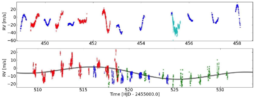
Figure 1: Example of radial velocity measurements of $\gamma$ Psc in September 2010 (top panel) and $\theta^{1}$ Tau in November 2010 (bottom panel). The data sets of Hermes, Hides, Coralie and Sophie are shown in red, blue, green, and cyan, respectively. The full data set is depicted in Fig.3. The radial velocities of $\theta^{1}$ Tau have been detrended for the binary orbit, shown in Fig. 4. The gray line indicates the 16.57 d modulation of the radial velocities, found in $\theta^{1}$ Tau.

Although space-photometry is available for stars in all phases on the red-giant branch, no spectroscopic time series have deliberately been obtained for stars in the red clump. Most campaigns concentrate on stars close to or on the main sequence, as the higher oscillation frequencies do not require extensive time series to resolve the variation. In this paper we describe the definition, data acquisition, and analysis of an extensive observational campaign, focused on the two red giants $\gamma$ Psc and $\theta^{1}$ Tau, from high-precision spectroscopy. We also compare our results to interferometrically determined radii.

2 Project strategy and observations

Ground-based time series severely suffer from the contamination of alias-frequencies. However, it has been shown in numerous photometric and spectroscopic campaigns that the coordinated, time-resolved observation of an object with telescopes at several, well distinguished geographic longitudes is highly improving the structure of the spectral window which originates from the gaps (e.g., Winget et al., 1990; Handler et al., 2004; Breger et al., 2006; Arentoft et al., 2008; Desmet et al., 2009; Kolenberg et al., 2009; Saesen et al., 2010, for various types of pulsators). To further improve the structure of the power spectrum, several recent works have modelled the effects of an incomplete duty cycle on solar-like oscillations for ground-based, multi-site observations and also for space observations with the Kepler space telescope (Arentoft et al., 2014; Garcıa et al., 2014, respectively). However, our data consists of individual datasets, originating from different telescopes and different calibration techniques with large gaps (Fig. 1 and 3). The structure of the dataset is visualized in the graphical observing log in Figure 3. We therefore decided not apply such techniques, in order to avoid smearing or correlating systematic effects between datasets.

2.1 Target selection

We organised an extensive observational campaign, focusing on two red-giant stars using spectrographs well distributed over geographical longitude and capable of meter-per-second precision. As such instruments are not numerous while located on both hemispheres, target stars had to be close to the celestial equator. To achieve high-precision radial velocity measurements with a high temporal resolution on the order of a few minutes, we limited our search to giants brighter than 4^th magnitude in the visual.

Starting from the Hipparcos-catalogue, all stars, which did not fit the limitations in magnitude, colour index or declination were excluded. As a goal of this campaign is to study the effects of rotation on oscillation in red giants (Beck et al., 2010), stars with an unknown projected rotational velocity or with an averaged projected rotational velocity lower than 3 km s^-1 were excluded from the target selection. For the remaining candidates a photometric calibration, following the grid of Flower (1996) has been carried out, obtaining the bolometric correction, effective temperature, and radius for each star. The Hipparcos-parallaxes from van Leeuwen (2007) have been used for the distance determination. To check if the frequency spectra would be suitable for this project the asteroseismic parameters of solar-like oscillations of the remaining targets were computed following Kjeldsen & Bedding (1995).

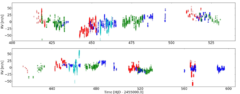
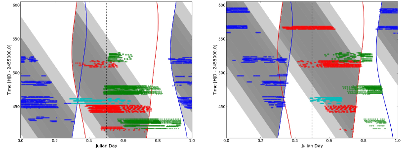
Figure 2: Radial velocity curve of $\gamma$ Psc (top panel) and $\theta^{1}$ Tau (bottom panel). The radial velocities of $\theta^{1}$ Tau have been detrended for the binary orbit, shown in Fig. 4. The red, blue, green, and cyan data points have been acquired with the Hermes, Hides, Coralie, and Sophie spectrograph, respectively.

Figure 3: Distribution of the radial velocity measurements of $\gamma$ Psc (left panel) and $\theta^{1}$ Tau (right panel). The same color code as in Fig. 1. For Hides and Hermes, also the value of the airmass X at which the target was observed is shown. Light gray shaded areas indicate 2.5 $<$ X$<$ 3 and dark gray X $<$2.5. The solid blue and red lines indicate the nautical dawn for Hides and Hermes, respectively.

To use the observing time efficiently, we were searching for a target combination, that encompasses two targets, separated by approximately 5 hours in right ascension. After testing several target combinations, we finally selected the G9III star $\gamma$ Psc (HD 219615) and the K0III star $\theta^{1}$ Tau (HD 28307) as targets for our campaign.

2.2 Characteristics of $\gamma$ Psc and $\theta^{1}$ Tau

Both targets are evolved stars which are expected to exhibit solar-like oscillations. An overview of the fundamental parameters of these stars from the literature is given in Table 2. $\gamma$ Psc is a single field star which was studied frequently in the past using photometric and spectroscopic measurements (e.g. Luck & Heiter, 2007; Hekker & Meléndez, 2007). The most important feature of $\gamma$ Psc with respect to the present study is its subsolar iron abundance (Table. 2).

$\theta^{1}$ Tau is one of the four giants in the Hyades cluster and a well studied binary (e.g. Lunt, 1919; Torres et al., 1997; Lebreton et al., 2001; Griffin, 2012). The Hyades have a slightly higher metallicity than the Sun with Fe/H = +0.1 (Takeda et al., 2008). By comparing theoretical isochrones matching the measured Helium and metal content of the cluster, Perryman et al. (1998) found a main-sequence turn off point of $\sim$2.3 M_⊙ which corresponds to a cluster age of 625$\pm$50 Myr. Therefore only the most massive stars are already in more advanced evolutionary stages after the main sequence. Very recently, Auriere et al. (2014) reported on the detection of a magnetic field in $\theta^{1}$ Tau whose unsigned longitudinal component peaked to 3$\pm$0.5 G. From their measurements they find indications for a complex surface magnetic field structure.

Interferometric observations allow for a radius determination, independent of seismology. Interferometric observations of the Hyades’ giants were published by Boyajian et al. (2009), reporting a radius of 11.7$\pm$0.2 R_⊙ for $\theta^{1}$ Tau. For $\gamma$ Psc no such observations are reported in the literature. We therefore obtained interferometric observations of this star with the Amber instrument at the Very Large Telescope Interferometer (VLTI, cf. Section 3).

2.3 Participating observatories

The main part of the campaign took place from August 2010 through January 2011 and utilised 5 different telescopes.We monitored $\gamma$ Psc and $\theta^{1}$ Tau for $\sim$120 d and $\sim$190 d, respectively, during which in total 8844 spectra were taken with the Hermes, Coralie, Sophie, Hides and Sarg spectrographs.

The majority of data was obtained with the Hermes spectrograph (Raskin et al., 2011) mounted at the 1.2 m Mercator telescope on La Palma, Canary Islands, the Coralie spectrograph (e.g. Queloz et al., 2000) operated from Mercator’s twin 1.2 m Euler telescope on La Silla, Chile and the Hides spectrograph (Izumiura, 1999) at the Okayama 1.88 m telescope, Japan. We used the commissioning time of the fibre-fed high-efficiency observing mode of Hides for the campaign (Kambe et al., 2013). Additional data was acquired with the Sophie spectrograph (Bouchy et al., 2009) at the 1.93 m telescope at the Observatoire de Haute-Provence (OHP) in the south of France. During the phase of best visibility for both targets, we obtained spectroscopic data with the Sarg spectrograph (Gratton et al., 2001) mounted at the 3.58 m Telescopio Nazionale Galileo (TNG), on La Palma. Due to problems in the reduction of the Sarg data, they could not be included in the present analysis. An overview of the applied calibration techniques, the observers and the number of spectra taken with each instrument is given in Table 2.

Additionally, for $\gamma$ Psc we applied for and obtained two half nights with the Amber instrument at the Very Large Telescope Interferometer (VLTI), using the 1.8m auxiliary telescopes (See Section 3).

In 2007 the MOST satellite (Walker et al., 2003) was used to search for photometric variability in the Hyades’ giants. The MOST team kindly provided us with the previously unpublished light curve of $\theta^{1}$ Tau, covering 22 days to compare the photometric and the radial velocity variations (See Section 6.2).

2.4 Radial velocity measurements and data set merging

In order to achieve ms^-1 precision in our radial velocity measurements, we utilised the available simultaneous calibration techniques. The Hermes, Coralie and Sophie spectrographs use Thorium-Argon (ThAr) or Thorium-Argon-Neon (ThArNe) reference lamps, from which light is simultaneously fed to the spectrograph through a reference fibre. On the CCD, the stellar and the reference spectrum are alternating in position. Radial Velocity information was derived from the spectra using the instrument pipelines. Hides use the absorption spectrum of an Iodine (I₂) cell, superimposed on the stellar spectrum in a wavelength range of 500 to 620 nm. Hides data was reduced with IRAF and the radial velocity was estimated with the method described in Kambe et al. (2008) by a member of the Hides team.

The mean radial velocity of each data set was subtracted from the observations of $\gamma$ Psc to merge the results from all 4 different telescopes, in order to obtain a consistent radial velocity curve. As $\theta^{1}$ Tau is a binary, we subtracted an orbital model (Table 4, Figure 4), derived from the data set of Griffin (2012), equally distributed over 40 years (from 1969 through 2010). As we have no overlap of data, except for about 1 hour between Hermes and Coralie and only a few radial velocity standards were observed, we manually corrected the offsets between the radial velocities from different spectrographs.

In addition to the data of Griffin, we also monitored the radial velocity of $\theta^{1}$ Tau with Hermes between early 2010 up to late 2013. The radial velocity values from Griffin (2012) as well as from our monitoring, listed in Table 4 are compared in the phase diagram, depicted in Figure 4.

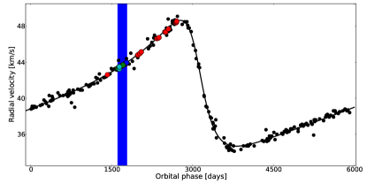
Figure 4: Orbital velocity phase diagram of $\theta^{1}$ Tau. Data by Griffin (2012) between the years 1969 and 2010 is shown as black dots. The duration of our multisite asteroseismology campaign is marked with the blue bar. Red dots mark the values from the ongoing radial velocity monitoring with the Hermes spectrograph. The values are reported in Table 4.

Table 3: Orbital parameters for $\theta^{1}$ Tau.

P	T0	$e$	$\omega$	K	$\gamma$
$[$d$]$	[d]		[rad]	[km s-1]	[km s-1]
5927$\pm$7	2439132$\pm$12	0.56$\pm$0.01	1.20$\pm$0.01	6.99$\pm$0.05	40.23$\pm$0.03

Table 4: Radial velocities of $\theta^{1}$ Tau from Hermes observations in the high-resolution observing mode.

HJD	RV	errorRV
$[$d$]$	[km s-1]	[km s-1]
2455241.38046	41.645	0.001
2455799.74878	43.793	0.002
2455806.74723	43.826	0.001
2455809.75936	43.865	0.001
2455842.75045	44.008	0.001
2455870.65140	44.186	0.001
2456157.69844	45.671	0.001
2456179.69122	45.704	0.001
2456305.41881	46.401	0.001
2456317.38334	46.396	0.001
2456322.38404	46.398	0.001
2456374.35806	46.738	0.002
2456507.72800	47.417	0.002
2456510.72944	47.419	0.001
2456518.71171	47.494	0.002
2456523.74224	47.481	0.002
2456526.74136	47.590	0.002
2456576.53391	47.681	0.001

An inspection of the combined data subsets, as depicted in Figure 1, shows that both stars exhibit radial velocity variations. The colours of the data points show the contribution of the different observatories. Although from single-site data the long periodic variations of $\gamma$ Psc could be seen as long periodic trends, it becomes evident from the combination of multi-site data that it is a clear oscillation signal. Figure 1 also suggests that $\theta^{1}$ Tau oscillates at higher frequencies than $\gamma$ Psc. The full radial velocity curves are shown in Fig. 3.

Figure 3 visualises the observational coverage of our campaign in an échelle diagram style. The vertical axis of both diagrams shows the distribution of observations during the project from August 2010 to January 2011. The horizontal axis shows the time of the day as fraction of the Julian day. It therefore depicts the coverage of the multisite campaign. For a more intuitive understanding of the diagram, the airmass of the object and the laps of the nautical twilight are given for the geographical location of the Hides and Hermes spectrographs.

For improving the agreement between different data sets while merging, and for increasing the signal-to-noise ratio in the amplitude spectrum, we normalised the uncertainties of the individual radial velocity measurements following the approach developed by Butler et al. (2004) and Bedding et al. (2007), which was described and adopted by Corsaro et al. (2012b). The analysis consists of two steps. First, the individual uncertainties in the radial velocity measurements are rescaled in order to be consistent with the amplitude of the noise level in the amplitude spectra, $\sigma_{\mathrm{amp}}$, which is measured for each data set separately in a region far from the power excess. Second, a residual time-series is derived by a complete pre-whitening of the oscillation signal, in order to end up with only noise remaining in the data sets.

The results of this approach in the case of Hermes data for $\gamma$ Psc is depicted in Fig.5. The upper panel shows the observed cumulative histogram of the ratio $|r_{i}/\sigma_{i}|$ of the residuals $r_{i}$ to the original uncertainty $\sigma_{i}$ in each radial velocity measurement (black diamonds) with the theoretical distribution expected for Gaussian noise (red line). The uncertainty of the individual radial velocity measurement is then adjusted by the ratio $f$ of the two distributions, which is shown in the lower panel. The ratio enhances the presence of a number of outliers, i.e. data points deviating from the expected distribution with $|r_{i}/\sigma_{i}|>1.2$, which are down-weighted when computing the amplitude spectrum.

Table 5: Accuracy per measurement of the radial velocity observations.

		original uncertainties		normalised uncert.
$\gamma$ Psc	N	$\sigma_{\rm noise}$	$\sigma_{\rm meas.}$	$\sigma_{\rm noise}$	$\sigma_{\rm meas.}$
		[m s-1]	[m s-1]	[m s-1]	[m s-1]
Hermes	1316	0.3	7.3	0.3	7.4
Coralie	1946	0.2	7.2	0.2	6.6
Hides	1306	0.1	4.2	0.1	3.6
Sophie	485	0.6	10.8	0.5	8.7
All	5053	0.1	7.0	0.1	5.4
$\theta^{1}$ Tau	N	$\sigma_{\rm noise}$	$\sigma_{\rm meas.}$	$\sigma_{\rm noise}$	$\sigma_{\rm meas.}$
		[m s-1]	[m s-1]	[m s-1]	[m s-1]
Hermes	1286	0.1	3.5	0.1	4.1
Coralie	790	0.2	4.4	0.2	4.5
Hides	1283	0.1	2.3	0.1	2.1
Sophie	360	0.6	9.7	0.4	6.1
All	3719	0.1	4.3	0.1	3.0

As a conclusion, we were able to reduce the noise level in the amplitude spectrum of the master data set from $\sigma_{\rm amp}=0.09\,$m s^-1 to 0.06 m s^-1 for $\theta^{1}$ Tau, and from $0.12$ m s^-1 to $0.1$ m s^-1 for $\gamma$ Psc. These values are the mean noise amplitude, derived for the frequency range 1000$-$1200 $\mu$Hz of the power spectrum which is supposedly free from leakage of oscillation power. The values of the mean noise amplitude in this range and how they were modified through the normalisation of weights is shown in Table 5. The frequency analyses of these data are presented in Sections 5 and 6 and were performed on these adjusted residual radial velocity curves.

2.5 Instrument commissioning of Hermes

The campaign was also used for commissioning the fibre-fed high efficiency observing mode of the simultaneous ThArNe observing (low resolution with reference fibre, i.e. LRFWRF) of the Hermes spectrographs. In this observing mode, Hermes is simultaneously fed from the telescope and a ThArNe calibration unit through 60 $\mu$m fibres. The exposure times were chosen to achieve a signal-to-noise ratio of 150 in the blue part of the stellar spectrum. To avoid saturation of the emission line spectrum and an eventual contamination of the stellar spectrum through blooming of strong lines on the CCD chip, a neutral density filter regulates the intensity of the reference source. The obtained spectra were reduced with the instrument specific pipeline, extracting a 1D spectrum for the stellar and reference fibre. From each spectrum, the radial velocities of the star were derived through cross-correlation of the wavelength range between 478 and 653 nm with a line-list template of the spectrum of Arcturus (Raskin et al., 2011). The radial velocities are then corrected for the shift in radial velocity, determined from the cross correlation of the simultaneously exposed ThArNe spectrum with the reference ThArNe spectrum, obtained in the beginning of the night.

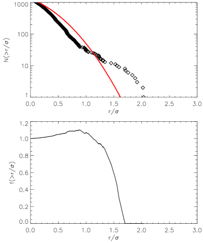
Figure 5: Cumulative histograms for Hermes observations of $\gamma$ Psc. Upper panel: The diamonds represent the ratio $|r_{i}/\sigma_{i}|$ between the residuals in the pre-whitened time-series and the uncertainties of each radial velocity measurement. The solid red curve depicts the result expected for Gaussian noise. The diagram in the lower panel shows the ratio between the observed and theoretical distribution of the uncertainties.

2.5.1 $\delta$ Eri

To test the performance and the accuracy of the observing mode before the campaign, we have obtained observations of $\delta$ Eri, a well known solar-like oscillator, exhibiting power between 500-900 $\mu$Hz (Carrier et al., 2003). Our data set covers 14.4 hours in two consecutive nights in late November 2009. In total, 235 spectra have been obtained with an exposure time of 60 to 90 seconds. The resulting radial velocity time series and the corresponding power spectrum of $\delta$ Eri are shown in Figs. 7 and 7.

From the comparison with earlier observations obtained by Carrier et al. (2003), we find that the region between 1500 and 4000 $\mu$Hz is free from contamination through oscillations and resembles the average amplitude $\sigma_{\rm noise}$, which originates from instrumental noise and other noise sources. Following the Parseval theorem, we obtain

$$\sigma_{\rm measurement}=\sqrt{\frac{2\cdot N}{\pi}}\cdot\sigma_{\rm noise},$$ (1)

the average noise amplitude of 0.24 m s^-1 in this region translates into an accuracy of about 2.9 m s^-1 per measurement which is more than sufficient to explore solar-like oscillations in red-giant stars. These observations were obtained in an early phase of the commissioning. As the instrument was improved since the observations of $\delta$ Eri, we did not find such noise in the data set of the campaign in 2010. Therefore, the noise in this frequency region is likely be coloured noise, originating from instrumental effects. These observations of $\delta$ Eri thus provided us with a proof-of-concept for the main observing campaign.

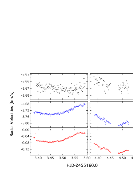
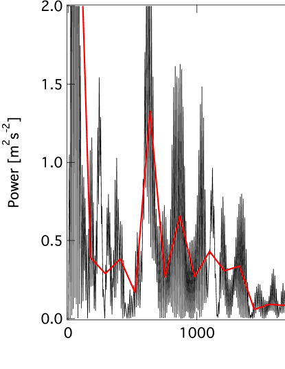
Figure 6: Radial velocity of $\delta$ Eri. Top panel shows the radial velocity values corrected for radial velocity drifts. The middle panel shows the uncorrected velocity values from the stellar spectrum while the bottom panel gives the radial velocity drift of the simultaneous ThArNe with respect to the wavelength reference, obtained in the beginning of the night.

Figure 7: Power spectrum for the RV measurements of $\delta$ Eri. The red line illustrates the running average noise level in the spectrum.

2.5.2 $\gamma$ Psc and $\theta^{1}$ Tau

We performed the same analysis for $\gamma$ Psc and $\theta^{1}$ Tau for the frequency range between 1000 and 1200 $\mu$Hz on the campaign data, because we did not detect the signature of spectral leakage of oscillation power in this region. We calculated the noise amplitude for this region and estimated the accuracy per measurement from Eq. (1) for individual data sets. An overview is given in Table 5.

The numbers in Table 5 show that, although both stars were observed with the same instruments, the intrinsic scatter in the power spectra of $\gamma$ Psc is consistently 1.8 times higher than for $\theta^{1}$ Tau. One possible explanation for this velocity jitter could be systematic effects as the accuracy of the measurements depend on how suited a star template for the cross correlation is for a given star. All pipelines used templates for K0 stars. Carney et al. (2003) concluded that neither orbital motion nor pulsation can explain such velocity jitter and suggest star spots or activity as another possible explanation.

3 Interferometric observations of $\gamma$ Psc

The AMBER instrument (Petrov et al., 2007) on the Very Large Telescope Interferometer (VLTI) was used to observe $\gamma$ Psc in its low spectral resolution (LR) observing mode (R=30), covering the J, H and K atmospheric bands. Observations were procured during the nights of 4 and 5 October 2010, using two triplets of Auxiliary Telescopes (ATs) that included stations A0 and K1, the longest baseline (128m) available at that time (see Table 6). The VLTI first-generation fringe tracker FINITO (Le Bouquin et al., 2008) was used to track the fringes.

3.1 Reduction

The data reduction was performed with the standard software amdlib v3.0.5, provided by the Jean-Marie Mariotti Center (JMMC) (Tatulli et al., 2007; Chelli et al., 2009). With amdlib, first a P2VM (Pixel-To-Visibility-Matrix) is computed, which is then used to translate the detector frames into interferometric observables. In our case, a typical exposure consisted of 1000 frames, with integration times of 25 ms each. For each exposure, a frame selection and averaging is subsequently performed, typically using a S/N-based criterion. In the final raw data product additive biases should be removed, leaving only multiplicative terms to be divided away in the calibration stage. To this end, each sequence of five science (SCI) exposures is interleaved with similar sequences on well chosen calibrators for which the visibility can be predicted with high precision. The estimated transfer function contains residual effects from the atmosphere, as well as the interferometer’s response to a point source.

Table 6: Observing log of the AMBER LR data.

Date	MJD	Calibrator	Stations	DIT	NDIT	FINITO
				[s]
2010 Oct 05 (a)	55474.11	-	A0-K0-I1	0.025	1000	ON
2010 Oct 06	55475.11	HD215648(b)	A0-K0-G1	0.5	120	ON
2010 Oct 06	55475.16	HD215648	A0-K0-G1	0.1	1000	ON

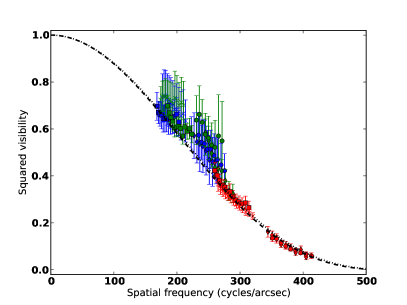
Figure 8: Left panel: the calibrated squared visibilities of $\gamma$ Psc. The colour denotes the baseline: K0-G1, A0-G1 and A0-K0 are shown in blue, green and red, respectively. The dashed and dotted lines are the best-fit UD angular diameters in the H and K bands. Different symbols are used to represent the two calibrated exposures in the H (circles and diamonds) and K (squares and crosses) band. Right panel: the closure phases as a function of the longest spatial frequency in the triplet. The same symbols are used as in the left panel, but the colour now denotes the exposure (blue being the first).

During the first night only one sequence of exposures of the science target could be obtained, as well as a sequence on a check star that has the same expected angular diameter. Since no proper calibrator (CAL) could be observed, these data were not retained in our analysis. Two sequences of CAL-SCI-CAL were obtained in good observing conditions (seeing $\sim$0.7$\arcsec$) during the second night. With a minimal S/N of $\sim$2 at the longest baseline in the J band, where the VLTI throughput is low and the visibility is close to null, the intrinsic data quality is very good. This is also evidenced by the small spread between the subsequent exposures in each sequence. Despite the good S/N, the J band data were discarded for two reasons. First, the wavelength-calibration is particularly unreliable in the J band. There is no way to do it reliably in the LR observing mode, so what amdlib does is to fit the position of the discontinuity between the H and K bands to its expected wavelength value. This works reasonably in the H and K bands, with an estimated systematic uncertainty of 2%, but leads to much larger uncertainties in the J band. Since the wavelength is used in the computation of the P2VM, and determines the spatial frequency of the observation, a wrong wavelength table can significantly bias the final result. Second, the spatial average of the phase of the incoming wave front (i.e. piston, cf. Vérinaud & Cassaing, 2001) and its spread is large in the J band.

The critical step in the AMBER data reduction is the selection and averaging of frames within one exposure. Depending on the performance of FINITO, the contrast of a frame can be reduced by the residual effect of atmospheric jitter. At the time of our observations no realtime FINITO data were recorded yet, so there is no objective way to do the frame selection. Instead, we resorted to the classical approach and selected frames based on piston ($<\,10\,\mu$m) and S/N (best 15%) for the squared visibilities, while the 80% frames with the best S/N were retained for the closure phases as these are not sensitive to piston. The used criteria are a trade-off between competing effects: a too large piston will bias the visibilities, while a too strong selection criterion on piston will reduce the S/N too much and might bias the visibilities as well. In general, very little frames were removed based on piston, indicating that FINITO locked on the fringes properly, except in the H band on the longest baseline. For the latter we note a systematic piston offset from zero which appears in both science measurements, despite their different detector integration times (DIT). Although the calibrator measurements are affected similarly, the brightness difference between the science target and the calibrator might result in a residual effect after the calibration. Different selection criteria were tried, and we estimate a maximum bias on our derived angular diameter, due to our choice of selection criteria, of $\sim$3% in K and $\sim$6% in H.

Figure 9: The $\chi^{2}_{\rm r}$-map of the limb darkened angular diameter versus the linear limb darkening coefficient.

The error on the final calibrated visibilities and closure phases is the quadratic sum of the intrinsic error on the science measurement, estimated from the spread between the consecutive exposures, with an error term for the transfer function. The latter is computed as the quadratic sum of the intrinsic error on the calibrator measurement with the uncertainty on the calibrator’s theoretical visibility, and the spread between the different calibrator measurements. The transfer function was very stable on the longest baseline, but less so on the shorter ones; hence the large difference in the errors.

Special care was taken to estimate the wavelength-dependent uniform disk (UD) angular diameter of the calibrator. First, a bolometric diameter is determined from SED-fitting (using the grid-based procedures of Degroote et al., 2011). Then the formula from Hanbury Brown et al. (1974)

$$\frac{\theta_{LD}}{\theta_{UD}}=\sqrt{\frac{1-\alpha_{\lambda}/3}{1-7\alpha_{\lambda}/15}}$$ (2)

was used to convert from bolometric to UD diameter. $\alpha_{\lambda}$ is the band-dependent linear limb darkening coefficient for the appropriate stellar parameters, and is taken from the catalogue of Claret & Bloemen (2011). Since we use the ATLAS (Kurucz, 1993) plane-parallel atmosphere models, the fitted bolometric diameter can be assumed equal to the limb-darkened diameter used in Eq. (2) (see e.g. Wittkowski et al., 2004, for a more detailed discussion about this assumption). The derived value (listed in Table 6) agrees perfectly with the diameter provided by the JMMC’s SearchCal tool (Bonneau et al., 2006).

The final calibrated squared visibilities and closure phases are graphically depicted in Fig. 8. The visibility precision on the longest baseline is high, in contrast to the other baselines. The closure phases are very precise in the K band ($\sim$1-2^∘), and a bit less precise in H ($\sim$3-5^∘), but all are zero within 3$\sigma$.

3.2 Analysis

Fitting of simple geometric models to the interferometric data was performed with the LITpro software tool (Tallon-Bosc et al., 2008) that is provided by the JMMC. LITpro does a simple but fast $\chi^{2}_{\rm r}$-minimisation, that also allows for easy examination of correlations between parameters through the computation of a correlation matrix and $\chi^{2}$-maps. Given the measured closure phases of zero degrees, we only fitted point-symmetric models to the squared visibilities. First we try a uniform disk brightness profile. The H and K band were treated separately to account for the difference in the object’s limb darkening and the AMBER systematic errors. The best-fit uniform disk curves are shown in Fig. 8 and have diameters of $\theta_{UD}^{H}$=2.29$\pm$0.03 and $\theta_{UD}^{K}$=2.26$\pm$0.04 mas. Since LITpro assumes each data point to be independent, while the different AMBER wavelength channels are correlated, we here corrected LITpro’s statistical errors using $\sigma=\sqrt{N_{ch}}\sigma_{stat}$. The corresponding $\chi^{2}_{\rm r}$ values (with its $\sigma$) are 1.3$\pm$0.2 and 0.8$\pm$0.2 for the H and K bands respectively. Although the data do not require a more complex model, it is useful to fit a limb darkened model to check for internal consistency and because it is the limb darkened diameter that should be used for comparison with the seismic value. For simplicity we use a linear limb darkening law.

We note that the visibilities at shorter baselines are systematically above the model fit (Figure 8). This is known to be the result of a calibration with poor transfer function stability (which is mostly systematic across all wavelengths, i.e. it is to be expected that all visibilities fall on the same side of the model curve). Moreover, the diameter is constrained mostly by the measurements at the highest spatial frequencies which have a higher resolving power and in this particular case also a more stable transfer function.

Figure 9 shows the $\chi^{2}_{\rm r}$-map of the limb darkened K band angular diameter versus the linear limb darkening coefficient. Since our spatial frequencies only cover the first lobe of the visibility curve, the limb darkening cannot be constrained independently. However, for a given limb darkening coefficient we can determine the corresponding diameter. Taking the linear limb darkening coefficients from Claret & Bloemen (2011), using the parameters of $\gamma$ Psc, which are $\alpha_{K}\in{[0.28,0.31]}$ and $\alpha_{H}\in{[0.33,0.36]}$, together with Eq. (2) and the measured UD diameters, we find limb darkened diameters of $\theta_{LD}^{H}$=2.4$\pm$0.1 mas and $\theta_{LD}^{K}$=2.31$\pm$0.09 mas, respectively. The (conservative) errors are quadratic additions of all mentioned error terms. These limb darkened diameters agree well with the directly fitted values for the same value of $\alpha_{K}$ and $\alpha_{H}$ (see e.g. Fig. 9). A global fit to the full data set, and assuming the limb darkening coefficients $\alpha_{K}=0.295$ and $\alpha_{H}=0.345$, results in a final angular diameter of $\theta_{LD}=2.34\pm 0.10$ mas. With a Hipparcos parallax distance of $42.3\pm 0.3$ pc, this angular diameter translates into a linear radius of $10.6\pm 0.5$ R_⊙.

4 Long periodic variations

For both stars, the spectroscopic time series depicted in Fig. 3 reveal radial velocity variations on time scales longer than 100 d, which are present in the data sets of all sites separately. Such variations are too low in frequency to be connected to solar-like oscillations.

For the determination of these long periods, only data sets spanning over more than 100 days were used, i.e. Hermes, Coralie, and Hides. The data set from Sophie was excluded from this analysis, as it only covers about a week in time and suffers from strong night to night zero-point shifts. Also the last observing run on $\theta^{1}$ Tau with Hermes in early January 2011 was excluded from the period determination due to zero-point shifts. We determined the periods by fitting a sine-wave to the variation in the data subset, using Period04 (Lenz & Breger, 2005).

Table 7: Long periodic variations found in the campaign stars.

Star	Period	Amplitude	Phase	S/N
	[d]	[m s-1]
$\gamma$ Psc	113.0$\pm$0.8	22.8$\pm$0.3	0.789$\pm$0.002	6.4
$\theta^{1}$ Tau	165$\pm$3	9.3$\pm$0.2	0.439$\pm$0.004	6.4
	16.57$\pm$0.05	4.7$\pm$0.2	0.061$\pm$0.007	4.1

Figure 10: MOST photometry of $\theta^{1}$ Tau, deconvolved from thermal trends.

Figure 11: Comparison of the power spectra of $\gamma$ Psc from the single instruments. The top panels show the original and the smoothed signal in the PDS for individual data sets. Two PDS are shown in the case of Hermes: the full data set was used for the red PDS and the set corrected for the radial velocity jump at 445 days (Fig. 3) was used for the black PDS. The estimate of $\nu_{\mathrm{max}}$ as the highest point of the smoothed PDS is marked as dotted vertical line for each individual data set. The bottom panel shows the PDS of the combined data set, divided into two halves. The first and second half of the data set are shown as grey and black line. The red line shows the power spectrum of the RV-subset with the best coverage (440$<t<$465 days in Fig. 3).

For $\gamma$ Psc we find a variation with a period of 113 d and a semi-amplitude of 22.8$\pm$0.3 ms^-1. $\theta^{1}$ Tau shows a dominant variation with a period of 165 d with 9.3$\pm$0.2 ms^-1 and a smaller variation on the order of 16.57 days (Table 7), which appears to be one-tenth of the main period. The close up on the radial velocity data of $\theta^{1}$ Tau in the bottom panel of Fig. 1 shows that all three data sets are modulated by this intermediate frequency.

Although we only cover a bit more than 1 cycle, we argue that these variations are real, as they occur in data sets from independent telescopes. Instrumental trends for a given star would not be consistently present with the same time scale and amplitude in both stars in independent data sets. In Fig. 3, all single-site data sets have been shifted by a constant offset in radial velocity. The variations in radial velocity follow a particular pattern throughout the full time span, independent of the used instrument. We therefore conclude that these trends are intrinsic to the stars.

Estimating the rotation period from the values of the stellar radius and the projected surface rotation velocity in Table 2, points toward a period of 113 and 138 days for $\gamma$ Psc and $\theta^{1}$ Tau, respectively. This is a perfect match to the period of 113$\pm$0.8 d we found in $\gamma$ Psc and suggest that the inclination of the rotation axis of $\gamma$ Psc is close to 90^∘. For $\theta^{1}$ Tau the expected value deviates by $\sim$30 days from the 165$\pm$3 d variation, found from our analysis. Torres et al. (1997) and Griffin (2012) have reported that the inclination of the eccentric binary orbit is probably close to 90 degrees. However, it is questionable if the orbital inclination is identical to the inclination of the rotation axis. For the eccentric system KIC 5006817, Beck et al. (2014) did not find a good match for between the two axes. The orbital and rotation axis could be inclined by a few degrees. Yet, a lower inclination does not explain this difference.

In the literature, we find independent proof of the long periodic variability of $\theta^{1}$ Tau. The peak-to-peak amplitude we measure for $\theta^{1}$ Tau is compatible with the radial velocity scatter of $\sim$20 ms^-1, found by Sato et al. (2007) in the residuals of the binary model. The emission in the Ca ii H and K lines at 393.4 and 396.9 nm, respectively shows that $\theta^{1}$ Tau as well as $\gamma$ Psc are chromospherically active. From about a decade of observations, Choi et al. (1995) found that the Ca ii H and K emission in $\theta^{1}$ Tau varies with a mean period of 140$\pm$18 days, which is in agreement with our value of 165$\pm$3 days. Given that our value is determined from only a bit more than one stellar revolution, we conclude that we measured the surface rotation of $\theta^{1}$ Tau but that our value could be affected by activity or the short temporal base line. The found long periods are typical rotation periods for red giants. Indeed, following a different approach, Beck et al. (2014) derived a similar period of 165 days for the surface rotation from forward modelling of the rotational splitting of dipole modes in the red giant component of KIC 5006817. Although this star a radius of only 6 R_⊙, this seismic result points to the same period regime of surface rotation. Ongoing studies of surface rotation of red giants from solar-like oscillations from Kepler photometry point to the same regime of rotation frequencies and show that there is a large spread of rotation periods that depends on the individual rotation history of the star (e.g. Garcia et al., 2014; McQuillan et al., 2014).

We note that rotation does not explain the 5 m s^-1 variation on 16.5 days found for $\theta^{1}$ Tau. The available MOST photometry suggests variations on the order of 11 days (Fig. 10) such that variability with this type of periodicity is confirmed in this independent data set.

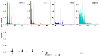
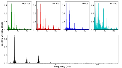
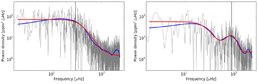
Figure 12: Spectral windows of $\gamma$ Psc (left panels) and $\theta^{1}$ Tau (right panels). The upper panels depict the spectral windows of the single-site data. The spectral window of the combined data set is shown in the lower left panel.

Figure 13: Power density spectrum of $\gamma$ Psc (left) and $\theta^{1}$ Tau (right). The original spectrum of the spectroscopic time series is shown in grey. The blue line shows the smoothed PDS. The red line depicts the multi component fit to the original PDS. For $\gamma$ Psc no Gaussian profile was fitted for $\nu_{\mathrm{max}}$. The vertical black line shows the adopted value of $\nu_{\mathrm{max}}$ for $\gamma$ Psc and $\theta^{1}$ Tau of $\sim$32 and 90$\mu$Hz, respectively. For both stars, Fig.1 shows the clear variations on these time scales in the time series.

5 Solar-like oscillations in $\gamma$ Psc

The radial velocity curve of $\gamma$ Psc, depicted in Fig. 1 and Fig. 3 (top panel) reveals the clear presence of long and multi periodic radial velocity variations. Such patterns cannot originate from noise or instrumental trends, as they are consistently present in independent single-site data sets. The key values to describe solar-like oscillations are the frequency of the maximum excess of oscillating power, $\nu_{\mathrm{max}}$, and the large frequency separation, $\Delta\nu$, between consecutive pressure modes of the same spherical degree $l$.

From a data set contaminated with zero-point shifts we cannot determine a precise value for the frequency of maximum oscillation power. A typical approach would consist of shifting all individual nights to their nightly mean and then determine $\nu_{\mathrm{max}}$ from the combined master spectrum. However, from visual inspection of the radial-velocity variations (cf. Fig. 1) we estimated the frequency of the oscillations for $\gamma$ Psc to be on the order of 2 to 3 per day. Therefore, shifting the nightly data sets by their zero point would act as a high-pass band filter which shifts power to higher values. From comparing the power spectra of zero-point shifted and unshifted data, we find that the frequency range up to $\sim$30 $\mu$Hz is severely affected, but also the distribution in the higher frequent part of the PDS is flattened. Such filter would change the shape of the power excess and mimic a higher $\nu_{\mathrm{max}}$. To avoid unnecessary manipulations of the background signal, we only prewhitened the intrinsic long periodic variation of 110 days.

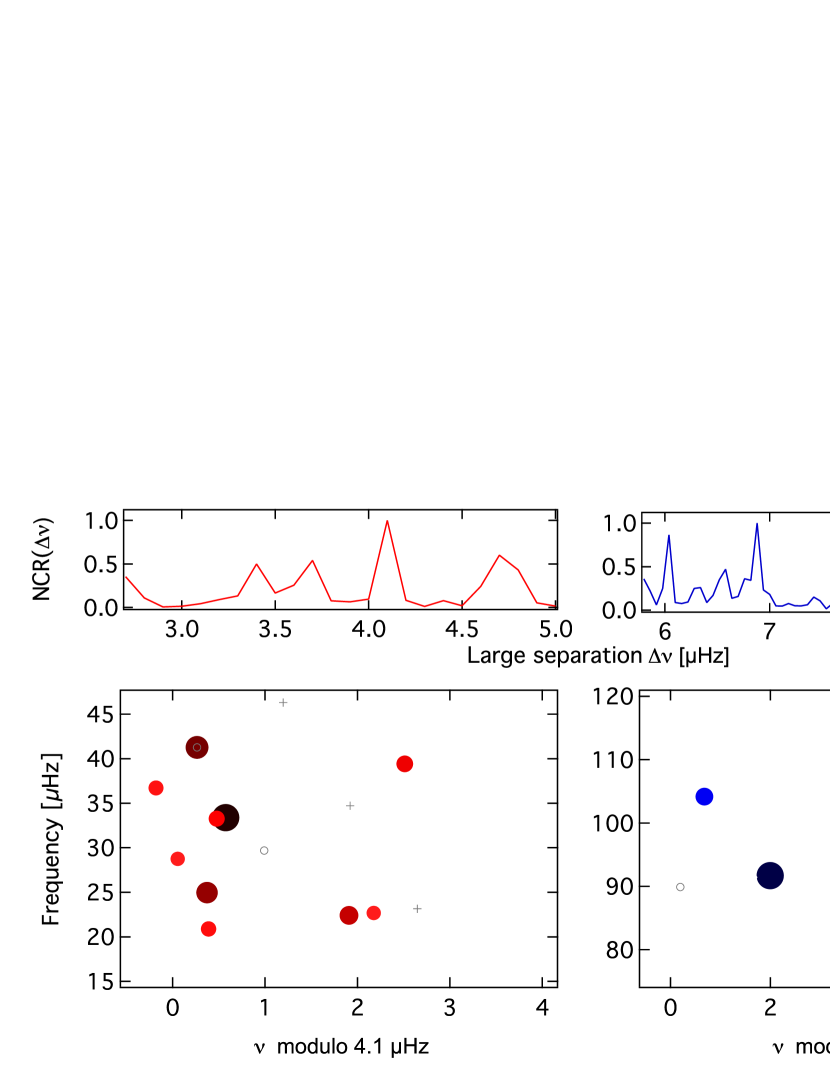
Figure 14: Frequency analysis of the combined data set for $\gamma$ Psc (left) and $\theta^{1}$ Tau (right). The top panels show normalised comb response (NCR) of the 6 strongest frequencies. The échelle diagrams (bottom panels) were calculated for the highest peak in the comb response function of $\gamma$ Psc and $\theta^{1}$ Tau, respectively. Solid dots represent modes with an S/N$\geq$5. Open circles show the original position of modes that were shifted by 11.574 $\mu$Hz. The crosses in the échelle diagram for $\gamma$ Psc mark the position of multiples of the daily aliases.

Before calculating the power spectrum for the full data set, the data sets for individual instruments were investigated. Nearly all single-site data already reveal a good approximation of the frequency of the oscillation power excess (Fig. 11, top panels). The Hermes data contain a source of instrumental noise that is dominated by long periodic noise and shows a maximum power at very low frequencies. This signal originates from small instabilities of the calibration lamp, which lead to night-to-night shifts. The main shift is visible in the red RV-curve in Fig. 3 between 440 and 460 days as a jump of $\sim$25 ms^-1. By correcting for this jump manually, the signal below $\sim$1 d^-1 drops (see Fig. 11, top left panel). For further understanding of the night-to-night shifts of the Hermes spectrograph, we have initialised a test program on Hermes during winter 2013/14.

From the smoothed power spectrum of the individual single data sets (Fig. 11, top panels), and the power spectrum of the combined data set (Fig. 11, red line in the lower panel) we identify the highest signal as the maximum oscillation power at $\sim$32 $\mu$Hz. Variations on this time scale are found from detailed inspection of all independent nightly data sets. Such long-periodic oscillations are expected for red giants higher up on the RGB or red clump stars and are compatible with the position of $\gamma$ Psc in the Hertzsprung-Russell diagram (HRD).

We subsequently combined all four single-site data sets of $\gamma$ Psc. The spectral window of the single-site data sets and the full data set for $\gamma$ Psc are presented in Fig. 13. The power excess of $\gamma$ Psc is located exactly at the knee of the power law, describing the long periodic granulation noise (Fig. 13). Although we see the peak of the power excess (or aliases of it, shifted by 11.6 $\mu$Hz) in the individual power spectra (Fig. 11), $\nu_{\mathrm{max}}$ is hardly visible in the power density spectrum of the combined data set. We argue that this is also a problem of the zero-point shift between data sets and nights. In addition, this region is contaminated by instrumental noise. It is therefore hard to reliably determine the value of $\nu_{\mathrm{max}}$ for $\gamma$ Psc from a multi-component fit (Fig. 13).

In a wide frequency range around the identified maximum of oscillation power (15-50 $\mu$Hz), all significant frequencies (i.e., S/N $\geq$ 5) were prewhitened, using the ISWF (iterative sine-wave fitting) method. The S/N compares the height of a mode to the mean noise in a selected frequency range. For $\gamma$ Psc it was determined between 50 and 70 $\mu$Hz. Indeed, we find the highest peaks around $\sim$32 $\mu$Hz.

The large frequency separation was then computed from the generalised comb-response (CR) function (Bonanno et al., 2008; Corsaro et al., 2012a), based on the six frequencies with the highest power. The extracted frequencies are available in the online material. With the CR function, we scanned a wide range of potential values of $\Delta\nu$, which includes a mass range that generously frames the mass estimates for the star in the literature. For $\gamma$ Psc the chosen range corresponds to $\sim$0.5 to $\sim$5 M_⊙ (Fig. 14). The values of $\Delta\nu$, suggested by the highest peaks were then tested with échelle diagrams.

The CR-function, calculated from the extracted peaks, exhibits a clear peak at $\Delta\nu$=4.1$\pm$0.1 $\mu$Hz (Fig 14, left upper panel). The uncertainty originates from a Gaussian fit to the main peak and given that we are dealing with ground-based and gapped data can only be taken as a lower limit. In addition, we tested different step-sizes of the CR function (up to 0.02 $\mu$Hz) but did not find a different result for the value and its uncertainty. This value remains stable up to the inclusion of the seventh highest out of the ten most significant frequencies. This is not surprising, because some of them are likely to be mixed modes, which do not follow the expected regular frequency pattern of pure p-modes. Using this value and the set of significant frequencies, we constructed an échelle diagram for this star, showing one ridge (Fig. 14). Most of the strongest modes are lining up on the left side of the diagram (i.e. $\nu$ modulo $\Delta\nu\leq 1$, hereafter termed échelle phase). We note that the échelle phase is closely related through the modulo operation to the parameter $\varepsilon$ from the asymptotic frequency relation (Aerts et al., 2010). One of the extracted frequencies is likely to be shifted by daily aliases. When we correct the strong mode at 29.7 $\mu$Hz for the daily alias, it also falls in the ridge of strong modes. The original and the shifted position of a mode in the échelle diagram are marked by open circles. This structure could be the ridge of radial and quadrupole modes. We can compare our identification to the $\varepsilon$-values found in large samples of red giant stars, observed with the Kepler space telescope (e.g. Huber et al., 2010; Corsaro et al., 2012b). For these stars we have a solid mode identification from uninterrupted data. Indeed, the study of Huber et al. (2010) shows that for a star with a $\Delta\nu$ of $\sim$4 $\mu$Hz, one expects a value of $\varepsilon$$\simeq$1 for radial modes suggesting that we correctly identified the radial modes. The remaining three extracted frequencies (at échelle phase of $\sim$2) may originate from mixed dipole modes, which is in agreement with $\varepsilon$$\simeq$1.5 for dipole modes. A comb-like pattern with a large separation of 4.1 $\mu$Hz cannot be explained by daily aliasing, as this value of $\Delta\nu$ is not a multiple of the daily alias (11.574 $\mu$Hz). For comparison the position of the daily alias frequencies are depicted as crosses in the échelle diagrams.

Following the scaling relations described by Kjeldsen & Bedding (1995), using the revised reference values of Chaplin et al. (2011), we estimate $\gamma$ Psc to be a star of M$\simeq$0.9 M_⊙ and R$\simeq$10 R_⊙. The stellar radius from the scaling relations is in good agreement with the independent radius of 10.6$\pm$0.5 R_⊙ from interferometric observations (see Section 3). The mass obtained from both scaling relations are below the mass derived from spectroscopic calibrations by Luck & Heiter (2007) to be 1.87 M_⊙. No uncertainty was given for this value. These values are likely affected by the lower constraining level of $\nu_{\mathrm{max}}$, if compared to the case of $\theta^{1}$ Tau (see Sect. 6). However, from the échelle diagram (Fig. 14) the value of the large separation appears convincing. By using the value of the large separation found from our oscillation spectrum of $\gamma$ Psc, and the independent radius from interferometry for the scaling relation for the stellar mass,

$$\frac{M}{M_{\odot}}=\left(\frac{\Delta\nu}{\Delta\nu_{\odot}}\right)^{2}\cdot\left(\frac{R}{R_{\odot}}\right)^{3}$$ (3)

we can derive the mass of the star without the use of $\nu_{\mathrm{max}}$. This approach leads to a mass of 1.1$\pm$0.2 M_⊙ for $\gamma$ Psc, which is in agreement with the mass found from the scaling relations. We therefore adopt 32 $\mu$Hz and 4.1 $\mu$Hz as good estimates of the $\nu_{\rm max}$ and $\Delta\nu$ in $\gamma$ Psc, respectively.

6 Solar-like oscillations in $\theta^{1}$ Tau

For $\theta^{1}$ Tau, we have two independent data sets, that we can analyse for the signature of oscillations. Besides our spectroscopic campaign, covering 190-days, we also have photometric data from the MOST satellite.

6.1 Spectroscopic campaign

The data sets of $\theta^{1}$ Tau reveal a clear signature of the power excess at 90$\pm$0.2 $\mu$Hz. The value of $\nu_{\mathrm{max}}$ was obtained from the fit of a power law plus a Gaussian profile and a constant noise background to the power density spectrum (Fig. 13). This value is a formal error from the fit and we note that this is unrealistically small.

To further improve the data, we corrected for zero-point shifts. As visible from Fig. 3 Sophie data suffer from severe night to night jumps. Also the last data from Hermes contain sudden jumps of up 50 ms^-1 (at $t>$560 d in Fig. 3). A visual inspection of the simultaneous ThArNe frames showed that these jumps originate from instabilities of the calibration lamp. Problematic frames were identified and deleted from the data set. The power excess of $\theta^{1}$ Tau is located at frequencies high enough that allow shifting the individual nights to their mean without manipulating the frequency region of $\nu_{\mathrm{max}}$. Therefore we subdivided the time string into individual nights and corrected them for the nightly mean. The frequency analysis was then performed at this time series of residuals. In total, we find 7 frequencies with an S/N$\geq$5 in the frequency range around $\nu_{\mathrm{max}}$. The extracted frequencies are available in the online material. From comparison with the MOST power spectrum, we find that the strong mode at 89.9 $\mu$Hz falls on top of the ridge structure when shifting by +1 d^-1. As we used the shifted data set for the prewhitening analysis, we could not use the background determined from the fit of the power-laws but derived the mean noise from the frequency range between 140 and 170 $\mu$Hz

The comb response function of $\theta^{1}$ Tau (Fig. 14, top right) is complex as it exhibits three peaks in the range of 6 $\mu$Hz $<\Delta\nu_{\rm CR}<$ 7 $\mu$Hz. The CR-function remains stable at this frequency range, independent of the number of significant oscillation peaks included and the resolution for which the CR-function is calculated. From the échelle diagram we can exclude $\Delta\nu_{\rm CR}$$\simeq$ 6$\mu$Hz, as by plotting all significant frequencies in an échelle diagram, inclined ridges form and it is close to half of the daily aliasing. This indicates a wrong trial value for $\Delta\nu$. Peaks above $\sim$8 $\mu$Hz can be excluded, as they suggest a mass below $\sim$1.5 M_⊙ and lead to a final radius ($\lesssim$8 R_⊙) which is $\sim$30 % smaller than the interferometric radius 11.7$\pm$0.2 R_⊙, determined by Boyajian et al. (2009). We therefore exclude these values from the possible solutions.

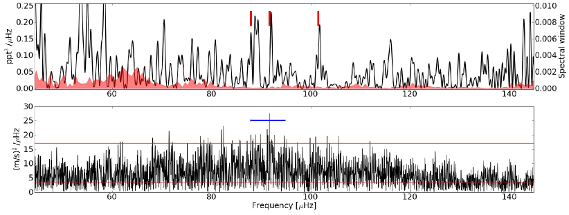
Figure 15: Comparison of the power spectra of the photometric and spectroscopic PDS of $\theta^{1}$ Tau. The top panel shows the power spectrum and the spectral window of the MOST data set as black line and red shaded region, respectively. The spectral window depicts the position of the orbital aliases and reveals that the range around $\nu_{\mathrm{max}}$ is nearly free of contaminations. The three main peaks in the region around 90 $\mu$Hz in the MOST spectrum, correspond to frequencies also detected with the ground-based campaign (red dashes). The bottom panel shows the unprewhitened power spectrum of the combined spectroscopic campaign data. The blue horizontal line indicates an average large frequency separation found for $\theta^{1}$ Tau. The lower and upper horizontal red line indicates the noise level and 5 times the noise level, respectively.

The highest peak in the CR-function indicates a large separation of 6.9$\pm$0.2$\mu$Hz. Again we note, that the error is likely to be an underestimate. The échelle diagram of $\theta^{1}$ Tau shows 8 frequencies with an S/N$\geq$5 folded with $\Delta\nu$ = 6.9 $\mu$Hz (Fig. 14, bottom right). From the scaling relations of Kjeldsen & Bedding (1995), we obtain from mass of 2.7$\pm$0.3 M_⊙ and a radius of 10.2$\pm$0.6 R_⊙ for a given $\Delta\nu$ =6.9$\pm$0.2 $\mu$Hz. For this value, the mass of the red giant primary of the $\theta^{1}$ Tau-system is well in agreement with the mass estimate provided by the orbital parameters and the Hipparcos dynamical parallax. Torres et al. (1997) reported a mass of 2.9$\pm$0.9 M_⊙ for the primary component, while using the parallax obtained from Hipparcos data Lebreton et al. (2001) derived a mass of 2.8$\pm$0.5 M_⊙ and 1.28$\pm$0.1 M_⊙ for the primary and secondary of $\theta^{1}$ Tau, respectively. All those values are substantially more massive than 2.3 M_⊙ of the turn off point in the Hyades as must be the case (Perryman et al., 1998).

While this value of 6.9 $\mu$Hz for the large frequency separation leads to a stellar radius that is slightly smaller than the interferometrically determined radius reported by Boyajian et al. (2009), there are indications that this interferometric radius is somewhat overestimated (by a few percent), to the extent that the disagreement is not significant. First, the diameters derived by Boyajian et al. (2009) for two other Hyades giants, $\delta^{1}$ Tau and $\epsilon$ Tau, are larger than other interferometric radii reported in the literature for these giants by 2-3 $\sigma$, and it is thus plausible that also their diameter for $\theta^{1}$ Tau is too large. Since Boyajian et al. (2009) were limited to a single baseline, calibrator, and observing night, the calibration may have suffered undetected systematics. Second, this reasoning is further corroborated by the disagreement between the spectroscopic effective temperature from Hekker & Meléndez (2007) and the T_eff derived by Boyajian et al. (2009), with the latter being 200 K lower than the former. This also suggests that the diameter derived by Boyajian et al. (2009) is slightly too large, as a T_eff derived from a bolometric flux and a radius (the method used by Boyajian et al. (2009)) scales inversely with assumed radius. For a more general discussion concerning possible biases in interferometric diameters, we refer to Casagrande et al. (2014). We therefore refrain from using this interferometric diameter as an argument against a seismic mass corresponding to 6.9 $\mu$Hz frequency spacing, and suggest the need for a new interferometric diameter determination, based on multiple baselines and calibrators. Given the required time frame of such an observational campaign, it is outside the scope of the current paper.

6.2 Oscillation in MOST space photometry

Independent confirmation of the intrinsic variability and oscillations in $\theta^{1}$ Tau is provided by the MOST space photometry. Figure 15 compares the power spectra of the MOST data set and the spectroscopic campaign. The variability of $\theta^{1}$ Tau is on the detection limit of the satellite. The spectral window of the data set, depicted as red shaded surface, shows that the power spectrum of the photometric measurements does not follow the shape of the spectral window and that the contamination by aliasing in this region is minor. A typical power density diagram can not be drawn, as the spectrum is dominated by the orbital aliasing. The main orbital alias frequencies are located well above this range at 164.35 $\mu$Hz (14.2 d^-1).

The strongest signal found in the photometric data is around 90 $\mu$Hz and located in a region without contamination. We find that the three highest peaks from MOST photometry coincide with significant frequencies from the spectroscopic campaign data set. These frequencies are marked with red dashes in Fig. 15. This independently confirms our detection of oscillation power in this region from the spectroscopic campaign data.

7 Conclusions

In this paper, we report on the spectroscopic multisite campaign performed in 2010, dedicated to the single field star $\gamma$ Psc and on $\theta^{1}$ Tau, the primary component of an eccentric binary system in the Hyades open cluster. This campaign was supported by interferometric observations from the VLTI and space data from the MOST satellite.

We found clear evidence of long and multi periodic variations in the radial velocity data set of $\gamma$ Psc. No precise value of $\nu_{\mathrm{max}}$ could be deduced due to contamination by granulation noise, and instrumental trends. However, we see clear indications, that $\nu_{\mathrm{max}}$ is located around $\sim$32 $\mu$Hz. This value is typical for red clump stars and agrees with the position of $\gamma$ Psc in the HRD. By analysing the frequency range around the adopted $\nu_{\mathrm{max}}$, we find a large separation of 4.1$\pm$0.1$\mu$Hz from the CR function. This value also leads to a convincing échelle diagram. The stellar radius from scaling relations shows good agreement with the radius from interferometry. We therefore estimate the mass of $\gamma$ Psc to be $\sim$1 M_⊙.

$\theta^{1}$ Tau exhibits a clear power excess at 90 $\mu$Hz in the spectroscopic data sets. Oscillations in this range and the dominant peaks are independently confirmed from MOST space photometry. According to the CR-function analysis a large separation of either 6.9 $\mu$Hz is preferred. Under the reasonable assumption that the interferometric radius of $\theta^{1}$ Tau (Boyajian et al., 2009) is overestimated, we find a rather good agreement between this value and the radius from the scaling relations. A new set of observations with the current instruments and the longest baselines on the CHARA array or similar instrumentation would allow a more reliable measurement of the radius of this star. The mass of $\theta^{1}$ Tau is 2.7$\pm$0.3 M_⊙.

$\theta^{1}$ Tau is of special interest due to its membership in the Hyades. Since 2010, the radial velocity of the binary system $\theta^{1}$ Tau has been monitored with Hermes. The binary is approaching its periastron passage early 2014. We hope to be able to perform a spectral disentangling analysis from these data.

In addition, we note that the value of the large separation for both stars comes from an attempt to measure the actual mean $\Delta\nu$ of the stars, because we only relied on the computation of the comb response function. Further investigations are needed to confirm these values. Unfortunately, the quality of the PDS does not allow to discriminate between the evolutionary stages from mixed mode period spacings. However, the frequency of the maximum oscillation power excess is typical for red clump stars.

Besides the solar-like oscillations, we also detected long periodic modulations of the radial velocities, which occur on the order of 113 days and 165 days for $\gamma$ Psc and $\theta^{1}$ Tau, respectively. These time scales are in good agreement with the estimates of the rotation period from the stellar radius and the measured $v\sin i$.

From this study we learned that the common approach to correct for zero-point variations by shifting the nightly data set of individual telescopes will suppress frequency information and shift $\nu_{\mathrm{max}}$ to higher frequencies for power excesses below $\sim$40 $\mu$Hz. We note, that also stars with $\Delta\nu$ $\simeq$11.6 $\mu$Hz, are very challenging from ground, as their large separation $\Delta\nu$ is identical to the 1-day aliasing in ground-based data. Very good spectral windows are needed to understand the oscillation spectra of such stars. Also, the interplay of solar-like oscillations and surface rotation requires a dense sampling and consistent data sets in order to disentangle the two effects. This can only be achieved with very dense telescope networks.

Finally, we note that in times of stunning asteroseismic results from space photometry, often the benefits of ground-based spectroscopy are forgotten. It is gradually becoming harder to successfully propose for sufficient telescope time for campaigns like the one described here. A promising future ground-based project is the Stellar Observations Network Group, SONG, which is a Danish led project to construct a global network of small 1 m telescopes around the globe (Grundahl et al., 2011). One of the main goal of the project is to obtain time series of radial velocity measurements with a high duty cycle, similar to our campaign. This will therefore allow us to investigate in detail the asteroseismic properties of the stars.