Atmospheric dynamics of terrestrial exoplanets over a wide range of orbital and atmospheric parameters

Abstract

The recent discoveries of terrestrial exoplanets and super Earths extending over a broad range of orbital and physical parameters suggests that these planets will span a wide range of climatic regimes. Characterization of the atmospheres of warm super Earths has already begun and will be extended to smaller and more distant planets over the coming decade. The habitability of these worlds may be strongly affected by their three-dimensional atmospheric circulation regimes, since the global climate feedbacks that control the inner and outer edges of the habitable zone—including transitions to Snowball-like states and runaway-greenhouse feedbacks—depend on the equator-to-pole temperature differences, patterns of relative humidity, and other aspects of the dynamics. Here, using an idealized moist atmospheric general circulation model (GCM) including a hydrological cycle, we study the dynamical principles governing the atmospheric dynamics on such planets. We show how the planetary rotation rate, planetary radius, surface gravity, stellar flux, optical thickness and atmospheric mass affect the atmospheric circulation and temperature distribution on such planets. Our simulations demonstrate that equator-to-pole temperature differences, meridional heat transport rates, structure and strength of the winds, and the hydrological cycle vary strongly with these parameters, implying that the sensitivity of the planet to global climate feedbacks will depend significantly on the atmospheric circulation. We elucidate the possible climatic regimes and diagnose the mechanisms controlling the formation of atmospheric jet stream, Hadley and Ferrel cells and latitudinal temperature differences. Finally, we discuss the implications for understanding how the atmospheric circulation influences the global climate.

1. Introduction

Since the mid-1990s, nearly 2000 planets have been discovered around other stars. The first to be discovered were giant planets with short orbital periods, and since then, many smaller planets with longer orbital periods have been identified. The planets can be generally divided into two types: planets close to their parent star that become synchronously locked, resulting in one side constantly being heated from their parent star, and asynchronously rotating planets with a diurnal cycle — similar to Earth and most solar system planets. In this study we focus on the latter type, and within these, we focus on terrestrial planets, i.e., those in which the atmospheric dynamics are limited to a thin spherical shell overlying a solid surface. These planets span a large range of masses, radii, densities, incident stellar fluxes, orbital periods, and orbital eccentricities. The goal of this study is to characterize the range of possible climatic regimes these planets might encompass, and characterize how the climate and habitability depend on these orbital, planetary, and atmospheric parameters.

Although exoplanet discovery and characterization began with giant planets, emphasis is gradually shifting to smaller worlds. Approximately 100 planets with masses less than $\sim 10$ Earth masses have been discovered, with many hundreds of additional candidates identified by the NASA Kepler spacecraft (Borucki et al., 2011). Planets toward the upper end of this mass range may typically constitute mini Neptunes with no solid surfaces (e.g., Valencia et al., 2007; Adams et al., 2008; Rogers et al., 2011; Nettelmann et al., 2011; Fortney et al., 2013), but planets toward the lower end are more likely terrestrial planets with solid surfaces and relatively thin atmospheres. Importantly, discoveries to date include a number of planets with masses and/or radii less than those of Earth (e.g., Fressin et al., 2012; Muirhead et al., 2012; Borucki et al., 2013; Barclay et al., 2013 see review by Sinukoff et al., 2013), as well as numerous planets $\sim 1-3$ Earth radii in size. This overall population of super Earths and terrestrial planets includes not only hot, inhabitable objects blasted by starlight (CoRoT-7b and Kepler-10b being prominent examples; Léger et al., 2011; Batalha et al., 2011), but also many planets receiving $\sim 0.2$ to several times the incident stellar flux Earth receives from the Sun, with effective temperatures of $\sim 200-400$ K (Muirhead et al., 2012; Dressing & Charbonneau, 2013; Quintana et al., 2014; see Figure 7 in Ballard et al., 2013 for a visual summary). Depending on atmospheric composition, these moderate stellar fluxes put these planets in or near the classical habitable zones around their stars.

Atmospheric characterization of super Earths, while difficult, has already begun. Attention to date has focused on GJ 1214b, a 6.5-Earth-mass, 2.7-Earth-radius super Earth orbiting a nearby M dwarf (Charbonneau et al., 2009). Transit spectroscopy in visible and near-infrared (IR) wavelengths indicates a relatively flat spectrum, ruling out hydrogen-dominated, cloud-free atmospheres and favoring instead a high-molecular-weight (e.g., water-dominated) atmosphere and/or the presence of clouds that obscure spectral features (e.g., Bean et al., 2010, 2011; Désert et al., 2011; Berta et al., 2012; de Mooij et al., 2012; Fraine et al., 2013; Teske et al., 2013; Kreidberg et al., 2014). The secondary eclipses of this relatively cool ($\sim 500$ K) planet have recently been detected by Spitzer (Gillon et al., 2014). The NASA Transiting Exoplanet Survey Satellite (TESS, to be launched in 2017) and ESA’s Planetary Transits and Oscillations of Stars satellite (PLATO, to be launched in 2024) will search for additional, observationally favorable super Earths, and upcoming platforms including the James Webb Space Telescope (JWST), the Characterizing Exoplanets Satellite (CHEOPS), and the groundbased Thirty Meter Telescope (TMT) and the European Extremely Large Telescope (E-ELT) will be capable of characterizing their atmospheres. These developments indicate that, in the coming decade, observational techniques currently used to characterize the atmospheres of hot Jupiters will be applied to super Earths and terrestrial planets, placing constraints on their atmospheric composition, thermal structure, and climate. In principle, visible and infrared light curves, ingress/egress mapping during secondary eclipse, and shapes of spectral lines during transit could lead to constraints on longitudinal temperature variations, latitudinal temperature variations, cloud patterns, and vertical temperature profiles.

These observational developments provide a strong motivation for investigating the possible atmospheric circulation regimes of terrestrial exoplanets over a wide range of conditions. Such an investigation—as we carry out here—can provide a theoretical framework for interpreting future measurements of these planets and assessing their habitability. Moreover, such an effort can help to answer the fundamental, unsolved theoretical question of how the atmospheric circulations of terrestrial planets—broadly defined—vary with incident stellar flux, atmospheric mass, atmospheric opacity, planetary rotation rate, gravity, and other parameters. While general circulation model (GCM) studies of Mars, Venus, Titan, and especially Earth provide insights into the relevant dynamical mechanisms, these models are typically constructed for a narrow range of conditions specific to those planets, and thereby provide only limited understanding of how the circulation regimes vary across the continuum of possible conditions. More recently, several authors have carried out GCM studies of terrestrial exoplanets, emphasizing synchronously locked, slowly rotating planets (Joshi et al., 1997; Joshi, 2003; Merlis & Schneider, 2010; Heng & Vogt, 2011; Wordsworth et al., 2011; Selsis et al., 2011; Yang et al., 2013, 2014; Hu & Yang, 2014). Despite the insights provided by these studies, only a small subset of possible conditions have yet been explored, especially for planets that are not synchronously rotating. It thus remains unclear, for example, how the equator-pole temperature differences, vertical temperature profiles, wind speeds, and properties of the Hadley cell, jet streams, instabilities, and waves should vary with the atmospheric mass, atmospheric opacity, planetary rotation rate, and other parameters.

In addition to its inherent interest, knowledge of how the atmospheric circulation varies over a broad range of parameters will aid an understanding of how the circulation interacts with global-scale climate feedbacks to control planetary habitability. For example, the conditions under which planets enter globally glaciated or runaway greenhouse states depend on the equator-to-pole temperature difference, the 3D distribution of humidity, and other aspects of the circulation (e.g., Voigt et al., 2011; Pierrehumbert et al., 2011; Leconte et al., 2013; Wordsworth & Pierrehumbert, 2013; Yang et al., 2013; Forget & Leconte, 2014). See Showman et al. (2014) for a review of our current understanding of the atmospheric circulation of terrestrial exoplanets.

In this study we focus on the leading order mechanisms controlling the general circulation. We refer to the general circulation (Lorenz, 1967) as the longitudinally averaged circulation of the atmosphere, assuming there are no longitudinal asymmetries on the planets (e.g., continents, topography). This allows us to keep the analysis as simple as possible while maintaining the leading-order forcing of the climate system. While longitudinal asymmetries in the surface can modify the circulation, this is often a second-order effect; for example, even on Earth which has significant longitudinal and hemispherical differences in continental distribution, the leading order climate is zonally symmetric. As will be discussed, for Earth this is a consequence of the rapid planetary rotation, but even on slower rotating planets or moons (e.g., Titan) similar hemispherical asymmetry is found to leading order (e.g., Mitchell et al., 2006; Aharonson et al., 2009; Schneider et al., 2012).

As the parameter space of possible orbital and atmospheric parameters is extremely large, in this study we focus on several parameters we identify as important for understanding the dynamics of freely-rotating terrestrial atmospheres. Specifically, we investigate how the general circulation is affected by rotation rate, atmospheric mass, stellar flux, surface gravity, optical thickness and planetary mass over a wide range (much broader than that of the solar system planets). Although even this subset of parameters are tied together and affect one another (e.g., varying atmospheric mass affects optical thickness), we study them one-by-one in attempt to capture the effect of each one of them separately on the general circulation. This can provide a baseline for more detailed studies and multi-dimensional explorations of the vast parameter space in attempt to simulate more realistic scenarios. For simplicity, we perform all experiments at perpetual equinox conditions, ignoring effects of obliquity and eccentricity and therefore seasonal variations. We also ignore other important components of the climate system such as clouds, ice, sea-ice and albedo variations. Thus, although the model itself is fully 3D, the forcing (i.e., the imposed starlight) is both north-south hemispherically symmetric and zonally symmetric, and includes only the most basic components of the climate system. Yet, it still captures the most fundamental features of the general circulation (e.g., jets, waves, Hadley and Ferrel cells), and gives a wide range dynamical phenomena which can be compared against the Solar System terrestrial planetary atmospheres.

Section 2 introduces our model and presents control simulations for modern-Earth conditions, which provides a reference against which to compare our parameter variations. Section 3 describes our main results, where every subsection presents a separate set of simulations where the dependence on one parameter compared to the reference climate is explored. For each parameter study, we present detailed description of the general circulation, particularly focusing on the equator-to-pole temperature difference, the poleward heat transports, Hadley and Ferrell cells and the jet streams. Section 4 concludes and summarizes implications for observables and habitability.

2. Model

2.1. Model description

To explore the sensitivity of the general circulation to the basic characteristics of the planet we use an idealized General Circulation Model (GCM). The idealized GCM is based on the Flexible Modeling System (FMS) of NOAA’s Geophysical Fluid Dynamics Laboratory (GFDL) (GFDL, 2004; Held & Suarez, 1994). It is a three-dimensional model of a spherical aquaplanet, at perpetual equinox and solves the primitive equations for fluid motion on the sphere for an ideal-gas atmosphere in the reference frame of the rotating planet with rotation rate $\Omega$. The primitive equations in spherical coordinates are given, using pressure as a vertical coordinate, by

$$\frac{Du}{Dt}-2\Omega v\sin\theta-\frac{uv}{a}\tan\theta = -\frac{1}{a\cos\theta}\frac{\partial\Phi}{\partial\lambda}-\Sigma_{u},$$ (1)

$$\frac{Dv}{Dt}+2\Omega u\sin\theta+\frac{u^{2}}{a}\tan\theta = -\frac{1}{a}\frac{\partial\Phi}{\partial\theta}-\Sigma_{v},$$ (2)

$$0 = -\frac{\partial\Phi}{\partial\ln p}-R_{d}T_{v},$$ (3)

$$\nabla\cdot\mathbf{u} = 0,$$ (4)

$$\frac{DT}{Dt}-\frac{R_{d}T_{v}\omega}{c_{p}p} = Q_{r}+Q_{c}+Q_{b},$$ (5)

where $u$, $v,$ and $\omega$ are the longitudinal $\left(\lambda\right)$, latitudinal $\left(\theta\right)$ and pressure $\left(p\right)$ velocities respectively, $\Phi$ is geopotential, $T$ is temperature and $T_{v}$ is the virtual temperature. The material derivative is given by $\frac{D}{Dt}=\frac{\partial}{\partial t}+\mathbf{u}\cdot\nabla,$ where $\mathbf{u}=\left(u,v,\omega\right)$ and $t$ is time. $\Sigma_{u}$, $\Sigma_{v}$ are the surface stress terms from the boundary layer (see below), $R_{d}=287$ J kg^-1 K^-1 is the dry gas constant for air, $c_{p}=1004$ J kg^-1 K^-1 is the specific heat of air, $a$ is the planetary radius and $Q_{r}$, $Q_{c}$ and $Q_{b}$ are the radiative, convective and boundary layer heating per unit mass, respectively (see below). In Eq. (1–3) we have made the traditional assumptions for terrestrial atmospheres that due to the shallowness of the atmosphere compared to the radius of the planet the horizontal Coriolis terms and some of the metric terms are negligible (Vallis, 2006). Note that, because pressure is the vertical coordinate, Eq. (4) does not imply that density is constant; indeed, we use the ideal-gas equation of state, which allows significant density variations vertically and horizontally.

The primitive equations are solved in vorticity-divergence form using the spectral transform method in the horizontal and finite differences in the vertical (Bourke, 1974). We mostly use a horizontal resolution of 42 spectral modes (T42), which corresponds to about $2.8^{\circ}\times 2.8^{\circ}$ resolution in longitude and latitude, but for cases where eddy length scales become small (e.g., high rotation rates) we increase the horizontal resolution up to T170 ($0.7^{\circ}\times 0.7^{\circ}$). The vertical coordinate is $\sigma=p/p_{s}$ (pressure $p$ normalized by surface pressure $p_{s}$). It is discretized with 30 levels, unequally spaced to ensure adequate resolution in the lower troposphere and near the tropopause. The uppermost full model level has a mean pressure of $0.46\%$ of the mean surface pressure. For simplicity, the model does not include clouds, continental effects, sea-ice or snow. All simulations have been spun up to statistically steady state for at least 1500 simulation days, and the results presented here have been then averaged over at least the subsequent 1500 simulation days, and are all in a statistically stable state.

2.1.1 Radiative transfer

Radiative transfer is represented by a standard two-stream gray radiation scheme (Held, 1982; Frierson et al., 2006) given by

$$\frac{dU}{d\tau} = U-\sigma_{{}_{\rm{SB}}}T^{4},$$ (6)

$$\frac{dD}{d\tau} = \sigma_{{}_{\rm{SB}}}T^{4}-D,$$ (7)

where $U$ is the longwave upward flux and $D$ is the longwave downward flux, with the boundary condition at the surface being $U\left(\tau\left(z=0\right)\right)=\sigma_{{}_{\rm{SB}}}T_{s}^{4}$ , where $T_{s}$ is the surface temperature (see below), and $D\left(\tau=0\right)=0$ at the top of the atmosphere. $\sigma_{{}_{\rm{SB}}}=5.6734\times 10^{-8}$  W m^-2 K^-4 is the Stefan-Boltzmann constant. The longwave optical thickness $\tau$ is given by

$$\tau = \left[f_{l}\sigma+\left(1-f_{l}\right)\sigma^{4}\right]\left[\tau_{e}+\left(\tau_{p}-\tau_{e}\right)\sin^{2}\theta\right],$$ (8)

where $f_{l}$, $\tau_{e}$, and $\tau_{p}$ are constants; this implies that the longwave and shortwave optical depths only depend on latitude and pressure. The longwave optical thickness at the equator and pole $\tau_{e}=8.4$ and $\tau_{p}=2.2$ respectively, and $f_{l}=0.2$, are chosen to mimic roughly an Earth like equinoctial meridional and vertical temperature distribution (Fig. 1). The quartic term in (8) represents the rapid increase of opacity near the surface due to water vapor under Earth-like conditions (Frierson et al., 2006). Note that, because the constants in Eq. (8) are specified, our experiments do not include the water-vapor feedback in which variations in water vapor cause variations in opacity. The radiative source term in the atmospheric interior is then given by

$$Q_{r} = \frac{g}{c_{p}}\frac{\partial}{\partial p}\left(U-D-R_{S}\right),$$ (9)

where insolation is imposed equally between hemispheres with the insolation $R_{s}$ set as

$$R_{s} = \frac{S_{0}}{4}\left[1+\frac{\Delta_{s}}{4}\left(1-3\sin^{2}\theta\right)\right]e^{-\tau_{s}\sigma^{2}},$$ (10)

where $S_{0}=1360$ W m^-2, $\Delta_{s}=1.2$, and the parameter $\tau_{s}=0.08$ controls the vertical absorption of solar radiation in the atmosphere. These parameters have also been set to mimic an Earth-like climate (Fig. 1).

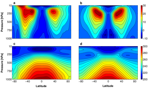
Figure 1.— The zonal mean zonal wind (m s^-1) (top), and zonal mean temperature distribution (K) (bottom) from Earth’s NCEP reanalysis data averaged over the years 1970-2012 (left) and the reference simulation (right).

2.1.2 Surface boundary layer

Our surface boundary-layer scheme is similar to that of Frierson et al. (2006). The lower boundary of the GCM is a uniform water covered slab, with an albedo of $\alpha=0.35$. A planetary boundary layer scheme with Monin-Obhukov surface fluxes (Obukhov, 1971), which depend on the stability of the boundary layer, links atmospheric dynamics to surface fluxes of momentum, latent heat, and sensible heat. The roughness length for momentum is $5\times 10^{-3}$, and for moisture and heat fluxes is $1\times 10^{-5}$ m, and an additive gustiness term of 1 m s^-1 in surface velocities comes to represent subgrid-scale wind fluctuations. These values yield energy fluxes and a climate similar to Earth’s in the aquaplanet setting of our simulations (Fig. 1). Our results are not very sensitive to the choice of these parameters.

The lower boundary is a “slab ocean”, comprising a vertically uniform layer of liquid water of depth $H$, here taken to be 1 m thick, with no dynamics and a horizontally varying temperature evolving as

$$c_{po}\rho_{0}H\frac{\partial T_{s}}{\partial t} = R_{s}\left(1-\alpha\right)-R_{u}-L_{e}E-S,$$ (11)

where $c_{po}=3989$ J kg^-1 K^-1 is the surface heat capacity, $\rho=1035$ kg m^-3 is the effective density of the slab ocean, $L_{e}=2.5\times 10^{6}$ J kg^-1 is the latent heat of vaporization and $R_{u}$ is the net upward longwave flux from the ocean surface. $E$ and $S$ and $\Sigma$ are the surface evaporative heat flux, sensible heat flux and surface stress respectively which are given by

$$E = \rho_{a}C\left|\mathbf{u}_{a}\right|\left(q_{a}-q_{s}^{*}\right),$$ (12)

$$S = \rho_{a}c_{p}C\left|\mathbf{u}_{a}\right|\left(T_{a}-T_{s}\right),$$ (13)

$$\mathbf{\Sigma} = C\rho_{a}\left|\mathbf{u}_{a}\right|\left|\mathbf{u}_{a}\right|,$$ (14)

where $\rho_{a},\mathbf{u}_{a},T_{a}$ and $q_{a}$ are the density, horizontal wind, temperature and humidity at the lowest atmospheric level. $q_{a}^{*}$ is the saturation specific humidity at the lowest model layer (see below), and $C$ is a drag coefficient which decays with height following Monin-Obhukov theory (Obukhov, 1971; Frierson et al., 2006). For further details see GFDL (2004). The neglect of horizontal mixing and heat transport in the ocean is a reasonable assumption in the Earth climate regime, since only one-third of Earth’s meridional heat transport occurs in the ocean, with the remaining two-thirds occurring in the atmosphere. Nevertheless, there may be some exoplanet regimes in which this assumption breaks down (e.g., Hu & Yang 2014).

Above the boundary layer, horizontal $\nabla^{8}$ hyperdiffusion in the vorticity, divergence, and temperature equations is the only frictional process. The hyperdiffusion coefficient is chosen to give a damping time scale of $12$ hrs at the smallest resolved scale.

2.1.3 Hydrological cycle

We include a hydrological cycle involving the evaporation, condensation, and transport of water vapor. Moisture is calculated at every grid point and depends on the surface evaporative fluxes and the convection giving the moisture equation

$$\frac{Dq}{Dt} = g\frac{\partial E}{\partial p}-\frac{Q_{c}}{L_{e}}.$$ (15)

A large-scale (grid-scale) condensation scheme ensures that the mean relative humidity in a grid cell does not exceed 100% (Frierson, 2007; O’Gorman & Schneider, 2008). Only the vapor-liquid phase change is considered, and the saturation vapor pressure $e_{s}$ is calculated from a simplified Clausius-Clapeyron relation given by

$$e_{s}\left(T\right) = e_{0}\exp\left[-\frac{L_{e}}{R}\left(\frac{1}{T}-\frac{1}{T_{0}}\right)\right],$$ (16)

where $R_{v}=461.5$ J kg^-1K^-1 is the gas constant for water vapor, $e_{0}=610.78$ Pa and $T_{0}=$273.16 K. The saturation specific humidity is then calculated by $q_{s}=\frac{R_{v}e_{s}}{R_{d}p}$. Moist convection is represented by a Betts-Miller like quasi-equilibrium convection scheme (Betts, 1986; Betts & Miller, 1986), relaxing temperatures toward a moist adiabat with a time scale of 2 hours, and water vapor toward a profile with fixed relative humidity of 70% relative to the moist adiabat, whenever a parcel lifted from the lowest model level is convectively unstable. Large-scale condensation removes water vapor from the atmosphere when the specific humidity on the grid scale exceeds the saturation.

2.2. Reference climate

Before presenting the dependence of the climate on the orbital and atmospheric parameters, we begin by presenting below the reference climate against which all experiments are compared. We choose this to be a climate similar to Earth’s climate, which to leading order is a well-understood regime, and allows us to check the validity of our model by comparing it to observations. Our strategy is to perform systematic parameter space sweeps all in reference to this single reference climate. With the parameter choice presented above the model reference climate is set to represent an Earth like annual-mean climate. Fig. 1 shows the zonally averaged temperature and wind fields for this reference climate (right), and the annually averaged climate for Earth from the National Centers for Environmental Prediction (NCEP) reanalysis data averaged over 40 years (1970-2010, left). Despite the simplicity of the model the resulting mean climate represents well Earth’s annual mean climate. The tropics are dominated by Hadley cells reaching nearly latitude $30^{\circ}$ with a generally weak westward zonal flow, and midlatitudes are dominated by an eastward jet streams with wind velocities reaching about $30$ m s^-1 at latitude $45^{\circ}$ and 200 hPa. Of course the model results are hemispherically symmetric, in contrast to the Earth data which varies considerably between hemispheres. In addition, our model does not have a seasonal cycle, which affects the climate despite not appearing directly in the annual averaged climate. Despite these differences, the choice of parameters given in section 2.1 yields a mean climate similar to observations. Fig. 3 (upper right) shows the surface temperature map resembling that of Earth’s observations with wave number five Rossby waves dominating the midlatitude climate.

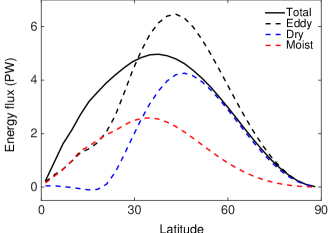
Figure 2.— The total (full) and eddy (dashed) poleward moist static energy flux (PW). The eddy flux is divided to its dry (blue) and moist (red) components.

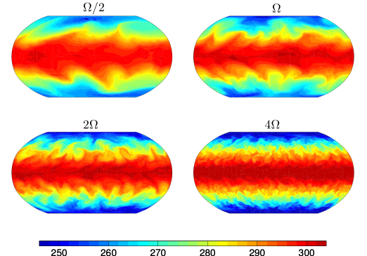
Figure 3.— Surface temperature (colorscale, in K) illustrating the dependence of temperature and eddy scale on rotation rate. Simulations have rotation rates ranging from half (upper left) to four times that of Earth (lower right). Baroclinic instabilities dominate the dynamics in mid- and high-latitudes, leading to baroclinic eddies whose length scales decrease with increasing planetary rotation rate.

A main focus of this paper will be on what controls the equator-to-pole temperature difference on terrestrial exoplanets. For Earth, if the planet had no atmospheric and oceanic dynamics and the planet were in pure radiative equilibrium, the equator-to-pole temperature difference would be much larger than the actual value (Hartmann, 1994). The existence of dynamics in the atmosphere, and particularly the fact that the atmosphere is turbulent, leads to a net poleward heat flux, which results in the cooling of the lower latitudes and heating of high latitudes, and therefore a much more equable climate than a planet in pure radiative equilibrium. This results in the reduction of the mean equator-to-pole temperature difference. The total heat transport can be described in terms of the moist static energy (MSE) defined as

$$m = c_{p}T+gz+L_{e}q,$$ (17)

where all symbols were defined in section 2.1. For Earth’s climate the global moist static energy flux is poleward in both hemispheres and peaks at about $5\times 10^{15}$ W in midlatitudes (Fig. 2). The total flux can be divided into a time mean component and a variation from the time mean coming from the turbulence in the atmosphere. If we divide the meridional velocity into a time mean denoted by an over-line and deviations from the time mean (eddies) with a prime so that $v=\overline{v}+v^{\prime}$, and do similarly for the moist static energy then

$$\overline{vm} = \overline{v}\,\overline{m}+\overline{v^{\prime}m^{\prime}}.$$ (18)

Fig. 2 shows the zonal averaged total flux ($\overline{vm}$) and the eddy flux ($\overline{v^{\prime}m^{\prime}}$), divided into the dry static energy component $\overline{v^{\prime}s^{\prime}}$, where $s=c_{p}T+gz$, and the latent energy component $L_{e}\overline{v^{\prime}q^{\prime}}$. It shows the dominance of the eddy term within the total flux (in midlatitudes it is even bigger since the mean component is negative), and the fact that the dry and moist components contribute roughly equally to this flux. For Earth, the moist component is more dominant in low latitudes and the dry component in high latitudes. This reflects the strong nonlinear dependence of the saturation vapor pressure on temperature (Eq. 16), meaning that warmer climates will have stronger heat transport due to latent heating (see section 3.2). Since the surface temperature is coupled to the atmosphere the radiation and evaporation also respond to the MSE transport giving important feedbacks to the steady state temperature through the Planck, evaporative and lapse rate feedbacks (e.g., Pithan & Mauritsen 2014).

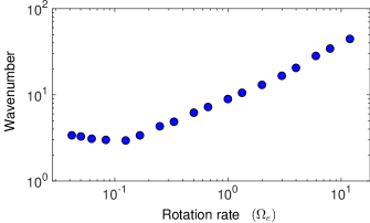
Figure 4.— The energy-containing wavenumber as function of the rotation rate of the planet, compared to Earth’s rotation rate ($\Omega_{e}$).

3. Results

3.1. Dependence on the rotation rate

We begin with a series of experiments where we vary the rotation rate of the planet (e.g., Williams & Holloway, 1982; del Genio & Suozzo, 1987; Williams, 1988; Navarra & Boccaletti, 2002; Schneider & Walker, 2006; Chemke & Kaspi, 2015). The main effect of increasing the rotation rate is that the eddy length scales decrease (we refer to eddies as the deviation from the time mean flow). This results from the fact that the primary source of extratropical eddies is from baroclinic instability (e.g., Pedlosky, 1987; Pierrehumbert & Swanson, 1995), and the dominant baroclinic length scale scales inversely with rotation rate (e.g., Schneider & Walker, 2006). This is illustrated in Fig. 3, which shows instantaneous snapshots of the surface temperature of experiments with the properties of the our reference climate, but where the rotation rate is varied between half and four times that of Earth. The waves in the temperature field are Rossby waves (e.g., Vallis, 2006), resulting from the latitudinal dependence of the Coriolis forces in the horizontal momentum equations (Eq. 1,2). The smaller eddies in the rapidly rotating models, demonstrated by the energy-containing wavenumber in Fig. 4, are less efficient in transporting MSE meridionally, leading to a greater equator-to-pole temperature difference for those cases. A similar dependence has been found in other studies as well (e.g., Schneider & Walker, 2006; Kaspi & Schneider, 2011, 2013).

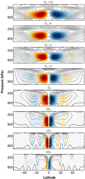
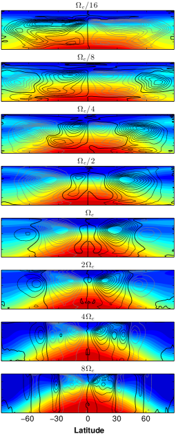
Figure 5.— Zonal-mean circulation for a sequence of idealized GCM experiments ranging from 1/16th to eight times the rotation rate of Earth from top to bottom, respectively. Left column: Thin black contours show zonal-mean zonal wind with a contour interval of 5 m s^-1, and the zero-wind contour is shown in a thick black contour. In color is the mean-meridional mass streamfunction, with blue denoting clockwise circulation and red denoting counterclockwise circulation. Maximum mass streamfunction values correspond to 8.7, 5.1, 4.2, 3, 1.9, 1.2, 0.6, 0.2 $\times 10^{11}$ kg s^-1, from top to bottom, respectively. Right column: colorscale shows zonal-mean temperature, with colorscale ranging between 210 K and 290 K. Contours show zonal-mean meridional eddy-momentum flux, $\overline{u^{\prime}v^{\prime}}$. Contour spacing grows from $9$ m² s^-2 in the slowly rotating cases to $1$ m² s^-2 in the fast rotating cases. Black and gray contours denote positive and negative values, respectively (implying northward and southward transport of eastward eddy momentum, respectively).

The strong dependence of the atmospheric circulation on rotation rate is because of the dominance of the Coriolis acceleration in the momentum balance. This can be quantified in terms of the Rossby number which is the ratio between the typical velocity and the rotation rate times a typical length scale $\frac{u}{\Omega L}$ (Pedlosky, 1987). Typically, away from the equator for Earth’s atmosphere and ocean the Rossby number is smaller than one, meaning that in Eq. (1–3), the leading order balance is geostrophic, and thus between the Coriolis and pressure forces in the horizontal momentum equations. However, planetary atmospheres are not necessarily in that regime (e.g., Showman et al., 2014). Solar system examples are Venus and Titan which have rotation rates of 243 days and 16 days respectively, and therefore are characterized by larger Rossby numbers. This is demonstrated in Fig. 5, where we show the zonal winds, temperature, meridional mass streamfunction, and meridional zonal-momentum fluxes ($\overline{u^{\prime}v^{\prime}}$) for cases of $1/16$, $1/8,$ $1/4$, $1/2,$ $1$, 2, 4 and 8 times the rotation rate of Earth. The mass streamfunction is defined as $\psi\left(\theta,p\right)=2\pi a\cos\theta\int v\left(\theta,p\right)dp/g$. Simulation results presented here and throughout the paper have been both zonally (longitudinally) and time averaged.

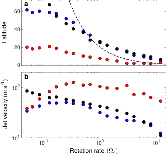
Figure 6.— (a) The latitude of the Hadley cell maximum (red), Hadley cell width (black) and the latitudinal location of the maximum jet. The dashed line shows the Hadley cell width following the axisymmetric theory of Held & Hou (1980). (b) The magnitude of the subtropical jet (blue), the magnitude of an angular momentum conserving wind ($u_{M}$) at the latitude of the maximal jet (red), and the strength of the Hadley Cell streamfunction (black) to the power of $2/5$.

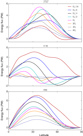
Figure 7.— The eddy (top), mean (middle) and total (bottom) poleward MSE flux as function of latitude for simulations with different planetary rotation rates.

As rotation rate is increased the Rossby number becomes smaller and more jets (regions of localized zonal velocity) develop (e.g., Williams & Holloway, 1982; Williams, 1988; Schneider & Walker, 2006; Chemke & Kaspi, 2015). These jets are generated by two distinct mechanisms, which we can categorize as thermally, and eddy, driven. In the former, the differential heating between low and high latitudes causes air to rise at the equator, flow poleward aloft, and sink at higher latitudes forming Hadley cells (colors on the left column of Fig. 5). Air flowing polewards within the upper branch of the Hadley cell moves closer to the axis of rotation of the planet, and therefore to conserve angular momentum it must develop eastward velocity (contours in the left side of Fig. 5). Within the Hadley cells meridional temperature differences are weak, creating a strong temperature gradient on the poleward side of the Hadley cell. For the cases of small Rossby number (rapidly rotating) geostrophy then implies that the atmosphere must be in thermal wind balance, meaning that

$$f\frac{\partial u}{\partial p} = \frac{R_{d}}{p}\frac{1}{a}\left(\frac{\partial T}{\partial\theta}\right)_{p},$$ (19)

thus that the vertical wind shear is proportional to the latitudinal temperature gradients along isobars. This then implies that the strong temperature gradient at the poleward side of the Hadley cell must be balanced by strong local wind shear, which then results in a local maxima of eastward velocity (Fig. 5). This jet is referred to as the subtropical jet (due to its location on Earth — at the edge of the Hadley cell), and is evident in the faster rotation cases in Fig. 5. For the slower rotation cases (Rossby number $\gtrsim$ 1), the eastward jets are a consequence of the conservation of angular momentum of poleward moving air in the upper branch of the Hadley cell, and therefore the jet magnitude is closer to that expected simply by conservation of angular momentum given by $u_{M}=\Omega a\frac{\sin^{2}\theta}{\cos\theta}$ (Held & Hou, 1980; Vallis, 2006). Figure 6 shows both the magnitude of the subtropical jet and the magnitude of $u_{M}$ for a series of simulations with different rotation rates ranging from $1/24$ to $12$ times the rotation rate of Earth. It shows that the slowly rotating cases develop stronger jets which are close to the angular momentum conserving value, while for the fast rotating cases the geostrophically balanced jets (Eq. 19) are much weaker than $u_{M}$. The strength of the subtropical jet scales nicely with the Hadley cell strength to the $2/5$ power following Held & Hou (1980), as shown in Fig. 6b.

The other type of jets — eddy driven jets — appear in the rapidly rotating cases. Here, breaking of Rossby waves in the extratropics results in eddy momentum flux convergence in the extratropics, and the formation of jets due to this convergence of momentum. This can be seen in Fig. 5 showing multiple zonal jets (left side) corresponding to areas where there is momentum flux convergence (Fig. 5, right side). The resulting jets from this mechanism have a more barotropic structure then the subtropical jets (Vallis, 2006). For the Earth rotation rate case the subtropical and eddy-driven jets appear almost merged in Fig. 5 (and Fig. 1, but are then clearly separable for the cases with faster rotation rates. The number of jets in each hemisphere is then related to the typical eddy length scale, and the inverse energy cascade length scales (Rhines, 1975, 1979; Chemke & Kaspi, 2015).

At slow rotation rates, the Hadley cells are nearly global, the subtropical jets reside at high latitude, and the equator-pole temperature difference is small (Fig. 5). The low-latitude meridional momentum flux is equatorward, leading to equatorial superrotation (eastward winds at the equator) in the upper troposphere (Mitchell & Vallis, 2010), qualitatively similar to that on Venus and Titan. At faster rotation rates, the Hadley cells and subtropical jets contract toward the equator, and simultaneously an extratropical zone, with eddy-driven jets, develops at high latitudes, and the equator-pole temperature difference is large. The low-latitude meridional momentum flux is poleward, resulting from the absorption of equatorward-propagating Rossby waves coming from the extratropics. It is also evident from Fig. 5 that as the rotation rate is increased the equator to pole temperature difference increases. This is a result of the combination of the facts that as rotation rate increases, the decreases in eddy length scale results in less eddy transport polewards, and that the slower rotation rate cases have large planetary scale Hadley cells which increase the heat transport by the mean meridional circulation.

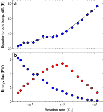
Figure 8.— (a) The equator-to-pole surface temperature difference as function of the rotation rate of the planet. (b) The maximum value of the poleward eddy heat transport (red), $\overline{v^{\prime}m^{\prime}}$, and mean transport (blue), $\overline{v}\,\overline{m}$, as function of the rotation rate of the planet. Fast rotation rate simulations are dominated by the decrease in eddy length scale with rotation rate resulting in less eddy heat transport poleward. Slower rotation rate experiments are dominated by large Hadley cells resulting in large mean heat transport and therefore smaller equator-to-pole temperature differences.

These two effects are shown in Fig. 7, which shows $\overline{v}\,\overline{m}$, $\overline{v^{\prime}m^{\prime}}$ and $\overline{vm}$ as function of latitude for different rotation rate cases. It shows that the turbulent heat flux $\overline{v^{\prime}m^{\prime}}$ has a nonmonotonic response to change of rotation rate. For slow rotation rates there is weak baroclinic instability and therefore the atmosphere is less turbulent resulting in weaker eddy heat transport ($\overline{v^{\prime}m^{\prime}}$), while for fast rotation rate the atmosphere is strongly baroclinically unstable but baroclinic zones are narrow and eddies are small resulting in weak $\overline{v^{\prime}m^{\prime}}$. Thus the maximum eddy poleward heat transport in these experiments is for rotation rates roughly similar to Earth’s (of course we should remember that our reference climate is tuned to Earth’s observed dynamics). On the other hand, the mean fluxes decrease monotonically with the increase of rotation rate (Fig. 7b), and this is because the Hadley cells become smaller for faster rotation (Fig. 6a). The majority of the contribution of the mean fluxes is at low latitudes (within the Hadley cell), and becomes a global heat transport only for the very slowly rotating cases where the Hadley cell becomes of the order of the size of the planet. In fact, for rotation rate cases faster than $1/4$ $\Omega_{e}$ the heat transport in the extratropics is negative because of the existence of Ferrel cells, and it dominates the overall mean transport ($\overline{v}\,\overline{m}$). Only for the extremely slow rotation planets when the Hadley cell is global does the extratropical heat transport by the mean become positive (Fig. 7b). An axisymmetric picture predicts that the Hadley cell width should be proportional to $\Omega^{-1}$ (Held & Hou, 1980), however this is complicated by the existence of eddies leading to more complex theories regarding where exactly the Hadley cells terminate (e.g., Schneider, 2006; Caballero, 2007; Levine & Schneider, 2011). The clear dependence of the Hadley cell width on the rotation rate is shown in Fig. 6a, with the $\Omega^{-1}$ line as a reference. In addition, warming of the extratropical surface temperature leads to additional radiative heating of the atmosphere creating therefore a positive feedback (Pithan & Mauritsen, 2014). In the steady state shown here all these processes have reached equilibrium.

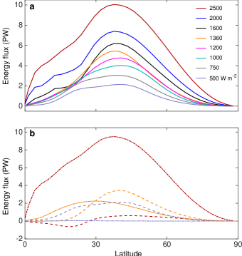
Figure 9.— (a) The eddy MSE transport for experiments with different stellar flux ranging from 500 to 2500 W m^-2 (b) Three cases from above (solar constant of 500, 1360 and 2500 W m^-2) showing the latent heat transport (dash-dot) and dry static energy transport (dash). This shows the strong nonlinear effect of water vapor on the MSE transport.

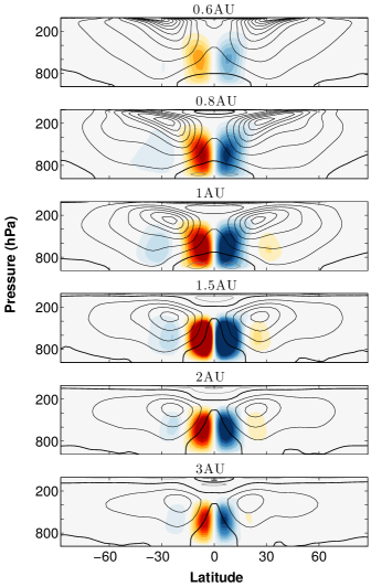
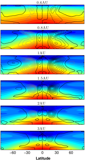
Figure 10.— Zonal-mean circulation for a sequence of idealized GCM experiments with stellar flux values of 3800, 2100, 1360, 607, 342 and 152 W m^-2, which correspond to a distance of 0.6, 0.8, 1, 1.5, 2 and 3 AU from their parent star (for Solar like luminosity) from top to bottom, respectively. Left column: Thin black contours show zonal-mean zonal wind with a contour interval of 5 m s^-1, and the zero-wind contour is shown in a thick black contour. In color is the mean-meridional mass streamfunction, with blue denoting clockwise circulation and red denoting counterclockwise circulation. Maximum and minimum streamfunction values correspond to $\pm 2.2\times 10^{11}$ kg s^-1 respectively, for all panels. Right column: colorscale shows zonal-mean temperature. Due to the large range of temperatures colorscale is different for each of the panels: maximum values are 354, 318, 301, 257, 222 and 183 K, and minimum values are 270, 233, 211, 173, 159 and 124 K from top to bottom, respectively. Contours show zonal-mean meridional eddy-momentum flux, $\overline{u^{\prime}v^{\prime}}$. Contour spacing is $3$ m² s^-2. Black and gray contours denote positive and negative values, respectively (implying northward and southward transport of eastward eddy momentum, respectively).

The sum of the eddy and the mean transports, giving the total heat transport, results in an overall larger heat transport for slower rotating planets; and therefore, planets with faster rotation to have larger equator-to-pole temperature differences (Fig. 8a). For the fast rotating cases this total is dominated by the eddies (even for the extreme fast rotation cases because the mean transport in those cases is negligible), and dominated by the mean transport for the less turbulent, slowly rotating cases. The transition between eddy- and mean-flow dominated transport occurs at a rotation rate of $0.2\Omega_{e}$ (location where red and blue points cross in Fig. 8b). Interestingly, however, the dependence of equator-pole temperature difference on rotation rate (i.e., the slope of the line in Fig. 8a) exhibits a clear kink at larger rotation rates of $\Omega_{e}$. This occurs because the dependence of eddy energy flux on rotation rate changes sign at $\Omega_{e}$. At rotation rates smaller than $\Omega_{e}$, eddies transport more energy when rotation rate is larger, but at rotation rates larger than $\Omega_{e}$, they transport less energy when rotation rate is larger (Fig. 8a, red points). By comparison, the mean flow transports less energy when rotation rate is larger across the entire parameter range explored (Fig. 8b, blue points). The sum of the red and blue points implies that the total energy transport is rather insensitive to rotation rate when $\Omega<\Omega_{e}$ but depends strongly on rotation when $\Omega>\Omega_{e}$. In turn, this leads to a relatively flat dependence of equator-pole temperature difference on rotation at low rotation rate but a strong dependence at high rotation rate, explaining the kink in Fig. 8a.

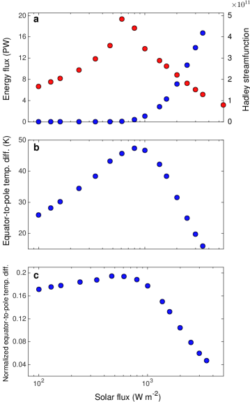
Figure 11.— (a) The maximum value of the Hadley cell mass streamfunction (red) and eddy latent heat flux (blue), $L\overline{v^{\prime}q^{\prime}}$, as function of the stellar heat flux. (b) The equator-to-pole surface temperature difference, and (c) the equator-to-pole surface temperature difference normalized by the mean surface temperature as function of the stellar heat flux. Strongly irradiated planets which are warmer and therefore have moister atmospheres, have a larger equator-to-pole MSE transport, which reduces the equator-to-pole temperature difference.

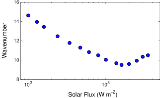
Figure 12.— The energy-containing wavenumber as function of the stellar flux.

3.2. Dependence on stellar flux

Next we look at the dependence of the circulation on the stellar flux. Since these experiments have no eccentricity and we treat the parent star as a constant point source of energy, these experiments are equivalent to varying the distance to the parent star. In our analysis we refer to both parameters interchangeably. As in the reference case which resembles Earth, the poleward heat transport for all cases with different solar heat fluxes is dominated by the eddy transport. Fig. 9a shows that planets with larger stellar flux have a larger poleward heat flux, which results in reduction of the equator-to-pole temperature difference (Fig. 10, Fig. 11b). The main reason for this increase in $\overline{v^{\prime}m^{\prime}}$ is the non-linear dependence of the Clausius-Clapeyron relation on temperature (Eq. 16). Warmer climates have greater atmospheric water vapor abundances, and therefore the relative effect of latent heating in the total MSE transport becomes more significant. Despite the important feedback between water vapor and optical thickness (e.g., Merlis & Schneider 2010), for simplicity we keep optical thickness fixed as in the reference climate.

Fig 9b shows the dry ($c_{p}\overline{v^{\prime}T^{\prime}}+g\overline{v^{\prime}z^{\prime}}$) and latent ($L\overline{v^{\prime}q^{\prime}}$) components of the eddy MSE transport for three cases with different solar fluxes. For the cooler case (500 W m^-2), the latent heat transport is very small compared to the dry component, while in the Earth case they are very similar in magnitude (with the latent component more dominant in the tropics and the dry component more dominant in the extratropics, Fig. 2). On the other hand in the very warm case (2500 W m^-2) the latent component becomes much larger than the dry component (Fig. 9b). The strong non-linearity is expressed in the fact that the difference in heating between the two sets of cases is similar (500, 1360 and 2000 W m^-2), but the increase in total heat flux has more than quadrupled.

The zonal mean climate for five cases ranging in distance from 0.6 to 2 AU (solar flux ranging between between 342 to 5470 W m^-2) is shown in Fig. 10. Obviously the closer-in planets are much warmer (Fig. 10, right side). The meridional mass streamfunction however shows nonmonotonic behavior (Fig. 10, left side). Planets far away from their parent star have less thermal forcing, and therefore Hadley and Ferrel cells get weaker as the stellar flux decreases. However, also as the planet becomes significantly warmer the strength of the Hadley and Ferrel cells becomes weaker. This is due to the nonlinear dependence of water vapor on temperature, where the increase in latent heating enables stronger MSE transport with a weaker circulation, resulting in weaker circulation cells in the warmer climates. The nonlinear increase in water vapor fluxes is also evident in Fig. 11a. For Earth like planets, the peak in the strength of the Hadley and Ferrel cells appears at about 1.5 AU (Fig. 10, left side). Quantitatively these results depend on the temperature dependence of the saturation vapor pressure, which can be different for planets with different atmospheric masses since then the ratio of latent to sensible heat will be different. However, despite the fact that the turning point may be different (Fig. 11a), we expect the general behavior to be similar to the results presented here.

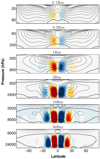
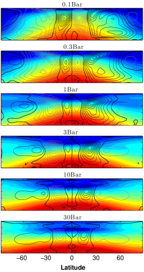
Figure 13.— Zonal-mean circulation for a sequence of idealized GCM experiments with surface pressure ranging from 0.1 to 30 bars from top to bottom, respectively. Left column: Thin black contours show zonal-mean zonal wind with a contour interval of 5 m s^-1. The zero-wind contour is shown in a thick black contour. In color is the mean-meridional mass streamfunction, with blue denoting clockwise circulation and red denoting counterclockwise circulation. Maximum and minimum streamfunction values correspond to $\pm 3\times 10^{11}$ kg s^-1, respectively for all panels. Right column: colorscale shows zonal-mean temperature, with colorscale ranging between 210 K and 290 K. Contours show zonal-mean meridional eddy-momentum flux, $\overline{u^{\prime}v^{\prime}}$. Contour spacing grows from $6$ m² s^-2 in the less massive cases to $1$ m² s^-2 in the more massive cases. Black and gray contours denote positive and negative values, respectively (implying northward and southward transport of eastward eddy momentum, respectively).

The domination of the moist component of the MSE flux results in that warmer planets have a smaller equator-to-pole temperature differences as long as moisture plays an important role in the transport as in the warm example in Fig. 9b. However, we find that once moisture is less important (cooler climates), this relation reverses and then as the distance to the star is increased the equator-to-pole temperature difference decreases again (Fig. 11b). Thus, despite the decrease in MSE flux with deceasing stellar flux (Fig. 9a), the equator-to-pole difference decreases leading to the nonmonotonic dependence in Fig. 11b. Mostly, this is due to the fact that for the cooler planets the mean temperature is smaller, and therefore even if the relative temperature difference would not have changed the absolute temperature difference between equator and pole is smaller. However, even the normalized equator-to-pole temperature difference (normalizing by the average surface temperature) shows a small decrease of temperature difference with reduction of solar flux (Fig. 11c), which is due to the increase in radiative time constant for the colder planets. Note that for these simulations the energy-containing wavenumber generally decreases with solar flux (Fig. 12). Therefore unlike the rotation rate experiments (section 3.1) where the eddy length scale decreased with rotation rate (Fig. 4), limiting the eddies ability to transport heat poleward and causing an increase in equator-to-pole temperature difference with rotation rate, here the reduction of eddy length scale does not result in increased equator-to-pole temperature difference. Thus, for the cooler planets, despite the decrease of eddy length scale with larger distance to the parent star, the equator-to-pole temperature difference is reduced.

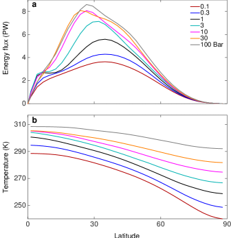
Figure 14.— (a) The poleward eddy MSE flux, and (b) the surface temperature as function of latitude for simulations with different surface pressure ranging from 0.1 bar to 100 bar. More massive atmospheres generally have a larger poleward MSE flux resulting in a reduced equator-to-pole temperature difference.

Figure 15.— (a) The maximum value of the meridional eddy MSE flux (blue); and the total vertical MSE flux (red) averaged between 400 and 600 hPa, as function of surface pressure. (b) The mean energy-containing wave number as function of surface pressure. (c) The equator-to-pole surface temperature difference as function of surface pressure. More massive atmospheres generally have a larger poleward MSE transport resulting in a reduced equator-to-pole temperature difference. The two competing effects of more MSE transport due to more atmospheric mass, and less MSE transport because of smaller and weaker eddies level out the equator-to-pole MSE transport in very massive atmospheres.

3.3. Dependence on atmospheric mass

Atmospheric masses can vary considerably based on the planetary composition and history. Even in our close neighbors in the solar system atmospheric masses vary by orders of magnitude from an atmosphere of $92$ bars on Venus, to an atmosphere of $0.006$ bars on Mars. The other terrestrial type atmosphere in the solar system, that of Titan, has an atmospheric surface pressure similar to Earth of $1.5$ bar. In this section we experiment with the atmospheric mass of the planet, by keeping all other parameters constant as in our reference climate, and varying only surface pressure. We use no convection scheme and do not vary optical thickness despite increasing atmospheric mass, to allow an even comparison between the simulations. Fig. 13 shows that as the atmospheric mass is increased the meridional cells of mass streamfunction become stronger and narrower, resulting also in the subtropical jet being closer to the equator. Note that the mass streamfunction in Fig. 13 is integrated over pressure, meaning that for the case of these simulations the increase in streamfunction strength does not necessarily coincide with stronger wind speeds. In fact, here as surface pressure is increased the Hadley and Ferrel cells have weaker velocities despite the increase in of the mass streamfunction. Eddy momentum flux convergence is aligned with the jet location and also becomes closer to the equator and weaker with increasing atmospheric mass. Note that the contour interval of $\overline{u^{\prime}v^{\prime}}$ decreases with atmospheric mass in Fig. 13.

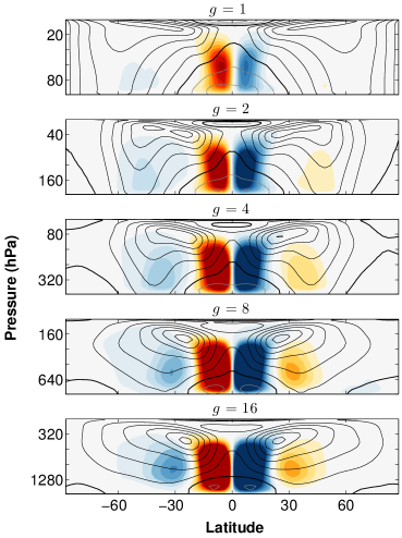
Figure 16.— Zonal-mean circulation for a sequence of idealized GCM experiments ranging in mean planetary density from 562 kg m^-3 to 7,874 kg m^-3 (corresponding to surface gravity ranging from 1 m s^-2 to 16 m s^-2). Left column: Thin black contours show zonal-mean zonal wind with a contour interval of 5 m s^-1, and the zero-wind contour is shown in a thick black contour. In color is the mean-meridional mass streamfunction, with blue denoting clockwise circulation and orange denoting counterclockwise circulation. Maximum and minimum streamfunction values grow with the gravity, and thus correspond to $\pm\left(1,2,4,8,16\right)\times 10^{10}$ kg s^-1, from top to bottom respectively. Right column: colorscale shows zonal-mean temperature, with colorscale ranging between 210 K and 290 K. Contours show zonal-mean meridional eddy-momentum flux, $\overline{u^{\prime}v^{\prime}}$. Contour spacing is $5$ m² s^-2. Black and gray contours denote positive and negative values, respectively (implying northward and southward flux of eastward eddy momentum, respectively).

Planets with more massive atmospheres also have stronger equator-to-pole MSE flux (Fig. 14a), which reduces the equator-to-pole temperature difference (Fig. 13 right side), and therefore the jet strength. In all cases the mass flux is dominated by the eddy component (as in the Earth case in Fig. 2), and the increase in MSE flux follows monotonically with the increase in atmospheric mass. This increase is mostly due to the increase in pressure (as the flux is vertically integrated over the atmosphere), and not due to the increase in the eddy correlations themselves ($\overline{v^{\prime}m^{\prime}}$) which actually decrease with atmospheric mass. The increase in MSE flux with atmospheric mass becomes more gradual beyond $10$ bars, likely because of the strong decrease in eddy length scale (Fig. 15b) for the extremely massive atmospheres. Thus the two competing effects of more efficient energy transport due to more atmospheric mass, and less efficient transport because of smaller eddies level out the equator-to-pole heat transport in very massive atmospheres. Nonetheless, the general trend of smaller equator-to-pole temperature differences with increasing atmospheric mass is obvious in Fig. 13 (right column), 14b, and 15c.

Fig. 14b shows that as atmospheric mass increases surface temperatures increases as well. This is a consequence of the fact that although horizontal heat transport increases with increasing atmospheric mass, vertical heat transport reduces in magnitude. This is demonstrated in Fig. 15a showing the total vertical MSE transport in the mid atmosphere (averaged between 400 and 600 hPa). Thus, despite the increase in the strength of the mass streamfunction, when integrated globally more massive atmospheres have less vertical heat transport, which results in the surfaces accumulating more heat (the optical thickness in these simulations depends only on $\sigma$ and therefore is equally distributed in height in all simulations). These differences are larger in midlatitudes than in the tropics since at midlatitudes the eddies play a larger role in the heat transport. This results in the fact that more massive atmospheres have larger extratropical lapse rates, which acts to destabilize the atmosphere. However, this increase of horizontal heat fluxes with atmospheric mass has the opposite effect (thus stabilizing the atmosphere), and is more dominant in our simulations, resulting in weaker eddy momentum fluxes and weaker jets as can be seen in Fig. 13.

3.4. Dependence on planetary mean density

Terrestrial type exoplanets likely span a wide range of mean densities ranging from ice-rich planets to heavy planets composed primarily of rock and iron. Here we explore the effect of varying the planetary mean density between the extremes of a relatively light ice-planet (1000 kg m^-3), to that of a heavy iron-planet (7,874 kg m^-3), while keeping the atmospheric mass constant. Thus, in these simulations the planet radius is kept fixed to that of Earth, and we also keep Earth’s atmospheric mass by varying the surface pressure hydrostatically given the varying surface gravity, where $g=\frac{4\pi}{3}G\rho$ (Fig. 17). Fig. 16 shows that Hadley and Ferrel cell strength increases with the gravity coefficient (note that the color scale changes between the panels). For the Hadley cell case the increase in width and strength is consistent with Held & Hou (1980) suggesting a $g^{1/2}$ increase in Hadley cell width and $g^{3/2}$ in Hadley cell intensity. In our simulations, despite showing the same trends, the increase in Hadley cell width and intensity is more modest likely due to the role of eddies. Concurrently, the midlatitude jets become more subtropical in nature (thus more baroclinic and closer to the edge of the Hadley cell). In the water-density planet the midlatitude jets are mainly eddy driven, weaker and more barotropic, while in the denser planets due to the dominance of the Hadley cell, and despite the strengthening of the eddies, the jets peak near the edge of the Hadley cells. On the other hand, the increase in Ferrel-cell strength is likely due to stronger baroclinic instability in midlatitudes (see below).

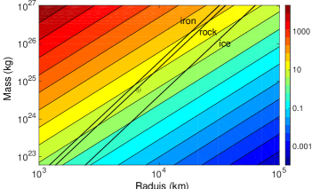
Figure 17.— The surface gravity (colorscale, $\rm m\,s^{-2}$) as function of planetary mass and radius. Black lines denote planets with a mean density of ice (1000 kg m^-3), rock (5520 kg m^-3) and iron (7,874 kg m^-3). The $\oplus$ symbol denotes the location of Earth in this phase space.

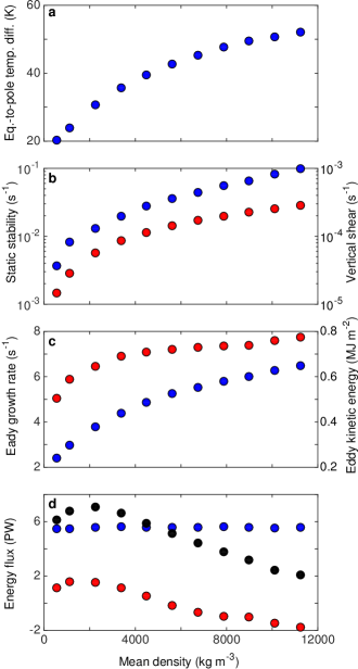
Figure 18.— (a) The equator-to-pole surface temperature difference as function of the mean density of the planet ranging between density of an ice-planet to that of a heavy iron-planet (Fig. 17). (b) Static stability (red), and vertical wind shear (blue) as function of the mean density of the planet. (c) Eady growth rate (Eq. 20, blue), and eddy kinetic energy (red). (d) Eddy MSE flux (blue), mean MSE flux (red) and total MSE flux (black) as function of the mean planetary density.

Unlike the rotation and atmospheric-mass experiments (sections 3.1,3.3), here the increased Hadley cell strength also results in an increase in equator-to-pole temperature differences (Fig. 16, right side), which shows roughly a tripling of the equator-to-pole surface temperature between the ice-density planet and the iron-density planet (Fig. 18a). The reason for this variation is that as the mean density increases, so do the buoyancy frequency and vertical shear which affect the Eady growth rate

$$\sigma\sim\frac{\Omega\sin\theta}{N}\frac{\partial u}{\partial z},$$ (20)

representing the growth rate of baroclinic eddies in the atmosphere (Eady, 1949; Lindzen & Farrell, 1980). The static stability and vertical shear exert opposite effects on the Eady growth rate and both depend on gravity. The static stability, $N^{2}=\frac{g}{\Theta}\frac{\partial\Theta}{\partial z}$, has a dependence on gravity both because of the direct dependence on gravity and the fact that the vertical gradient of potential temperature becomes larger for larger mass (again, because of the reduction of the vertical eddy heat flux). The vertical shear has a linear dependence since for a similar forcing by a temperature gradient thermal wind implies that the vertical shear will grow linearly with gravity (Eq. 19). Taking into account both dependencies (Fig. 18b), we find that heavier planets will have a larger Eady growth rate implying stronger baroclinic eddies and eddy kinetic energy (Fig. 18c). However, this does not cause stronger eddy heat fluxes (Fig. 18d, blue points), but rather the larger eddy activity in midlatitudes strengthens the eddy-driven Ferrel cell that drives a stronger equatorward mean circulation (Fig. 18d, red points) that weakens the overall poleward heat transport (Fig. 18d, black points). The reduced overall poleward heat transport then results in an increased equator-to-pole temperature difference (Fig. 18a). The heavier planets therefore have stronger Ferrel cells and eddies in the extratropics, which is also evident when looking at the strength of the eddy kinetic energy, $\frac{1}{2g}\int\left(u^{\prime 2}+v^{\prime 2}\right)dp$, integrated over the troposphere (Fig. 18c). On the other hand, if atmospheric surface pressure, rather than atmospheric mass, is held constant while the gravity is varying (not shown), then the simulations would resemble those of varying atmospheric mass where the equator-to-pole temperature differences decreases with increasing the gravity.

Figure 19.— (a) The eddy moist (solid) and dry (dashed) static energy fluxes as function of latitude for three cases of different optical thicknesses, which correspond to a mean surface temperature of 254, 286 and 318 K. (b) The equator-to-pole surface temperature difference as function of the mean surface temperature of the planet, corresponding to experiments with 0.1 to 15 times the optical thickness of the reference case, which correspond to mean surface temperatures of $253$ K to $319$ K, respectively.

3.5. Dependence on optical thickness

In all previous sections optical thickness (Eq. 8) has been kept fixed, set to the parameters that give an Earth-like climate in the reference simulation (Fig. 1). Increasing the optical thickness while keeping other parameters fixed (including atmospheric mass) results in an atmosphere that absorbs more of the emitted longwave radiation and therefore is warmer. How this effects eddy momentum transport in the atmosphere and the equator-to-pole temperature difference is less straight forward; we explore this issue here. Over this series of simulations we increase $\tau_{p}$ and $\tau_{e}$ (Eq. 8) by the same factor, thus increasing the optical thickness linearly over all latitudes. In the series of experiments presented here the optical thickness was varied between $0.1$ to $15$ times the reference case, which corresponds to mean surface temperatures of $253$ K to 319 K respectively. In resemblance to the case of varying the stellar flux (section 3.2), the results are dominated by the nonlinear response of temperature to the atmospheric water-vapor abundance. For the cases with low optical thickness the atmosphere is cold resulting in dry static energy dominating the moist static energy fluxes (Fig. 19a), and thus less overall poleward heat transport resulting in a large equator-to-pole temperature difference (Fig. 19b). As the optical depth is increased the moist component of the MSE becomes larger resulting in stronger MSE transport and therefore smaller equator-to-pole temperature differences. However, unlike the stellar flux experiments the monotonic increase does not happen over all latitudes resulting that at midlatitudes the colder simulation have stronger flux. This requires further investigation. Note that in our simple model as optical thickness does not vary with the amount of water vapor, this model does not allow for a runaway effect as perhaps relevant to Venus.

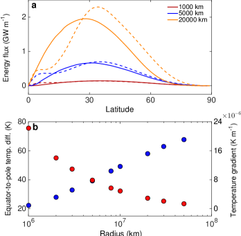
Figure 20.— (a) The eddy moist (solid) and dry (dashed) static energy fluxes as function of latitude for three cases with different planetary radius of 1000 km, 5000 km and 20000 km (b) The equator-to-pole surface temperature difference (blue) and mean equator-to-pole surface temperature gradient (red) as function of the planetary radius.

3.6. Dependence on radius

In this set of experiments we keep the planetary mean density constant at the density of Earth (5520 kg m^-3), and vary the radius and correspondingly the mass and surface gravity of the planet (along the “rock” line in Fig. 17). If gravity would not have been changing then reducing the radius of the planet has a similar effect to increasing the rotation rate, since the Rossby number becomes smaller ($u/\Omega L$), where $L$ is the typical length scale. However, for a rocky planet changing the radius, results in a change of mass and surface gravity. Again, in this experiment we keep the mass of the atmosphere (per unit area) constant by consistently varying the surface pressure. Fig. 20 shows that larger planets have a smaller mean equator-to-pole temperature gradient due to the MSE transport increasing with planet size (in Fig. 20a MSE flux is normalized by planetary radius). For all simulations the MSE fluxes, in similar to the reference case, are dominated by the eddy fluxes, with the mean contributing negatively in midlatitude (as in Fig. 2). Similar to increasing the rotation rate of the planet (section 3.1), as the planet size is increased, the typical eddy length scale becomes smaller compared to the size of the planet and therefore is less efficient in heat transport. This results in a larger equator-to-pole temperature difference (Fig. 20b.

4. Discussion and conclusion

To date, nearly a hundred terrestrial exoplanets have been identified, and this number is expected to grow significantly over the next few years as more Earth-sized and sub-Earth-sized planets are discovered. These planets span a wide range of orbital parameters and incident stellar fluxes, and they likely also span a wide range of climatic regimes. In this work, we have attempted to characterize the basic features of the general circulation of these atmospheres, focusing on planets that are far enough away from their parent star so that they are not tidally locked, and therefore to leading order, like Earth, have a zonally symmetric climate. In this sense this study is different than many recent studies focusing on the atmospheric dynamics of tidally locked terrestrial exoplanets (e.g., Joshi et al., 1997; Joshi, 2003; Merlis & Schneider, 2010; Heng & Vogt, 2011; Wordsworth et al., 2011; Selsis et al., 2011; Yang et al., 2013, 2014; Hu & Yang, 2014; Heng & Showman, 2015; Showman et al., 2015). For simplicity we have attempted to keep the model configuration as simple as possible (aquaplanet, no seasons, no ice, simplified radiation), and we presented several series of numerical GCM simulations experiments exploring one parameter at a time. Being one of the first studies that are addressing such planetary regimes, we have attempted to address only the basic features of these diverse planetary atmospheres. We therefore focus on the equator-to-pole temperature difference, and the size and intensity of the Hadley cells, Ferrel cells and extratropical jet streams. We focus on six unique systematic experiments which contain in our view some of the more interesting characteristics of the planetary atmospheres: rotation rate, stellar flux, atmospheric mass, surface gravity, optical thickness and planetary radius. Of course, these six encompass only a small subset of possible explorable parameters. An alternate approach would be to nondimensionalize the equations and vary only the nondimensional parameters. However, in order to give better intuition we decided to present our integrations using the real physical parameters.

The key results for the six sets of simulations presented in section 3 are given below:

• Planets with faster rotation rates are characterized by smaller and weaker Hadley cells, and smaller eddy length scales. This results in a larger equator-to-pole temperature difference, and weaker jets. The number of jets grows with rotation rate. Slowly rotating planets will have an equatorial eddy momentum flux convergence resulting in superrotation (e.g., Venus, Titan).

• The stellar flux has a nonmonotonic response in most aspects we have examined, due to the strong nonlinear dependence of water vapor abundance on temperature. Warmer and closer planets will have smaller equator-to-pole temperature differences due to enhanced eddy MSE transport due to the latent heat component, which increases significantly with temperature. However, planets which are far enough from the their parent star, so that for their abundance of water vapor the atmospheres are dry, will also have smaller equator-to-pole temperature differences due to the overall lower temperatures and larger radiative time scales. Hadley and Ferrel cells exhibit the same nonmonotonic behavior.

• Planets with larger atmospheric masses, generally have larger horizontal fluxes but lower vertical fluxes, resulting in reduced equator-to-pole temperature differences, and higher surface temperatures. Hadley and Ferrel cells increase in strength with atmospheric mass due to the increased mass transport.

• Planets with larger mean densities and therefore larger surface gravity have stronger Hadley and Ferrel cells. For these cases despite the growth of eddy energy with surface gravity, the main controller of the extratropical temperature is the strengthening of the Ferrel cells, and therefore the equator-to-pole temperature difference increases with mean planetary density.

• Planets with larger optical thickness are warmer across all latitudes, and the equator-to-pole temperature difference decreases with the increase of optical thickness due to enhanced poleward eddy MSE transport (mainly because of increased latent heat transport) in the warmer climates.

• Planets with larger radii and consequently larger gravity show a decrease in equator-to-pole temperature gradient with increasing radius due to enhanced poleward eddy MSE transport. However, despite the reduction in temperature gradients, this effect does not compensate for the increase in distance between the equator and the pole, and therefore overall the equator-to-pole temperature difference increases.

• The dependence of the equator-to-pole temperature difference on rotation rate, atmospheric mass, and other parameters implies that dynamics may exert a significant effect on global-mean climate feedbacks such as the conditions under which a planet transitions into a globally frozen, ”Snowball Earth” state. Thus, our results imply that the dynamics influences planetary habitability, including the width of the classical habitable zone.

A key result, which has important implication for the habitability of these planets, is the equator-to-pole temperature difference response to the variation in orbital and atmospheric parameters. As we have discussed, large-scale atmospheric turbulence attempts to homogenize latitudinal temperature differences, mainly through poleward transport of moist static energy. In the simulations presented here, we find that the equator-to-pole temperature difference increases for larger rotation rates, planets with larger surface gravity (density) and larger radius planets, while the equator-to-pole temperature difference decreases with atmospheric mass, larger optical thickness and for cooler or warmer planets (depending on water vapor). Varying the distance to the parent star has a nonmonotonic response in the equator-to-pole temperature difference due to the nonlinear dependence of water vapor on temperature. Despite the fact that these results have been obtained in respect to an Earth like reference atmosphere, the combination of experiments represent the general trends we expect to find in any atmosphere. Known examples which are consistent with our results are the terrestrial type atmospheres of Venus, Mars and Titan. The slow rotating Venus has a very small equator-to-pole temperature difference and strong jets, despite having a massive atmosphere (92 bars). Titan has a large global Hadley cells due to its slow rotation, and Mars has a similar rotation rate to Earth but an atmosphere of only 0.006 bar and therefore has large equator-to-pole temperature differences.

Moreover, this analysis has implications for the understanding of solar system planetary atmospheres as well. The observed equator-to-pole temperature difference on Venus is only a few degrees Kelvin (Prinn & Fegley, 1987), and it is unclear if this is because of Venus’s slow rotation or its massive atmosphere with a resulting long radiative time scale. Extrapolating from our results for varying atmospheric mass and rotation rate, which both give smaller equator-to-pole temperature differences for a 92 bar atmosphere rotating at $\sim 0.004\Omega_{e}$, respectively (Figs. 8a, 15b), implies that both slow rotation and a massive atmosphere are necessary for such a small equator-to-pole temperature difference.

As more detailed exoplanet observations become available, we will be able to provide more constraints to these planetary atmospheres to better constrain the models. This paper provides a first attempt to characterize these atmospheres, focusing on the main drivers of the atmospheric circulation and the resulting climate. Developing this mechanistic understanding of what controls the climate, will allow to better provide constraints on what influences habitability on these planets.

References

- Adams et al. (2008) Adams, E. R., Seager, S., & Elkins-Tanton, L. 2008, Astrophys. J., 673, 1160
- Aharonson et al. (2009) Aharonson, O., Hayes, A. G., Lunine, J. I., et al. 2009, Nature Geoscience, 2, 851
- Ballard et al. (2013) Ballard, S., Charbonneau, D., Fressin, F., et al. 2013, Astrophys. J., 773, 98
- Barclay et al. (2013) Barclay, T., Rowe, J. F., Lissauer, J. J., et al. 2013, Nature, 494, 452
- Batalha et al. (2011) Batalha, N. M., Borucki, W. J., Bryson, S. T., et al. 2011, Astrophys. J., 729, 27
- Bean et al. (2010) Bean, J. L., Miller-Ricci Kempton, E., & Homeier, D. 2010, Nature, 468, 669
- Bean et al. (2011) Bean, J. L., Désert, J.-M., Kabath, P., et al. 2011, Astrophys. J., 743, 92
- Berta et al. (2012) Berta, Z. K., Charbonneau, D., Désert, J.-M., et al. 2012, Astrophys. J., 747, 35
- Betts (1986) Betts, A. K. 1986, Q. J. R. Meteorol. Soc., 112, 677
- Betts & Miller (1986) Betts, A. K., & Miller, M. J. 1986, Q. J. R. Meteorol. Soc., 112, 693
- Bohren & Albrecht (1998) Bohren, C. F., & Albrecht, B. A. 1998, Atmospheric thermodynamics (Oxford University Press)
- Borucki et al. (2011) Borucki, W. J., Koch, D. G., Basri, G., et al. 2011, Astrophys. J., 736, 19
- Borucki et al. (2013) Borucki, W. J., Agol, E., Fressin, F., et al. 2013, Science, 340, 587
- Bourke (1974) Bourke, W. 1974, Mon. Weath. Rev., 102, 687
- Caballero (2007) Caballero, R. 2007, Geophys. Res. Lett., 34, 22705
- Charbonneau et al. (2009) Charbonneau, D., Berta, Z. K., Irwin, J., et al. 2009, Nature, 462, 891
- Chemke & Kaspi (2015) Chemke, R., & Kaspi, Y. 2015, J. Atmos. Sci., doi:10.1175/JAS-D-15-0007.1, in press
- de Mooij et al. (2012) de Mooij, E. J. W., Brogi, M., de Kok, R. J., et al. 2012, Astron. and Astrophys., 538, A46
- del Genio & Suozzo (1987) del Genio, A. D., & Suozzo, R. J. 1987, J. Atmos. Sci., 44, 973
- Désert et al. (2011) Désert, J.-M., Bean, J., Miller-Ricci Kempton, E., et al. 2011, Astrophys. J. Let., 731, L40
- Dressing & Charbonneau (2013) Dressing, C. D., & Charbonneau, D. 2013, Astrophys. J., 767, 95
- Eady (1949) Eady, E. T. 1949, Tellus, 1, 33
- Forget & Leconte (2014) Forget, F., & Leconte, J. 2014, Royal Society of London Philosophical Transactions Series A, 372, 30084
- Fortney et al. (2013) Fortney, J. J., Mordasini, C., Nettelmann, N., et al. 2013, Astrophys. J., 775, 80
- Fraine et al. (2013) Fraine, J. D., Deming, D., Gillon, M., et al. 2013, Astrophys. J., 765, 127
- Fressin et al. (2012) Fressin, F., Torres, G., Rowe, J. F., et al. 2012, Nature, 482, 195
- Frierson (2007) Frierson, D. M. W. 2007, J. Atmos. Sci., 64, 1959
- Frierson et al. (2006) Frierson, D. M. W., Held, I. M., & Zurita-Gotor, P. 2006, J. Atmos. Sci., 63, 2548
- GFDL (2004) GFDL. 2004, J. Climate, 17, 4641
- Gillon et al. (2014) Gillon, M., Demory, B.-O., Madhusudhan, N., et al. 2014, Astron. and Astrophys., 563, A21
- Hartmann (1994) Hartmann, D. L. 1994, Global Physical Climatology (Academic P.)
- Held (1982) Held, I. M. 1982, J. Atmos. Sci., 39, 412
- Held & Hou (1980) Held, I. M., & Hou, A. Y. 1980, J. Atmos. Sci., 37, 515
- Held & Suarez (1994) Held, I. M., & Suarez, M. J. 1994, Bull. Am. Meteor. Soc., 75, 1825
- Heng & Showman (2015) Heng, K., & Showman, A. P. 2015, Ann. Rev. Earth Plan. Sci., in press
- Heng & Vogt (2011) Heng, K., & Vogt, S. S. 2011, Mon. Not. Roy. Astro. Soc., 415, 2145
- Hu & Yang (2014) Hu, Y., & Yang, J. 2014, Proc. Natl. Acad. Sci. U.S.A., 111, 629
- Joshi (2003) Joshi, M. 2003, Astrobiology, 3, 415
- Joshi et al. (1997) Joshi, M. M., Haberle, R. M., & Reynolds, R. T. 1997, Icarus, 129, 450
- Kaspi & Schneider (2011) Kaspi, Y., & Schneider, T. 2011, J. Atmos. Sci., 68, 2459
- Kaspi & Schneider (2013) —. 2013, J. Atmos. Sci., 70, 2596
- Kreidberg et al. (2014) Kreidberg, L., Bean, J. L., Désert, J.-M., et al. 2014, Nature, 505, 69
- Leconte et al. (2013) Leconte, J., Forget, F., Charnay, B., et al. 2013, Astron. and Astrophys., 554, A69
- Léger et al. (2004) Léger, A., Selsis, F., Sotin, C., et al. 2004, Icarus, 169, 499
- Léger et al. (2011) Léger, A., Grasset, O., Fegley, B., et al. 2011, Icarus, 213, 1
- Levine & Schneider (2011) Levine, X. J., & Schneider, T. 2011, J. Atmos. Sci., 68, 769
- Lindzen & Farrell (1980) Lindzen, R. S., & Farrell, B. 1980, J. Atmos. Sci., 37, 1648
- Lorenz (1967) Lorenz, E. N. 1967, The Nature and Theory of the General Circulation of the Atmosphere (World Meteorological Organization)
- Merlis & Schneider (2010) Merlis, T. M., & Schneider, T. 2010, J. Adv. Mod. Earth Sys., 2, 13
- Mitchell et al. (2006) Mitchell, J. L., Pierrehumbert, R. T., Frierson, D. M. W., & Caballero, R. 2006, Proc. Natl. Acad. Sci. U.S.A., 103, 18421
- Mitchell & Vallis (2010) Mitchell, J. L., & Vallis, G. K. 2010, J. Geophys. Res., 115, 12008
- Muirhead et al. (2012) Muirhead, P. S., Hamren, K., Schlawin, E., et al. 2012, Astrophys. J. Let., 750, L37
- Navarra & Boccaletti (2002) Navarra, A., & Boccaletti, G. 2002, Clim. Dyn., 19, 467
- Nettelmann et al. (2011) Nettelmann, N., Fortney, J. J., Kramm, U., & Redmer, R. 2011, Astrophys. J., 733, 2
- Obukhov (1971) Obukhov, A. M. 1971, Boundary-Layer Meteorology, 2, 7
- O’Gorman & Schneider (2008) O’Gorman, P. A., & Schneider, T. 2008, J. Climate, 21, 3815
- Pedlosky (1987) Pedlosky, J. 1987, Geophysical Fluid Dynamics (Spinger)
- Pierrehumbert et al. (2011) Pierrehumbert, R. T., Abbot, D. S., Voigt, A., & Koll, D. 2011, Ann. Rev. Earth Plan. Sci., 39, 417
- Pierrehumbert & Swanson (1995) Pierrehumbert, R. T., & Swanson, K. L. 1995, Ann. Rev. Fluid Mech., 27, 419
- Pithan & Mauritsen (2014) Pithan, F., & Mauritsen, T. 2014, Nature Geoscience, 7, 181
- Prinn & Fegley (1987) Prinn, R. G., & Fegley, B. 1987, Ann. Rev. Earth Plan. Sci., 15, 171
- Quintana et al. (2014) Quintana, E. V., Barclay, T., Raymond, S. N., et al. 2014, Science, 344, 277
- Rhines (1975) Rhines, P. B. 1975, J. Fluid Mech., 69, 417
- Rhines (1979) —. 1979, Ann. Rev. Fluid Mech., 11, 401
- Rogers et al. (2011) Rogers, L. A., Bodenheimer, P., Lissauer, J. J., & Seager, S. 2011, Astrophys. J., 738, 59
- Schneider (2006) Schneider, T. 2006, Ann. Rev. Earth Plan. Sci., 34, 655
- Schneider et al. (2012) Schneider, T., Graves, S. D. B., Schaller, E. L., & Brown, M. E. 2012, Nature, 481, 58
- Schneider & Walker (2006) Schneider, T., & Walker, C. C. 2006, J. Atmos. Sci., 63, 1569
- Selsis et al. (2011) Selsis, F., Wordsworth, R. D., & Forget, F. 2011, Astron. and Astrophys., 532, A1
- Showman et al. (2015) Showman, A. P., Lewis, N. K., & Fortney, J. J. 2015, Astrophys. J., 801, 95
- Showman et al. (2014) Showman, A. P., Wordsworth, R. D., Merlis, T. M., & Kaspi, Y. 2014, Atmospheric Circulation of Terrestrial Exoplanets (The University of Arizona Press), 277–326
- Sinukoff et al. (2013) Sinukoff, E., Fulton, B., Scuderi, L., & Gaidos, E. 2013, Space Sci. Rev.
- Teske et al. (2013) Teske, J. K., Turner, J. D., Mueller, M., & Griffith, C. A. 2013, Mon. Not. Roy. Astro. Soc., 431, 1669
- Valencia et al. (2007) Valencia, D., Sasselov, D. D., & O’Connell, R. J. 2007, Astrophys. J., 656, 545
- Vallis (2006) Vallis, G. K. 2006, Atmospheric and Oceanic Fluid Dynamics (pp. 770. Cambridge University Press.)
- Voigt et al. (2011) Voigt, A., Abbot, D. S., Pierrehumbert, R. T., & Marotzke, J. 2011, Clim. of the Past, 7, 249
- Williams (1988) Williams, G. P. 1988, Clim. Dyn., 2, 205
- Williams & Holloway (1982) Williams, G. P., & Holloway, J. L. 1982, Nature, 297, 295
- Wordsworth & Pierrehumbert (2013) Wordsworth, R., & Pierrehumbert, R. 2013, Science, 339, 64
- Wordsworth et al. (2011) Wordsworth, R. D., Forget, F., Selsis, F., et al. 2011, Astrophys. J. Let., 733, L48
- Yang et al. (2014) Yang, J., Boué, G., Fabrycky, D. C., & Abbot, D. S. 2014, Astrophys. J. Let., 787, L2
- Yang et al. (2013) Yang, J., Cowan, N. B., & Abbot, D. S. 2013, Astrophys. J. Let., 771, L45