Maximizing Protein Translation Rate in the Nonhomogeneous Ribosome Flow Model: A Convex Optimization Approach

Abstract

Translation is an important stage in gene expression. During this stage, macro-molecules called ribosomes travel along the mRNA strand linking amino-acids together in a specific order to create a functioning protein.

An important question, related to many biomedical disciplines, is how to maximize protein production. Indeed, translation is known to consume most of the cell’s energy and it is natural to assume that evolution shaped this process so that it maximizes the protein production rate. If this is indeed so then one can estimate various parameters of the translation machinery by solving an appropriate mathematical optimization problem. The same problem also arises in the context of synthetic biology, namely, re-engineer heterologous genes in order to maximize their translation rate in a host organism.

We consider the problem of maximizing the protein production rate using a computational model for translation-elongation called the ribosome flow model (RFM). This model describes the flow of the ribosomes along an mRNA chain of length $n$ using a set of $n$ first-order nonlinear ordinary differential equations. It also includes $n+1$ positive parameters: the ribosomal initiation rate into the mRNA chain, and $n$ elongation rates along the chain sites.

We show that the steady-state translation rate in the RFM is a strictly concave function of its parameters. This means that the problem of maximizing the translation rate under a suitable constraint always admits a unique solution, and that this solution can be determined using highly-efficient algorithms for solving convex optimization problems even for large values of $n$. Furthermore, our analysis shows that the optimal translation rate can be computed based only on the optimal initiation rate and the elongation rate of the codons near the beginning of the ORF. We discuss some applications of the theoretical results to synthetic biology, molecular evolution, and functional genomics.

1 Introduction

Gene expression is the process by which the information encoded in the genes is used to synthesize proteins. The two major steps of gene expression are the transcription of the genetic information from DNA to messenger RNA (mRNA) by RNA polymerase, and the translation of the mRNA molecules to proteins. During gene translation, the genetic information is deciphered into proteins by molecular machines called ribosomes that move along the mRNA chain in a unidirectional manner from the $5^{\prime}$ end to the $3^{\prime}$ end [1]. Each triplet of the mRNA consecutive nucleotides, called a codon, is decoded by a ribosome into a corresponding amino-acid. The rate in which proteins are produced during the translation step is referred to as the protein production rate or translation rate.

The translation process occurs in all organisms, in almost all cells, and in almost all conditions. Thus, understanding translation has important implications in many scientific disciplines, including medicine, biotechnology, functional genomics, evolutionary biology, and more. The amount of biological findings related to translation increases at an exponential rate and this leads to considerable interest in computational models that can integrate and analyze these findings (see, e.g., [68, 12, 24, 36, 62, 61, 10, 56, 15, 49]).

A fundamental challenge in

biotechnology and synthetic biology is to control the expression of heterologous genes in a host organism in order to synthesize new proteins or to improve certain aspects of the host fitness [53, 43, 5]. Computational models of translation are also important in this context, as they allow one to simulate and analyze the effect of various manipulations of the genomic machinery on the translation process.

A conventional computational model of translation-elongation is the totally asymmetric simple exclusion process (TASEP) [57, 69]. TASEP is a stochastic model that describes particles moving along a one-dimensional lattice of sites. The term totally asymmetric is used to indicate unidirectional motion along the chain. Each site can be either empty or occupied by a single particle. This captures interaction between the particles, as a particle in site $i$ blocks the movement of a particle in site $i-1$. Hence, the term simple exclusion. At each time instant, the sites are scanned and provided that a site is occupied by a particle and the next site is empty, the particle hops to the next site with some probability. The two sides of the chain are connected to particle reservoirs, and particles can hop into the chain (if the first site is empty) and out of the chain (if the last site is full). TASEP is a fundamental model in non-equilibrium statistical mechanics that has been used to model numerous natural and artificial processes [55]. Analysis of TASEP is based on determining the probabilities of steady-state configurations using matrix products (see the excellent review paper [7]).

The ribosome flow model (RFM) [51] is a deterministic model for translation-elongation that can be obtained via a mean-field approximation of TASEP (see, e.g., [55, section 4.9.7] and [7, p. R345]). The RFM for a chain with $n$ sites includes $n$ first-order, nonlinear ordinary differential equations and $n+1$ positive parameters: the initiation rate $\lambda_{0}$, and elongation rates $\lambda_{i}$, $i=1,2,\dots,n$, between every two consecutive sites.

There are indications that in some genes all the elongation rates along the mRNA chain are (approximately) equal [29]. This may be modeled by assuming constant elongation rates in the RFM. This yields the homogeneous ribosome flow model (HRFM) [39] that includes only two positive parameters: the initiation rate $\lambda_{0}$ and the constant elongation rate $\lambda_{c}$.

In a previous study [67], we have shown that the steady-state protein translation rate in the HRFM, denoted $R=R(\lambda_{0},\lambda_{c})$, is a concave function of the parameters $\lambda_{0},\lambda_{c}$. The proof of this result is based on analyzing the Hessian matrix $H$ of $R$ in the HRFM. Note that $H$ has dimensions $2\times 2$ for all $n$. However, the assumption of equal elongation rates is often too strong. For example, it was shown that factors such as the adaptation of codons to the tRNA pool [13, 33, 11], folding of the mRNA [62, 11], and local amino acid charge [62, 11, 9] affect translation elongation speed. This induces variations between different elongation rates. In these cases, the HRFM is not a suitable model, and one must use the RFM. The steady-state translation rate in the RFM is a function of $n+1$ parameters, i.e., $R=R(\lambda_{0},\dots,\lambda_{n})$. In this paper, we show that $R(\lambda_{0},\dots,\lambda_{n})$, is a strictly concave function of its $n+1$ positive parameters. Here the Hessian matrix has dimensions $(n+1)\times(n+1)$, and it seems that the approach applied in [67] cannot be extended to handle the RFM. The proof of our main result is thus based on an entirely new technique.

To explain the importance of the strict concavity of $R$, consider Fig. 1 that depicts, for simplicity, a scalar strictly concave function $y=f(x)$. Strict concavity in this case means the following. Given any two different values $x_{1}$, $x_{2}$, with corresponding function values $y_{1}=f(x_{1})$ and $y_{2}=f(x_{2})$, let $l=l(x)$ denote the line that connects the points $(x_{1},y_{1})$ and $(x_{2},y_{2})$. Then $f(x)>l(x)$, for all $x\in(x_{1},x_{2})$. In other words, the graph of the function lies above the line $l(x)$.

Figure 1: An example of a strictly concave scalar function $y=f(x)$ (solid-line). A line segment (dashed-line) between a pair of points ($x_{1},y_{1}$) and ($x_{2},y_{2}$) on the graph lies below the function in the interval between the pair. Note that this function admits a unique maximum point.

Concave functions have many useful and desirable properties. First, a concave function is differentiable almost everywhere. Second, recall that a point $x_{m}$ is called a local maximum of a function $f$ if the function values in some neighborhood of $x_{m}$ are smaller than or equal to $f(x_{m})$. It is a global maximum if the function values in its entire domain of definition are smaller than or equal to $f(x_{m})$. For a concave function, any local maximum is also a global maximum. If the function is strictly concave then this maximum is unique.

Furthermore, strict concavity implies that a simple “hill climbing” algorithm can be used to find the global maximum. In the depicted one dimensional function, this can be explained as follows. Select an arbitrary point $x_{0}$ in the domain of definition of $f$ as a candidate for a maximum point. Next, determine two points $x_{0}^{-}$ and $x_{0}^{+}$ that are “close” to $x_{0}$ and satisfy $x_{0}^{-}<x_{0}<x_{0}^{+}$. Denote $y_{0}=f(x_{0})$, $y_{0}^{-}=f(x_{0}^{-})$, and $y_{0}^{+}=f(x_{0}^{+})$. If $y_{0}\geq y_{0}^{-}$ and $y_{0}\geq y_{0}^{+}$ then $x_{0}$ is a local, and thus global, maximum of the function and the algorithm terminates. Otherwise, at least one of the two values $y_{0}^{-}$, $y_{0}^{+}$ is larger than $y_{0}$. The corresponding point, i.e., $x_{0}^{-}$ or $x_{0}^{+}$, becomes the new candidate for a maximum, and the algorithm is iterated. Under mild assumptions, this simple algorithm is guaranteed to converge to the global maximum of the concave function. More generally, there exist highly-efficient algorithms for finding the global maximum of multi-dimensional concave functions [8].

A function $g$ is called [strictly] convex if $-g$ is [strictly] concave. Thus, the problem of finding the maximum value of a concave function is equivalent to the problem of finding the minimum value of a convex function. A famous quote by R. T. Rockafellar states that: “…the great watershed in optimization isn’t between linearity and nonlinearity, but convexity and nonconvexity.” [52] We note in passing that a linear function $y(x)=ax+b$ is both concave and convex.

Summarizing, our main result implies that the problem of maximizing the protein translation rate, under a simple constraint on the RFM parameter values, admits a unique solution, and that this solution can be found numerically using highly-efficient algorithms. It is important to note that many systems and processes have been modeled and analyzed using TASEP. These include translation, traffic flow, molecular motors, surface growth, the movement of ants, and more [55]. All these processes may also be modeled using the RFM, and the problem of maximizing $R$ seems to be of importance in all of them.

We now describe some possible applications of the main result in the context of translation. A recent work [20] studied the effect of the intracellular translation factor abundance on the protein production rate. Abundance of the encoded translation factor was experimentally manipulated to a sub-wild-type level [20] using the tet07 construct. The reported results suggest that the mapping from levels of translation factors to protein production rate is concave (see Fig. $1$ in [20]). This may provide an experimental support to the results presented in this paper. Note that [20] used the model organism S. cerevisiae that is known to have non-constant elongation rates [62, 13]. Thus, the RFM, and not the HRFM [67], is a better computational model for describing these experiments.

Translation is known to consume most of the cell’s energy [47, 60, 1]. A reasonable assumption is that in organisms under strong evolutionary pressure the genomic machinery has evolved so that it optimizes the translation rate given the available resources. This assumption can be studied in the context of the RFM since the concavity of the translation rate implies that one can easily determine the optimal parameter values, and then compare them to biological findings. This may help in understanding the level of selection pressure acting on the genomes of various organisms and the evolutionary changes in various micro-organisms [16].

In synthetic biology, an important problem is to re-engineer a genetic system by manipulating the transcript sequence, and possibly other intra-cellular variables, in order to obtain an optimal translation rate. Using our results on the RFM can provide verifiable predictions on how this can be done efficiently. Another related problem is optimizing the translation efficiency and protein levels of heterologous genes in a new host [47, 60, 23, 30]. These genes actually compete with endogenous genes for the available resources, e.g., initiation factors. Consuming too much resources by the heterologous gene may kill the host [47, 60]. Thus, any optimization of the protein translation rate should not consume too many resources, as otherwise the fitness of the host may be significantly reduced. This seems to fit well with the constrained optimization problem that we pose here for the RFM.

The remainder of this paper is organized as follows. Section 2 briefly reviews the RFM. Section 3 presents the main results. Section 4 describes the implications of our results to systems biology, evolution, and synthetic biology, and describes several possible directions for further research. To streamline the presentation, all the proofs are placed in the Appendix.

2 Preliminaries

The RFM [51] is a deterministic mathematical model for translation-elongation. In the RFM, mRNA molecules are coarse-grained into a unidirectional chain of $n$ sites of codons. The RFM is a set of $n$ first-order nonlinear ordinary differential equations:

$$\dot{x}_{1} =\lambda_{0}(1-x_{1})-\lambda_{1}x_{1}(1-x_{2}),$$

$$\dot{x}_{2} =\lambda_{1}x_{1}(1-x_{2})-\lambda_{2}x_{2}(1-x_{3}),$$

$$\dot{x}_{3} =\lambda_{2}x_{2}(1-x_{3})-\lambda_{3}x_{3}(1-x_{4}),$$

$$\vdots$$

$$\dot{x}_{n-1} =\lambda_{n-2}x_{n-2}(1-x_{n-1})-\lambda_{n-1}x_{n-1}(1-x_{n}),$$

$$\dot{x}_{n} =\lambda_{n-1}x_{n-1}(1-x_{n})-\lambda_{n}x_{n}.$$ (1)

Here, $x_{i}(t)\in[0,1]$ is the occupancy level at site $i$ at time $t$, normalized so that $x_{i}(t)=0$ [$x_{i}(t)=1$] implies that site $i$ is completely empty [completely full] at time $t$. The parameter $\lambda_{0}>0$ is the initiation rate into the chain, and $\lambda_{i}>0,i\in\{1,..,n\},$ is a parameter that controls the flow from site $i$ to site $i+1$. In particular, $\lambda_{n}$ controls the output rate at the end of the chain.

The rate of ribosome flow into the system is $\lambda_{0}(1-x_{1}(t))$. The rate of ribosome flow exiting the last site, i.e., the protein production rate, is $\lambda_{n}x_{n}(t)$. The rate of ribosome flow from site $i$ to site $i+1$ is $\lambda_{i}x_{i}(t)(1-x_{i+1}(t))$ (see Fig. 2). Note that this rate increases with $x_{i}(t)$ (i.e., when site $i$ is fuller) and decreases with $x_{i+1}(t)$ (i.e., when the consecutive site is becoming fuller). In this way, the RFM, just like TASEP, takes into account the interaction between the ribosomes in consecutive sites.

We emphasize that in the RFM the state-variables take values in the closed interval $[0,1]$ and are not limited to the values $\{0,1\}$. This is different from TASEP, where a site can be either empty or full. Indeed, the $x_{i}$s in the RFM may be interpreted as time-averaged occupancy levels in TASEP, and this average takes values in $[0,1]$.

Figure 2: The RFM. Each site contains a group of codons. The variable $x_{i}(t)\in[0,1]$ denotes the normalized ribosome occupancy level in site $i$ at time $t$. The initiation rate is denoted $\lambda_{0}$ and $\lambda_{i}$ is the transition rate between sites $i$ and $i+1$. Production rate at time $t$ is $R(t):=\lambda_{n}x_{n}(t)$.

Let $x(t,a)$ denote the solution of (2) at time $t\geq 0$ for the initial condition $x(0)=a$. Since the state-variables correspond to normalized occupation levels, we always assume that $a$ belongs to the closed $n$-dimensional unit cube:

$$C^{n}:=\{x\in\mathbb{R}^{n}:x_{i}\in[0,1],i=1,\dots,n\}.$$

It is straightforward to verify that this implies that $x(t,a)\in C^{n}$ for all $t\geq 0$. In other words, $C^{n}$ is an invariant set of the dynamics [40].

Let $\operatorname{{\mathrm{i}nt}}(C^{n})$ denote the interior of $C^{n}$. It was shown in [40] that the RFM is a monotone dynamical system [58] and that this implies that (2) admits a unique equilibrium point $e\in\operatorname{{\mathrm{i}nt}}(C^{n})$. Furthermore,

$$\lim_{t\to\infty}x(t,a)=e,\quad\text{for all }a\in C^{n}.$$

This means that all trajectories converge to the steady-state $e$.

We note in passing that monotone dynamical systems have recently found many applications in systems biology, see, e.g., [3, 34, 59] and the references therein.

For $x=e$, the left-hand side of all the equations in (2) is zero, so

$$\lambda_{0}(1-{e}_{1}) =\lambda_{1}{e}_{1}(1-{e}_{2})$$

$$=\lambda_{2}{e}_{2}(1-{e}_{3})$$

$$\vdots$$

$$=\lambda_{n-1}{e}_{n-1}(1-{e}_{n})$$

$$=\lambda_{n}{e}_{n}.$$ (2)

Denoting the steady-state translation rate by

$$R:=\lambda_{n}{e}_{n}$$ (3)

yields

$$R=\lambda_{i}e_{i}(1-e_{i+1}),\quad i\in\{1,\dots,n\},$$ (4)

where we define $e_{n+1}:=0$. Also,

$${e}_{n} =R/\lambda_{n},$$

$${e}_{n-1} =R/(\lambda_{n-1}(1-{e}_{n})),$$

$$\vdots$$

$${e}_{2} =R/(\lambda_{2}(1-{e}_{3})),$$

$${e}_{1} =R/(\lambda_{1}(1-{e}_{2})),$$ (5)

and

$${e}_{1}=1-R/\lambda_{0}.$$ (6)

Combining (2) and (6) provides a finite continued fraction [35] expression for $R$:

$$0 =1-\cfrac{R/\lambda_{0}}{1-\cfrac{R/\lambda_{1}}{1-\cfrac{R/\lambda_{2}}{\hphantom{aaaaaaa}\ddots\genfrac{}{}{0.0pt}{0}{}{1-\cfrac{R/\lambda_{n-1}}{1-R/\lambda_{n}.}}}}}$$ (7)

Note that this equation has several solutions for $R$ (and thus also several solutions for $e_{n}=R/\lambda_{n})$, however, we are interested only in the unique feasible solution, i.e. the solution corresponding to $e\in\operatorname{{\mathrm{i}nt}}(C^{n})$.

Eq. (7) may be written as $p(R)=0$, where $p$ is a polynomial of degree $\lceil(n+1)/2\rceil$ in $R$ with coefficients that are algebraic functions of the $\lambda_{i}$s. For example, for $n=3$, (7) yields

$$(\lambda_{0}\lambda_{2}+\lambda_{1}\lambda_{2}+\lambda_{1}\lambda_{3})R^{2}-(\lambda_{0}\lambda_{1}\lambda_{2}+\lambda_{0}\lambda_{1}\lambda_{3}+\lambda_{0}\lambda_{2}\lambda_{3}+\lambda_{1}\lambda_{2}\lambda_{3})R+\lambda_{0}\lambda_{1}\lambda_{2}\lambda_{3}=0.$$

Recent biological findings suggest that in some cases the transition rate along the mRNA chain is approximately constant [29]. This may be also the case for gene transcription [17]. To model this, Ref. [39] has considered the RFM in the special case where

$$\lambda_{1}=\lambda_{2}=\dots=\lambda_{n}:=\lambda_{c},$$

that is, the transition rates $\lambda_{i}$, $i=1,2,\dots,n$, are all equal, and $\lambda_{c}$ denotes their common value. Since this homogeneous ribosome flow model (HRFM) includes only two parameters, $\lambda_{0}$ and $\lambda_{c}$, the analysis is simplified. In particular, (7) becomes

$$0 =1-\cfrac{R/\lambda_{0}}{1-\cfrac{R/\lambda_{c}}{1-\cfrac{R/\lambda_{c}}{\hphantom{aaaaaaa}\ddots\genfrac{}{}{0.0pt}{0}{}{1-\cfrac{R/\lambda_{c}}{1-R/\lambda_{c},}}}}}$$ (8)

where $\lambda_{c}$ appears a total of $n$ times.

Several recent papers analyzed the RFM or HRFM. To model ribosome recycling (see, e.g., [44] and the references therein), Ref. [41] has considered a closed-loop RFM with a positive linear feedback from the output $R$ to the input $\lambda_{0}$. It has been shown that the closed-loop system admits a unique globally asymptotically stable equilibrium point. In [38], it has been shown that the state-variables (and thus the protein production rate) in the RFM entrain to periodically time-varying initiation and/or transition rates. This provides a computational framework for studying entrainment to a periodic excitation (e.g., the cell cycle) at the translation level. The HRFM with an infinitely-long chain, (i.e. with $n\to\infty$) was considered in Ref. [66]. There, a simple closed-form expression for $e_{\infty}:=\lim_{n\to\infty}e_{n}$ was derived, as well as explicit bounds for $|e_{\infty}-e_{n}|$ for all $n\geq 2$.

In the RFM the steady-state production rate $R$ is a function of the positive parameters $\lambda_{0},\dots,\lambda_{n}$. In this paper, we study the dependence of $R$ on these parameters. Our results are based on a novel, linear-algebraic approach linking the protein translation rate to the maximum eigenvalue of a symmetric, non-negative tridiagonal matrix whose components are functions of the $\lambda_{i}$s.

3 Main Results

3.1 Concavity

The next result is the main result in this section. Recall that all the proofs are placed in the Appendix. Let $\mathbb{R}^{n+1}_{+}:=\{x\in\mathbb{R}^{n+1}:x_{i}\geq 0,\;i=1,\dots,n+1\}$.

Theorem 1

Consider the RFM with dimension $n$. The steady-state translation rate $R=R(\lambda_{0},\dots,\lambda_{n})$ is a strictly concave function on $\operatorname{{\mathrm{i}nt}}(\mathbb{R}^{n+1}_{+})$.

The next example demonstrates Theorem 1.

Example 1

Consider the RFM with $n=1$. In this case, (2) and (6) yield $e_{1}=R/\lambda_{1}$ and $e_{1}=1-R/\lambda_{0}$, so

$$R(\lambda_{0},\lambda_{1})=\frac{\lambda_{0}\lambda_{1}}{\lambda_{0}+\lambda_{1}}.$$ (9)

Fig. 3 depicts $R(\lambda_{0},\lambda_{1})$ as a function of its arguments. It may be seen that this is indeed a strictly concave function on $\operatorname{{\mathrm{i}nt}}(\mathbb{R}^{2}_{+})$.

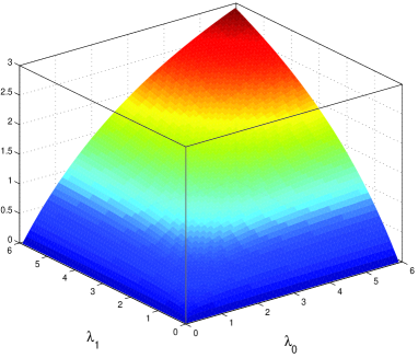
Figure 3: Steady-state translation rate $R(\lambda_{0},\lambda_{1})$ in the RFM with dimension $n=1$.

Recall that a function $f:\mathbb{R}^{k}_{+}\to\mathbb{R}$ is called positively homogeneous of degree $m$ if $f(cx)=c^{m}f(x)$ for all $c>0$ and all $x\in\mathbb{R}^{k}_{+}$. For example, the function $f(x_{1},x_{2}):=x_{1}x_{2}+x_{2}^{2}$ is positively homogeneous of degree $2$. The following result follows immediately from the fact that $R$ always appears in (7) only in terms of the form $R/\lambda_{i}$.

Fact 1

Consider the RFM with dimension $n$. The function $R=R(\lambda_{0},\dots,\lambda_{n})$ is positively homogeneous of degree one.

In other words,

$$R(c\lambda_{0},\dots,c\lambda_{n})=cR(\lambda_{0},\dots,\lambda_{n}),\quad\text{for all }c>0.$$ (10)

From a biophysical point of view this means that multiplying the initiation rate and all the elongation rates by the same factor $c>0$ increases of the steady-state production rate by a factor of $c$. This also means that the steady-state occupancy levels $e_{i}$, $i=1,2,\dots,n$, remain unchanged with respect to such a multiplication.

Example 2

Consider the RFM with dimension $n=2$. In this case, the feasible solution of (2) and (6) (i.e., the solution corresponding to a value $e\in C^{2}$ for all $\lambda_{0}$, $\lambda_{1}$, $\lambda_{2}>0$) is

$$R(\lambda_{0},\lambda_{1},\lambda_{2})=\frac{\lambda_{0}\lambda_{1}+\lambda_{0}\lambda_{2}+\lambda_{1}\lambda_{2}-\sqrt{(\lambda_{0}\lambda_{1}+\lambda_{0}\lambda_{2}+\lambda_{1}\lambda_{2})^{2}-4\lambda_{0}\lambda_{1}^{2}\lambda_{2}}}{2\lambda_{1}},$$ (11)

and clearly this implies that $R(c\lambda_{0},c\lambda_{1},c\lambda_{2})=cR(\lambda_{0},\lambda_{1},\lambda_{2})$.

Recall that a function $f:\mathbb{R}^{k}_{+}\to\mathbb{R}$ is called superadditive if $f(x+y)\geq f(x)+f(y)$ for all $x,y\in\mathbb{R}^{k}_{+}$. It is well-known that for a positively homogeneous function, concavity is equivalent to superadditivity (see, e.g., [4]). Combining this with Fact 1 and Theorem 1 yields the following result.

Corollary 1

Consider the RFM with dimension $n$. The function $R=R(\lambda_{0},\dots,\lambda_{n})$ is superadditive.

This means that

$$R(\lambda_{0}+\bar{\lambda}_{0},\dots,\lambda_{n}+\bar{\lambda}_{n})\geq R(\lambda_{0},\dots,\lambda_{n})+R(\bar{\lambda}_{0},\dots,\bar{\lambda}_{n}),$$

for all $\lambda_{0},\dots,\lambda_{n},\bar{\lambda}_{0},\dots,\bar{\lambda}_{n}>0$. From a biophysical point of view this means the following. Consider two RFMs, one with initiation rate $\lambda_{0}$ and transition rates $\lambda_{1}$, $\lambda_{2}$, $\dots$, $\lambda_{n}$, and the second with initiation rate $\bar{\lambda}_{0}$ and transition rates $\bar{\lambda}_{1},\bar{\lambda}_{2},\dots,\bar{\lambda}_{n}$. The sum of the production rates of these two RFMs is smaller or equal to the production rate of a single RFM with initiation rate $\lambda_{0}+\bar{\lambda}_{0}$ and transition rates $\lambda_{1}+\bar{\lambda}_{1},\lambda_{2}+\bar{\lambda}_{2},\dots,\lambda_{n}+\bar{\lambda}_{n}$. In other words, a single RFM with rates $\lambda_{i}+\bar{\lambda}_{i}$ is at least as efficient as the total of two separate RFMs, one with rates $\lambda_{i}$ and the second with rates $\bar{\lambda}_{i}$, for $i=0,1,\dots,n$.

3.2 Constrained Maximization of the Protein Translation Rate

Consider the problem of determining the parameter values $\lambda_{0},\dots,\lambda_{n}$ that maximize $R$ (or, equivalently, that minimize $-R$) in the RFM. Obviously, to make this problem meaningful we must constrain the possible parameter values. This leads to the following constrained optimization problem.

Problem 1

Given the parameters $w_{0},w_{1},\dots,w_{n},b>0$, minimize $-R=$ $-R(\lambda_{0},\dots,\lambda_{n})$, with respect to its parameters $\lambda_{0},\dots,\lambda_{n}$, subject to the constraints:

$$\sum_{i=0}^{n}w_{i}\lambda_{i} \leq b,$$ (12)

$$\lambda_{0},\dots,\lambda_{n} \geq 0.$$

In other words, given an affine constraint on the total rates, namely, the initiation rate $\lambda_{0}$ and the transition rates $\lambda_{1},\dots,\lambda_{n}$, maximize the protein translation rate. The constraint on $\lambda_{i}$, $i=0,1,\dots,n$, may be related to factors such as the abundance of intracellular ribosomes, initiation factors, intracellular tRNA molecules and elongation factors. The values $w_{i}$, $i=0,1,\dots,n$, can be used to provide different weighting to the different rates.

It is not difficult to show that the optimal solution $\lambda^{*}$ of Problem 1 always satisfies $\lambda^{*}\in\operatorname{{\mathrm{i}nt}}(R_{+}^{n+1})$. Theorem 1 implies that Problem 1 is a convex optimization problem [8]. It thus enjoys many desirable properties.

The next result shows that increasing any of the $\lambda_{i}$s increases the translation rate.

Proposition 1

Consider the RFM with dimension $n$. Then $\frac{\partial}{\partial\lambda_{i}}R>0$ for $i=0,1,\dots,n$.

In other words, increasing either the initiation rate or the elongation rate at any site improves the production rate.

Remark 1

Proposition 1 implies that the first constraint in (12) can be replaced by $\sum_{i=0}^{n}w_{i}\lambda_{i}=b$.

Example 3

Consider Problem 1 for the RFM with dimension $n=2$. In this case, $R$ is given by (11). Let $b=w_{0}=w_{1}=w_{2}=1$, i.e., the constraint is $\lambda_{0}+\lambda_{1}+\lambda_{2}=1$. Then $\lambda_{2}=1-\lambda_{0}-\lambda_{1}$, and substituting this in (11) yields

$$R= \frac{\lambda_{0}\lambda_{1}+(1-\lambda_{0}-\lambda_{1})(\lambda_{0}+\lambda_{1})}{2\lambda_{1}}$$

$$-\frac{\sqrt{(\lambda_{0}\lambda_{1}+(1-\lambda_{0}-\lambda_{1})(\lambda_{0}+\lambda_{1}))^{2}-4\lambda_{0}\lambda_{1}^{2}(1-\lambda_{0}-\lambda_{1})}}{2\lambda_{1}}.$$

Fig. 4 depicts this function. It may be seen that $R=0$ when either $\lambda_{0}=0$ or $\lambda_{1}=0$ (as a zero initiation or elongation rate means of course zero production rate), and also when $\lambda_{0}+\lambda_{1}=1$ (as then the elongation rate $\lambda_{2}=1-\lambda_{0}-\lambda_{1}=0$). The maximal value, $R^{*}=0.1294$, is obtained for $\lambda_{0}^{*}=0.3008$ and $\lambda_{1}^{*}=0.3984$, so $\lambda_{2}^{*}=1-\lambda_{0}^{*}-\lambda_{1}^{*}=0.3008$ (all numbers are to four digit accuracy). Note that (11) implies that $R(\lambda_{0},\lambda_{1},\lambda_{2})=R(\lambda_{2},\lambda_{1},\lambda_{0})$ for all $\lambda_{0},\lambda_{1},\lambda_{2}>0$, and since the constraint parameters satisfy $w_{0}=w_{2}$, we get $\lambda_{0}^{*}=\lambda_{2}^{*}$.

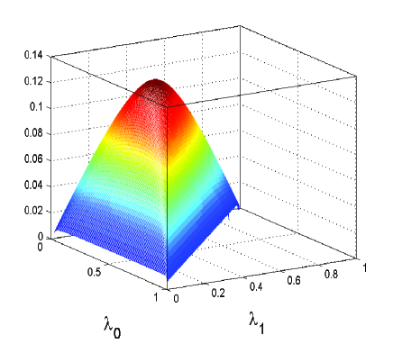
Figure 4: Steady-state translation rate $R$ in the RFM with dimension $n=2$ as a function of $\lambda_{0}$ and $\lambda_{1}$ under the constraint $\lambda_{2}=1-\lambda_{0}-\lambda_{1}$.

It is clear from (11) that in general an algebraic expression for $R$ in terms of $\lambda_{0},\dots,\lambda_{n}$ does not exist. It is possible however to give an algebraic expression for the maximal value $R^{*}$ as a function of just two optimal parameter values, namely, $\lambda_{0}^{*}$ and $\lambda_{1}^{*}$, and the parameters in the affine constraint.

Theorem 2

Consider Problem 1 for the RFM with dimension $n$. Then

$$R^{*}=\frac{(\lambda_{0}^{*})^{2}}{\lambda_{0}^{*}+\frac{w_{1}}{w_{0}}\lambda_{1}^{*}}.$$ (13)

In other words, the optimal translation rate $R^{*}$ can be computed given the optimal initiation rate and the first optimal elongation rate (and their corresponding weights in the affine constraint). This result holds regardless of the length of the transcript.

It is interesting to note that several biological studies showed that various signals encoded in the 5’UTR and the beginning of the ORF can predict the protein levels of endogenous genes with relatively high accuracy [33, 32, 70, 63, 47].

Example 4

Consider again Example 3. In this case $w_{1}/w_{0}=1$, $\lambda_{0}^{*}=0.3008$ and $\lambda_{1}^{*}=0.3984$, so (13) yields

$$R^{*}=\frac{0.3008^{2}}{0.3008+0.3984}=0.1294,$$

and this agrees with the result in Example 3.

3.2.1 Maximization with equal constraint weights

It is interesting to consider the specific case where all the weights $w_{i}$ in the constrained optimization problem are equal. Indeed, in this case the weights give equal preference to all the rates, so if the optimal solution satisfies $\lambda_{i}^{*}>\lambda_{j}^{*}$ for some $i,j$ then this may be interpreted as saying that, in the context of maximizing $R$, $\lambda_{i}$ is “more important” than $\lambda_{j}$.

Fig. 5 depicts the optimal values $\lambda_{i}$ for the case where $b=1$ and $w_{i}=1$ for all $i$. In other words, the constraint is $\sum_{i=0}^{n}\lambda_{i}=1$. Three cases are shown corresponding to $n=30$, $n=10$, and $n=4$. The optimal values were found numerically using a simple search algorithm that is guaranteed to converge for convex optimization problems.

It may be observed that the optimal transition rates are symmetric with respect to the index $i=n/2$. In general, the transition rate $\lambda_{n/2}^{*}$ is larger than all other rates and the optimal values decrease as we move towards any edge of the chain. The difference between $\lambda_{n/2}^{*}$ and $\lambda_{0}^{*}$ (or $\lambda_{n}^{*}$) is always visible, but the difference between $\lambda_{n/2}^{*}$ and $\lambda_{(n/2)\pm i}^{*}$, with $i$ small, becomes negligible as $n$ increases.

Intuitively, these results may be interpreted as follows. The importance of an elongation rate (or the corresponding site) depends on its “centrality”, or the mean distance of this site to other sites in the chain. Site $n/2$ is thus always the most “important” site in the chain. As $n$ increases, the sites near the middle site have almost the same mean distance to the other sites, and thus become almost as important.

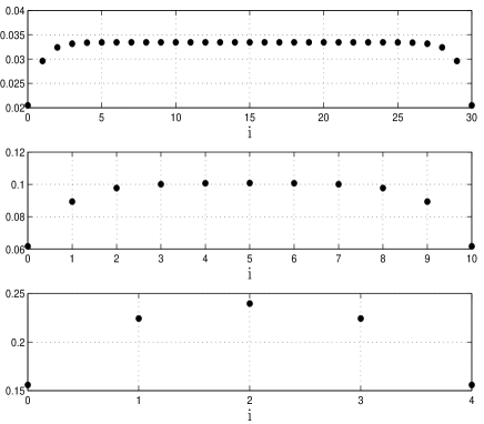
Figure 5: Optimal elongation rates $\lambda_{i}^{*}$ as a function of $i$ for the constraint $\sum_{i=0}^{n}\lambda_{i}=1$. Upper figure: $n=30$; Middle figure: $n=10$; Lower figure: $n=4$.

Fig. 6 depicts the optimal translation rate $R^{*}$ as a function of $n$ for two different constraints: $\sum_{i=0}^{n}\lambda_{i}=n$ and $\sum_{i=0}^{n}\lambda_{i}=n^{1.03}$. The first case corresponds to the scenario where the total available resources increases linearly with $n$ (i.e., $b=n$). It may be observed that in this case the optimal translation rate $R^{*}$ decreases monotonically with $n$. On the other hand, increasing the total available resources by a rate which is slightly larger than a linear rate (i.e., $b=n^{1.03}$) changes the behavior; $R^{*}$ in this case increases monotonically with $n$. This result suggests that in order to maintain the same optimal translation rate value as $n$ increases, the total allocated resources should increase at a rate that is slightly higher than a linear rate in $n$.

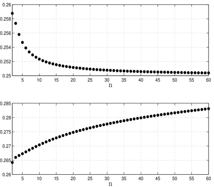
Figure 6: Optimal translation rate $R^{*}$ as a function of $n$ for the constraint $\sum_{i=0}^{n}\lambda_{i}=b$. Upper figure: $b=n$; Lower figure: $b=n^{1.03}$.

4 Discussion

The RFM is a deterministic mathematical model for translation-elongation. It can be derived via a mean-field approximation of a fundamental model from non-equilibrium statistical mechanics called TASEP. The RFM encapsulates both the simple exclusion and the total asymmetry properties of the stochastic TASEP model. The RFM is characterized by an order $n$, corresponding to the number of sites along the mRNA strand, a positive initiation rate $\lambda_{0}$ and a set of positive alongation rates $\lambda_{1},\dots,\lambda_{n}$.

In this paper, we show that the steady-state protein translation rate $R=R(\lambda_{0},\dots,\lambda_{n})$ in the RFM is a strictly concave function of its (positive) parameters. This implies that: (1) a local maximum of $R$ is the global maximum (and this maximum is unique); and (2) the problem of maximizing the steady-state protein translation rate under an affine constraint on the RFM parameters is a convex optimization problem. Such problems can be solved numerically using highly-efficient algorithms. The constraint here aims to capture the limited biosynthetic budget of the cell.

We now describe the possible implications of these results in various disciplines including biology, synthetic biology, molecular evolution, and functional genomics. As mentioned above, the functional dependence of the translation rate on various variables can also be examined experimentally. A recent paper [20] studied the effect of the intracellular translation factor abundance on protein synthesis. Experiments based on a tet07 construct were used to manipulate the production of the encoded translation factor to a sub-wild-type level, and measure the translation rate (or protein levels) for each level of the translation factor(s). An analysis of Fig. $1$ in [20] suggests that the mapping from levels of translation factors to the translation rate is indeed concave. Our results thus provide the first mathematical support for the observed concavity in these experiments.

In synthetic biology, re-engineering gene expression is frequently used to synthesize proteins for medical and agricultural goals [53, 43, 5, 21, 42]. For example, in genetically modified crops new genes are introduced to the genome of the host in order to improve its resistance to certain pests/diseases or for improving the nutrient profile of the crop [42]. Another example is the commercial production of human proteins in recombinant microorganisms for therapeutic use [53, 43, 5, 21]. This is sometimes based on the natural ability of certain bacteria to efficiently secrete properly folded human proteins (for example, insulin [21]). In this context, a fundamental problem is to maximize the translation rate of the heterologous gene (and thus the protein production rate) under the given constraints, e.g., the limited availability of intracellular components involved in translation. These constraints are needed also because very high initiation and elongation rates mean that the expression of the heterologous gene consumes too much resources of the translational machinery (e.g., ribosomes, tRNA molecules, etc), thus significantly deteriorating the fitness of the host. In addition, very high levels of protein abundance may eventually contribute to aggregation of proteins [45, 31], leading to a decrease in the yield of heterologous protein production. All these aspects are encapsulated in the convex optimization problem that is addressed here for the RFM. We believe that this mathematical problem may thus be used to provide verifiable predictions on how to efficiently manipulate the various biological factors.

There is a rich literature on using optimization theory, combined with evolutionary arguments, in biology (see, e.g., [54, 46, 2] and the references therein). This approach has been often criticized, but it has undoubtedly provided insight into the process of adaption under biological constraints, as well as helped to discriminate between alternative hypotheses for a suitable “fitness function” in various biological mechanisms. Furthermore, laboratory evolution experiments showed evolutionary adaptation of biological processes towards optimal operation levels. Examples include optimal metabolic fluxes in E. coli [26], and optimal protein expression levels from the lac operon [14]. We believe that the optimization problem posed here may lead to further progress in studying the evolution of the translation machinery.

The translation machinery is affected by mutations such as duplication/deletion of a tRNA gene or synonymous mutation affecting the codon bias usage. The concavity of the translation rate $R$ may suggest that the selection of mutations that increase fitness indeed converges towards the optimal parameter values, as explained by the simple “hill climbing” argument described above (see Fig. 7).

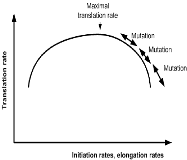
Figure 7: Evolutionary convergence to optimal translational state via mutations is similar to the simple “hill climbing” algorithm.

Recent studies have shown that in various organisms the ribosomal density at the $5^{\prime}$ and $3^{\prime}$ ends of the ORF is higher than in the middle of the ORF (see, for example, [28, 29, 11, 60]). In addition, the genomic ribosomal density is relatively constant in the middle of the ORF (usually more than $30$ codons away from the two ORF ends). The elongation rate $\lambda_{i}$ is negatively correlated with the ribosomal density (or the probability that a site is occupied) at site $i$. Indeed, if $\lambda_{i}$, that controls the elongation rate from site $i$, is small then there is a higher probability to see a ribosome in this site. Thus, these biological studies suggest that the elongation rates at the end of the chain are lower than in the middle of the chain, and that the rates near the middle are approximately equal. This agrees well with the optimal elongation rates derived based on our analysis in the case of equal weighting in the constraint (see Fig. 5).

Our results in the case of equal weights in the constraint also show that if the total biosynthetic budget $b(n)$ is a sub-linear or linear function of $n$ then $R^{*}$ decreases monotonically with $n$; however, when $b(n)$ grows faster than a linear function in $n$ then $R^{*}$ increases monotonically with $n$. The relation between expression levels and gene length has been studied experimentally. It has been shown that in some organisms, such as humans and S. cerevisiae [18, 12], expression levels tend to monotonically decrease with gene length (shorter genes have higher expression levels). However, in other organisms, such as plants [50], an opposite relation was reported (longer genes have higher expression levels). Our analysis may suggest that one should take into account not only the difference in gene length, but also the difference in the available resources of the translational machinery.

An interesting question for further research is whether the translation rate in other models of translation, including various versions of TASEP [41, 62, 60, 56, 10, 48], is also a concave function of its parameters.

Another possible research direction is the design and implementation of biological experiments based on the analytical results described above. Such experiments should combine: (1) methods for manipulating the translation machinery and/or the transcript of certain gene(s); and (2) online estimation of ribosomal density along the mRNA (e.g. using ribosome profiling [27]). The elongation rate of each codon can be estimated based on a method described in [13]. Manipulation of the translation machinery can include deletion of tRNA genes, and using the tet07 construct to down-regulate the initiation and elongation factors [20, 6]. Techniques for local manipulation of a transcript include generating libraries of a certain heterologous non-functional gene (e.g., a GFP protein). In each of the variants a few mutations (relatively to the wild-type) are introduced either in the 5’UTR (corresponding to $\lambda_{0}$) or the ORF (corresponding to $\lambda_{1},\lambda_{2},\dots$), and the protein levels and ribosomal densities are measured [33, 65]. The fact that the heterologous gene is non-functional to the host assures that the observed changes in translation efficiency are due to the introduced modifications.

As a specific example, one can measure the effect of modifying the elongation rates of different codons (corresponding to $\lambda_{1},\lambda_{2},..$) by introducing synonymous mutations in different parts of the ORF. We expect that a graph depicting the translation rate as a function of elongation rates will be concave (as in Fig. 4).

Finally, the effect of single mutations in different parts of the transcript on translation rate is a fundamental question related to various biomedical disciplines. Specifically, it is known that codon substitutions in different parts of the coding sequence affect elongation and initiation rates (i.e. the $\lambda_{i}$s) via various mechanisms (e.g. mRNA folding and adaptation to the tRNA pool [16, 22, 33, 62]). Our result is based on linking $R$ to the Perron root of a tridiagonal matrix that depends on the $\lambda_{i}$s. This can serve as a starting point for sensitivity analysis of $R$, i.e. analyzing the effect of small changes in the $\lambda_{i}$s on $R$. This topic is currently under study.

Appendix: Proofs

Proof of Theorem 1. The proof consists of the following steps:

1. Expressing the term on the right-hand side of (7) as a ratio between two polynomials $p(R)$ and $v(R)$.

2. Linking the numerator polynomial $p(R)$ to the determinant of a symmetric, non-negative tridiagonal matrix $A$ whose entries depend on the $\lambda_{i}$s.

3. Proving that $R^{-1/2}$ is the largest eigenvalue of the matrix $A$.

4. Using the properties of the largest eigenvalue of a symmetric, non-negative matrix to show that $R$ is a strictly concave function of its parameters.

Step 1: Define

$$g_{n+1}(z,\lambda_{0},\dots,\lambda_{n}):=1-\cfrac{z/\lambda_{0}}{1-\cfrac{z/\lambda_{1}}{1-\cfrac{z/\lambda_{2}}{\hphantom{aaaaaaa}\ddots\genfrac{}{}{0.0pt}{0}{}{1-\cfrac{z/\lambda_{n-1}}{1-z/\lambda_{n}}}}}}.$$ (14)

Then we can rewrite (7) as

$$g_{n+1}(R,\lambda_{0},\dots,\lambda_{n})=0.$$ (15)

By the theory of convergents of continued fractions [35] it follows that

$$g_{n+1}(z,\lambda_{0},\dots,\lambda_{n})=\frac{p_{n+1}(z,\lambda_{0},\dots,\lambda_{n})}{v_{n+1}(z,\lambda_{1},\dots,\lambda_{n})},$$ (16)

where $p_{n+1}$ and $v_{n+1}$ are defined recursively by

$$p_{-1}(z) =1,$$

$$p_{0}(z) =1,$$

$$p_{k}(z) =p_{k-1}(z)-z\lambda_{k-1}^{-1}p_{k-2}(z),\quad k\geq 1,$$ (17)

and

$$v_{-1}(z) =0,$$

$$v_{0}(z) =1,$$

$$v_{k}(z) =v_{k-1}(z)-z\lambda_{k-1}^{-1}v_{k-2}(z),\quad k\geq 1.$$ (18)

For example, for $n=2$ Eq. (14) yields

$$g_{3} =1-\cfrac{z/\lambda_{0}}{1-\cfrac{z/\lambda_{1}}{1-{z/\lambda_{2}}}}$$

$$=\frac{(\lambda_{0}^{-1}\lambda_{2}^{-1})z^{2}-(\lambda_{0}^{-1}+\lambda_{1}^{-1}+\lambda_{2}^{-1})z+1}{1-(\lambda_{1}^{-1}+\lambda_{2}^{-1})z},$$

whereas (Appendix: Proofs) and (Appendix: Proofs) yield

$$p_{3}=(\lambda_{0}^{-1}\lambda_{2}^{-1})z^{2}-(\lambda_{0}^{-1}+\lambda_{1}^{-1}+\lambda_{2}^{-1})z+1,$$

and

$$v_{3}=1-(\lambda_{1}^{-1}+\lambda_{2}^{-1})z.$$

Note that (Appendix: Proofs) and (Appendix: Proofs) imply that $p_{k}=p_{k}(z,\lambda_{0},\dots,\lambda_{k-1})$, $v_{k}=v_{k}(z,\lambda_{1},\dots,\lambda_{k-1})$, and

$$v_{k+1}(z,\lambda_{1},\dots,\lambda_{k})=p_{k}(z,\lambda_{0},\dots,\lambda_{k-1}).$$ (19)

Furthermore, (6) and (2) yield

$$e_{k}=\frac{p_{k}(R,\lambda_{0},\dots,\lambda_{k-1})}{p_{k-1}(R,\lambda_{0},\dots,\lambda_{k-2})},\quad k=1,\dots,n,$$ (20)

so

$$p_{k} =\frac{p_{k}}{p_{k-1}}\frac{p_{k-1}}{p_{k-2}}\dots\frac{p_{2}}{p_{1}}\frac{p_{1}}{p_{0}}$$

$$=e_{k}e_{k-1}\dots e_{1}.$$ (21)

Since $e_{i}\in(0,1)$ it follows that $p_{k}(R)\in(0,1)$ for all $k=1,2,\dots,n$.

From (15) and (16) it follows that

$$\frac{p_{n+1}(R,\lambda_{0},\dots,\lambda_{n})}{v_{n+1}(R,\lambda_{1},\dots,\lambda_{n})}=0.$$ (22)

Suppose for a moment that $v_{n+1}(R,\lambda_{1},\dots,\lambda_{n})=0$. Then (19) yields $p_{n}(R,\lambda_{0},\dots,\lambda_{n-1})=0$, and combining this with (20) yields $e_{n}=0$. This is a contradiction, as $e\in\operatorname{{\mathrm{i}nt}}(C^{n})$. We conclude that the denominator in (22) is not zero, so (22) is well-defined and so

$$p_{n+1}(R,\lambda_{0},\dots,\lambda_{n})=0.$$ (23)

Step 2: It is well-known that there is a close connection between continued fractions and tridiagonal matrices [64]. To relate the polynomial $p_{k}$ to a tridiagonal matrix, define the polynomials

$$q_{k}(s):=s^{k+1}p_{k}(s^{-2}),\quad k=-1,0,\dots,n+1,$$ (24)

where $s\in\mathbb{R}\setminus\{0\}$. Then (Appendix: Proofs) yields

$$q_{0}(s) =s,$$

$$q_{1}(s) =s^{2}-\lambda_{0}^{-1},$$

$$q_{k+1}(s) =sq_{k}(s)-\lambda_{k}^{-1}q_{k-1}(s),\quad k\geq 1.$$ (25)

Define a $(n+2)\times(n+2)$ Jacobi matrix $A=A(\lambda_{0},\dots,\lambda_{n})$ by

$$A:=\begin{bmatrix}0&\lambda_{0}^{-1/2}&0&0&\dots&0&0\\ \lambda_{0}^{-1/2}&0&\lambda_{1}^{-1/2}&0&\dots&0&0\\ 0&\lambda_{1}^{-1/2}&0&\lambda_{2}^{-1/2}&\dots&0&0\\ &&&\vdots\\ 0&0&0&\dots&\lambda_{n-1}^{-1/2}&0&\lambda_{n}^{-1/2}\\ 0&0&0&\dots&0&\lambda_{n}^{-1/2}&0\end{bmatrix}.$$ (26)

Let $I_{n+2}$ denote the $(n+2)\times(n+2)$ identity matrix. Then

$$sI_{n+2}-A=\begin{bmatrix}s&-\lambda_{0}^{-1/2}&0&0&\dots&0&0\\ -\lambda_{0}^{-1/2}&s&-\lambda_{1}^{-1/2}&0&\dots&0&0\\ 0&-\lambda_{1}^{-1/2}&s&-\lambda_{2}^{-1/2}&\dots&0&0\\ &&&\vdots\\ 0&0&0&\dots&-\lambda_{n-1}^{-1/2}&s&-\lambda_{n}^{-1/2}\\ 0&0&0&\dots&0&-\lambda_{n}^{-1/2}&s\end{bmatrix},$$

and it is straightforward to verify that the determinant of the $(i+1)\times(i+1)$ leading principal minor of $sI_{n+2}-A$ is $q_{i}(s)$. In particular, $q_{n+1}(s)=\det(sI_{n+2}-A)$. Combining (23) and (24) implies that $q_{n+1}(R^{-1/2})=0$, so $R^{-1/2}$ is an eigenvalue of the matrix $A$.

Step 3: Recall that the spectral radius of a square matrix is the maximum over the absolute values of its eigenvalue. The spectral radius of a non-negative matrix is an eigenvalue of the matrix called the Perron root [19]. The next result shows that $R^{-1/2}$ is the largest eigenvalue of the non-negative matrix $A$.

Proposition 2

The Perron root of the matrix $A$ is $R^{-1/2}$.

Proof of Proposition 2. It follows from known results on Jacobi matrices (see, e.g. [19, Chapter 0]) that all the eigenvalues of the matrix $A$ are real and distinct, and that if we order them as

$$\alpha_{1}<\alpha_{2}<\dots<\alpha_{n+2}$$

then the number of sign changes in the sequence

$$\{q_{n}(\alpha_{j}),\dots,q_{0}(\alpha_{j}),1\}$$

is $n+2-j$. Let $i$ be the index such that $\alpha_{i}=R^{-1/2}$. By (24), $q_{k}(\alpha_{i})=R^{-(k+1)/2}p_{k}(R)$, and (Appendix: Proofs) yields $q_{k}(\alpha_{i})>0$ for all $k=0,1,\dots,n$. Thus, the number of sign changes in the sequence $\{q_{n}(\alpha_{i}),\dots,q_{0}(\alpha_{i}),1\}$ is zero, so $i=n+2$, i.e. $\alpha_{n+2}=R^{-1/2}$. $\square$

Step 4: Given a vector $x=\begin{bmatrix}x_{0}&\dots&x_{n}\end{bmatrix}^{\prime}\in\operatorname{{\mathrm{i}nt}}(\mathbb{R}^{n+1}_{+})$, let $T(x)$ denote the $(n+2)\times(n+2)$ tridiagonal matrix whose main diagonal is zero, and sub- and super-diagonals are the vector $x$. Note that this matrix is non-negative and irreducible. Let $s_{i}=s_{i}(T(x))$, $i=1,\dots,n+2$, denote the eigenvalues of $T(x)$ ordered so that

$$s_{1}<s_{2}<\dots<s_{n+2}.$$

We already know that $s_{n+2}(T(x^{-1/2}))=R^{-1/2}(x)$. Note that the matrix $A$ in (26) can be written as $A=T(\lambda^{-1/2})$, where $\lambda^{-1/2}:=\begin{bmatrix}\lambda_{0}^{-1/2},\dots,\lambda_{n}^{-1/2}\end{bmatrix}^{\prime}$.

Pick $x,y\in\operatorname{{\mathrm{i}nt}}(\mathbb{R}^{n+1}_{+})$, with $x\not=y$, and $k\in(0,1)$. Let $u:=kx+(1-k)y$. Then

$$R(u)=s_{n+2}^{-2}(T(u^{-1/2})).$$ (27)

The function $f(w):=w^{-1/2}$ is strictly convex on $w\in(0,\infty)$, so

$$u^{-1/2}<kx^{-1/2}+(1-k)y^{-1/2},$$

where the inequality between the vectors should be interpreted component-wise. Since $T(u^{-1/2})$ is irreducible, this implies that [25, Chapter 8]

$$s_{n+2}\left(T(u^{-1/2})\right)<s_{n+2}\left(Q\right),$$

where $Q:=T(kx^{-1/2}+(1-k)y^{-1/2})$. Combining this with (27) yields

$$R(u)>s_{n+2}^{-2}(Q).$$ (28)

Since $Q$ is non-negative and symmetric, its induced $2$-norm is equal to its spectral radius $s_{n+2}(Q)$. Using the fact that a norm is always convex, it is straightforward to see that the norm-squared $s^{2}_{n+2}(Q)$ is also convex, so

$$s_{n+2}^{2}\left(Q\right) =s_{n+2}^{2}\left(kT(x^{-1/2})+(1-k)T(y^{-1/2})\right)$$

$$\leq ks_{n+2}^{2}\left(T(x^{-1/2})\right)+(1-k)s_{n+2}^{2}\left(T(y^{-1/2})\right).$$

Combining this with (28) yields

$$R(u) >\frac{1}{ks_{n+2}^{2}\left(T(x^{-1/2})\right)+(1-k)s_{n+2}^{2}\left(T(y^{-1/2})\right)}$$

$$\geq\min\left\{\frac{1}{s_{n+2}^{2}\left(T(x^{-1/2})\right)},\frac{1}{s_{n+2}^{2}\left(T(y^{-1/2})\right)}\right\}.$$

Now (27) implies that

$$R(kx+(1-k)y)>\min\{R(x),R(y)\},$$ (29)

i.e. $R$ is strictly quasi-concave on $\operatorname{{\mathrm{i}nt}}(\mathbb{R}^{n+1}_{+})$.

Pick $t\in(0,1)$, and let $\mu:=\frac{tR(x)}{tR(x)+(1-t)R(y)}$. Then $\mu\in(0,1)$, so (29) and the homogeneity of $R$ (see Fact 1 above) yield

$$R\left(\mu\frac{x}{R(x)}+(1-\mu)\frac{y}{R(y)}\right) >\min\left\{R\left(\frac{x}{R(x)}\right),R\left(\frac{y}{R(y)}\right)\right\}=1.$$

Thus,

$$R\left(\frac{tx+(1-t)y}{tR(x)+(1-t)R(y)}\right)>1.$$

Using the homogeneity of $R$ again gives

$$R\left(tx+(1-t)y\right)>{tR(x)+(1-t)R(y)},$$

and this completes the proof of Theorem 1. $\square$

Proof of Proposition 1. Let $v=\begin{bmatrix}v_{1}&\dots&v_{n+2}\end{bmatrix}^{\prime}\in\mathbb{R}^{n+2}_{+}$ denote a Perron eigenvector of the symmetric matrix $A$, i.e., an eigenvector corresponding to the Perron root $R^{-1/2}$. It follows from known results (see, e.g., [37]) that

$$\frac{\partial}{\partial\lambda_{i}}\left(R^{-1/2}\right)=\frac{v^{\prime}\left(\frac{\partial}{\partial\lambda_{i}}A\right)v}{v^{\prime}v},$$

and combining this with (26) yields

$$\frac{\partial}{\partial\lambda_{i}}R=\frac{2R^{3/2}}{\lambda_{i}^{3/2}v^{\prime}v}v_{i+1}v_{i+2}.$$ (30)

Since all the components of the Perron eigenvector are strictly positive [25], this implies that $\frac{\partial}{\partial\lambda_{i}}R>0$ for all $i=0,...,n$. $\square$

Proof of Theorem 2. The proof is based on formulating the Lagrangian function associated with Problem 1 and determining the optimal parameter values by equating its derivatives to zero (see, e.g., [8]). The Lagrangian is

$$L(\lambda_{0},\dots,\lambda_{n},\theta):=R(\lambda_{0},\dots,\lambda_{n})+\theta\left(b-\sum_{i=0}^{n}w_{i}\lambda_{i}\right),$$

where $\theta\in\mathbb{R}$ is the Lagrange multiplier. Differentiating this with respect to $\lambda_{i}$ and equating to zero yields

$$\theta w_{i}=\left(\frac{\partial}{\partial\lambda_{i}}R\right)|_{*},$$

where $|_{*}$ means that the equation holds once the optimal values $\lambda_{i}^{*}$ are substituted. This implies in particular that

$$\frac{w_{0}}{w_{1}}=\left(\frac{\frac{\partial}{\partial\lambda_{0}}R}{\frac{\partial}{\partial\lambda_{1}}R}\right)|_{*},$$

and combining this with (30) yields

$$\frac{w_{0}}{w_{1}}=\frac{(\lambda_{1}^{*})^{3/2}v_{1}^{*}}{(\lambda_{0}^{*})^{3/2}v_{3}^{*}},$$ (31)

where $v^{*}$ is the unique (up to scaling) Perron eigenvector of the non-negative and irreducible matrix $A^{*}:=A(\lambda_{0}^{*},\dots,\lambda_{n}^{*})$ [25, Ch. 8]. The equation $A^{*}v^{*}=(R^{*})^{-1/2}v^{*}$ yields

$$(\lambda_{0}^{*})^{-1/2}v_{2}^{*} =(R^{*})^{-1/2}v_{1}^{*},$$

$$(\lambda_{0}^{*})^{-1/2}v_{1}^{*}+(\lambda_{1}^{*})^{-1/2}v_{3}^{*} =(R^{*})^{-1/2}v_{2}^{*},$$

$$(\lambda_{1}^{*})^{-1/2}v_{2}^{*}+(\lambda_{2}^{*})^{-1/2}v_{4}^{*} =(R^{*})^{-1/2}v_{3}^{*},$$

$$\vdots$$

$$(\lambda_{n}^{*})^{-1/2}v_{n+1}^{*} =(R^{*})^{-1/2}v_{n+2}^{*}.$$ (32)

Thus

$$(\lambda_{1}^{*})^{-1/2}v_{3}^{*}=((R^{*})^{-1}(\lambda_{0}^{*})^{1/2}-(\lambda_{0}^{*})^{-1/2})v_{1}^{*},$$

and substituting this in (31) and simplifying yields (13). $\square$

References

- [1] B. Alberts, A. Johnson, J. Lewis, M. Raff, K. Roberts, and P. Walter, Molecular Biology of the Cell. New York: Garland Science, 2008.
- [2] U. Alon, “Biological networks: The tinkerer as an engineer,” Science, vol. 301, no. 5641, pp. 1866–1867, 2003.
- [3] D. Angeli, J. E. Ferrell, and E. D. Sontag, “Detection of multistability, bifurcations, and hysteresis in a large class of biological positive-feedback systems,” Proceedings of the National Academy of Sciences, vol. 101, pp. 1822–1827, 2004.
- [4] J. Baptiste, H. Urruty, and C. Lemarechal, Fundamentals of Convex Analysis. Springer, 2001.
- [5] C. Binnie, J. Cossar, and D. Stewart, “Heterologous biopharmaceutical protein expression in streptomyces,” Trends Biotechnol., vol. 15, no. 8, pp. 315–20, 1997.
- [6] Z. Bloom-Ackermann, S. Navon, H. Gingold, R. Towers, Y. Pilpel, and O. Dahan, “A comprehensive trna deletion library unravels the genetic architecture of the trna pool,” PLOS Genetics, vol. 10, no. 1, p. e1004084, 2014.
- [7] R. A. Blythe and M. R. Evans, “Nonequilibrium steady states of matrix-product form: a solver’s guide,” J. Phys. A: Math. Theor., vol. 40, no. 46, pp. R333–R441, 2007.
- [8] S. Boyd and L. Vandenberghe, Convex Optimization. Cambridge University Press, 2004.
- [9] C. Charneski and L. Hurst, “Positively charged residues are the major determinants of ribosomal velocity,” PLOS Biology, vol. 11, no. 3, p. e1001508, 2013.
- [10] D. Chu, N. Zabet, and T. von der Haar, “A novel and versatile computational tool to model translation,” Bioinformatics, vol. 28, no. 2, pp. 292–3, 2012.
- [11] A. Dana and T. Tuller, “Determinants of translation elongation speed and ribosomal profiling biases in mouse embryonic stem cells,” PLOS Computational Biology, vol. 8, no. 12, p. e1002755, 2012.
- [12] A. Dana and T. Tuller, “Efficient manipulations of synonymous mutations for controlling translation rate–an analytical approach,” J. Comput. Biol., vol. 19, pp. 200–231, 2012.
- [13] A. Dana and T. Tuller, “The effect of tRNA levels on decoding times of mRNA codons,” Nucleic Acids Res., 2014, to appear.
- [14] E. Dekel and U. Alon, “Optimality and evolutionary tuning of the expression level of a protein,” Nature, vol. 436, pp. 588–592, 2005.
- [15] C. Deneke, R. Lipowsky, and A. Valleriani, “Effect of ribosome shielding on mRNA stability,” Phys. Biol., vol. 10, no. 4, p. 046008, 2013.
- [16] M. dos Reis and L. Wernisch, “Estimating translational selection in eukaryotic genomes,” Molecular Biology and Evolution, vol. 26, no. 2, pp. 451–61, 2009.
- [17] S. Edri, E. Gazit, E. Cohen, and T. Tuller, “The RNA polymerase flow model of gene transcription,” IEEE Trans. Biomed. Circuits Syst., vol. 8, no. 1, pp. 54–64, 2014.
- [18] E. Eisenberg and E. Y. Levanon, “Human housekeeping genes are compact,” Trends Genet., vol. 19, no. 7, pp. 362–5, 2003.
- [19] S. M. Fallat and C. R. Johnson, Totally Nonnegative Matrices. Princeton University Press, 2011.
- [20] H. Firczuk, S. Kannambath, J. Pahle, A. Claydon, R. Beynon, J. Duncan, H. Westerhoff, P. Mendes, and J. McCarthy, “An in vivo control map for the eukaryotic mRNA translation machinery,” Mol Syst Biol., vol. 9, p. 635, 2013.
- [21] D. Goeddel, D. Kleid, F. Bolivar, H. Heyneker, D. Yansura, R. Crea, T. Hirose, A. Kraszewski, K. Itakura, and A. Riggs, “Expression in Escherichia coli of chemically synthesized genes for human insulin,” Proceedings of the National Academy of Sciences, vol. 76, no. 1, pp. 106–10, 1979.
- [22] W. Gu, T. Zhou, and C. O. Wilke, “A universal trend of reduced mRNA stability near the translation-initiation site in prokaryotes and eukaryotes,” PLOS Computational Biology, vol. 6, p. e1000664, 2010.
- [23] C. Gustafsson, S. Govindarajan, and J. Minshull, “Codon bias and heterologous protein expression,” Trends Biotechnol., vol. 22, pp. 346–353, 2004.
- [24] R. Heinrich and T. Rapoport, “Mathematical modelling of translation of mRNA in eucaryotes; steady state, time-dependent processes and application to reticulocytes,” J. Theoretical Biology, vol. 86, pp. 279–313, 1980.
- [25] R. A. Horn and C. R. Johnson, Matrix Analysis. Cambridge, 2013.
- [26] R. U. Ibarra, J. S. Edwards, and B. O. Palsson, “Escherichia coli K-12 undergoes adaptive evolution to achieve in silico predicted optimal growth,” Nature, vol. 420, pp. 186–189, 2002.
- [27] N. T. Ingolia, “Ribosome profiling: new views of translation, from single codons to genome scale,” Nat. Rev. Genet., vol. 15, no. 3, pp. 205–213, 2014.
- [28] N. T. Ingolia, S. Ghaemmaghami, J. R. Newman, and J. S. Weissman, “Genome-wide analysis in vivo of translation with nucleotide resolution using ribosome profiling,” Science, vol. 324, no. 5924, pp. 218–23, 2009.
- [29] N. T. Ingolia, L. Lareau, and J. Weissman, “Ribosome profiling of mouse embryonic stem cells reveals the complexity and dynamics of mammalian proteomes,” Cell, vol. 147, no. 4, pp. 789–802, 2011.
- [30] C. Kimchi-Sarfaty, T. Schiller, N. Hamasaki-Katagiri, M. Khan, C. Yanover, and Z. Sauna, “Building better drugs: developing and regulating engineered therapeutic proteins,” Trends Pharmacol. Sci., vol. 34, no. 10, pp. 534–548, 2013.
- [31] R. Kopito, “Aggresomes, inclusion bodies and protein aggregation,” Trends Cell Biol., vol. 10, no. 12, pp. 524–30, 2000.
- [32] M. Kozak, “Point mutations define a sequence flanking the AUG initiator codon that modulates translation by eukaryotic ribosomes,” Cell, vol. 44, no. 2, pp. 283–92, 1986.
- [33] G. Kudla, A. W. Murray, D. Tollervey, and J. B. Plotkin, “Coding-sequence determinants of gene expression in Escherichia coli,” Science, vol. 324, pp. 255–258, 2009.
- [34] P. D. Leenheer, D. Angeli, and E. D. Sontag, “Monotone chemical reaction networks,” J. Mathematical Chemistry, vol. 41, pp. 295–314, 2007.
- [35] L. Lorentzen and H. Waadeland, Continued Fractions: Convergence Theory, 2nd ed. Paris: Atlantis Press, 2008, vol. 1.
- [36] C. T. MacDonald, J. H. Gibbs, and A. C. Pipkin, “Kinetics of biopolymerization on nucleic acid templates,” Biopolymers, vol. 6, pp. 1–25, 1968.
- [37] J. R. Magnus, “On differentiating eigenvalues and eigenvectors,” Econometric Theory, vol. 1, pp. 179–191, 1985.
- [38] M. Margaliot, E. D. Sontag, and T. Tuller, “Entrainment to periodic initiation and transition rates in a computational model for gene translation,” PLoS ONE, vol. 9, no. 5, p. e96039, 2014.
- [39] M. Margaliot and T. Tuller, “On the steady-state distribution in the homogeneous ribosome flow model,” IEEE/ACM Trans. Computational Biology and Bioinformatics, vol. 9, pp. 1724–1736, 2012.
- [40] M. Margaliot and T. Tuller, “Stability analysis of the ribosome flow model,” IEEE/ACM Trans. Computational Biology and Bioinformatics, vol. 9, pp. 1545–1552, 2012.
- [41] M. Margaliot and T. Tuller, “Ribosome flow model with positive feedback,” J. Royal Society Interface, vol. 10, p. 20130267, 2013.
- [42] R. Mittler and E. Blumwald, “Genetic engineering for modern agriculture: challenges and perspectives,” Annu Rev Plant Biol., vol. 61, pp. 443–62, 2010.
- [43] T. Moks, L. Abrahmsen, E. Holmgren, M. Bilich, A. Olsson, G. Pohl, C. Sterky, H. Hultberg, and S. A. Josephson, “Expression of human insulin-like growth factor I in bacteria: use of optimized gene fusion vectors to facilitate protein purification,” Biochemistry, vol. 26, no. 17, pp. 5239–44, 1987.
- [44] E. Nurenberg and R. Tampe, “Tying up loose ends: ribosome recycling in eukaryotes and archaea,” Trends Biochem Sci., vol. 38, no. 2, pp. 64–74, 2013.
- [45] J. Park, K. Han, J. Lee, J. Song, K. Ahn, H. Seo, S. Sim, S. Kim, and J. Lee, “Solubility enhancement of aggregation-prone heterologous proteins by fusion expression using stress-responsive escherichia coli protein, RpoS,” BMC Biotechnol., vol. 8, p. 15, 2008.
- [46] G. A. Parker and J. Maynard Smith, “Optimality theory in evolutionary biology,” Nature, vol. 348, pp. 27–33, 1990.
- [47] J. Plotkin and G. Kudla, “Synonymous but not the same: the causes and consequences of codon bias,” Nat. Rev. Genet., vol. 12, pp. 32–42, 2011.
- [48] I. Potapov, J. Makela, O. Yli-Harja, and A. S. Ribeiro, “Effects of codon sequence on the dynamics of genetic networks,” J. Theoretical Biology, vol. 315, pp. 17–25, 2012.
- [49] J. Racle, F. Picard, L. Girbal, M. Cocaign-Bousquet, and V. Hatzimanikatis, “A genome-scale integration and analysis of Lactococcus lactis translation data,” PLOS Computational Biology, vol. 9, no. 10, p. e1003240, 2013.
- [50] X. Ren, O. Vorst, M. Fiers, W. Stiekema, and J. Nap, “In plants, highly expressed genes are the least compact,” Trends Genet., vol. 22, no. 10, pp. 528–32, 2006.
- [51] S. Reuveni, I. Meilijson, M. Kupiec, E. Ruppin, and T. Tuller, “Genome-scale analysis of translation elongation with a ribosome flow model,” PLOS Computational Biology, vol. 7, p. e1002127, 2011.
- [52] R. T. Rockafellar, “Lagrange multipliers and optimality,” SIAM Review, vol. 35, no. 2, pp. 183–238, 1993.
- [53] M. Romanos, C. Scorer, and J. Clare, “Foreign gene expression in yeast: a review,” Yeast, vol. 8, no. 6, pp. 423–88, 1992.
- [54] R. Rosen, Optimality Principles in Biology. London: Butterworths, 1967.
- [55] A. Schadschneider, D. Chowdhury, and K. Nishinari, Stochastic Transport in Complex Systems: From Molecules to Vehicles. Elsevier, 2011.
- [56] P. Shah, Y. Ding, M. Niemczyk, G. Kudla, and J. Plotkin, “Rate-limiting steps in yeast protein translation,” Cell, vol. 153, no. 7, pp. 1589–601, 2013.
- [57] L. B. Shaw, R. K. Zia, and K. H. Lee, “Totally asymmetric exclusion process with extended objects: a model for protein synthesis,” Phys. Rev. E Stat. Nonlin. Soft. Matter Phys., vol. 68, p. 021910, 2003.
- [58] H. L. Smith, Monotone Dynamical Systems: An Introduction to the Theory of Competitive and Cooperative Systems, ser. Mathematical Surveys and Monographs. Providence, RI: Amer. Math. Soc., 1995, vol. 41.
- [59] E. D. Sontag, “Monotone and near-monotone biochemical networks,” Systems and Synthetic Biology, vol. 1, pp. 59–87, 2007.
- [60] T. Tuller, A. Carmi, K. Vestsigian, S. Navon, Y. Dorfan, J. Zaborske, T. Pan, O. Dahan, I. Furman, and Y. Pilpel, “An evolutionarily conserved mechanism for controlling the efficiency of protein translation,” Cell, vol. 141, no. 2, pp. 344–54, 2010.
- [61] T. Tuller, M. Kupiec, and E. Ruppin, “Determinants of protein abundance and translation efficiency in s. cerevisiae.” PLOS Computational Biology, vol. 3, pp. 2510–2519, 2007.
- [62] T. Tuller, I. Veksler, N. Gazit, M. Kupiec, E. Ruppin, and M. Ziv, “Composite effects of gene determinants on the translation speed and density of ribosomes,” Genome Biol., vol. 12, no. 11, p. R110, 2011.
- [63] T. Tuller, Y. Y. Waldman, M. Kupiec, and E. Ruppin, “Translation efficiency is determined by both codon bias and folding energy,” Proceedings of the National Academy of Sciences, vol. 107, no. 8, pp. 3645–50, 2010.
- [64] H. S. Wall, Analytic Theory of Continued Fractions. Bronx, NY: Chelsea Publishing Company, 1973.
- [65] M. Welch, S. Govindarajan, J. Ness, A. Villalobos, A. Gurney, J. Minshull, and G. C., “Design parameters to control synthetic gene expression in Escherichia coli,” PLoS ONE, vol. 4, no. 9, p. e7002, 2009.
- [66] Y. Zarai, M. Margaliot, and T. Tuller, “Explicit expression for the steady-state translation rate in the infinite-dimensional homogeneous ribosome flow model,” IEEE/ACM Trans. Computational Biology and Bioinformatics, vol. 10, no. 5, pp. 1322–1328, 2013.
- [67] Y. Zarai, M. Margaliot, and T. Tuller, “Maximizing protein translation rate in the ribosome flow model: the homogeneous case,” IEEE/ACM Trans. Computational Biology and Bioinformatics, 2014, to appear. [Online]. Available: http://arxiv.org/abs/1407.0207
- [68] S. Zhang, E. Goldman, and G. Zubay, “Clustering of low usage codons and ribosome movement,” J. Theoretical Biology, vol. 170, pp. 339–54, 1994.
- [69] R. Zia, J. Dong, and B. Schmittmann, “Modeling translation in protein synthesis with TASEP: A tutorial and recent developments,” J. Statistical Physics, vol. 144, pp. 405–428, 2011.
- [70] H. Zur and T. Tuller, “New universal rules of eukaryotic translation initiation fidelity,” PLOS Computational Biology, vol. 9, no. 7, p. e1003136, 2013.