Specific heat anomaly in a supercooled liquid with amorphous boundary conditions (Includes SM)

Abstract

We study the specific heat of a model supercooled liquid confined in a spherical cavity with amorphous boundary conditions. We find the equilibrium specific heat has a cavity-size-dependent peak as a function of temperature. The cavity allows us to perform a finite-size scaling (FSS) analysis, which indicates the peak persists at a finite temperature in the thermodynamic limit. We attempt to collapse the data onto a FSS curve according to different theoretical scenarii, obtaining reasonable results in two cases: a “not-so-simple” liquid with nonstandard values of the exponents $\alpha$ and $\nu$, and random first-order theory (RFOT), with two different length scales.

In fragile glassformers, the relaxation time increases faster than the Arrhenius law as temperature is lowered Angell (1995). This implies that the effective barrier to relaxation grows on cooling, which leads to expect concomitant structural, and perhaps thermodynamic, changes. Though not universally accepted, the idea that a thermodynamic transition may underlie the dynamic glass transition is old and at the core of random first-order theory (RFOT) and other theoretical approaches Berthier and Biroli (2011). The question of the existence of a transition is open; in fact structural changes accompanying the slowdown have been found only recently Biroli et al. (2008); Widmer-Cooper et al. (2008); Lerner et al. (2009); Tanaka et al. (2010); Sausset and Levine (2011); Coslovich (2011); Charbonneau et al. (2012); Hocky et al. (2012); Kob et al. (2012), after more than a decade of study of dynamic correlations Ediger (2000); Sillescu (1999).

The most general tools for probing structural correlations are the “order-agnostic” methods —which include patch correlations Kurchan and Levine (2011); Sausset and Levine (2011), finite-size scaling (FSS) Fernández et al. (2006); Karmakar et al. (2009), point-to-set (PTS) Montanari and Semerjian (2006) and its related correlations— which do not need knowledge of the order parameter. Calculation of PTS correlations involves the study of confined systems, and in part for this reason a growing number of studies of liquids under various confined geometries have been reported, mainly cavities with amorphous boundary conditions (explained below) Bouchaud and Biroli (2004); Jack and Garrahan (2005); Cavagna et al. (2007); Biroli et al. (2008); Berthier and Kob (2012); Hocky et al. (2012), “cavities” with open directions Berthier and Kob (2012); Gradenigo et al. (2013) and systems with pinned particles Berthier and Kob (2012); Charbonneau et al. (2012); Karmakar and Parisi (2013). These investigations have focused mostly on density correlations, from which a correlation length can be extracted.

Here we report numerical results on the specific heat $C_{V}$ of a system confined under amorphous boundary conditions (ABCs), therefore combining the ABCs and standard FSS approaches . We find an anomalous peak as a function of temperature. The algorithm we use (swap Monte Carlo (MC) Grigera and Parisi (2001)) provides a complete sampling of configuration space at all the temperatures we report, so the peak is completely unrelated to the usual anomalies caused by the system falling out of equilibrium. We use FSS to study the changes of this thermodynamic anomaly as the cavity is enlarged, and our results indicate that it remains at a finite temperature in the thermodynamic limit. This is further evidence of the structural changes happening in supercooled liquids, and supports the existence of a thermodynamic transition.

We study the soft-sphere binary mixture of ref. Bernu et al. (1987) with size ratio 1.2 and unit density. To confine with ABCs, a spherical cavity of radius $R$ is created in an equilibrium configuration from a periodic boundary conditions (PBCs) system at temperature $T$, introducing a hard wall that conserves density and composition inside the cavity Cavagna et al. (2007); Biroli et al. (2008); Cavagna et al. (2010). Inside particles evolve with swap MC Grigera and Parisi (2001) at the same temperature, while outside particles are held fixed. The specific heat is computed through energy fluctuations, $C_{V}=\overline{[\langle E^{2}\rangle-\langle E\rangle^{2}]}/(MT^{2})$, where $E$ is the energy, $M$ the number of cavity (free) particles, and the overline means average over different realizations of the BCs. All results correspond to the (meta)equilibrium supercooled liquid. We used the energy time correlation function (checking for aging and finite-time effects) to estimate a correlation time and ensure that all relevant quantities were computed using runs lasting more than 100 relaxation times (including, self-consistently, the energy correlation). We used the bond orientation order parameter $Q_{6}$ Tanaka (2012) to exclude samples that showed signs of crystallization and could give a spurious contribution to the liquid $C_{V}$. Note that equilibration of small cavities is not problematic since with swap Monte Carlo smaller cavities are faster (not slower) than larger ones Cavagna et al. (2012). For detailed description of simulation and equilibration procedures and crystallization checks, see SM .

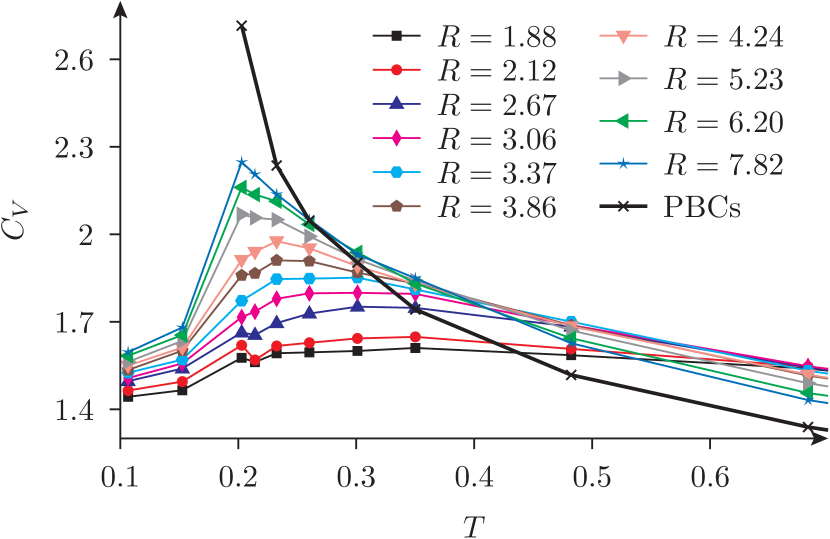
Figure 1: (color online) Specific heat vs. $T$ for amorphous boundary conditions (ABCs). Error bars omitted for clarity; the absolute error is bounded by 0.03. PBCs data are for a system of $N=8192$ particles, where $C_{V}$ can be measured down to $T\approx 0.2$ (see SM for details).

Fig. 1 shows the specific heat per mobile particle for ABCs for several cavity sizes (from 28 to 2000 mobile particles), displaying a peak. The peak is not due to the system going out of equilibrium, or to crystal formation. For classical liquids, $C_{V}$ is expected to be monotonically decreasing with temperature (as has been shown for a large number of liquid models Rosenfeld and Tarazona (1998); Ingebrigtsen et al. (2013) and follows from the phonon theory of liquids Bolmatov et al. (2012)): in this sense, the observed peak is an anomaly. A similar anomaly has been reported before Grigera and Parisi (2001); Yan et al. (2008), although in rather small systems and without a FSS analysis.

In the simplest scenario, the qualitative origin of this anomalous peak can be explained if we accept that the effect of the border penetrates into the cavity as far as a length-scale $\lambda(T)$, and that this penetration length increases for lower $T$ Cavagna et al. (2007). At very high $T$ the effect of the boundary is weak ($\lambda(T)$ is very small) and the $C_{V}$ of the liquid inside the cavity follows its bulk behavior (in our case well described at high $T$ by the Rosenfeld-Tarazona law $C_{V}\sim C_{V}^{\text{(b)}}=AT^{-2/5}$). For low $T$, on the other hand, $\lambda(T)$ will be large compared to the size $R$, so that the cavity will be almost frozen. The crossover from an increase to constant gives rise to the peak. Notice we have assumed no particular theory, nor any divergence of $\lambda(T)$ here, only that a very small cavity (relative to $\lambda$) is stuck. Hence, the mere presence of this peak does not allow us to discriminate among theoretical frameworks. We need to be more quantitative.

The penetration length $\lambda$ is conceptually different from the correlation length $\xi$ Cavagna et al. (2007); Zarinelli and Franz (2010); Gradenigo et al. (2013); Biroli and Cammarota (2014). The correlation length is a measure of the distance that two points must be separated form each other so that the local state is mutually independent (or in a cavity, how large must the cavity be so that the state at the center is independent from the state at the walls). The penetration length is only meaningful in the presence of domains, and is a measure of the width of the domain walls (in a cavity, how far from the wall a point must be to be independent from the state outside). $\xi$ can also be thought of as a measure of the size of the domains (or cooperatively rearranging regions), and $\lambda$ as a measure of the interface width, or the extent of the spatial fluctuations of the walls separating such domains or regions. The lengths can be coincide in simple cases (like the Ising model), but in principle they measure two different phenomena.

There are thus two sides in our finite-size story: a finite size is needed for the ABCs border to have an effect, but the converse is not true: with PBCs, for instance, we can have finite size but no border effects. Hence we must try to include, but separate, both effects: that of the ABCs border (related to $\lambda$) and that of the finite size (related to $\xi$). We believe a reasonable way to do this, at least near the peak, is to write

$$C_{V}(R,T)=R^{\alpha/\nu}\tilde{c}(y)[1-f(R/\lambda)].$$ (1)

The factor $R^{\alpha/\nu}\tilde{c}(y)$ is the border-free, FSS form of the specific heat, and it would be a safe bet in most finite-size systems with PBCs Newman and Barkema (1999). Through the scaling variable $y\equiv R^{1/\nu}(T-T_{c})/T_{c}$, the finite-size term contains all the information about the possible existence of a finite-temperature transition, $T_{c}$, and about the correlation length $\xi\sim(T-T_{c})^{-\nu}$; hence $\tilde{c}(y)$ is a function of $\xi/R$. The second factor on the r.h.s. is meant to take care of the border: for large $R/\lambda$ the border function $f\sim 0$ and the effect of the border is negligible (but not necessarily that of finite size). But we need to be more specific as regards $f(x)$ to test our scaling ansatz Eq. 1, so we make the simplest assumption: that the specific heat is zero exactly at the border and relaxes exponentially to the (finite-size) PBCs value. This results in Cavagna et al. (2007)

$$f(x)=3\left[x^{-1}-2x^{-2}+2x^{-3}(1-e^{-x})\right],$$ (2)

with $x=R/\lambda$.

This form of $f(x)$ is certainly an approximation; to understand its significance we must first make three remarks. First, Eq. 1 is qualitatively different from standard FSS only if $\lambda$ and $\xi$ are two different length scales, otherwise the effect of the border is a mere decoration of the scaling function and standard FSS remains unchanged. Second, in the critical region, $R\sim\xi$, which follows because the peak position is given by the position $y_{0}$ of the maximum of $\tilde{c}(y)$. This follows immediately in the usual FSS case; in the general case the analysis is slightly more complicated (see SM ), but it remains true that the peak position and its temperature shift are given by $R^{1/\nu}(T-T_{c})\simeq y_{0}$. Third, (at least in the scenarios we consider), $\lambda$ diverges at $T_{c}$, but not as fast as $\xi$.

When $R/\lambda\to\infty$, Eq. 2 gives correctly $f\to 0$. When $R/\lambda\to 0$, $f(x)$ tends unphysically to 1, but in the critical region $\lambda$ is large but $R\sim\xi$, so that $R/\lambda\ll 1$. This means the $R/\lambda\to 0$ limit of $f(R/\lambda)$ is irrelevant in the critical region. Very near $T_{c}$ though, (which is outside the critical region at finite size) our approximation will have the effect of making $\tilde{c}(y)$ divergent as $y\to 0$. Since this unwanted effect can be avoided at the expense of introducing unknown parameters, we have preferred to leave Eq. 2 as is. See SM for a discussion of this point and the possible cure.

Finally, note that in Eq. 1 there are two different mechanisms for the growth of the $C_{V}$ peak as $R$ increases. When there are no border effects, the $1-f(R/\lambda)$ factor is absent, and the growth of the peak is controlled by the $R^{\alpha/\nu}$ prefactor Newman and Barkema (1999). Hence, a nonzero $\alpha$ is normally required to explain a growing (eventually diverging for $R\to\infty$) peak. When there is a border, then the last factor also produces a (moderate) growth of the peak if $R$ grows faster than $\lambda$, so that $\alpha=0$ is compatible with a non-diverging growth of the specific heat for $T\to T_{c}$.

With this in mind, we now scale our finite-size data according to Eq. 1, namely we try to collapse the data by plotting, $C_{V}R^{-\alpha/\nu}[1-f(R/\lambda)]^{-1}$ vs. $R^{1/\nu}(T-T_{c})/T_{c}$. It is clearly useless to attempt to scale with all $T_{c}$, $\nu$, $\alpha$ and $\lambda(T)$ free, as there are too many parameters. We will rather try to compare different theoretical scenarios, thus fixing some of these parameters.

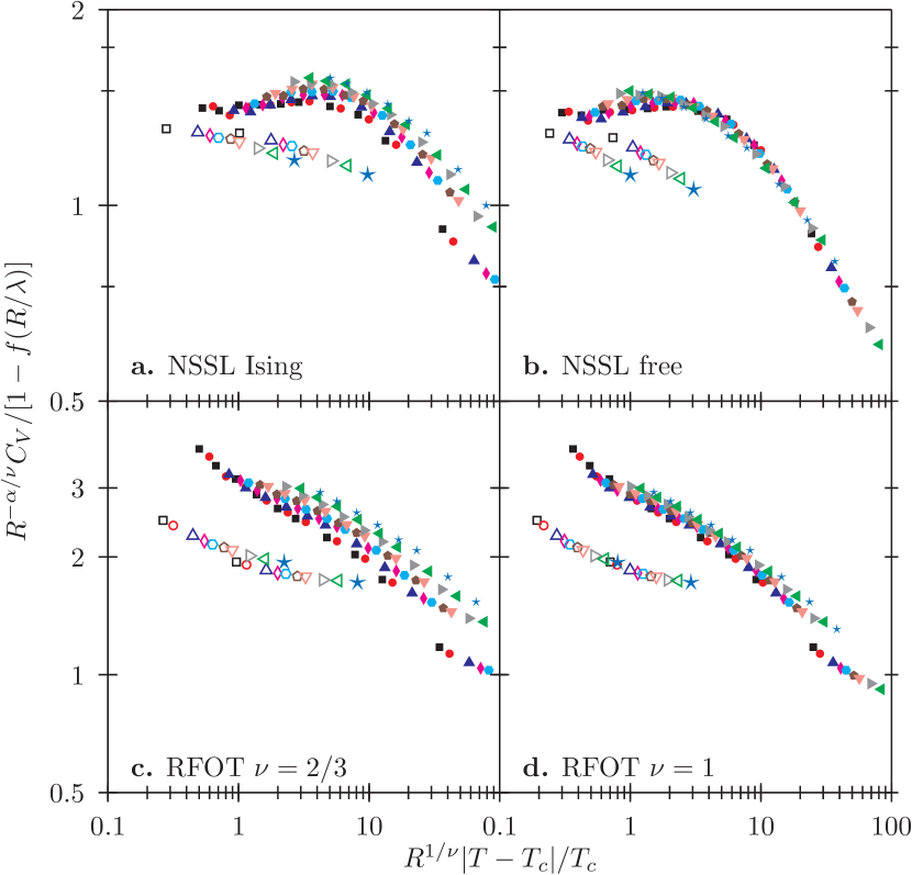
Figure 2: (color online) Attempts at scaling according to different theoretical scenarios. a: NSSL with Ising exponents ($f(x)\equiv 0$, $Tc=0.17$, $\alpha=0.11$, $\nu=0.63$). b: NSSL with free exponents ($f(x)\equiv 0$, $Tc=0.175$, $\alpha=0.2$, $\nu=1.0$). c: RFOT with $\nu=2/d$ ($\alpha\equiv 0$, $Tc=0.17$, $\nu=2/3$, $f(x)$ as in Eq. 2). d: RFOT with $\nu=1$ ($\alpha\equiv 0$, $Tc=0.17$, $f(x)$ as in Eq. 2). Colors and symbols indicate different radii (scheme as in Fig. 1), filled symbols are for $T>T_{c}$, open symbols for $T<T_{c}$.

Simplest liquid.

In the simplest possible physical scenario we have no transition ($T_{c}=0$) and only one length scale, $\lambda\sim\xi$ (i.e. $f\equiv 0$). In this case we are scaling the data as $C_{V}R^{-\alpha/\nu}$ vs $R^{1/\nu}T$. We then need $\alpha\neq 0$ to account for the growth of the peak. Moreover, it seems reasonable to assume that the standard RG scaling relation (Josephson scaling) $\nu d=2-\alpha$ Binney et al. (1992) holds in this simplest case. We are therefore left with just one parameter, $\alpha$. The result is quite bad and no reasonable collapse is obtained for any value of $\alpha$ (not shown).

Not-so-simple liquid (NSSL).

What really seems to resist the scaling of the data in the simplest case is the assumption $T_{c}=0$. We therefore relax this hypothesis, assuming that a standard phase transition exists at a finite temperature (standard meaning there is only one length scale, so that $\lambda\sim\xi$, and normal FSS ($f\equiv 0$) applies). One such case is that invoked by Tanaka et al. Tanaka et al. (2010), with Ising-like critical exponents (which thus satisfy the relation $\nu d=2-\alpha$). This proposal does not achieve a reasonable collapse, irrespective of the value of $T_{c}$ (Fig. 2a). Fernández et al. Fernández et al. (2006) have studied the specific heat of our same system under PBCs and seemed to find a divergence at temperature $T_{c}=0.195$, with $\alpha=0.9$. With these values, however, we fail to obtain a collapse (violating Josephson scaling does not help much either). If, however we leave all three parameters $\alpha$, $\nu$ and $T_{c}$ free, we get a reasonable collapse for the data above $T_{c}$ (Fig. 2b).

Mosaic liquid.

Now we assume that the penetration length, $\lambda$, and correlation length, $\xi$, grow differently. The increase of the peak for increasing $R$ implies that $\lambda\ll\xi$. This is the only case in which ABCs really have some nontrivial qualitative effect, because this is the only way in which we can achieve a growth of the peak with $\alpha=0$: in this case, the specific heat has a kink in the bulk limit, rather than a divergence. This is exactly what is supposed to happen in the random first-order theory (RFOT), as well as in some mean-field spin-glass models, in particular the $p$-spin Kirkpatrick and Thirumalai (1987); Crisanti and Sommers (1992); Coluzzi et al. (1999); Bouchaud and Biroli (2004). The RFOT transition is first order in the sense that it has a discontinuous order parameter, but second order in the Ehrenfest sense Crisanti and Sommers (1992); Coluzzi et al. (1999). Quite generally $\alpha=0$ in RFOT, as a consequence of the fact that the configurational entropy vanishes at $T_{c}$, giving a discontinuity of the derivative of the total entropy at the transition Crisanti and Sommers (1992); Coluzzi et al. (1999); Lubchenko and Wolynes (2007). There is theoretical Biroli and Cammarota (2014) as well as numerical Cavagna et al. (2007); Gradenigo et al. (2013) evidence that within the RFOT scenario indeed penetration and correlation length are different things and that $\lambda\ll\xi$.

In this scenario both $\xi$ and $\lambda$ diverge at $T_{c}$, but with different critical exponents. For $\lambda(T)$, the prediction is that $\lambda\sim\lvert T-T_{c}\rvert^{-1/2}$ in three dimensions Biroli and Cammarota (2014). The exponent ruling the $\xi$ divergence is $\nu=1/(d-\theta)$ Kirkpatrick et al. (1989), where $\theta$ is the stiffness exponent, for which different values have been predicted. Some approximations Kirkpatrick et al. (1989) give $\theta=d/2$, corresponding to $\nu=2/d$, while others Franz (2005); Gradenigo et al. (2013) give $\theta=d-1$, which yields instead $\nu=1$. In three dimensions, both predictions imply $\nu>1/2$ and thus $\xi\gg\lambda$ near $T_{c}$.

To perform the $\lambda\neq\xi$ scaling we need to plot $C_{V}R^{-\alpha/\nu}[1-f(\lambda/R)]^{-1}$ vs. $R^{1/\nu}(T-T_{c})/T_{c}$. We use Eq. 2 as an approximation for $f(x)$, but we need also $\lambda(T)$. For this we have taken the data of ref. Cavagna et al. (2007) and fitted them to a power law $a\lvert T-T_{c}\rvert^{1/2}$ Biroli and Cammarota (2014), leaving $a$ as fitting parameter but fixing $T_{c}$ self-consistently to the value that gives the best collapse of $C_{V}$. The resulting scalings are shown in Fig. 2 (panels c and d). Both have $\alpha=0$ in accordance to RFOT predictions, with $\lambda(T)$ for $T>T_{c}$ taken from the power law fit as explained above. $T_{c}$ is a free parameter, while $\nu$ is fixed to the values $2/3$ and $1$ according to the different predictions. The RFOT scaling with $\nu=2/3$ (Fig. 2c) does not give a good collapse of the data, while using $\nu=1$ does a rather good job (Fig. 2d) for $T>T_{c}$. For $T<T_{c}$ we do not have data to fit $\lambda(T)$, hence we have used the same power law with a prefactor $a^{\prime}$ chosen to give the best collapse. So the $T<T_{c}$ branch has a better-looking collapse but with two free parameters instead of one.

Though ABCs differ from more usual BCs such as PBCs in that they bring forward the existence of two lengthscales, the critical temperature and exponents are independent of the boundary conditions, since in the $R\to\infty$ limit all observables are independent of the boundary conditions unless control parameters are such that the system is below a thermodynamic transition Parisi (1998). It is not possible to perform the same analysis under PBCs in this system, because systems very small or below $T\approx 0.2$ crystallize before $C_{V}$ can be measured. The values we have been able to obtain are compatible with the NSSL scaling (Fig. 3c), but also with other values (see SM for more details). It is not possible to collapse the PBCs data using Eqs. 1 and 2, since $f(x)$ is constructed specifically for cavities (i.e. frozen boundaries). We do not delve into how the existence of two lengthscales as proposed by RFOT should manifest itself under PBCs; we merely point out that these data do not contradict a scaling with a nonzero critical temperature.

Finally, we have tried a different BC on a cavity, repeating the analysis with RBCs. RBCs are the same as ABCs except that the outer (fixed) particles are at random positions. Fig. 3 shows the result of applying the two most successful scalings to the RBCs data. This figure introduces no new parameters: RBCs data are scaled using the same $T_{c}$, $\lambda(T)$ and exponents adjusted for the ABCs case. Above $T_{c}$ both sets of data can be scaled with the same parameters, and, at least under RFOT, with the same scaling function. Below $T_{c}$ (open symbols), the scaling function seems to depend on the boundaries; we note in particular that the RBCs data can be scaled in the RFOT scenario without adjusting the prefactor of the $\lambda(T)$ power law.

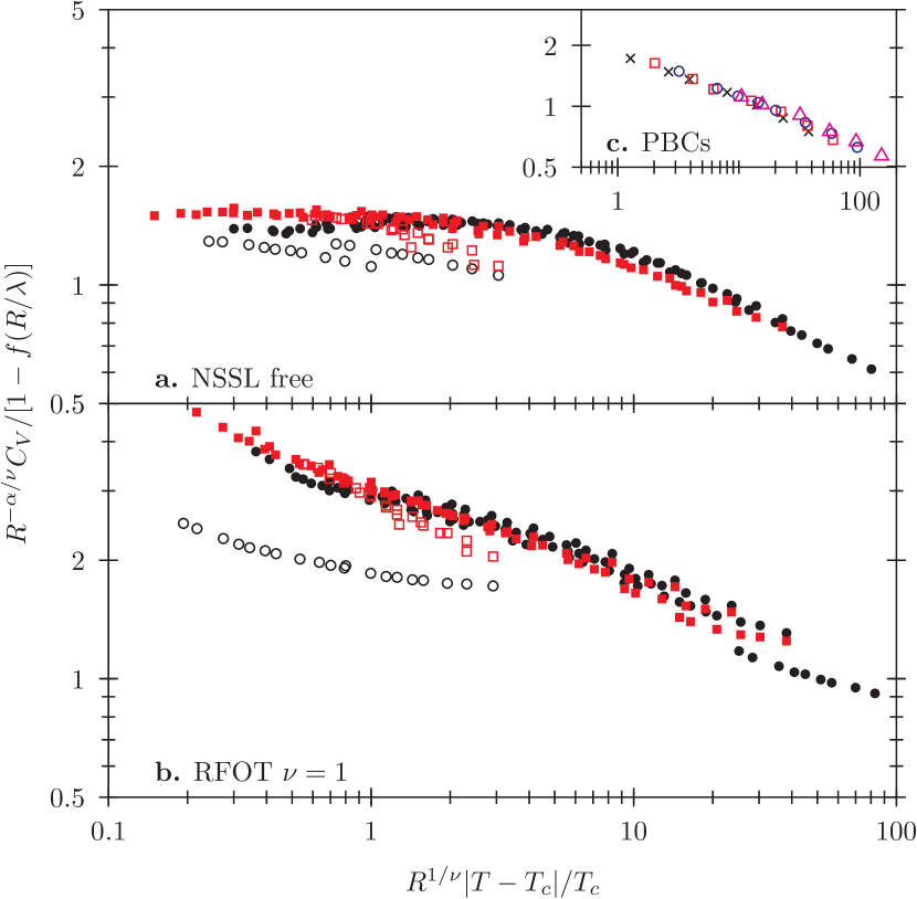
Figure 3: Scaling plots for $C_{V}$ data under random boundary conditions (RBCs) (red squares) and amorphous boundary conditions (ABCs) (black circles) according to the NSSL (panel a) and RFOT (panel b) scenarios. $T_{c}$, $\alpha$, $\nu$ and $\lambda(T)$ are the same for both sets of data and are those adjusted for ABCs and quoted in Fig. 2. The only difference is that in the RFOT case, we have set $a^{\prime}=a$ in the $\lambda(T)$ expression to scale RBCs data. Panel c: PBCs data for cubic systems of side $L=8$ (black crosses), 12.7 (red squares), 20.16 (blue circles), and 32 (purple triangles), scaled with the same exponents and $T_{c}$ of the NSSL case (panel a).

In summary, we have studied spherical cavities with amorphous and random BCs. Together with swap MC that can equilibrate small cavities, this has allowed us to do a FSS analysis of the specific heat, which is impossible under PBCs due to crystallization. We have found a peak in $C_{V}$, which can be scaled under two different scenarios, NSSL and RFOT. The first implies a divergence of $C_{V}$ in the thermodynamic limit, while the second predicts a discontinuity. Both are of comparable quality, but NSSL has three free parameters, compared to one (two below $T_{c}$) for RFOT. Within RFOT, only $\nu=1$ gives a reasonable collapse, suggesting a stiffness exponent $\theta=d-1$.

We finally emphasize that in all cases our collapse attempts yield a finite $T_{c},$ of around 0.17. This means that the peak survives the thermodynamic limit. Since in this limit observables must be independent of the boundary conditions (unless there is phase coexistence ), this result implies the existence of an anomaly or phase transition in the $R\to\infty$ limit, independently of the particular BCs we have employed. Investigation of more realistic and better glassforming liquids is needed. This will be a challenge, as swap MC is unsuitable for most systems. Nevertheless, these results seem a strong support for thermodynamic theories of the glass transition.

Supplemental Material

Appendix A Simulation details

We have used the soft-sphere binary mixture of ref. Bernu et al. (1987) at unit density, with size ratio 1.2, and a smooth cut-off (details as in ref. Biroli et al. (2008)). The numerical work involves two stages: preparation of the cavity and simulation of the cavity with the frozen environment.

For the amorphous boundary conditions (ABCs) runs, the frozen border must be taken from an equilibrated configuration at the same temperature at which the cavity will be run. To obtain these configurations we ran systems of $N=8192$ soft spheres with PBCs using swap Monte Carlo Grigera and Parisi (2001) for temperatures $T=1$, $0.683$, $0.482$, $0.350$, $0.301$, $0.260$, $0.232$, $0.214$, $0.203$, $0.153$, and $0.107$. At each temperature, 8 to 16 samples were simulated until equilibration. For RBCs, we simply generated 16 random configurations. Additionally PBCs systems of size $N=512$, $N=2048$, and $N=32768$ were equilibrated for high ($T\geq 0.203$) temperatures, which were later used to obtain the PBCs $C_{V}$ data.

From the equilibrated or random configurations, cavities were generated by adding to the periodic system a hard wall of spherical shape such that density and composition within the wall are identical to those of the PBCs system. Then the cavity runs were carried out, using swap Monte Carlo as before but keeping the positions of the particles outside the wall unchanged. We used walls of radii $R=1.88$, $2.12$, $2.67$, $3.06$, $3.37$, $3.86$, $4.24$, $5.23$, $6.20$, and $7.26$, corresponding to cavities containing from $M=28$ to 2000 particles. The cavities were then run, in the case of ABCs at the temperatures listed above, and in the case of RBCs at those temperatures plus $T=0.183$, $0.173$, $0.135$, and $0.120$.

The cavities were equilibrated and $C_{V}$ was measured from the energy fluctuations:

$$C_{V}=\overline{[\langle E^{2}\rangle-\langle E\rangle^{2}]}/(MT^{2}),$$ (3)

where $E$ is the energy and $M$ is the number of mobile (cavity) particles, units are such that Boltzmann’s constant is unity, and the overline means average over different realizations of the boundary (fixed particles). In ABCs we cannot compute $C_{V}$ as $d\overline{E}/dT$, because the derivative and the average do not commute (in fact this expression gives just the bulk $C_{V}$ Cavagna et al. (2010); Zarinelli and Franz (2010); Krakoviack (2010)).

We have used 8 to 40 samples per radius and temperature, with sample error ${\Delta Cv\over Cv}\lesssim 0.025$ for ABCs and ${\Delta Cv\over Cv}\lesssim 0.1$ for RBCs and (high temperature) PBCs.

Simulations were performed in a 192 core Xeon E5506 2.13Ghz cluster, devoted for this project for about one year.

Appendix B Equilibration

For all our runs, we computed the (connected) energy autocorrelation function,

$$C(t)=\left\langle\left[E(0)-\langle E\rangle\right]\left[E(t)-\langle E\rangle\right]\right\rangle.$$ (4)

We estimated the relaxation time as time $\tau$ such that $C(\tau)=C(0)/10$, and we let the simulations run for at least $25\tau$ before starting the data collection stage, which lasted at least $100\tau$. This procedure was performed self-consistently, in the sense that the runs used to estimate $\tau$ were themselves at least $100\tau$ long. To compute $C_{V}$ we used runs longer than $500\tau$; for ABCs cavities, the runs were more than $1000\tau$ long.

To ensure that $\tau$ was not underestimated due to the finite length of the time series, we required that $\lvert C(t)\rvert<0.03$ for at least 80% of the time values. We show four representative autocorrelation functions in Fig. 4, and the estimated values of $\tau$ for all our ABCs cavities in Fig. 5. One should keep in mind that we are using swap Monte Carlo. This is especially important for the cavity runs, because with standard Monte Carlo the relaxation time increases quickly as cavity size is reduced Hocky et al. (2012), while relaxation time decreases for smaller cavities when using swap moves, as was found in ref. Cavagna et al., 2012 looking at overlap autocorrelation and is clear from the present data (Figs. 4 and 5). Also, the correlation times display a peak qualitatively similar to that of $C_{V}$. The significance of this, however, is not immediately obvious, since we are employing an unrealistic dynamics. A further analysis of these data will be published elsewhere.

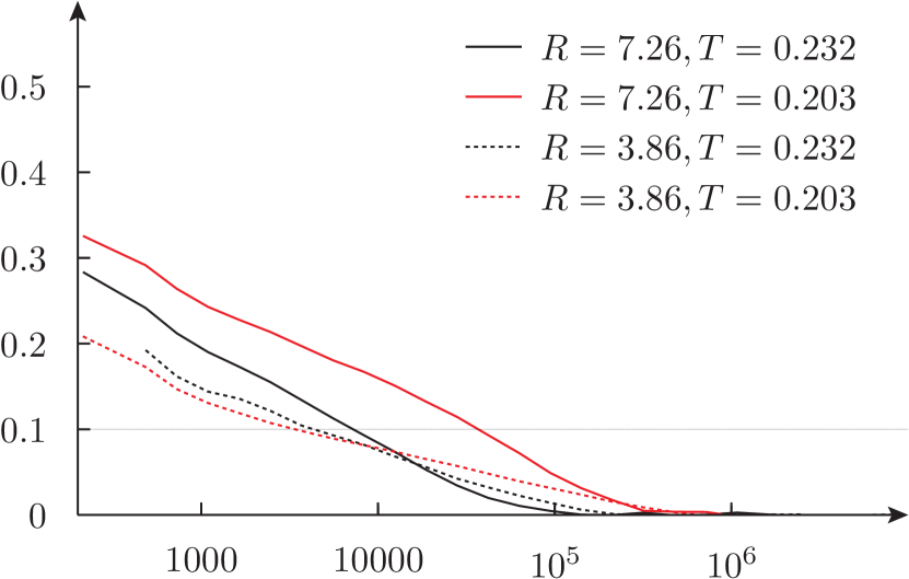
Figure 4: Representative energy autocorrelation function vs. time for two ABCs cavities at two temperatures

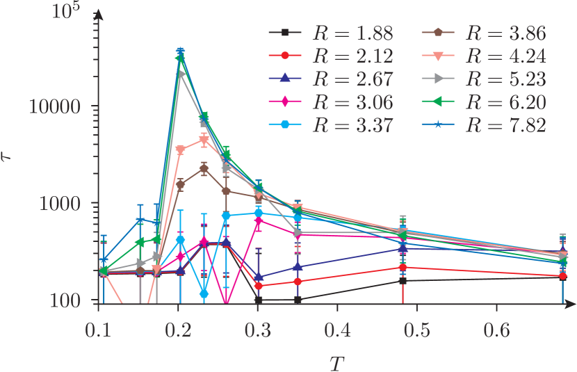
Figure 5: Correlation times for ABCs, computed as the time when the correlation decays to 10% of its initial value. These data include only noncrystallised samples.

Appendix C Crystallization

For a stable thermodynamic phase, the above conditions can in principle be fulfilled for each and every sample, given long enough simulation time. However, we are simulating a metastable phase (the supercooled liquid) in finite dimension, which thus has a finite lifetime. Accordingly, some of the samples have to be discarded because signs of crystallization appear before the requirements we imposed can be fulfilled.

Supercritical crystal nuclei appeared before equilibration or before measurement of $C_{V}$ could be completed in a temperature-dependent fraction of the samples. This was manifested in jumps or drifts of the energy and/or negative correlation values at long times. Once a supercritical nucleus appears, the ensuing coarsening process may last for a long time. Thus rather than attempting to bring all samples to equilibrium, we discarded samples that failed to equilibrate when most (more than 75%) of the samples at the same temperature had equilibrated according to the above requirements.

Of course, it can also happen that a crystal structure develops that is sufficiently stable to pass the above equilibration check, so for all samples that passed our equilibration criteria we computed the bond orientation order parameter Tanaka (2012),

$$Q_{l}=\sqrt{{4\pi\over 2l+1}\sum_{m=-l}^{m=l}|\langle Q_{lm}(\mathbf{r}_{ij})\rangle|^{2}},$$ (5)

where $\mathbf{r}_{ij}=\mathbf{r}_{j}-\mathbf{r}_{i}$, $\langle\ldots\rangle$ means average over neighbouring particles (those whose distance is less that the first minimum in the pair correlation function), and $Q_{lm}(\mathbf{r}_{ij})=Y_{lm}(\theta(\mathbf{r}_{ij}),\phi(\mathbf{r}_{ij}))$, with $Y_{lm}$ the spherical harmonics. We have considered $Q_{6}$, which takes the value of $0.3535$ for SC crystals, $0.5745$ for FCC, and intermediate values for other relevant crystal structures (such as BC and HCP) liquid-thermodynamics:steinhardt83, while for a random configuration, $Q_{6}=Q_{6}^{\text{(ran)}}=1/\sqrt{N_{\text{bonds}}}\simeq 1/\sqrt{6N}$ structure:errington03. In addition to the equilibration requirements, we have rejected all samples with $\langle Q_{6}\rangle>5Q_{6}^{\text{(ran)}}$. In the worst cases (for PBCs at $T=0.203$, and RBCs for the two largest radii at $T=0.120$ and $T=0.107$), half of the samples failed one of the tests and were excluded from the study. For $T>0.2325$ all the samples passed the tests, in other cases about 25% of the samples had to be discarded.

Appendix D Finite-size and border effects

When using PBCs, finite-size effects are taken into account by introducing a scaling function $\tilde{c}(y)$, which depends on the ratio of size to correlation length, $R/\xi$, and is unspecified except for its limiting behavior. The scaling variable is then $y=(R/\xi)^{1/\nu}=R^{1/\nu}\lvert T-T_{c}\rvert/T_{c}$, and the scaling prediction can be tested by plotting the data against $y$. In our cavity case, however, we have two lengthscales, $\xi$ and $\lambda$, so we expect

$$C_{V}(R,T)=\tilde{g}(R/\xi(T),R/\lambda(T)).$$ (6)

Having two scaling variables means that we have not reduced the number of variables, and thus cannot easily check our scaling by plotting against the scaling variables. We have thus to specify explicitly the dependence on one of them so that we can do our scaling analysis. In the main text we have accordingly proposed

$$C_{V}(R,T)=R^{\alpha/\nu}\tilde{c}(y)[1-f(R/\lambda(T))].$$ (7)

This is clearly an approximation, motivated by a microscopic model. It suffers of several shortcomings, but we have stuck to it because it introduces the least number of unknown parameters. We discuss below the microscopic model that leads to Eq. 7, its limitations, and why these do not matter in the critical region, which has finally led us to use it despite those limitations.

The function $f(R/\lambda)$.

Consider the specific heat (per unit volume) of a very small volume at distance $r$ from the center of a cavity of radius $R$, $c(r,R)$ such that the penetration length is large. Since the outside particles are frozen, precisely at the border $c(R,R)$ will be very small or zero. At a microscopic distance $\sigma$ away from the border, configurational rearrengements will still be blocked by the surface field produced by the outside particles, but we expect vibrations to be possible, leading to $c(R-\sigma,R)=C_{0}\approx 3/2$. Further away, we assume an exponential decay towards the PBCs (border-free) value $C_{P}$. Hence we propose

$$c(r,R)=\begin{cases}C_{P}+\Delta C_{V}e^{-(R-\sigma-r)/\lambda},&r<R-\sigma,\\ C_{0}(R-r)/\sigma,&R-\sigma<r\leq R\end{cases}$$ (8)

where $\Delta C_{V}=C_{0}-C_{P}$.

The specific heat of the cavity is then obtained by integrating over the whole sphere, $C_{V}(R)=(3/R^{3})\int_{0}^{R}\!\!dr\,r^{2}c(r,R)$, resulting in

$$\begin{split}C_{V}(R,T)={}&(1-\sigma/R)^{3}C_{P}\left\{1-f\left[(R-\sigma)/\lambda\right]\right\}+\\ &(1-\sigma/R)^{3}C_{0}f\left[(R-\sigma)/\lambda\right]+h(\sigma/R),\end{split}$$ (9)

where $f(x)$ is given by Eq. 2 of the main text and the last term is a microscopic contribution

$$h(x)=3C_{0}x\left(\frac{1}{2}-\frac{2x}{3}+\frac{x^{2}}{4}\right).$$ (10)

Finite-size, non-border effects are then taken into account by writing $C_{P}=R^{\alpha/\nu}\tilde{c}(y)$. When $\sigma=0$ and $C_{0}=0$, Eq. 9 reduces to Eq. 7.

For $R\gg\sigma$ and $\lambda\to\infty$, Eq. 9 gives $C_{V}\to C_{0}$. Thus it seems reasonable to keep $C_{0}\neq 0$, unlike what we have done. One can indeed do so, but it turns out that $C_{0}$ and $\sigma$ cannot be arbitrary: for a given $\sigma$, only one value of $C_{0}$ will make the curves collapse. In particular, for $\sigma=0$, this value is $C_{0}=0$. This relationship can be better understood through the following considerations, which show that the value $C_{0}$ actually never plays the role of an observable quantity.

The critical region.

The critical region is defined by a finite value of $y$ ($y_{0}$ say), so that in this region $R\sim\xi$. This is where the transition should take place, because the correlation length is of the order of the system size. When there are no border effects, the peak (i.e. the finite-size transition) is readily found to occur at $T_{p}=T_{c}+y_{0}T_{c}/(R^{1/\nu})$, where $y_{0}$ is the position of the maximum of $\tilde{c}(y)$. Including the border contributions in Eq. 9, the condition for $C_{V}$ to have a maximum (at fixed $R$) is

$$\tilde{c}^{\prime}(y)=\frac{c(y)-R^{-\alpha/\nu}C_{0}}{1-f(x)}\frac{f^{\prime}(x)R^{-1/\nu}(R-\sigma)}{\lambda^{2}}\frac{\partial\lambda}{\partial T},$$ (11)

with $x=(R-\sigma)/\lambda$. Since $f^{\prime}(x)\sim x^{-2}$, $\partial\lambda/\partial T\sim\lambda^{3}$, and $\lambda\sim\lvert T-T_{c}\rvert^{1/2}\sim\xi^{1/2\nu}$, the r.h.s. is of order $R^{-1/\nu}\lambda^{3}/R\sim R^{1/2\nu-1}$, so that self-consistently near the peak at large $R$ the maximum is given by a finite value of $y$ near $y_{0}$, and $R\sim\xi$.

The limit $R/\lambda\to 0$.

In RFOT the length $\lambda$ diverges as $T\to T_{c}$, as does $\xi$, but with a smaller exponent, so that $\xi\gg\lambda$. It follows that the limiting value $f_{0}\equiv\lim_{x\to 0}f(x)$ is irrelevant in the critical region, because there $R/\lambda\sim\xi/\lambda\gg 1$.

The value of $f_{0}$ plays a role at $T_{c}$ (i.e. outside the critical region for finite samples), as can be seen inverting Eq. 9:

$$\tilde{c}(y)=R^{-\alpha/\nu}\frac{\left[C_{V}(R,T)-h(\frac{\sigma}{R})\right](1-\frac{\sigma}{R})^{-3}-C_{0}f[\frac{R-\sigma}{\lambda}]}{1-f[\frac{R-\sigma}{\lambda}]}.$$ (12)

Since $\lambda\to\infty$ at $T_{c}$ and $f_{0}=1$ for our $f(x)$, $\tilde{c}(y)$ will develop a divergence for $y\to 0$ unless a delicate cancellation occurs in the numerator. In particular, when $C_{0}=\sigma=0$, there is no cancellation and $\tilde{c}(y\to 0)$ diverges. This is inconsistent with the expectation that $\tilde{c}(y)$ is the PBCs scaling function, which is defined to be finite at $y=0$. The origin of this problem is explained next.

Diverging $\lambda$ and finite cavities.

The basic idea of FSS is that $\xi$ in a finite system is never infinite, but is cut-off by the system size $R$. This is how the properties of the scaling function are inferred Newman and Barkema (1999). Clearly, the same applies to $\lambda$. However, our simple model for the border effects does not incorporate this: that is the reason for the divergence of the scaling function at small $y$. The function $\tilde{c}(y)$ diverges to compensate for the unphysical feature of an infinite $\lambda$ at $T_{c}$ and finite $R$. One way to cure this would be to replace $\lambda$ by an effective length $l(R/\lambda)$, given by

$$l(R/\lambda)=R\tilde{l}(R/\lambda),\qquad\tilde{l}(x)=\begin{cases}\text{const},&x\to 0,\\ x^{-1},&x\to\infty,\end{cases}$$ (13)

so that $l$ remains finite for $T\sim T_{c}$ when $R$ is finite. This can be done (see Fig. 6), but the cost is to introduce many additional unknowns.

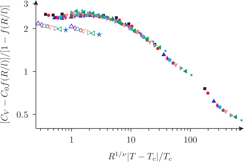
Figure 6: Scaling of ABCs data using Eqs. 9 and $l(x)=1/(D_{0}+x)$. Parameters are $\nu=1$, $\alpha=0$, $Tc=0.175$, $C_{0}=0$, $\sigma=0.2$, $D_{0}=20$.

Summary.

The value of the specific heat at the border of the cavity set by a particular microscopic model is irrelevant in the critical region where $R\sim\xi\gg\lambda$. Our simple Eqs. 1 and 2 of the main text suffer from a more drastic problem: they unphysically allow for $\lambda$ to become actually infinite at $T=T_{c}$ and finite $R$. Because of this, the microscopic details artificially show up near $T_{c}$, with the result that the estimated scaling function $\tilde{c}(y)$ has to compensate for this shortcoming of our treatment of border effects, differing (even possibly diverging) from the PBCs scaling function at small $y$. While this problem can be cured by introducing an effective $l(R/\lambda)$ as shown above, this involves additional unknowns. We have hence decided to keep unknown constants to a minimum, at the expense of not correctly estimating $\tilde{c}(y)$ for small $y$. We repeat, though, that these issues do not affect the critical region.

Appendix E Periodic boundary conditions

Since our FSS analysis points to a result (a finite $T_{c}$) that holds in the thermodynamic limit independently of the boundary conditions, it is natural to ask whether this result could be obtained using the more usual PBCs. We have shown in the main text (Fig. 3) that PBCs data are compatible with the scaling that yields a finite $T_{c}$. Here we explain in more detail why PBCs data are however not enough to establish such scaling.

Basically, with PBCs one can obtain much less datapoints of $C_{V}$ due to crystallization. While the spherical geometry makes crystallisation very rare for cavities (and rarer for the smaller ones), in the periodic geometry crystallization occurs too quickly to obtain meaningful data for $N\lesssim 500$ particles and temperatures below $\approx 0.26$. In larger systems the problem is less severe, but lower temperatures are still problematic. While we have been able to thermalize 8192 particles down to $T=0.107$ as stated above, this does not mean that $C_{V}$ can be measured reliably down to the same temperature. We have required a time of at least $100\tau$ to deem the system equilibrated, but the goal of a 10% relative error in $C_{V}$ could not be reached with PBCs for $T<0.2$ due to the limited number of samples that could be run for more than $100\tau$ without crystallization ($C_{V}$ was measured in runs lasting at least $500\tau$). We have proceeded conservatively and considered $C_{V}$ for PBCs only for $T\geq 0.2$.

With these data it is not possible to obtain reliable values for critical temperature and exponents because the scaling is marginal, allowing many different values (Fig. 7). This is why cavities are needed to perform the FSS analysis.

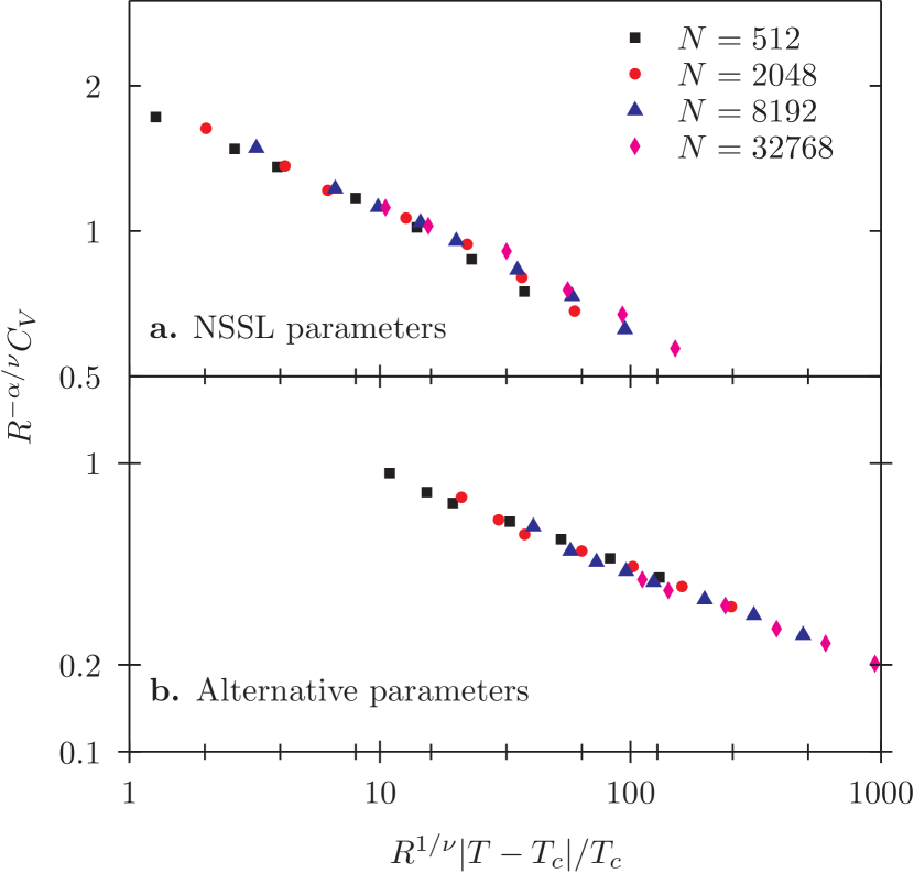
Figure 7: PBCs specific heat scaling plots with two sets of parameters, showing that the scaling is marginal. Top: parameters as in the NSSL scaling (main text), $\nu=1$, $\alpha=0.2$, $T_{c}=0.175$. Bottom: $\nu=0.7$, $\alpha=0.35$, $T_{c}=0.13$.

Appendix F Phase transition and dependence on boundary conditions

We have argued that since in the thermodynamic limit observables must be independent of the boundary conditions unless the system is below a phase transition, our results favor a scenario with a thermodynamic glass transition independently of the particular boundary conditions we have employed. Since our system is already below a phase transition, we expand the argument a bit more, to show how it can safely be extended to a metastable phase.

When a Kauzmann-like transition (i.e. from the supercooled liquid to a phase different from both liquid and crystal) is discussed, it is understood that it involves two metastable phases: the liquid and the ideal glass (or whatever one chooses to call it) are both metastable with respect to the crystal. However, the crystal is usually ignored, implying that one can prove or assume that the time for crystallisation is long enough to allow for the metastable phases to equilibrate before crystallisation begins. Here, we have similarly ignored not only the crystal that eventually forms for very large times, but also the crystalline boundary conditions that would not only select particular crystalline forms, but also greatly accelerate crystallisation.

Recall that boundary conditions are important in the thermodynamic limit when the system is in a broken symmetry phase, where there is coexistence among the different broken-symmetry states (which are themselves connected by an operation of the symmetry that has been broken). To clarify, consider the Ising model below $T_{c}$: the up-down symmetry is broken. This means that the equilibrium state can have positive or negative magnetisation, and that with PBCs both of them will be reached with equal probability. On the other hand, introducing walls with positive (negative) magnetisation will select the state with positive (negative) magnetisation, even in the limit of infinite systems. The phases that coexist are not the paramagnet and the ferromagnet, but the ferromagnetic phases with positive and negative magnetisation. Dependence on the boundary conditions means that there exist boundaries that can select the final state, but there are also boundaries (like PBCs or RBCs) that don’t matter much: the final magnetisation will still be random.

In our case of a liquid below the melting transition, the coexisting phases are the different possible crystals (orientations, shifts, and in general the crystal symmetry operations). A cavity with a crystalline wall would crystallise in the crystal chosen by the wall. But amorphous (i.e. liquid) boundaries are not selecting a particular crystal (rather, they inhibit, though not completely suppress, the crystal).

What we ask is whether the metastable liquid can transition to another phase (also metastable with respect to the solid), and the boundaries we use are noncrystalline: they could select different amorphous states, but with respect to the crystal they are mostly irrelevant (as the RBCs in the Ising example above): for all our boundary conditions, a large enough system crystallises in the long run. If we ignore the crystal (actually, if we are careful to study the system up to the appearance of crystal nuclei, as we do), then we can ask whether there is a symmetry breaking within the metastable state (a metastable liquid-metastable glass transition). Above this transition, the thermodynamic limit must be independent of the boundary conditions, up to the appearance of the crystal (which would be much accelerated if one chose a crystalline border). Below $T_{c}$, the coexisting phases would be e.g. the different states of RFOT (that break the replica symmetry). Our boundary conditions then might select one of those states below $T_{c}$, leading to a dependence on the amorphous boundaries which is not present above $T_{c}$. Again, this ignores a possible crystalline boundary, which would have the same effect above and below $T_{c}$.

References

- Angell (1995) C. A. Angell, Science 267, 1924 (1995).
- Berthier and Biroli (2011) L. Berthier and G. Biroli, Rev. Mod. Phys. 83, 587 (2011).
- Biroli et al. (2008) G. Biroli, J.-P. Bouchaud, A. Cavagna, T. S. Grigera, and P. Verrocchio, Nature Phys. 4, 771 (2008).
- Widmer-Cooper et al. (2008) A. Widmer-Cooper, H. Perry, P. Harrowell, and D. R. Reichman, Nature Phys. 4, 711 (2008).
- Lerner et al. (2009) E. Lerner, I. Procaccia, and J. Zylberg, Physical Review Letters 102, 125701 (2009).
- Tanaka et al. (2010) H. Tanaka, T. Kawasaki, H. Shintani, and K. Watanabe, Nature Mater 9, 324 (2010).
- Sausset and Levine (2011) F. Sausset and D. Levine, Phys. Rev. Lett. 107, 045501 (2011).
- Coslovich (2011) D. Coslovich, Phys. Rev. E 83, 051505 (2011).
- Charbonneau et al. (2012) B. Charbonneau, P. Charbonneau, and G. Tarjus, Phys. Rev. Lett. 108, 035701 (2012).
- Hocky et al. (2012) G. M. Hocky, T. E. Markland, and D. R. Reichman, Phys. Rev. Lett. 108, 225506 (2012).
- Kob et al. (2012) W. Kob, S. Roldán-Vargas, and L. Berthier, Nat. Phys. 8, 164 (2012).
- Ediger (2000) M. D. Ediger, Annu. Rev. Phys. Chem. 51, 99 (2000).
- Sillescu (1999) H. Sillescu, J. Non-Cryst. Sol. 243, 81 (1999).
- Kurchan and Levine (2011) J. Kurchan and D. Levine, J. Phys. A: Math. Theor. 44, 035001 (2011).
- Fernández et al. (2006) L. A. Fernández, V. Martín-Mayor, and P. Verrocchio, Phys. Rev. E 73, 020501 (2006).
- Karmakar et al. (2009) S. Karmakar, C. Dasgupta, and S. Sastry, Proc. Natl. Acad. Sci. USA 106, 3675 (2009).
- Montanari and Semerjian (2006) A. Montanari and G. Semerjian, J. Stat. Phys. 125, 23 (2006).
- Bouchaud and Biroli (2004) J.-P. Bouchaud and G. Biroli, J. Chem. Phys. 121, 7347 (2004).
- Jack and Garrahan (2005) R. L. Jack and J. P. Garrahan, J. Chem. Phys. 123, 164508 (2005).
- Cavagna et al. (2007) A. Cavagna, T. S. Grigera, and P. Verrocchio, Phys. Rev. Lett. 98, 187801 (2007).
- Berthier and Kob (2012) L. Berthier and W. Kob, Phys. Rev. E 85, 011102 (2012).
- Gradenigo et al. (2013) G. Gradenigo, R. Trozzo, A. Cavagna, T. S. Grigera, and P. Verrocchio, J.Chem. Phys. 138, 12A509 (2013).
- Karmakar and Parisi (2013) S. Karmakar and G. Parisi, Proc. Natl. Acad. Sci. 110, 2752 (2013), http://www.pnas.org/content/110/8/2752.full.pdf+html .
- Note (1) Notice that one-time thermodynamic quantities, like energy, density or magnetization, are not sensitive to ABCs Zarinelli and Franz (2010); Cavagna et al. (2010); Krakoviack (2010), while correlation functions and susceptibilities may be.
- Grigera and Parisi (2001) T. S. Grigera and G. Parisi, Phys. Rev. E 63, 045102 (2001).
- Bernu et al. (1987) B. Bernu, J. P. Hansen, Y. Hiwatari, and G. Pastore, Phys. Rev. A 36, 4891 (1987).
- Cavagna et al. (2010) A. Cavagna, T. S. Grigera, and P. Verrocchio, J. Stat. Mech. 2010, P10001 (2010).
- Tanaka (2012) H. Tanaka, Eur. Phys. J. E 35, 113 (2012).
- Cavagna et al. (2012) A. Cavagna, T. S. Grigera, and P. Verrocchio, J. Chem. Phys. 136, 204502 (2012).
- Note (2) See Supplemental Material [url], which includes Refs. Steinhardt et al. (1983); Errington et al. (2003).
- Steinhardt et al. (1983) P. J. Steinhardt, D. R. Nelson, and M. Ronchetti, Phys. Rev. B 28, 784 (1983).
- Errington et al. (2003) J. R. Errington, P. G. Debenedetti, and S. Torquato, J. Chem. Phys. 118, 2256 (2003).
- Rosenfeld and Tarazona (1998) Y. Rosenfeld and P. Tarazona, Mol. Phys. 95, 141 (1998).
- Ingebrigtsen et al. (2013) T. S. Ingebrigtsen, A. A. Veldhorst, T. B. Schrøder, and J. C. Dyre, J. Chem. Phys. 139, 171101 (2013).
- Bolmatov et al. (2012) D. Bolmatov, V. V. Brazhkin, and K. Trachenko, Sci. Rep. 2, 421 (2012).
- Yan et al. (2008) Q. Yan and T. Jain and J. de Pablo , Phys. Rev. Lett. 92, 235701 (2004).
- Zarinelli and Franz (2010) E. Zarinelli and S. Franz, J. Stat. Mech. 2010, P04008 (2010).
- Biroli and Cammarota (2014) G. Biroli and C. Cammarota, “Fluctuations and shape of cooperatively rearranging regions in glass-forming liquids,” arXiv: 1411.4566 (2014).
- Newman and Barkema (1999) M. E. J. Newman and G. Barkema, Monte Carlo Methods in Statistical Physics (Oxford University Press, Oxford, 1999).
- Binney et al. (1992) J. J. Binney, N. J. Dowrick, A. J. Fisher, and M. E. J. Newman, The theory of critical phenomena (Oxford University press, 1992).
- Kirkpatrick and Thirumalai (1987) T. R. Kirkpatrick and D. Thirumalai, Phys. Rev. Lett. 58, 2091 (1987).
- Crisanti and Sommers (1992) A. Crisanti and H.-J. Sommers, Z. Phys. B 87, 341 (1992).
- Coluzzi et al. (1999) B. Coluzzi, M. Mezard, G. Parisi, and P. Verrocchio, J. Chem. Phys. 111, 9039 (1999).
- Lubchenko and Wolynes (2007) V. Lubchenko and P. G. Wolynes, Ann. Rev. Phys. Chem. 58, 235 (2007).
- Kirkpatrick et al. (1989) T. R. Kirkpatrick, D. Thirumalai, and P. G. Wolynes, Phys. Rev. A 40, 1045 (1989).
- Franz (2005) S. Franz, J. Stat. Mech. 2005, P04001 (2005).
- Note (3) It is understood that crystalline boundaries are excluded. This is necessary to remain in the supercooled liquid (a crystalline border would make the whole cavity crystallize). We mean independent from different BCs (such as ABCs, PBCs or RBCs) within the (metastable)liquid phase. See SM for a more complete discussion.
- Parisi (1998) G. Parisi, Statistical Field Theory (Westview Press, 1998).
- Krakoviack (2010) V. Krakoviack, Phys. Rev. E 82, 061501 (2010).