The diameter of a random elliptical cloud

Abstract

We study the asymptotic behavior of the diameter or maximum interpoint distance of a cloud of i.i.d. $d$-dimensional random vectors when the number of points in the cloud tends to infinity. This is a non standard extreme value problem since the diameter is a max $U$-statistic, hence the maximum of dependent random variables. Therefore, the limiting distributions may not be extreme value distributions. We obtain exhaustive results for the Euclidean diameter of a cloud of elliptical vectors whose Euclidean norm is in the domain of attraction for the maximum of the Gumbel distribution. We also obtain results in other norms for spherical vectors and we give several bi-dimensional generalizations. The main idea behind our results and their proofs is a specific property of random vectors whose norm is in the domain of attraction of the Gumbel distribution: the localization into subspaces of low dimension of vectors with a large norm.

Keywords: Elliptical Distributions; Interpoint Distance; Extreme Value Theory; Gumbel Distribution.

AMS Classification (2010): 60D05 60F05

1 Introduction

Let $\{\mathbb{X},\mathbb{X}_{i},i\geq 1\}$ be i.i.d. random vectors in ${\mathbb{R}}^{d}$, for a fixed $d\geq 1$. The quantities of interest in this paper are the maximum Euclidean norm $M_{n}(\mathbb{X})$ and the Euclidean diameter $M_{n}^{(2)}(\mathbb{X})$ of the sample, that is

$$M_{n}(\mathbb{X}) =\max_{1\leq i\leq n}\|\mathbb{X}_{i}\|\;,$$ (1)

$$M_{n}^{(2)}(\mathbb{X}) =\max_{1\leq i<j\leq n}\|\mathbb{X}_{i}-\mathbb{X}_{j}\|\;,$$ (2)

where $\|\cdot\|$ denotes the Euclidean norm in ${\mathbb{R}}^{d}$. The behavior of $M_{n}(\mathbb{X})$ as $n$ tends to infinity is a classical univariate extreme value problem. Its solution is well known. If the distribution of $\|\mathbb{X}\|$ is in the domain of attraction of some extreme value distribution, then $M_{n}(\mathbb{X})$, suitably renormalized, converges weakly to this distribution. We are interested in this paper only in the case where the limiting distribution is the Gumbel law. More precisely, the working assumption of this paper will be that there exist two sequences $\{a_{n}\}$ and $\{b_{n}\}$ such that $\lim_{n\to\infty}a_{n}=\infty$, $\lim_{n\to\infty}b_{n}/a_{n}=0$ and

$$\lim_{n\to\infty}n{\mathbb{P}}(\|\mathbb{X}\|>a_{n}+b_{n}z)=\mathrm{e}^{-z}$$ (3)

for all $z\in{\mathbb{R}}$, or equivalently,

$$\lim_{n\to\infty}{\mathbb{P}}\left(\frac{M_{n}(\mathbb{X})-a_{n}}{b_{n}}\leq z\right)=\mathrm{e}^{-\mathrm{e}^{-z}}\;.$$

The asymptotic behavior of the diameter of the sample cloud is also an extreme value problem since $M_{n}^{(2)}(\mathbb{X})$ is a maximum, but it is a non standard one, because of the dependency between the pairs $(\mathbb{X}_{i},\mathbb{X}_{j})$.

This problem has been recently investigated by [JJ12] for spherically distributed vectors, that is, vectors having the representation $\mathbb{X}=T\mathbb{W}$ where $\mathbb{W}$ is uniformly distributed on the Euclidean unit sphere $\mathcal{S}^{d-1}$ of ${\mathbb{R}}^{d}$ and $T$ is a positive random variable in the domain of attraction of the Gumbel distribution, independent of $\mathbb{W}$. This reference also contains a review of the literature concerning other domains of attractions.

If $d=1$, a spherical random variable is simply a symmetric random variable, that is a positive random variable multiplied by an independent random sign. The diameter of a real valued sample is simply its maximum minus its minimum, and by independence and symmetry, it is straightforward to check that $(M_{n}^{(2)}(\mathbb{X})-2a_{n})/b_{n}$ converges weakly to the sum of two independent Gumbel random variables with location parameter $\log 2$, i.e. distributed as $\Gamma-\log 2$, where $\Gamma$ is a standard Gumbel random variable. Note that the tail of such a sum is heavier than the tail of one Gumbel random variable.

If $d\geq 2$, [JJ12] have shown that in spite of the dependency, the limiting distribution is the Gumbel law, but a correction is needed. Precisely, they proved that if (3) holds, with an additional mild uniformity condition, there exists a sequence $\{d_{n}\}$ such that $d_{n}\to\infty$, $d_{n}=O(\log(a_{n}/b_{n}))$ and

$$\lim_{n\to\infty}{\mathbb{P}}\left(\frac{M_{n}^{(2)}(\mathbb{X})-2a_{n}}{b_{n}}+d_{n}\leq z\right)=\mathrm{e}^{-\mathrm{e}^{-z}}\;.$$ (4)

The exact expression of the sequence $\{d_{n}\}$ will be given in the comments after Theorem 3.2. This implies that $M_{n}^{(2)}(\mathbb{X})/(2M_{n}(\mathbb{X}))$ converges in probability to 1, but the behaviors of $M_{n}(\mathbb{X})$ and $M_{n}^{(2)}(\mathbb{X})$ are subtly different. Specifically, $a_{n}$ is typically a power of $\log n$, so $\log(a_{n}/b_{n})$ is of order $\log\log n$.

It is possible to give some rationale for the presence of the diverging correcting factor $d_{n}$ in (4). In dimension one, two vectors with a large norm may be either on the same side of the origin or on opposite sides. In the latter case their distance is automatically large, typically twice as large as the norm of each one. In higher dimensions, two spherical vectors with a large norm can be close to each other and their distance will be typically much smaller than twice the norm of the largest one. Therefore we expect the probability that the diameter is large to be smaller in the latter case.

This suggests that the asymptotic behavior of the diameter is related to the localization of vectors with large norm. The behavior will differ if large values are to be found in some specific regions of the space or can be found anywhere.

There are many possible directions to extend the results of [JJ12]. One very simple case not covered by these results is the multivariate Gaussian distribution with correlated components. The Gaussian distribution is a particular case of elliptical distributions. The main purpose of this paper is to investigate the behavior of the diameter of a sample cloud of elliptical vectors.

Elliptical vectors are widely used in extreme value theory since they are in the domain of attraction of multivariate extreme value distributions. These distributions and their generalizations have been recently considered in the apparently unrelated problem of obtaining limiting conditional distributions given one component is extreme, see [FS10] and the references therein.

In this paper, the tail behavior of a product $TU$, where $T$ is in the domain of attraction of the Gumbel distribution and $U$ is a bounded positive random variable independent of $T$, was obtained as a by-product of the main result. Under some regularity assumption on the density of $U$ at its maximum, the tail of $TU$ is slightly lighter than the tail of $T$. The main reason is that if a random variable $T$ is in the domain of attraction of the Gumbel distribution, then for any $\alpha>1$,

$$\lim_{x\to\infty}\frac{{\mathbb{P}}(T>\alpha x)}{{\mathbb{P}}(T>x)}=0\;.$$

This implies that for $TU$ to be large, $U$ must be very close to its maximum. The full strength of this remark was recently exploited in [BS13] who obtained the rate of convergence of $U$ towards its maximum when the product $TU$ is large and the conditional limiting distribution of the difference between $U$ and its maximum, suitably renormalized. This property explains deeply the conditional limits obtained in [FS10]. Having in mind the earlier remarks on the link between the localization of the vectors with large norm and the asymptotic distribution of the diameter, it is clear that this localization property will be helpful to study the problem at hand in this paper.

The rest of the paper is organized as follows. In Section 2, we will define elliptical vectors and state our main results. In section 2.1, extending the results of [BS13], we will show that the realizations of a $d$-dimensional random elliptical vector with large norm are localized on a subspace of ${\mathbb{R}}^{d}$ whose dimension is the multiplicity of the largest eigenvalue of the covariance matrix. This result will be crucial to prove our main results which are stated in Section 3. As partially conjectured by [JJ12, Section 5.4], if the largest eigenvalue of the covariance matrix is simple, then the limiting distribution of the diameter is similar but not equal to the one which arises when $d=1$: correcting terms appear that are due the fluctuations around the direction of the largest eigenvalue. If the largest eigenvalue is not simple, say its multiplicity is $k$, then the diameter behaves as in the spherical case in dimension $k$, up to constants.

In Section 4, we will answer another question of [JJ12], namely we will investigate the $l^{q}$ diameter of a cloud of spherical vectors, for $1\leq q\leq\infty$. This problem is actually simpler than the corresponding one in Euclidean ($l^{2}$) norm, since the vectors with large norm are always localized close to a finite number of directions. Therefore, the “localization principle” applies and we obtain the same type of limiting distribution as in the case of an elliptical distribution with simple largest eigenvalue. For $q=1$ and $q>2$ the problem simplifies even further since the corrective terms vanish and the limiting distribution of the one dimensional case is obtained.

In Section 5, we discuss further possible generalizations and give several bidimensional examples.

We think that beyond answering certain questions on the diameter of a random cloud, the main purpose of this paper is to emphasize the use of the localization principle of vectors with large norm in the domain of attraction of the Gumbel distribution. This principle should be useful in other problems.

2 The Euclidean norm of an elliptical vector

A random vector $\mathbb{X}$ in ${\mathbb{R}}^{d}$ has an elliptical distribution if it can be expressed as

$$\mathbb{X}=TA\mathbb{W}$$ (5)

where $T$ is a positive random variable, $A$ is an invertible $d\times d$ matrix and $\mathbb{W}=(W_{1},\dots,W_{d})$ is uniformly distributed on the sphere $\mathcal{S}^{d-1}$. The covariance matrix of $\mathbb{X}$ is then given by ${\mathbb{E}}[T^{2}]A^{\prime}A$ where $M^{\prime}$ denotes the transpose of any matrix $M$. Let $\lambda_{1}\geq\dots\geq\lambda_{d}>0$ be its ordered eigenvalues repeated according to their multiplicity. The distribution is spherical if all the eigenvalues are equal. Otherwise, there exists $k\in\{1,\dots,d-1\}$ such that

$$\lambda_{1}=\cdots=\lambda_{k}>\lambda_{k+1}\;.$$ (6)

We will see that this number $k$ plays a crucial role for tail of the norm and the asymptotic distribution of the diameter.

Let $\mathbb{W}_{i}=(W_{i,1},\dots,W_{i,d})$, $i=1,2$, be independent random vectors uniformly distributed on $\mathcal{S}^{d-1}$, and define $\mathbb{X}_{i}=T_{i}A\mathbb{W}_{i}$, which are i.i.d. with the same distribution as $\mathbb{X}$. Since for any orthogonal matrix $P$ (i.e. $P^{\prime}=P^{-1}$), $P\mathbb{W}$ is also uniformly distributed on $\mathcal{S}^{d-1}$, it holds that

$$\|\mathbb{X}\|^{2} \stackrel{{\scriptstyle(d)}}{{=}}T^{2}\sum_{q=1}^{d}\lambda_{q}W_{q}^{2}\;,$$

$$\|\mathbb{X}_{1}-\mathbb{X}_{2}\|^{2} \stackrel{{\scriptstyle(d)}}{{=}}T^{2}\sum_{q=1}^{d}\lambda_{q}(W_{1,q}-W_{2,q})^{2}\;,$$

where $\stackrel{{\scriptstyle(d)}}{{=}}$ denotes equality in law. Define

$$\mathbb{Y}=T(\sqrt{\lambda_{1}}W_{1},\dots,\sqrt{\lambda_{d}}W_{d})$$ (7)

and let $\{\mathbb{Y}_{i},i\geq 1\}$ is a sequence of i.i.d. vectors with the same distribution as $\mathbb{Y}$. Then

$$M_{n}(\mathbb{X})\stackrel{{\scriptstyle(d)}}{{=}}M_{n}(\mathbb{Y})\;,\ \ M_{n}^{(2)}(\mathbb{X})\stackrel{{\scriptstyle(d)}}{{=}}M_{n}^{(2)}(\mathbb{Y})\;.$$

Therefore, we will prove our results using the vectors $\{\mathbb{Y}_{i},i\geq 1\}$.

In all the sequel, we will assume that $T$ is in the max domain of attraction of the Gumbel law, i.e. the limit (3) holds, or equivalently, there exists a function $\psi_{T}$, called an auxiliary function for $T$, defined on $(0,\infty)$ such that

$$\lim_{x\to\infty}\frac{\psi_{T}(x)}{x}=0\;,$$

and

$$\lim_{x\to\infty}\frac{{\mathbb{P}}(T>x+\psi_{T}(x)z)}{{\mathbb{P}}(T>x)}=\mathrm{e}^{-z}\;,$$ (8)

locally uniformly with respect to $z\in{\mathbb{R}}$. Moreover, the survival function of $T$ can be expressed as

$${\mathbb{P}}(T>x)=\vartheta(x)\exp\left(-\int_{x_{0}}^{x}\frac{\mathrm{d}s}{\psi_{T}(s)}\right)\;,$$ (9)

where $\lim_{x\to\infty}\vartheta(x)\in(0,\infty)$. See e.g. [Res87, Chapter 0].

Define the functions $\psi_{A}$ and $\phi_{A}$ on $(0,\infty)$ by

$$\psi_{A}(x) =\sqrt{\lambda_{1}}\psi_{T}(x/\sqrt{\lambda_{1}})\;,\ \ \ \phi_{A}(x)=\sqrt{\frac{\psi_{T}(x/\sqrt{\lambda_{1}})}{x/\sqrt{\lambda_{1}}}}=\sqrt{\psi_{A}(x)/x}\;.$$

In the sequel, the notation $\sim$ means that the ratio of the two terms around $\sim$ tend to one when their parameter ($x$ or $n$) tends to infinity and $\ \stackrel{{\scriptstyle{\rm(d)}}}{{\longrightarrow}}\$ denotes weak convergence of probability distribution.

Theorem 2.1.

Let $\mathbb{X}$ be as in (5) with $T$ satisfying (8), $\mathbb{W}$ uniformly distributed on $\mathcal{S}^{d-1}$, and assume that the eigenvalues $\lambda_{1},\dots,\lambda_{d}$ of the correlation matrix satisfy (6). Then,

$${\mathbb{P}}(\|\mathbb{X}\|>x) \sim\frac{\Gamma(\frac{d}{2})}{\Gamma(\frac{k}{2})}2^{(d-k)/2}\;\left(\prod_{q=k+1}^{d}\frac{\lambda_{1}}{\lambda_{1}-\lambda_{q}}\right)^{1/2}\;\phi_{A}^{d-k}(x)\;{\mathbb{P}}(T>x/\sqrt{\lambda_{1}})\;.$$

Let $\mathbb{Y}$ be as in (7). Then, as $x\to\infty$, conditionally on $\|\mathbb{Y}\|>x$,

$$\left(\tfrac{\|\mathbb{Y}\|-x}{\psi_{A}(x)},W_{1},\dots,W_{k},\tfrac{W_{k+1}}{\phi_{A}(x)},\dots,\tfrac{W_{d}}{\phi_{A}(x)}\right)\ \stackrel{{\scriptstyle{\rm(d)}}}{{\longrightarrow}}\ (E,\mathbb{W}^{(k)},\sqrt{\tfrac{\lambda_{1}}{\lambda_{1}-\lambda_{k+1}}}G_{k+1},\dots,\sqrt{\tfrac{\lambda_{1}}{\lambda_{1}-\lambda_{d}}}G_{d})\;,$$

where $E$ is an exponential random variable with mean 1, $\mathbb{W}^{(k)}$ is uniformly distributed on $\mathcal{S}^{k-1}$, $G_{k+1},\dots,G_{d}$ are independent standard Gaussian random variables, and all components are independent.

Comments

• This result implies that $\|\mathbb{X}\|$ is in the domain of attraction of the Gumbel distribution and that an auxiliary function for $\|\mathbb{X}\|$ is $\psi_{A}$.

• The first statement can be obtained as a consequence of [FS10, Proposition 3.2.1]. In dimension 2, the second result is a consequence of [BS13, Theorem 2.1], where a real valued random variable $X$ which can be expressed $X=Tu(S)$ is considered, with $T$ satisfying (9), $S$ taking values in $[0,1]$ and the bounded function $u$ having some regularity properties around its maximum and the asymptotic behavior of $S$ conditionally on the product $Tu(S)$ being large is obtained.

We now consider the polar representation of the vector $\mathbb{Y}$, that is we define $\Theta=\frac{\mathbb{Y}}{\|\mathbb{Y}\|}$ and for $q=k+1,\dots,d$, we define also $\tau_{q}^{2}={\frac{\lambda_{q}}{\lambda_{1}-\lambda_{q}}}$.

Corollary 2.2.

Under the conditions of Theorem 2.1, as $x\to\infty$, conditionally on $\|\mathbb{Y}\|>x$,

$$\left(\tfrac{\|\mathbb{Y}\|-x}{\psi_{A}(x)},\Theta_{1},\dots,\Theta_{k},\tfrac{\Theta_{k+1}}{\phi_{A}(x)},\dots,\tfrac{\Theta_{d}}{\phi_{A}(x)}\right)\ \stackrel{{\scriptstyle{\rm(d)}}}{{\longrightarrow}}\ (E,\mathbb{W}^{(k)},\tau_{k+1}G_{k+1},\dots,\tau_{d}G_{d})\;,$$

where $E$ is an exponential random variable with mean 1, $\mathbb{W}^{(k)}$ is uniformly distributed on $\mathcal{S}^{k-1}$, $G_{k+1},\dots,G_{d}$ are independent standard Gaussian random variables, and all components are independent.

This result can be rephrased in terms of weak convergence of point processes (see e.g. [Res87, Proposition 3.21]). Let $a_{n}$ be the $1-1/n$ quantile of the distribution of $\|\mathbb{X}\|$ or $\|\mathbb{Y}\|$, i.e. ${\mathbb{P}}(\|\mathbb{X}\|>a_{n})={\mathbb{P}}(\|\mathbb{Y}\|>a_{n})\sim 1/n$ and set $b_{n}=\psi_{A}(a_{n})$ and $c_{n}=\phi_{A}(a_{n})$. Define the points

$$P_{n,i}=\left(\frac{\|\mathbb{Y}_{i}\|-a_{n}}{b_{n}},\Theta_{1},\dots,\Theta_{k},\frac{\Theta_{k+1}}{c_{n}},\dots,\frac{\Theta_{d}}{c_{n}}\right)\;.$$ (10)

Corollary 2.3.

Under the conditions of Theorem 2.1, the point processes $\sum_{i=1}^{n}\delta_{P_{n,i}}$ converge weakly to a Poisson point process $N=\sum_{i=1}^{\infty}\delta_{P_{i}}$ on ${\mathbb{R}}\times\mathcal{S}^{k-1}\times{\mathbb{R}}^{d-k}$ with

$$P_{i}=(\Gamma_{i},\mathbb{W}^{(k)}_{i},\tau_{k+1}G_{i,k+1},\dots,\tau_{d}G_{i,d})\;,$$ (11)

where $\{\Gamma_{i},i\geq 1\}$ are the points of a Poisson point process on $(-\infty,\infty]$ with mean measure $\mathrm{e}^{-x}\mathrm{d}x$, $\{\mathbb{W}^{(k)}_{i},i\geq 1\}$ are i.i.d. vectors uniformly distributed on $\mathcal{S}^{k-1}$ and $\{G_{i,q},i\geq 1,q=k+1,\dots,d\}$ are i.i.d. standard Gaussian variables, all sequences being mutually independent.

Comments

Since the measure $\mathrm{e}^{-x}\,\mathrm{d}x$ is finite on any interval $[a,\infty]$, $a\in{\mathbb{R}}$, the point process $N$ has a finite number of points on any set $[a,\infty]\times\mathcal{S}^{d-1}\times{\mathbb{R}}^{d-k}$. Therefore, the points can and will be numbered in such a way that $\Gamma_{1}>\Gamma_{2}>\dots$. Moreover, if the points $P_{n,i}$ are also numbered in decreasing order of their first component, then for each fixed integer $m$, $(P_{n,1},\dots,P_{n,m})$ converges weakly to $(P_{1},\dots,P_{m})$.

We illustrate Theorem 2.1 for three dimensional Gaussian vectors whose maximum eigenvalue $\lambda_{1}$ of the correlation matrix is simple (Figure 1a) or double (Figure 1b). The rate of convergence to zero of the coordinates corresponding to the smallest eigenvalues is $O(\log n)$.

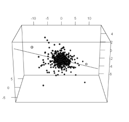
(a) $\lambda_{1}=4$, $\lambda_{2}=1$, $\lambda_{3}=0.5$

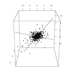
(b) $\lambda_{1}=\lambda_{2}=4$, $\lambda_{3}=0.5$

Figure 1: Two sample clouds of size $1000$ of the trivariate Gaussian distribution. The eigenvalues of the correlation matrix are given under each figure. The gray spheres are the points which realize the diameter. The black lines are the principal axes.

Proof of Theorem 2.1

We will need the following Lemma.

Lemma 2.4.

Let $\mathbb{W}$ be uniformly distributed on $\mathcal{S}^{d-1}$. For $k\in\{1,\dots,d-1\}$, define the random vector $\mathbb{W}^{(k)}$ on $\mathcal{S}^{k}$ by

$$\mathbb{W}^{(k)}=\frac{1}{\sqrt{1-W_{k+1}^{2}-\cdots-W_{d}^{2}}}(W_{1},\dots,W_{k})\;.$$

Then $\mathbb{W}^{(k)}$ is uniformly distributed on $\mathcal{S}^{k}$ and independent of $(W_{k+1},\dots,W_{d})$. If $f$ is continuous and compactly supported on ${\mathbb{R}}^{d}$, then

$$\lim_{s\to\infty}s^{d-k}\,{\mathbb{E}}[f(W_{1},\dots,W_{k},sW_{k+1},\dots,sW_{d})]\\ =\frac{\Gamma(\frac{d}{2})}{\pi^{\frac{d-k}{2}}\Gamma(\frac{k}{2})}\int_{{\mathbb{R}}^{k}}{\mathbb{E}}[f(\mathbb{W}^{(k)},t_{k+1},\dots,t_{d})]\,\mathrm{d}t_{k+1}\dots\mathrm{d}t_{d}\;.$$ (12)

The convergence (12) can be extended to sequences of continuous functions $f_{x}$ with compact support which depend on $x$ provided they converge locally uniformly to a continuous function with compact support. By bounded convergence, it can also be extended to sequences of bounded continuous functions $f_{x}$ if there exists a function $f^{*}$ (not depending on $x$) and such that $|f_{x}|\leq f^{*}$ for all $x$ and $\int_{{\mathbb{R}}^{k}}{\mathbb{E}}[f^{*}(\mathbb{W}^{(k)},t_{k+1},\dots,t_{d})]\,\mathrm{d}t_{k+1}\dots\mathrm{d}t_{d}<\infty$. The proof of the Lemma consists merely in a change of variable and is postponed to Section 6.

Proof of Theorem 2.1.

Note first that if $(w_{1},\dots,w_{d})\in\mathcal{S}^{d-1}$, then

$$\sum_{q=1}^{d}\lambda_{q}w_{q}^{2}=\lambda_{1}\left(1-\sum_{q=k+1}^{d}\gamma_{q}^{-2}w_{q}^{2}\right)\;,$$

with $\gamma_{q}^{2}=\lambda_{1}/(\lambda_{1}-\lambda_{q})$, $q=k+1,\dots,d$. Thus we can write

$$\|\mathbb{Y}\|=\sqrt{\lambda_{1}}T-\sqrt{\lambda_{1}}Tg(W_{k+1},\dots,W_{d})\;,$$

where

$$g(w_{k+1},\dots,w_{d}) =1-\sqrt{1-\sum_{q=k+1}^{d}\gamma_{q}^{-2}w_{q}^{2}}\;,$$

and

$$\lim_{s\to\infty}s^{2}g(s^{-1}w_{k+1},\dots,s^{-1}w_{d}) =\frac{1}{2}\sum_{q=k+1}^{d}\gamma_{q}^{-2}w_{q}^{2}\;,$$

locally uniformly with respect to $w_{k+1},\dots,w_{d}$.

For $x>0$, define the function $k_{x}$ on ${\mathbb{R}}^{d-k+1}$ by

$$k_{x}(z,w_{k+1},\dots,w_{d}) =\frac{{\mathbb{P}}\left(\|\mathbb{X}\|>x+\psi_{A}(x)z\mid W_{q}=\phi_{A}(x)w_{q},q=k+1,\dots,d\right)}{{\mathbb{P}}(T>x/\sqrt{\lambda_{1}})}$$

$$=\frac{{\mathbb{P}}\left(T>\frac{x/\sqrt{\lambda_{1}}\;+\;\psi_{T}(x/\sqrt{\lambda_{1}})z}{1-g(\phi_{A}(x)w_{k+1},\dots,\phi_{A}(x)w_{d})}\right)}{{\mathbb{P}}(T>x/\sqrt{\lambda_{1}})}\;.$$

Since we have defined $\phi_{A}$ such that $x\phi_{A}^{2}(x)=\sqrt{\lambda_{1}}\psi_{T}(x/\sqrt{\lambda_{1}})$, we obtain that

$$\lim_{x\to\infty}k_{x}(z,w_{k+1},\dots,w_{d})=\exp\bigg{(}-z-\frac{1}{2}\sum_{q=k+1}^{d}\gamma_{q}^{-2}w_{q}^{2}\bigg{)}\;,$$

locally uniformly with respect to $z,w_{k+1},\dots,w_{d}$. Let $f$ be a continuous function with compact support in ${\mathbb{R}}^{d}$. Applying Lemma 2.4, we obtain

$$\lim_{x\to\infty} \frac{1}{\phi_{A}^{k-d}(x){\mathbb{P}}(T>x/\lambda_{1})}{\mathbb{E}}\left[f\left(W_{1},\dots,W_{k},\tfrac{W_{k+1}}{\phi(x)},\dots,\tfrac{W_{k+1}}{\phi(x)}\right)\mathbbm{1}_{\{\|\mathbb{Y}\|>x+\psi_{A}(x)z\}}\right]$$

$$=\lim_{x\to\infty}\phi_{A}^{k-d}(x){\mathbb{E}}\left[f\left(W_{1},\dots,W_{k},\tfrac{W_{k+1}}{\phi(x)},\dots,\tfrac{W_{k+1}}{\phi(x)}\right)k_{x}\left(z,\tfrac{W_{k+1}}{\phi_{A}(x)},\dots,\tfrac{W_{d}}{\phi_{A}(x)}\right)\right]$$

$$=\frac{\Gamma(\frac{d}{2})}{\pi^{(d-k)/2}\Gamma(\frac{k}{2})}\;\mathrm{e}^{-z}\,\int_{{\mathbb{R}}^{d-k}}{\mathbb{E}}[f(\mathbb{W}^{(k)},t_{k+1},\dots,t_{d})]\,\mathrm{e}^{-\frac{1}{2}\sum_{q=k+1}^{d}\gamma_{q}^{-2}w_{q}^{2}}\,\mathrm{d}t_{k+1}\dots\mathrm{d}t_{d}$$

$$=\frac{\Gamma(d/2)}{\Gamma(k/2)}2^{({d-k})/2}\;\prod_{q=k+1}^{d}\gamma_{q}\;\mathrm{e}^{-z}\,{\mathbb{E}}[f(\mathbb{W}^{(k)},\gamma_{k+1}G_{k+1},\dots,\gamma_{d}G_{d})]\;,$$ (13)

where $G_{k+1},\dots,G_{d}$ are i.i.d. standard Gaussian random variables.

The last step is to extend the convergence (13) to all bounded continuous functions $f$. By the comments after Lemma 2.4, it suffices to prove that the function $k_{x}$ can be bounded by a function $k^{*}$ independent of $x$ and integrable with respect to Lebesgue’s measure on ${\mathbb{R}}^{d-k}$. For any $u\geq 0$ and $p>0$, there exists a constant $C$ such that, for large enough $x$,

$$\frac{{\mathbb{P}}(T>x+\psi_{T}(x)u)}{{\mathbb{P}}(T>x)}\leq C(1+u)^{-p}\;,$$ (14)

(see e.g. [FS10, Lemma 5.1]). For $z\geq 0$, this trivially yields

$$\frac{{\mathbb{P}}(T>x+\psi_{T}(x)(z+u))}{{\mathbb{P}}(T>x)}\leq C(1+u)^{-p}\;.$$ (15)

For a fixed $z<0$, we write

$$\frac{{\mathbb{P}}(T>x+\psi_{T}(x)(z+u))}{{\mathbb{P}}(T>x)}=\frac{{\mathbb{P}}(T>x+\psi_{T}(x)z)}{{\mathbb{P}}(T>x)}\frac{{\mathbb{P}}(T>x+\psi_{T}(x)z+\psi_{T}(x)u)}{{\mathbb{P}}(T>x+\psi_{T}(x)z)}\;.$$

The first ratio in the right hand side is convergent hence bounded and since $z$ is fixed, we can apply the bound (14) to the second ratio, upon noting that $\lim_{x\to\infty}\psi_{T}(x+\psi_{T}(x)z)/\psi_{T}(x)=1$ for all $z\in{\mathbb{R}}$. Thus (15) also holds with a constant $C$ uniform with respect to $z$ in compact sets of $(-\infty,0]$.

Since

$$\frac{1}{1-g(w_{k+1},\dots,w_{d})}\geq 1+\frac{1}{2}\sum_{q=k+1}^{d}\gamma_{q}^{-2}w_{q}^{2}\;,$$

we obtain, applying (15) with $u=\frac{1}{2}\sum_{q=k+1}^{d}\gamma_{q}^{-2}w_{q}^{2}$ and a fixed $z\in{\mathbb{R}}$,

$$k_{x}(z,w_{k+1},\dots,w_{d})\leq\frac{{\mathbb{P}}\left(T>x/\sqrt{\lambda_{1}}+\psi_{T}(x/\sqrt{\lambda_{1}})(z+u)\right)}{{\mathbb{P}}(T>x/\sqrt{\lambda_{1}})}\leq C(1+u)^{-p}\;.$$

For $p$ large enough, the function $k^{*}(w_{1},\dots,w_{d})=\left(1+\frac{1}{2}\sum_{q=k+1}^{d}\gamma_{q}^{-2}w_{q}^{2}\right)^{-p}$ is integrable with respect to Lebesgue’s measure on ${\mathbb{R}}^{d-k}$. This concludes the proof. ∎

3 Asymptotic behavior of the Euclidean diameter

We now study the behavior of the diameter of the elliptical cloud $\{\mathbb{X}_{i},1\leq i\leq n\}$. Precisely, we investigate the asymptotic behavior of $(M_{n}^{(2)}(\mathbb{X})-2a_{n})/b_{n}$ in the case $k=1$ and $k>1$. As previously, we will prove our results with the vectors $\mathbb{Y}_{i}$, $i\geq 1$.

3.1 Case $k=1$: single maximum eigenvalue

In this case, the points $P_{n,i}$ defined in (10) become

$$P_{n,i}=\left(\frac{\|\mathbb{Y}_{i}\|-a_{n}}{b_{n}},\Theta_{1},\frac{\Theta_{2}}{c_{n}},\dots,\frac{\Theta_{d}}{c_{n}}\right)\;.$$

By Corollary 2.3, $N_{n}=\sum_{i=1}^{n}\delta_{P_{n,i}}$ converges weakly to a Poisson point process $N=\sum_{i=1}^{\infty}\delta_{P_{i}}$ on ${\mathbb{R}}\times\{-1,1\}\times{\mathbb{R}}^{d-1}$ with $P_{i}=(\Gamma_{i},\varepsilon_{i},\tau_{2}G_{i,2},\dots,\tau_{d}G_{i,d})$, where $\varepsilon_{i}$, $i\geq 1$ are i.i.d. symmetric random variables with values in $\{-1,+1\}$ and the other components are as in Corollary 2.3.

By the independent increment property of the Poisson point process, the point process $N$ can be split into two independent Poisson point processes $N^{+}$ and $N^{-}$ on ${\mathbb{R}}^{d}$ whose points are the points of $N$ with second component equal to $+1$ or $-1$ respectively. The mean measure of both processes is $\frac{1}{2}\mathrm{e}^{-x}\,\mathrm{d}x\,\Phi_{\tau_{2}}(\mathrm{d}t_{2})\cdots\Phi_{\tau_{d}}(\mathrm{d}t_{d})$.

Then the point processes $N_{n}^{+}$ and $N_{n}^{-}$ defined by

$$N_{n}^{+}=\sum_{i=1}^{n}\delta_{P_{n,i}}\mathbbm{1}_{\{\Theta_{i,1}>0\}}\;,\ \ N_{n}^{-}=\sum_{i=1}^{n}\delta_{P_{n,i}}\mathbbm{1}_{\{\Theta_{i,1}<0\}}\;,$$

converge weakly to the independent point processes $N^{+}$ and $N^{-}$ on ${\mathbb{R}}^{d}$ which can be expressed as

$$N^{\pm}=\sum_{i=1}^{\infty}\delta_{(\Gamma_{i}^{\pm},\tau_{2}G_{i,2}^{\pm},\dots,\tau_{d}G_{i,d}^{\pm})}\;,$$

where $\{\Gamma_{i}^{\pm},i\geq 1\}$ are the points of a Poisson point process with mean measure $\frac{1}{2}\mathrm{e}^{-x}\mathrm{d}x$ on ${\mathbb{R}}$, and $\{G_{i,q}^{\pm}$, $i\geq 1$, $q=2,\dots,d\}$ are i.i.d. standard Gaussian variables, independent of the points $\{\Gamma_{i}^{\pm},i\geq 1\}$.

Since the mean measure is finite on the half planes $(x,\infty]\times[-\infty,\infty]$, there is almost surely a finite number of points of $N^{\pm}$ in any of these half planes. Thus, the points of $N^{\pm}$ can and will be numbered in decreasing order of their first component.

We can now state the main result of this section.

Theorem 3.1.

Let $\{\mathbb{X}_{i},i\geq 1\}$ be a sequence of i.i.d. random vectors with the same distribution as $\mathbb{X}$ and let the assumptions of Theorem 2.1 hold with $k=1$, i.e. $\lambda_{1}>\lambda_{2}$, then

$$\frac{M_{n}^{(2)}(\mathbb{X})-2a_{n}}{b_{n}}\ \stackrel{{\scriptstyle{\rm(d)}}}{{\longrightarrow}}\ \max_{i,j\geq 1}\left\{\Gamma_{i}^{+}+\Gamma_{j}^{-}-\frac{1}{4}\sum_{q=2}^{d}\frac{\lambda_{q}}{\lambda_{1}-\lambda_{q}}(G_{i,q}^{+}-G_{j,q}^{-})^{2}\right\}\;,$$ (16)

where $\{(\Gamma_{i}^{+},G_{i,2}^{+},\dots,G_{i,d}^{+}),i\geq 1\}$ and $\{(\Gamma_{i}^{-},G_{i,2}^{-},\dots,G_{i,d}^{-}),i\geq 1\}$ are the points of two independent point processes with mean measure $\frac{1}{2}\mathrm{e}^{-x}\mathrm{d}x\Phi(\mathrm{d}t_{2})\dots\Phi(\mathrm{d}t_{d})$.

Comments

The random variable defined in (16) is almost surely finite, since it is upper bounded by $\Gamma_{1}^{+}+\Gamma_{1}^{-}$. The lower bound $\Gamma_{1}^{+}+\Gamma_{1}^{-}-\frac{1}{4}\sum_{q=2}^{d}\tfrac{\lambda_{q}}{\lambda_{1}-\lambda_{q}}(G_{1,q}^{+}-G_{1,q}^{-})^{2}$ trivially holds. These two bounds imply that the limiting distribution is tail equivalent to the sum of two independent Gumbel random variables which is heavier tailed than a Gumbel distribution. However, it is not the sum of two independent Gumbel random variables. Therefore this result is different from the result in the spherical case in any dimension.

3.1.1 Case of the dimension 2

In dimension 2, a bivariate elliptical random vector $\mathbb{X}$ with correlation $\rho\in(0,1)$ can be defined by

$$\mathbb{X}=T(\cos U,\rho\cos U+\sqrt{1-\rho^{2}}\sin U)=T(\cos U,\cos(U-U_{0}))\;,$$

where $U$ is uniformly distributed on $[0,2\pi]$, $\cos U_{0}=\rho$ and $\sin U_{0}=\sqrt{1-\rho^{2}}$. The vector $\mathbb{X}$ admits the polar representation $\mathbb{X}=R(\cos\Theta,\sin\Theta)$ with

$$R =T\sqrt{1+\rho\cos(2U-U_{0})}\;,$$

$$\cos\Theta =\frac{\cos U}{\sqrt{1+\rho\cos(2U-U_{0})}}\;,\sin\Theta=\frac{\cos(U-U_{0})}{\sqrt{1+\rho\cos(2U-U_{0})}}\;.$$

The correlation matrix of $\mathbb{X}$ is then

$$\begin{pmatrix}1&\rho\\ \rho&1\end{pmatrix}\;.$$

Its eigenvalues are $1+\rho$ and $1-\rho$. By Theorem 2.1, we know that $\|\mathbb{X}\|$ is in the domain of attraction of the Gumbel law and more precisely, as $x\to\infty$,

$${\mathbb{P}}(\|\mathbb{X}\|>x\sqrt{1+\rho})\sim\sqrt{\frac{1+\rho}{\pi\rho}}\sqrt{\frac{\psi_{T}(x)}{x}}{\mathbb{P}}\left(T>x\right)\;.$$

Note that $(1,1)$ is always an eigenvector associated with the eigenvalue $1+\rho$. This means that the vectors in the cloud with large norm are localized close to the diagonal, whatever the value of $\rho\in(0,1)$. More precisely, let $\widetilde{\Theta}_{n}$ be the angle of the point $\widetilde{\mathbb{X}}_{n}$ of the cloud $\{\mathbb{X}_{i},1\leq i\leq n\}$ such that $\|\widetilde{\mathbb{X}}_{n}\|=M_{n}(\mathbb{X})$. Then $(\widetilde{\Theta}_{n}-\tfrac{\pi}{4}-\pi\mathbbm{1}_{\{\cos\widetilde{\Theta}_{n}<0\}})/c_{n}$ converges weakly to a Gaussian variable with mean zero and variance $(1-\rho)/2\rho$.

By Theorem 3.1, the limiting distribution of the diameter can be expressed as

$$\max_{i,j\geq 1}\left\{\Gamma_{i}^{+}+\Gamma_{j}^{-}-\frac{1-\rho}{8\rho}(G_{i}^{+}-G_{j}^{-})^{2}\right\}\;,$$ (17)

where $\{(\Gamma_{i}^{+},G_{i}^{+}),i\geq 1\}$ and $\{(\Gamma_{i}^{-},G_{i}^{-}),i\geq 1\}$ are the points of two independent point processes with mean measure $\frac{1}{2}\mathrm{e}^{-x}\mathrm{d}x\Phi(\mathrm{d}t)$. If $\rho=1$, the one dimensional case is recovered, but there is a discontinuity with the spherical case $\rho=0$ where the limiting distribution is Gumbel and the normalization is different. Moreover, if $\hat{\mathbb{X}}_{n}$ and $\check{\mathbb{X}}_{n}$ are the points such that $\|\hat{\mathbb{X}}_{n}-\check{\mathbb{X}}_{n}\|=M_{n}^{(2)}(\mathbb{X})$, if $\hat{\Theta}_{n}$ and $\check{\Theta}_{n}$ are their respective angle such that $\cos\hat{\Theta}_{n}>0$, $\cos\check{\Theta}_{n}<0$, then $((\hat{\Theta}_{n}-\pi/4)/c_{n},(\check{\Theta}_{n}-5\pi/4)/c_{n})$ converges weakly to a pair of i.i.d. Gaussian random variables with mean zero and variance $(1-\rho)/2\rho$.

(a) $\rho=0.2$

(b) $\rho=0.8$

Figure 2: Two bidimensional Gaussian clouds. The black triangles are the points which realize the diameter. The black line is the diagonal and the dotted line is the regression line $y=\rho x$. The ellipses are the level lines of the density of the Gaussian distribution.

In Figure 2 we show two sample clouds of size $1000$ of bivariate Gaussian variables with correlation $\rho=0.2$ and $\rho=0.8$. The rate of convergence to the diagonal is $O(\log n)$. In Figure 3, we show the empirical cumulative distribution function (cdf) of the limiting distribution based on 500 replications of the diameter of a Gaussian cloud (with correlation $\rho=0.2$) of size 100 000. In simulations, the indices realizing the maximum in (17) are often $i=1$ and $j=1$. This implies that the limiting distribution of the diameter should be close to the distribution of the sum of two independent Gumbel random variables minus the square of a Gaussian random variable. We show this distribution together with the empirical and theoretical cdf of the diameter in Figure 3.

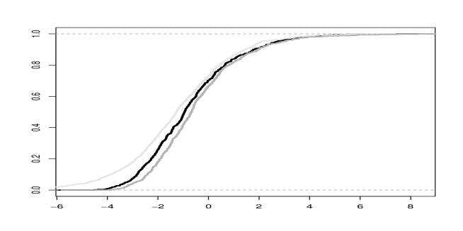
Figure 3: Distribution function of the limiting distribution of the diameter of a bidimensional elliptical cloud. The black thick line is the (simulated) theoretic cdf; the thick gray line is the empirical cdf based on 500 clouds of 100 000 points. The thin gray line is the cdf of the sum of two independent Gumbel random variables with location parameter $\log 2$.

3.1.2 Proof of Theorem 3.1

Define the set $O_{n}=\{w\in{\mathbb{R}}^{d-1}\mid c_{n}^{2}\|w\|^{2}\leq 1\}$ and the function $f_{n}$ on ${\mathbb{R}}\times\{-1,+1\}\times O_{n}\to{\mathbb{R}}^{d}$ by

$$f_{n}(r,\epsilon,w)=(a_{n}+b_{n}r)(\epsilon\sqrt{1-c_{n}^{2}\|w\|^{2}},c_{n}w)\;.$$

Define next the function $g_{n}$ on ${\mathbb{R}}\times\{-1,+1\}\times O_{n}\times{\mathbb{R}}\times\{-1,+1\}\times O_{n}$ by

$$g_{n}(r_{1},\epsilon_{1},w_{1},r_{2},\epsilon_{2},w_{2})=\frac{\|f_{n}(r_{1},\epsilon_{1},w_{1})-f_{n}(r_{2},\epsilon_{2},w_{2})\|-2a_{n}}{b_{n}}\;.$$

Since $c_{n}\to 0$, any $w\in{\mathbb{R}}^{d-1}$ is in $O_{n}$ for all large enough $n$. Then, for any $r_{1},r_{2}>0$, for $\epsilon_{1},\epsilon_{2}\in\{-1,1\}$ and any $w_{1},w_{2}\in{\mathbb{R}}^{d-1}$,

$$\lim_{n\to\infty}g_{n}(r_{1},\epsilon_{1},w_{1},r_{2},\epsilon_{2},w_{2}) =g(r_{1},\epsilon_{1},w_{1},r_{2},\epsilon_{2},w_{2})$$

$$=\begin{cases}-\infty&\mbox{ if }\epsilon_{1}\epsilon_{2}=1\;,\\ r_{1}+r_{2}-\frac{1}{4}\sum_{q=2}^{d}(w_{1,q}-w_{2,q})^{2}&\mbox{ if }\epsilon_{1}\epsilon_{2}=-1\;.\end{cases}$$

The convergence is locally uniform. Moreover

$$\frac{M_{n}^{(2)}(\mathbb{Y})-2a_{n}}{b_{n}}=\max_{1\leq i<j\leq n}g_{n}(P_{n,i},P_{n,j})\;.$$

We want to conclude that the limiting distribution of $(M_{n}^{(2)}(\mathbb{Y})-2a_{n})/b_{n}$ is $\max_{1\leq i<j}g(P_{i},P_{j})$ (where the points $P_{i}$ are defined in (11)) by a continuous mapping argument, but some care is needed.

Define $M_{n}^{+}=\max\{\|\mathbb{Y}_{i}\|\mid\Theta_{1,i}>0\}$ and $M_{n}^{-}=\max\{\|\mathbb{Y}_{i}\|\mid\Theta_{1,i}<0\}$. Let $\mathbb{Y}_{n}^{+}$ and $\mathbb{Y}_{n}^{-}$ be the points such that $M_{n}^{+}=\|\mathbb{Y}_{n}^{+}\|$ and $M_{n}^{-}=\|\mathbb{Y}_{n}^{-}\|$. Then, by definition of the diameter, we have

$$\|\mathbb{Y}_{n}^{+}-\mathbb{Y}_{n}^{-}\|\leq M_{n}^{(2)}(\mathbb{Y})\leq M_{n}^{+}+M_{n}^{-}\;.$$

Define $A_{n}=\|\mathbb{Y}_{n}^{+}-\mathbb{Y}_{n}^{-}\|-M_{n}^{+}-M_{n}^{-}$. This yields the following lower and upper bounds for the diameter:

$$M_{n}^{+}+M_{n}^{-}-A_{n}\leq M_{n}^{(2)}(\mathbb{Y})\leq M_{n}^{+}+M_{n}^{-}\;.$$ (18)

As a corollary of the point process convergence, we obtain that

$$\left(\frac{M_{n}^{+}-a_{n}}{b_{n}},\frac{M_{n}^{-}-a_{n}}{b_{n}},\frac{A_{n}}{b_{n}}\right)\ \stackrel{{\scriptstyle{\rm(d)}}}{{\longrightarrow}}\ \left(\Gamma_{1}^{+},\Gamma_{1}^{-},\frac{1}{4}\sum_{q=2}^{d}\tau_{q}^{2}(G_{1,q}^{+}-G_{1,q}^{-})^{2}\right)\;.$$

The bounds (18) imply that the diameter is achieved by a pair of points $(\hat{\mathbb{Y}}_{n},\check{\mathbb{Y}}_{n})$ such that

$$\|\hat{\mathbb{Y}}_{n}\|\wedge\|\check{\mathbb{Y}}_{n}\|\geq M_{n}^{+}\wedge M_{n}^{-}-A_{n}\;.$$

Indeed otherwise,

$$M_{n}^{(2)}(\mathbb{Y}) =\|\hat{\mathbb{Y}}_{n}-\check{\mathbb{Y}}_{n}\|\leq\|\hat{\mathbb{Y}}_{n}\|+\|\check{\mathbb{Y}}_{n}\|<M_{n}^{+}\wedge M_{n}^{-}-A_{n}+M_{n}^{+}\vee M_{n}^{-}$$

$$\leq M_{n}^{+}+M_{n}^{-}-A_{n}\leq M_{n}^{(2)}(\mathbb{Y})\;,$$

which is a contradiction. This implies that

$$\frac{M_{n}^{(2)}(\mathbb{Y})-2a_{n}}{b_{n}}=\max_{x,y\in E_{n}}g_{n}(x,y)\;,$$

where $E_{n}$ is the set of points of $N_{n}$ whose first component is at least equal to $(M_{n}^{+}\wedge M_{n}^{-}-a_{n})/b_{n}-A_{n}/b_{n}$, i.e.

$$E_{n}=\{P_{n,i}\mid\|X_{i}\|\geq M_{n}^{+}\wedge M_{n}^{-}-A_{n}\}\;.$$

Since by definition $\mathbb{Y}_{n}^{+}$ and $\mathbb{Y}_{n}^{-}$ belong to $E_{n}$, it obviously holds that

$$\frac{M_{n}^{(2)}(\mathbb{Y})-2a_{n}}{b_{n}}\geq\max_{(x,y)\in E_{n}^{+}\times E_{n}^{-}}g_{n}(x,y)\geq g_{n}(P_{n}^{+},P_{n}^{-})\;,$$

where $E_{n}^{+}$ and $E_{n}^{-}$ are the points of $E_{n}$ whose second component is positive or negative, respectively, and $P_{n}^{\pm}$ is the point of $E_{n}^{\pm}$ with the largest first component, i.e. $\mathbb{Y}_{n}^{\pm}$.

The convergence of the points of $N_{n}$ suitably numbered to those of $N$ imply that the sets $E_{n}^{+}$ and $E_{n}^{-}$ converge to the sets $E^{+}$ and $E^{-}$ of points of $N^{+}$ and $N^{-}$ defined by

$$E^{\pm}=\bigg{\{}P_{i}^{\pm}\mid\Gamma_{i}^{\pm}\geq\Gamma_{1}^{+}\wedge\Gamma_{1}^{-}-\frac{1}{4}\sum_{q=2}^{d}\tau_{q}^{2}(G_{1,q}^{+}-G_{1,q}^{-})^{2}\bigg{\}}\;.$$

The sets $E^{+}$ and $E^{-}$ are almost surely finite since the points $\Gamma_{i}^{\pm}$ are only finitely many in any interval $(x,\infty)$. This implies that the cardinals of the sets $E_{n}^{\pm}$ are constant for large enough $n$. By Skorohod’s representation theorem [Kal02, Theorem 3.30], we may moreover assume that the points of $E_{n}^{\pm}$ converge almost surely to those of $E^{\pm}$.

Since $g_{n}$ converges uniformly to $g$ on compact sets of ${\mathbb{R}}\times\{1\}\times{\mathbb{R}}^{d-1}\times{\mathbb{R}}\times\{-1\}\times{\mathbb{R}}^{d-1}$ and since $P_{n}^{\pm}$ converge to $P_{1}^{\pm}$, $g_{n}(P_{n}^{+},P_{n}^{-})$ converges to $g(P_{1}^{+},P_{1}^{-})$ which is finite. On the other hand, the points of $(E_{n}^{+}\times E_{n}^{+})\cup(E_{n}^{-}\times E_{n}^{-})$ are all included in a fixed compact set and thus $\lim_{n\to\infty}\max_{(x,y)\in(E_{n}^{+}\times E_{n}^{+})\cup(E_{n}^{-}\times E_{n}^{-})}g_{n}(x,y)=-\infty$. This implies that for $n$ large enough,

$$\max_{(x,y)\in(E_{n}^{+}\times E_{n}^{+})\cup(E_{n}^{-}\times E_{n}^{-})}g_{n}(x,y)\leq g_{n}(P_{n}^{+},P_{n}^{-})\;.$$

We conclude that

$$\frac{M_{n}^{(2)}(\mathbb{Y})-2a_{n}}{b_{n}}=\max_{x,y\in E_{n}}g_{n}(x,y)=\max_{(x,y)\in E_{n}^{+}\times E_{n}^{-}}g_{n}(x,y)\;.$$

We can now apply a continuous mapping argument, since $g_{n}$ converges uniformly to $g$ on compact sets of ${\mathbb{R}}\times\{1\}\times{\mathbb{R}}^{d-1}\times{\mathbb{R}}\times\{-1\}\times{\mathbb{R}}^{d-1}$. We obtain

$$\frac{M_{n}^{(2)}(\mathbb{Y})-2a_{n}}{b_{n}}\ \stackrel{{\scriptstyle{\rm(d)}}}{{\longrightarrow}}\ \max_{({x},{y})\in E^{+}\times E^{-}}g(x,y)\;.$$

To see that this is identical to (16), note that if

$$\Gamma_{i}^{+}\wedge\Gamma_{j}^{-}<\Gamma_{1}^{+}\wedge\Gamma_{1}^{-}-\frac{1}{4}\sum_{q=2}^{d}\tau_{q}^{2}(G_{1,q}^{+}-G_{1,q}^{-})^{2}\;,$$

then

$$\Gamma_{i}^{+}+\Gamma_{j}^{-} -\frac{1}{4}\sum_{q=2}^{d}\tau_{q}^{2}(G_{i,q}^{+}-G_{j,q}^{-})^{2}$$

$$\leq\Gamma_{i}^{+}+\Gamma_{j}^{-}\leq\Gamma_{1}^{+}\wedge\Gamma_{1}^{-}-\frac{1}{4}\sum_{q=2}^{d}\tau_{q}^{2}(G_{1,q}^{+}-G_{1,q}^{-})^{2}+\Gamma_{1}^{+}\vee\Gamma_{1}^{-}$$

$$=\Gamma_{1}^{+}+\Gamma_{1}^{-}-\frac{1}{4}\sum_{q=2}^{d}\tau_{q}^{2}(G_{1,q}^{+}-G_{1,q}^{-})^{2}\;.$$

This proves that the maximum of $g$ over all pairs of points of $N^{+}$ and $N^{-}$ is actually obtained over the pairs of $E^{+}\times E^{-}$.

3.2 Case $k>1$: multiple maximum eigenvalue

If $k>1$, as in [JJ12], a strengthening of domain of attraction condition is needed to prove the result. Since an auxiliary function $\psi$ can be chosen differentiable and such that $\lim_{x\to\infty}\psi^{\prime}(x)=0$, it always holds that $\lim_{x\to\infty}\psi(x+\psi(x)t)/\psi(x)=1$ locally uniformly with respect to $t\in{\mathbb{R}}$. We must strengthen this uniformity as follows.

Assumption 3.1.

For any positive function $\ell$ such that $\ell(x)\to\infty$ and $\ell(x)=O(\log(x/\psi(x)))$ as $x\to\infty$,

$$\lim_{x\to\infty}\ell(x)\sup_{|t|\leq\ell(x)}\left|\frac{\psi(x+\psi(x)t)}{\psi(x)}-1\right|=0\;.$$ (19)

This assumption is satisfied by all usual distributions, such as the Weibull, Gaussian, exponential or log-normal distributions. An important consequence is that the quantile of order $1-1/n$ of $\|\mathbb{X}\|$ and $T$ can be related. Recall from Theorem 2.1 that, as $x\to\infty$,

$${\mathbb{P}}(\|\mathbb{X}\|>x\sqrt{\lambda_{1}})\sim D_{k}\left(\frac{\psi_{T}(x)}{x}\right)^{(d-k)/2}{\mathbb{P}}(T>x)\;,$$ (20)

with

$$D_{k}=\frac{\Gamma(d/2)}{\Gamma(k/2)}2^{(d-k)/2}\left(\prod_{q=k+1}^{d}\frac{\lambda_{1}}{\lambda_{1}-\lambda_{q}}\right)^{1/2}\;.$$

Let $a_{n}^{T}$ be such that ${\mathbb{P}}(T>a_{n}^{T})\sim 1/n$ and set $b_{n}^{T}=\psi_{T}(a_{n}^{T})$. Define the sequence $\{a_{n}\}$ by

$$a_{n}=\sqrt{\lambda_{1}}\;a_{n}^{T}-\sqrt{\lambda_{1}}b_{n}^{T}\left(\frac{d-k}{2}\log\frac{a_{n}^{T}}{b_{n}^{T}}-\log D_{k}\right)\;.$$ (21)

Then ${\mathbb{P}}(\|\mathbb{X}\|>a_{n})\sim 1/n$. This is a consequence of the equivalence (20) and Lemma 6.2. Let thus $a_{n}$ be defined as in (21) and define $b_{n}=\psi_{A}(a_{n})$ and

$$d_{n}=\frac{k-1}{2}\log\frac{a_{n}}{b_{n}}-\log\log\frac{a_{n}}{b_{n}}-\log C_{k}\;$$

with

$$C_{k}=(2d-k-1)2^{k-4}\pi^{-1/2}\Gamma(k/2)\left(\prod_{q=k+1}^{d}\frac{\lambda_{1}}{\lambda_{1}-\lambda_{q}}\right)^{-1/2}\;.$$ (22)

Theorem 3.2.

Let $\{\mathbb{X}_{i},i\geq 1\}$ be a sequence of i.i.d. random vectors with the same distribution as $\mathbb{X}$ and let the assumptions of Theorem 2.1 hold with $k\geq 2$. If moreover Assumption 3.1 holds, then for all $z\in{\mathbb{R}}$,

$$\lim_{n\to\infty}{\mathbb{P}}\left(\frac{M_{n}^{(2)}(\mathbb{X})-2a_{n}}{b_{n}}+d_{n}\leq z\right)=\mathrm{e}^{-\mathrm{e}^{-z}}\;.$$ (23)

Comments

• In the spherical case $k=d$, we recover [JJ12, Theorem 1.1] and the constant $c_{d}$ therein is equal to the constant $C_{k}$ in (22) (taking the product over an empty set of indices to be equal to 1).

• We actually prove slightly more than the convergence (23). The proof can be used to check the conditions of Kallenberg’s Theorem (see e.g. [Res87, Proposition 3.22]) which prove that the point process

  $$\sum_{1\leq i<j\leq n}\delta_{\frac{\|\mathbb{X}_{i}-\mathbb{X}_{j}\|-2a_{n}}{b_{n}}+d_{n}}$$

  converges to a Poisson point process with mean measure $\mathrm{e}^{-x}\mathrm{d}x$ on $(-\infty,\infty]$. This result might be used for instance to derive the asymptotic distribution of the order statistics of the interpoint distances.

Proof of Theorem 3.2

The proof is nearly the same as the proof of [JJ12, Theorem 1.1]. We prove the convergence of a $U$-statistic of indicators to a Poisson random variable. The difference lies in added technicalities due to the coordinates of the vector corresponding to the smaller eigenvalues which have to be integrated out. In more precise terms, as in the proof of Theorem 3.1, we work with vague convergence of measures rather than weak convergence.

Define $s_{n}=\frac{1}{2}\log d_{n}$ and

$$S_{n}(z) =\sum_{1\leq i<j\leq n}\mathbbm{1}_{\{\|\mathbb{Y}_{i}-\mathbb{Y}_{j}\|>2a_{n}-b_{n}d_{n}+b_{n}z\}}\;.$$

Since ${\mathbb{P}}(M_{n}^{(2)}(\mathbb{Y})>2a_{n}-b_{n}d_{n}+b_{n}z)={\mathbb{P}}(S_{n}(z)=0)$, it suffices to prove that for all $z\in{\mathbb{R}}$, $S_{n}(z)$ converges weakly to a Poisson random variable with mean $\mathrm{e}^{-z}$. For technical reasons, as in[JJ12], we must truncate the sum defining $S_{n}(z)$. Define

$$S_{n}^{\prime}(z) =\sum_{1\leq i<j\leq n}\mathbbm{1}_{\{\|\mathbb{Y}_{i}-\mathbb{Y}_{j}\|>2a_{n}-b_{n}d_{n}+b_{n}z\}}\mathbbm{1}_{\{T_{i}\vee T_{j}\leq a_{n}^{T}+b_{n}^{T}s_{n}\}}\;.$$

In words, we restrict the sum to the indices of vectors whose norm is not too large, hence not too small either, since their distance must be large. Note that $S_{n}(z)\neq S_{n}^{\prime}(z)$ implies that there is at least one index $i$ such that $T_{i}>a_{n}^{T}+b_{n}^{T}s_{n}$. Since $s_{n}\to\infty$, this implies that for any $A>0$,

$$\limsup_{n\to\infty}{\mathbb{P}}(S_{n}(z)\neq S_{n}(z^{\prime})) \leq\limsup_{n\to\infty}n{\mathbb{P}}(T>a_{n}^{T}+b_{n}^{T}s_{n})$$

$$\leq\limsup_{n\to\infty}n{\mathbb{P}}(T>a_{n}^{T}+b_{n}^{T}A)=\mathrm{e}^{-A}\;.$$

Since $A$ is arbitrary, this proves that for all $z\in{\mathbb{R}}$,

$$\lim_{n\to\infty}{\mathbb{P}}(S_{n}(z)\neq S^{\prime}_{n}(z))=0\;.$$

This in turn implies that we only need to prove that $S^{\prime}_{n}(z)$ converges weakly to a Poisson random variable with mean $\mathrm{e}^{-z}$. This convergence is obtained by applying the criterion of [JJ86, Theorem 3.1 and Remark 3.4].

Lemma 3.3.

Under the Assumptions of Theorem 3.2,

$$\lim_{n\to\infty} \frac{n^{2}}{2}{\mathbb{P}}(\|\mathbb{Y}_{1}-\mathbb{Y}_{2}\|>2a_{n}-b_{n}d_{n}+b_{n}z\;;\;T_{2}\vee T_{2}\leq a_{n}^{T}+b_{n}^{T}s_{n})=\mathrm{e}^{-z}\;,$$ (24)

$$\lim_{n\to\infty} n^{3}{\mathbb{P}}(\|\mathbb{Y}_{1}-\mathbb{Y}_{2}\|\wedge\|\mathbb{Y}_{1}-\mathbb{Y}_{3}\|>2a_{n}-b_{n}d_{n}+b_{n}z\;;\;T_{2}\vee T_{2}\leq a_{n}^{T}+b_{n}^{T}s_{n})=0\;.$$ (25)

The convergences (24) and (25) imply that $S^{\prime}_{n}(z)$ converges weakly to a Poisson distribution with mean $\mathrm{e}^{-z}$ and this concludes the proof of Theorem 3.2.

The proof of Lemma 3.3 consists mainly in checking the vague convergence of certain measures and then strengthening this convergence to weak convergence by bounded convergence arguments. The requested bounds are obtained by means of Assumption 3.1 which is slightly stronger than the assumption of uniformity used in [JJ12, Theorem 1.1], but is satisfied for all usual distributions. Apart from these arguments, the proof follows the same lines as the proof of [JJ12, Theorem 1.1]. In view of their tedious technical nature, this proof is postponed to Section 6.

Let us note that as a by-product of the proof, we obtain in Lemma 6.5 the convergence of the cosine of the angle between two vectors $\mathbb{Y}_{1}$ and $\mathbb{Y}_{2}$ and of the components corresponding to the smaller eigenvalues, given that their distance is large and their norm is large, but not too large (this is quantified in the definition of $S^{\prime}_{n}(z)$). This parallels the convergence proved in Theorem 2.1, but we do not explicitly use it in the proof of Theorem 3.2. It may eventually prove to be of interest for some other problem.

4 The $l^{q}$ norm of a random spherical vector

In this Section, the localization principle will be used to answer another question raised in [JJ12], namely, the asymptotic behavior of the $l^{q}$ diameter of a cloud of spherical random vectors in dimension $d\geq 2$. Define the $l^{q}$ norm of a vector $x\in{\mathbb{R}}^{d}$ by

$$\|x\|_{q}=\left(|x_{1}|^{q}+\cdots+|x_{d}|^{q}\right)^{1/q}\;.$$

For $d\geq 2$ and $q\geq 1$, $q\neq 2$, the maximum of the $l^{q}$ norm is achieved on the $l^{2}$ sphere $\mathcal{S}^{d-1}$ at isolated points. Specifically,

• if $q\in[1,2)$, then $\max_{w\in\mathcal{S}^{d-1}}\|w\|_{q}=d^{1/q-1/2}$; it is achieved at the $2^{d}$ “diagonal” points $(\pm d^{-1/2},\dots,\pm d^{-1/2})$.

• if $q\in(2,\infty)$, then $\max_{w\in\mathcal{S}^{d-1}}\|w\|_{q}=1$; the maximum is achieved at the $2d$ intersections of the axes with $\mathcal{S}^{d-1}$.

Therefore, the localization phenomenon will occur. A spherical vector whose norm is large must be close to the direction of one of these maxima, and the diameter will be achieved by points which are nearly diametrically opposed along one of these directions.

We consider a spherically distributed random vector, i.e. $\mathbb{X}=T\mathbb{W}$ where $T$ and $\mathbb{W}$ are independent and $\mathbb{W}$ is uniform on $\mathcal{S}^{d-1}$. Let $\{\mathbb{X}_{i},i\geq 1\}$ be a sequence of i.i.d. vectors with the same distribution as $\mathbb{X}$. Define

$$M_{n,q}(\mathbb{X})=\max_{1\leq i\leq n}\|\mathbb{X}_{i}\|_{q}\;,\ \ M_{n,q}^{(2)}(\mathbb{X})=\max_{1\leq i<j\leq n}\|\mathbb{X}_{i}-\mathbb{X}_{j}\|_{q}\;.$$

The behavior of $\|\mathbb{X}\|_{q}$ differs only by constants for $q\in[1,2)$ and for $q>2$, whereas the diameter has two very different behavior if $q\in[1,2)$ and $q>2$. Therefore, we study these two cases separately. We start with the case $q>2$ which is somewhat easier.

4.1 Case $q>2$

For $q>2$, the maximum of the $l^{q}$ norm on the $l^{2}$ sphere is 1 and is achieved at the $2d$ intersections of the sphere with the axes. We will see that the localization of the vectors with large norms occurs at a very fast rate, and therefore the diameter behaves asymptotically as in the one dimension case.

For $i=1,\dots,d$, define $\Delta_{i}=\{x\in{\mathbb{R}}^{d}\mid x_{i}>\max_{1\leq j\leq d,j\neq i}|x_{j}|\}$ and $\Delta_{-i}=-\Delta_{i}$. Then $\cap_{1\leq i,-i\leq d}\Delta_{i}=\emptyset$ and $\cup_{1\leq i,-i\leq d}\overline{\Delta_{i}}={\mathbb{R}}^{d}$ (where $\bar{A}$ is the closure of a set $A\subset{\mathbb{R}}^{d}$). Define $\phi(x)=\sqrt{\psi(x)/x}$.

Theorem 4.1.

Let $\mathbb{X}=T\mathbb{W}$ where $T$ and $\mathbb{W}$ are independent, $\mathbb{W}$ is uniform on $\mathcal{S}^{d-1}$ and $T$ satisfies (3). For $q\in(2,\infty]$,

$${\mathbb{P}}(\|\mathbb{X}\|_{q}>x)\sim\frac{2^{(d-1)/2}\,d\,\Gamma(d/2)}{\Gamma(1/2)}\phi^{d-1}(x){\mathbb{P}}(T>x)\;.$$ (26)

Moreover, conditionally on $\|\mathbb{X}\|_{q}>x$ and $\mathbb{X}\in\Delta_{1}$, as $x\to\infty$,

$$\left(\frac{\|\mathbb{X}\|_{q}-x}{\psi(x)},\frac{1-W_{1}}{\phi^{2}(x)},\frac{W_{2}}{\phi(x)},\dots,\frac{W_{d}}{\phi(x)}\right)\ \stackrel{{\scriptstyle{\rm(d)}}}{{\longrightarrow}}\ (E,\frac{1}{2}(G_{2}^{2}+\dots+G_{d}^{2}),G_{2},\dots,G_{d})$$

where $E$ is an exponential random variable with mean $1$ and $G_{2},\dots,G_{d}$ are i.i.d. standard Gaussian random variables, independent of $E$.

Comments

If $T^{2}$ has a $\chi^{2}$ distribution with $d$ degrees of freedom, then $\mathbb{X}$ is a standard $d$-dimensional Gaussian vector and Theorem 4.1 is a particular case of [HKP13, Theorem 1 and Example 1]. In that case, ${\mathbb{P}}(T>x)\sim(1/2)^{d/2}\Gamma^{-1}(d/2)$, $\phi(x)=1/x$ and the equivalent (26) yields

$${\mathbb{P}}(\|\mathbb{X}\|_{q}^{q}>x)\sim\frac{2d}{\sqrt{2\pi}}x^{-1/q}\mathrm{e}^{-\frac{1}{2}x^{2/q}}\;.$$

The tail depends on $d$ only in the constant but not in the exponent. This is expected since $\|\mathbb{X}\|_{q}^{q}$ is the sum of $d$ independent random variables with subexponential tails. Hence, by definition of subexponentiality, the this sum is tail equivalent to $d$ times the tail of one variable. This is specific to the Gaussian case, since otherwise the components of $\mathbb{X}$ are not independent.

Proof of Theorem 4.1.

If $\mathbb{W}$ is uniformly distributed on $\mathcal{S}^{d-1}$, then the distribution of $W_{1}$ has the density $\beta_{d}(1-s^{2})^{(d-3)/2}$ on $[-1,1]$ with $\beta_{d}=\frac{\Gamma(d/2)}{\Gamma((d-1)/2)\Gamma(1/2)}$. Define $\tilde{\mathbb{W}}=(1-W_{1}^{2})^{-1/2}(W_{2},\dots,W_{d})$. By Lemma 2.4, $\tilde{\mathbb{W}}$ is uniformly distributed on $\mathcal{S}^{d-2}$ and independent of $W_{1}$. Let $f$ be continuous with compact support in ${\mathbb{R}}^{d}$ and define the function $k_{x}$ on $[0,\phi^{-2}(x)]\times{\mathbb{R}}$ by

$$k_{x}(u,z)\\ =\frac{1}{{\mathbb{P}}(T>x)}{\mathbb{E}}\left[f\left(\frac{1-u}{\phi^{2}(x)},\frac{\sqrt{1-u^{2}}}{\phi(x)}\tilde{\mathbb{W}}\right)\mathbbm{1}_{\{T>\frac{x+\psi_{T}(x)z}{\{u^{q}+((1-u^{2})^{q/2}\|\tilde{\mathbb{W}}\|_{q}^{q}\}^{1/q}}\}}\mathbbm{1}_{\{u>\sqrt{1-u^{2}}\max_{2\leq i\leq d}|\tilde{W}_{i}|\}}\right]\;,$$

for $2<q<\infty$ or

$$k_{x}(u,z)=\frac{1}{{\mathbb{P}}(T>x)}{\mathbb{E}}\left[f\left(\frac{1-u}{\phi^{2}(x)},\frac{\sqrt{1-u^{2}}}{\phi(x)}\tilde{\mathbb{W}}\right)\mathbbm{1}_{\{T>\frac{x+\psi_{T}(x)z}{u\vee\sqrt{1-u^{2}}\|\tilde{\mathbb{W}}\|_{\infty}}\}}\mathbbm{1}_{\{u>\sqrt{1-u^{2}}\max_{2\leq i\leq d}|\tilde{W}_{i}|\}}\right]\;,$$

for $q=\infty$. Then the following convergence holds, locally uniformly on $[0,\infty)\times{\mathbb{R}}$,

$$\lim_{x\to\infty}k_{x}(1-\phi^{2}(x)v/2,z)=\mathrm{e}^{-z}\,\mathrm{e}^{-v/2}\,{\mathbb{E}}\left[f\left(v/2,\sqrt{v}\tilde{\mathbb{W}}\right)\right]\;.$$

This yields, for $f$ continuous and compactly supported on ${\mathbb{R}}^{d}$,

$${\mathbb{E}} \left[f\left(\frac{1-W_{1}}{\phi^{2}(x)},\frac{(W_{2},\dots,W_{d})}{\phi(x)}\right)\mathbbm{1}_{\{\|\mathbb{X}\|_{q}>x+\psi_{T}(x)z\}}\mathbbm{1}_{\Delta_{1}}(\mathbb{W})\right]$$

$$=\beta_{d}{\mathbb{P}}(T>x)\,\int_{0}^{1}k_{x}(u,z)(1-u^{2})^{(d-3)/2}\,\mathrm{d}u$$

$$=\beta_{d}\phi^{d-1}(x){\mathbb{P}}(T>x)\,\int_{0}^{2\phi^{-2}(x)}k_{x}(1-\phi^{2}(x)v/2,z)(v-\phi^{2}(x)v^{2}/4)^{(d-3)/2}\,\mathrm{d}v/2$$

$$\sim\beta_{d}\phi^{d-1}(x){\mathbb{P}}(T>x)\,\mathrm{e}^{-z}\int_{0}^{\infty}{\mathbb{E}}\left[f\left(v/2,\sqrt{v}\tilde{\mathbb{W}}\right)\right]\,v^{(d-3)/2}\,\mathrm{e}^{-v/2}\,\mathrm{d}v/2$$

$$=\beta_{d}\phi^{d-1}(x){\mathbb{P}}(T>x)\,\mathrm{e}^{-z}\,\Gamma((d-1)/2)2^{(d-3)/2}\,{\mathbb{E}}\left[f\left(R^{2}/2,R\tilde{\mathbb{W}}\right)\right]\;,$$

where $R^{2}$ has a $\chi^{2}$ distribution with ${d-1}$ degrees of freedom and is independent of $\tilde{\mathbb{W}}$. This implies that $\sqrt{R}\tilde{\mathbb{W}}$ is a $(d-1)$ dimensional standard Gaussian vector. Equivalently, $(R^{2}/2,R\tilde{\mathbb{W}})$ can be expressed as $(\frac{1}{2}(G_{2}^{2}+\cdots+G_{d}^{2}),G_{2},\dots,G_{d})$, where $G_{2},\dots,G_{d}$ are i.i.d. standard Gaussian random variables. This yields, for $f$ continuous and compactly supported on ${\mathbb{R}}^{d}$,

$$\lim_{x\to\infty}\frac{1}{\phi^{d-1}(x)\,{\mathbb{P}}(T>x)}{\mathbb{E}}\left[f\left(\frac{1-W_{1}}{\phi^{2}(x)},\frac{(W_{2},\dots,W_{d})}{\phi(x)}\right)\mathbbm{1}_{\{\|\mathbb{X}\|_{q}>x+\psi_{T}(x)z\}}\mathbbm{1}_{\Delta_{1}}(\mathbb{W})\right]\\ =\frac{2^{(d-3)/2}\Gamma(d/2)}{\Gamma(1/2)}{\mathbb{E}}\left[f\left(\tfrac{1}{2}(G_{2}^{2}+\cdots+G_{d}^{2}),G_{2},\dots,G_{d}\right)\right]\mathrm{e}^{-z}\;.$$

The last step is to extend the convergence to bounded continuous functions. This is done as in the proof of Theorem 2.1, using the bound (15). Summing these equivalent over the $2d$ regions $\Delta_{i}$ yields (26). ∎

Define

$$\mathbb{U}=\frac{\mathbb{X}}{\|\mathbb{X}\|_{q}}=\frac{\mathbb{W}}{\|\mathbb{W}\|_{q}}\;.$$ (27)

Corollary 4.2.

Under the assumptions of Theorem 4.1, as $x\to\infty$, conditionally on $\|\mathbb{X}\|_{q}>x$ and $\mathbb{X}\in\Delta_{1}$,

$$\left(\frac{\|\mathbb{X}\|_{q}-x}{\psi(x)},\frac{1-U_{1}}{\phi^{2}(x)},\frac{U_{2}}{\phi(x)},\dots,\frac{U_{d}}{\phi(x)}\right)\ \stackrel{{\scriptstyle{\rm(d)}}}{{\longrightarrow}}\ (E,0,G_{2},\dots,G_{d})\;,$$ (28)

where $E$ is an exponential random variable with mean $1$ and $G_{2},\dots,G_{d}$ are i.i.d. standard Gaussian random variables, independent of $E$.

Proof.

Define $R_{x}=(1-W_{1})/\phi^{2}(x)$. Conditionally on $\|\mathbb{X}\|_{q}>x$ and $\mathbb{X}\in\Delta_{1}$, $R_{x}\ \stackrel{{\scriptstyle{\rm(d)}}}{{\longrightarrow}}\ R$, hence $R_{x}=O_{P}(1)$. Thus, conditionally on $\|\mathbb{X}\|_{q}>x$ and $\mathbb{X}\in\Delta_{1}$,

$$\|\mathbb{W}\|_{q}=1-\phi^{2}(x)R_{x}+o_{P}(\phi^{2}(x))=1+O_{P}(\phi^{2}(x))\;.$$

This yields

$$\left(\frac{\|\mathbb{X}\|_{q}-x}{\psi(x)},\frac{U_{2}}{\phi(x)},\dots,\frac{U_{d}}{\phi(x)}\right) =\left(\frac{\|\mathbb{X}\|_{q}-x}{\psi(x)},\frac{W_{2}}{\phi(x)\|\mathbb{W}_{2}\|},\dots,\frac{W_{d}}{\phi(x)\|\mathbb{W}_{d}\|}\right)$$

$$=\left(\frac{\|\mathbb{X}\|_{q}-x}{\psi(x)},\frac{W_{2}}{\phi(x)\{1+O_{P}(\phi^{2}(x))\}},\dots,\frac{W_{d}}{\phi(x)\{1+O_{P}(\phi^{2}(x))\}}\right)$$

$$\ \stackrel{{\scriptstyle{\rm(d)}}}{{\longrightarrow}}\ (E,G_{2},\dots,G_{d})\;.$$

Moreover,

$$1-U_{1}=1-\frac{W_{1}}{\|\mathbb{W}\|_{q}} =1-\frac{1-\phi^{2}(x)R_{x}}{1-\phi^{2}(x)R_{x}+o_{P}(\phi^{2}(x))}=o_{P}(\phi^{2}(x))\;.$$

This yields (28). ∎

The degeneracy with respect to the second variable in the convergence (28) is the key to the behavior of the diameter in this case. Let $a_{n}$ be the $1-1/n$ quantile of the distribution of $\|\mathbb{X}\|_{q}$ and $b_{n}=\psi_{T}(a_{n})$.

Theorem 4.3.

Let $\{\mathbb{X}_{i},i\geq 1\}$ be a sequence of i.i.d. random vectors with the same distibution as $\mathbb{X}$ which satisfies the assumptions of Theorem 4.1. Then, for $q\in(2,\infty]$,

$$\frac{M_{n,q}^{(2)}(\mathbb{X})-2a_{n}}{b_{n}}\ \stackrel{{\scriptstyle{\rm(d)}}}{{\longrightarrow}}\ \;\max_{1\leq i\leq d}(\Gamma_{i}^{+}+\Gamma_{i}^{-})\;,$$ (29)

where $\Gamma_{i}^{+}$ and $\Gamma_{i}^{-}$, $1\leq i\leq d$ are independent Gumbel random variable with location parameter $\log 2d$.

Proof.

With probability tending to one, the diameter will be achieved by a pair of points in two symmetric regions $\Delta_{i}$ and $\Delta_{-i}$.

For $j=1,\dots,d$, define the points

$$P_{n,i,j}^{+}=\left(\tfrac{\|\mathbb{X}_{i}\|_{q}-a_{n}}{b_{n}},\tfrac{\mathbb{U}_{i}-(0,\dots,1,\dots,0)}{c_{n}}\right)\;,P_{n,i,j}^{-}=\left(\tfrac{\|\mathbb{X}_{i}\|_{q}-a_{n}}{b_{n}},\tfrac{\mathbb{U}_{i}-(0,\dots,-1,\dots,0)}{c_{n}}\right)$$

(where the $\pm 1$ is on the $j$-th position) and the point processes $N_{n,j}^{\pm}=\sum_{i=1}^{\infty}\delta_{P_{n,i,j}^{\pm}}\mathbbm{1}_{\{\mathbb{X}_{i}\in\Delta_{\pm j}\}}$. Corollary 4.2 yields the point process convergence $\{N_{n,j}^{+},N_{n,j}^{-},j=1,\dots,d\}\ \stackrel{{\scriptstyle{\rm(d)}}}{{\longrightarrow}}\ \{N_{j}^{+},N_{j}^{-},j=1,\dots,d\}$ with $N_{j}^{\pm}=\sum_{i=1}^{\infty}\delta_{P_{i}^{\pm}}$ and

$$P_{i}^{\pm}=(\Gamma_{i,j}^{\pm},0,G_{i,j,2}^{\pm},\dots,G_{i,j,d}^{\pm})\;,$$

where $N_{j}^{+}$, $N_{j}^{-}$ are independent Poisson point processes, $\{\Gamma_{i,j}^{\pm},i\geq 1,j=1,\dots,d\}$ are the points of a Poisson point process with mean measure $\frac{1}{2d}\mathrm{e}^{-x}\,\mathrm{d}x$, independent of the i.i.d. standard Gaussian vectors $(G_{i,j,2}^{\pm},\dots,G_{i,j,d}^{\pm})$, $i\geq 1$, $j=1,\dots,d$.

For $j=1,\dots,d$, let $\mathbb{X}_{n,j}^{+}$ and $\mathbb{X}_{n,j}^{-}$ be the vectors of the sample with the largest norms in $\Delta_{j}$ and $\Delta_{-j}$, respectively. With probability tending to one, it holds that

$$\max_{1\leq j\leq d}\frac{\|\mathbb{X}_{n,j}^{+}-\mathbb{X}_{n,j}^{-}\|_{q}-2a_{n}}{b_{n}}\leq\frac{M_{n,q}^{(2)}(\mathbb{X})-2a_{n}}{b_{n}}\leq\max_{1\leq j\leq d}\left\{\frac{\|\mathbb{X}_{n,j}^{+}\|_{q}-a_{n}}{b_{n}}+\frac{\|\mathbb{X}_{n,j}^{-}\|_{q}-a_{n}}{b_{n}}\right\}\;.$$

For each $j=1,\dots,d$, the sum of the rightmost terms inside the $\max$ converges weakly to $\Gamma_{j,1}^{+}+\Gamma_{j,1}^{-}$. Define $Z_{n,j}^{\pm}=(\|\mathbb{X}_{n,j}^{\pm}\|_{q}-a_{n})/b_{n}$ and $\mathbb{G}_{n,j}^{\pm}=\left(\mathbb{X}_{n,j}^{\pm}/\|\mathbb{X}_{n,j}^{\pm}\|_{q}-(0,\dots,\pm 1,\dots,0)\right)/c_{n}$. The point process convergence entails the following one:

$$(Z_{n,j}^{+},Z_{n,j}^{-},\mathbb{G}_{n,j}^{+},\mathbb{G}_{n,j}^{-})\ \stackrel{{\scriptstyle{\rm(d)}}}{{\longrightarrow}}\ (\Gamma_{1}^{+},\Gamma_{1}^{-},0,\mathbb{G}_{j}^{+},0,\mathbb{G}_{j}^{-})\;,$$

where all components are independent and the components of $\mathbb{G}_{j}^{\pm}$ are standard Gaussian $(d-1)$ dimensional Gaussian vectors. By Corollary 4.2, $c_{n}\mathbb{G}_{n,j,1}^{\pm}=o(c_{n}^{2})$, thus,

$$\|\mathbb{X}_{n,j}^{+}-\mathbb{X}_{n,j}^{-}\|_{q} =a_{n}\left[\left\{(1+c_{n}^{2}Z_{n,j}^{+})(1+c_{n}\mathbb{G}_{n,j,1}^{+})+(1+c_{n}^{2}Z_{n,j}^{-})(1-c_{n}\mathbb{G}_{n,j,1}^{-})\right\}^{q}+O(c_{n}^{q})\right]$$

$$=2a_{n}\{1+\frac{1}{2}c_{n}^{2}(Z_{n,j}^{+}+Z_{n,j}^{-})+o(c_{n}^{2})\}=2a_{n}+b_{n}(Z_{n,j}^{+}+Z_{n,j}^{-})+o(b_{n})\;.$$

This proves that $(\|\mathbb{X}_{n,j}^{+}-\mathbb{X}_{n,j}^{-}\|_{q}-2a_{n})/b_{n}\ \stackrel{{\scriptstyle{\rm(d)}}}{{\longrightarrow}}\ \Gamma_{j,1}^{+}+\Gamma_{j,1}^{-}$. This yields (29). ∎

4.2 Case $1\leq q<2$

Let ${\mathbb{R}}^{d}$ be split into $2^{d}$ isometric regions $Q_{j}$, $\pm j=1,\dots,2^{d-1}$ around each “diagonal” line $x_{1}=\pm x_{2}=\cdots=\pm x_{d}$, numbered in such a way that $Q_{j}=-Q_{-j}$ and that $Q_{1}$ is the region which contains the point $\mathbf{1}=(1,\dots,1)$. For $q\in[1,2)$, a spherical vector with a large $l^{q}$ norm must be close to one of the diagonals.

Define, $\psi_{q}(x)=d^{1/q-1/2}\psi_{T}(d^{1/2-1/q}x)$ and $\phi_{q}(x)=\sqrt{\psi_{q}(x)/x}$.

Theorem 4.4.

Let $\mathbb{X}$ be as in Theorem 4.1. If $1\leq q<2$, then

$${\mathbb{P}}(\|\mathbb{X}\|_{q}>x)\sim\frac{2^{3(d-1)/2}\Gamma(d/2)}{\Gamma(1/2)(2-q)^{(d-1)/2}}\;\phi_{q}^{d-1}(x){\mathbb{P}}\left(T>xd^{\frac{1}{2}-\frac{1}{q}}\right)\;.$$ (30)

Moreover, conditionally on $\|\mathbb{X}\|_{q}>x$ and $\mathbb{X}\in Q_{1}$, as $x\to\infty$,

$$\left(\frac{\|\mathbb{X}\|_{q}-x}{\psi_{q}(x)},\frac{\mathbb{W}-d^{-1/2}\mathbf{1}}{\phi_{q}(x)}\right)\ \stackrel{{\scriptstyle{\rm(d)}}}{{\longrightarrow}}\ (E,\mathbb{G})\;,$$ (31)

where $E$ is an exponential random variable with mean 1 and $\mathbb{G}$ is a Gaussian vector independent of $E$ with covariance matrix

$$\Sigma=\frac{1}{d(2-q)}\begin{pmatrix}d-1&-1&\dots&-1\\ -1&d-1&\dots&-1\\ \vdots&&&\vdots\\ -1&\dots&-1&d-1\end{pmatrix}\;$$

Comments

• The form of the covariance matrix implies that the components of the vectors $\mathbb{G}$ sum up to zero. This is natural since $\mathbb{G}$ must be in the space tangent to the sphere at the point $d^{-1/2}\mathbf{1}$.

• Here again, if $T^{2}$ has a $\chi^{2}$ distribution with $d$ degrees of freedom, the equivalent (30) is a particular case of [HKP13, Theorem 1 and Example 1]:

  $${\mathbb{P}}(\|\mathbb{X}\|_{q}^{q}>x)\sim\frac{2^{d}d^{\frac{1}{q}-\frac{1}{2}}}{\sqrt{2\pi}(2-q)^{(d-1)/2}}x^{-1/q}\mathrm{e}^{-\frac{1}{2}d^{1-2/q}x^{2/q}}\;.$$

Proof of Theorem 4.4.

Let $P$ be an orthogonal matrix such that $d^{-1/2}P\mathbf{1}=(1,0,\dots,0)^{\prime}$ and define $g=f\circ P^{-1}$. Note that $P\mathbb{W}$ is uniformly distributed on $\mathcal{S}^{d-1}$, i.e. has the same distribution as $\mathbb{W}$. For $f$ continuous and compactly supported on ${\mathbb{R}}^{d}$, we have

$${\mathbb{E}}\Big{[}f\Big{(} \tfrac{\mathbb{W}-d^{-1/2}\mathbf{1}}{\phi_{q}(x)}\Big{)}\mathbbm{1}_{\{T>\frac{x+\psi_{q}(x)z}{\|\mathbb{W}\|_{q}}\}}\mathbbm{1}_{\{\mathbb{W}\in Q_{1}\}}\Big{]}$$

$$={\mathbb{E}}\left[g\left(\tfrac{\mathbb{W}-(1,0,\dots,0)\}}{\phi_{q}(x)}\right)\mathbbm{1}_{\{T>\frac{x+\psi_{q}(x)z}{\|P^{-1}\mathbb{W}\|_{q}}\}}\mathbbm{1}_{\{\mathbb{W}\in PQ_{1}\}}\right]$$

$$=\frac{1}{\beta_{d}}\int_{0}^{1}{\mathbb{E}}\left[g\left(\tfrac{u-1}{\phi_{q}(x)},\tfrac{1-u^{2}}{\phi_{q}(x)}\tilde{\mathbb{W}}\right)\mathbbm{1}_{\{T>\frac{x+\psi_{q}(x)z}{\|P^{-1}(u,\sqrt{1-u^{2}}\tilde{\mathbb{W}})\|_{q}}\}}\right](1-u^{2})^{(d-3)/2}\,\mathrm{d}u$$

$$=\frac{1}{\beta_{d}}\phi_{q}^{d-1}(x)\int_{0}^{1/\phi_{q}(x)}{\mathbb{E}}\left[g\left(-\phi_{q}(x)v,\sqrt{2v-\phi_{q}^{2}(x)v^{2}}\tilde{\mathbb{W}}\right)\right.$$

$$\hskip 56.9055pt\left.\mathbbm{1}_{\{T>\frac{x+\psi_{q}(x)z}{\|P^{-1}(1-\phi_{q}^{2}(x)v,\phi_{q}(x)\sqrt{2v-\phi_{q}^{2}(x)v^{2}}\tilde{\mathbb{W}})\|_{q}}\}}\right](2v-\phi_{q}^{2}(x)v^{2})^{(d-3)/2}\,\mathrm{d}v\;.$$

Denote $\tilde{\mathbb{U}}=P^{-1}(0,\tilde{\mathbb{W}})$. Then $\tilde{\mathbb{U}}\in\mathcal{S}^{d-1}$ and moreover,

$$\langle\tilde{\mathbb{U}},\mathbf{1}\rangle=\langle P^{-1}(0,\tilde{\mathbb{W}}),\mathbf{1}\rangle=\langle(0,\mathbb{W}),P\mathbf{1}\rangle=\langle(0,\mathbb{W}),d^{1/2}(1,0,\dots,0)\rangle=0\;.$$

In view of this, a second order Taylor expansion yields

$$\|P^{-1}(1 -\phi_{q}^{2}(x)v,\phi_{q}(x)\sqrt{2v-\phi_{q}^{2}(x)v^{2}}\tilde{\mathbb{W}})\|_{q}$$

$$=d^{\frac{1}{q}-\frac{1}{2}}\left\{1-d^{-1/2}\phi_{q}(x)\sqrt{2v}\sum_{i=1}^{d}\tilde{\mathbb{U}}_{i}+\phi_{q}^{2}(x)v\left((q-1)\|\tilde{\mathbb{U}}\|^{2}-1\right)+o_{P}(\phi_{q}^{2}(x))\right\}$$

$$=d^{\frac{1}{q}-\frac{1}{2}}\left\{1-\phi_{q}^{2}(x)(2-q)v+o_{P}(\phi_{q}^{2}(x))\right\}\;.$$

This yields, for $f$ continuous and compactly supported,

$$\lim_{x\to\infty}\frac{\phi_{q}^{1-d}(x)}{{\mathbb{P}}(T>xd^{\frac{1}{2}-\frac{1}{q}})} {\mathbb{E}}\Big{[}f\Big{(}\tfrac{\mathbb{W}-d^{-1/2}\mathbf{1}}{\phi_{q}(x)}\Big{)}\mathbbm{1}_{\{T>\frac{x+\psi_{q}(x)z}{\|\mathbb{W}\|_{q}}\}}\mathbbm{1}_{\{\mathbb{W}\in Q_{1}\}}\Big{]}$$

$$=\frac{1}{\beta_{d}}\,\mathrm{e}^{-z}\int_{0}^{\infty}{\mathbb{E}}[g(0,\sqrt{2v}\tilde{\mathbb{W}})](2v)^{(d-3)/2}\mathrm{e}^{-(2-q)v}\,\mathrm{d}v$$

$$=\frac{1}{2(2-q)^{(d-1)/2}\beta_{d}}\,\mathrm{e}^{-z}\int_{0}^{\infty}{\mathbb{E}}[g(0,\sqrt{\tfrac{w}{2-q}}\tilde{\mathbb{W}})]w^{(d-3)/2}\mathrm{e}^{-w/2}\,\mathrm{d}w$$

$$=\frac{2^{(d-3)/2}\Gamma((d-1)/2)}{(2-q)^{(d-1)/2}\beta_{d}}\,\mathrm{e}^{-z}{\mathbb{E}}[g(0,(2-q)^{-1/2}R\tilde{\mathbb{W}})]$$

$$=\frac{2^{(d-3)/2}\Gamma((d-1)/2)}{(2-q)^{(d-1)/2}\beta_{d}}\,\mathrm{e}^{-z}{\mathbb{E}}[f((2-q)^{-1/2}P^{-1}(0,R\tilde{\mathbb{W}})]$$

$$=\frac{2^{(d-3)/2}\Gamma((d-1)/2)}{(2-q)^{(d-1)/2}\beta_{d}}\,\mathrm{e}^{-z}{\mathbb{E}}[f((2-q)^{-1/2}R\tilde{\mathbb{U}})]\;,$$

where $R^{2}$ has a $\chi^{2}$ distribution with ${d-1}$ degrees of freedom and is independent of $\tilde{\mathbb{W}}$. Thus $R\tilde{\mathbb{W}}$ is a $(d-1)$ dimensional standard Gaussian vector. This implies that $(2-q)^{-1/2}R\tilde{\mathbb{U}}$ is a $d$ dimensional Gaussian vector with covariance matrix

$$\frac{1}{2-q}P^{-1}\begin{pmatrix}0&&\cdots&0\\ 0&1&\cdots&0\\ \vdots&&\ddots&\vdots\\ 0&\cdots&0&1\end{pmatrix}P=\frac{1}{d(2-q)}\begin{pmatrix}d-1&-1&\dots&-1\\ -1&d-1&\dots&-1\\ \vdots&&&\vdots\\ -1&\dots&-1&d-1\end{pmatrix}=\Sigma\;.$$

This also implies that the components of $R\tilde{\mathbb{U}}$ sum up to zero. Summarizing, we have proved that, for $f$ continuous and compactly supported

$$\lim_{x\to\infty}\frac{\phi_{q}^{1-d}(x)}{{\mathbb{P}}(T>xd^{\frac{1}{2}-\frac{1}{q}})}{\mathbb{E}}\Big{[}f\Big{(}\tfrac{\mathbb{W}-d^{-1/2}\mathbf{1}}{\phi_{q}(x)}\Big{)}\mathbbm{1}_{\{T>\frac{x+\psi_{q}(x)z}{\|\mathbb{W}\|_{q}}\}}\mathbbm{1}_{\{\mathbb{W}\in Q_{1}\}}\Big{]}\\ =\frac{2^{(d-3)/2}\Gamma(d/2)}{\Gamma(1/2)(2-q)^{(d-1)/2}}\,\mathrm{e}^{-z}{\mathbb{E}}[f(\mathbb{G})]\;,$$

where $\mathbb{G}$ is a Gaussian vector with mean zero and covariance matrix $\Sigma$. Again, the extension of the convergence to bounded continuous functions is done as in the proof of Theorem 2.1, using the bound (15). This proves (31). Summing this equivalence over the $2^{d}$ regions $Q_{j}$ yields (30). ∎

Let $\mathbb{U}$ be as in (27). Theorem 4.4 yields that conditionally on $\|\mathbb{X}\|_{q}>x$ and $\mathbb{U}\in Q_{1}$,

$$\left(\frac{\|\mathbb{X}\|_{q}-x}{\psi_{q}(x)}\;,\;\frac{\mathbb{U}-d^{-1/q}\mathbf{1}}{\phi_{q}(x)}\right)\ \stackrel{{\scriptstyle{\rm(d)}}}{{\longrightarrow}}\ (E,d^{1/2-1/q}\mathbb{G})\;.$$ (32)

Theorem 4.4 and the convergence (32) can be adapted to each region $Q_{j}$. For $j=1,\dots,2^{d}$, let $\boldsymbol{\varepsilon}_{j}$ be the point of $\{-1,1\}^{d}\setminus\{\mathbf{1}\}$ which is in $Q_{j}$. Then, conditionally on $\|\mathbb{X}\|_{q}>x$ and $\mathbb{U}\in Q_{j}$,

$$\left(\frac{\|\mathbb{X}\|_{q}-x}{\psi_{q}(x)}\;,\;\frac{\mathbb{U}-d^{-1/q}\boldsymbol{\varepsilon}_{j}}{\phi_{q}(x)}\right)\ \stackrel{{\scriptstyle{\rm(d)}}}{{\longrightarrow}}\ (E,d^{1/2-1/q}\mathbb{G}_{j})\;,$$

where $\mathbb{G}_{j}=(\varepsilon_{1}G_{1},\dots,\varepsilon_{d}G_{d})$ and $(G_{1},\dots,G_{d})$ is a Gaussian vector with zero mean and covariance matrix $\Sigma$.

The previous results can be translated into point process convergence. Let $a_{n}$ be the $1-1/n$ quantile of the distribution of $\|\mathbb{X}\|_{q}$. Define $b_{n}=\psi_{q}(a_{n})$ and $c_{n}=\sqrt{b_{n}/a_{n}}$. For $j=1,\dots,2^{d}$ and $i=1,\dots,n$, define

$$P_{n,i,j}=\left(\tfrac{\|\mathbb{X}_{i}\|_{q}-a_{n}}{b_{n}},\tfrac{\mathbb{U}_{i}-d^{-1/q}\boldsymbol{\varepsilon}_{j}}{c_{n}}\right)\;.$$

Corollary 4.5.

Let $\{\mathbb{X}_{i},i\geq 1\}$ be a sequence of i.i.d. random vectors with the same distibution as $\mathbb{X}$ which satisfies the assumptions of Theorem 4.1. Then,

$$\sum_{i=1}^{n}\delta_{P_{n,i,j}}\mathbbm{1}_{\{\mathbb{U}_{i}\in Q_{j}\}}\ \stackrel{{\scriptstyle{\rm(d)}}}{{\longrightarrow}}\ \sum_{i=1}^{\infty}\delta_{P_{i,j}}$$

where $P_{i,j}=(\Gamma_{i,j},d^{1/2-1/q}\mathbb{G}_{i})$, $\sum_{i=1}^{\infty}\delta_{\Gamma_{i,j}}$ are independent Poisson point processes with mean measure $2^{-d}\mathrm{e}^{-x}\mathrm{d}x$ and $\{\mathbb{G}_{i,j},i\geq 1\}$, $j=1,\dots,2^{d}$ are independent sequences of i.i.d. Gaussian vectors with the same distribution as $\mathbb{G}_{j}$, independent of $\{\Gamma_{i,j},i\geq 1\}$, $j=1\dots,2^{d}$.

These point process convergences yield the asymptotic behavior of the diameter.

Theorem 4.6.

Let $\{\mathbb{X}_{i},i\geq 1\}$ be a sequence of i.i.d. random vectors with the same distibution as $\mathbb{X}$ which satisfies the assumptions of Theorem 4.1. If $1\leq q<2$, then,

$$\frac{M_{n,q}^{(2)}(\mathbb{X})-2a_{n}}{b_{n}}\ \stackrel{{\scriptstyle{\rm(d)}}}{{\longrightarrow}}\ \;\max_{1\leq j\leq 2^{d-1}}\max_{i,i^{\prime}\geq 1}\left\{\Gamma_{i,j}^{+}+\Gamma_{i^{\prime},j}^{-}-\frac{q-1}{4}\sum_{\ell=1}^{d}(G_{i,j,\ell}^{+}+G_{i^{\prime},j,\ell}^{-})^{2}\right\}\;,$$ (33)

where $\Gamma_{i,j}^{\pm}$, $i\geq 1$ $j=1,\dots,2^{d-1}$ are the points of independent Poisson point processes on $(-\infty,\infty]$ with mean measure $2^{-d}\mathrm{e}^{-x}\,\mathrm{d}x$ and $\mathbb{G}_{i,j}^{\pm}=(G_{i,j,1}^{\pm},\dots,G_{i,j,d}^{\pm})$, $i\geq 1$, $j=1,\dots,2^{d-1}$ are i.i.d. Gaussian vectors with covariance matrix $\Sigma$

Comments

For $q=1$, the corrective terms in (33) vanish and so the limiting distribution of the diameter is $\max_{j=1,\dots,2^{d-1}}\Gamma_{1,j}^{+}+\Gamma_{1,j}^{-}$. If $d>2$, it differs from the case $q>2$ since the space is split into more regions (there are $2^{d-1}$ diagonals and $d$ axes).

Proof of Theorem 4.6.

The diameter will be achieved by points nearly diametrically opposed and close to one of the diagonals. More precisely,

$$\lim_{n\to\infty}{\mathbb{P}}\left(M_{n,q}^{(2)}(\mathbb{X})=\max_{1\leq j\leq 2^{d-1}}\max\{\|\mathbb{X}_{i}-\mathbb{X}_{i^{\prime}}\|_{q}\mid\mathbb{X}_{i}\in Q_{j},\mathbb{X}_{i^{\prime}}\in Q_{-j},1\leq i,i^{\prime}\leq n\}\right)=1\;.$$

In order to obtain the convergence of each sub-maximum, we proceed as in the proof of Theorem 3.1. The main step is the following. Define

$$r_{n,i}=a_{n}+b_{n}r_{i}\;,\ i=1,2\;,\ w_{n,1}=d^{-1/2}\mathbbm{1}-c_{n}u\;,w_{n,2}=-d^{-1/2}\mathbbm{1}-c_{n}v\;,$$

where $u$ and $v$ are such that $\|u\|_{q}=\|v\|_{q}=1$. This implies that

$$c_{n}\sum_{i=1}^{d}u_{i} =-d^{\frac{1}{q}}\frac{q-1}{2}c_{n}^{2}\sum_{j=1}^{d}u_{j}^{2}+o(c_{n}^{2})\;,$$

$$c_{n}\sum_{i=1}^{d}v_{i} =d^{\frac{1}{q}}\frac{q-1}{2}c_{n}^{2}\sum_{j=1}^{d}v_{j}^{2}+o(c_{n}^{2})\;.$$

This yields the expansion

$$\|r_{n,1}w_{n,1}-r_{n,2}w_{n,2}\|_{q}=2a_{n}\left\{1+\frac{1}{2}c_{n}^{2}(r_{1}+r_{2})-\frac{d^{\frac{2}{q}-1}(q-1)}{8}\sum_{j=1}^{d}(u_{j}+v_{j})^{2}+o(c_{n}^{2})\right\}\;.$$

This implies the convergence

$$\lim_{n\to\infty}\frac{\|r_{n,1}w_{n,1}-r_{n,2}w_{n,2}\|_{q}-2a_{n}}{b_{n}}=r_{1}+r_{2}-\frac{d^{\frac{2}{q}-1}(q-1)}{4}\sum_{j=1}^{d}(u_{j}+v_{j})^{2}\;.$$

The rest of the proof is exactly along the lines of the proof of Theorem 3.1. ∎

5 Further generalizations

There are many ways to generalize the results of the previous sections, and because of the very local nature of the behavior of random vectors in the domain of attraction of the Gumbel distribution, it is possible to build all kind of ad hoc examples to illustrate nearly any type of behaviors. In this section we will only briefly describe several reasonable generalizations of elliptical distributions.

One possibility is to consider a random vector $\mathbb{X}$ that has the representation $\mathbb{X}=T\mathbb{W}$, where $\mathbb{W}$ is a random vector on the sphere $\mathcal{S}^{d-1}$, no longer assumed to be uniformly distributed, and $T$ is a positive random variable, independent of $\mathbb{W}$. A second possibility is to assume that the vector $\mathbb{X}$ can be expressed as $\mathbb{X}=Tg(\mathbb{W})$, where $\mathbb{W}$ is uniformly distributed on $\mathcal{S}^{d-1}$ and $g$ is a bounded continuous function. This model includes the previous one if the function $g$ takes values in the unit sphere. These models were used by [FS10] and [BS13] in the investigation of conditional limit laws of a bivariate vector given that one component is extreme. In such a model, the behavior of the vector given that its norm is large and the behavior of the diameter will be determined by the maxima of the function $\|g\|$. If they are isolated points, the localization phenomenon will arise and results such as Theorem 2.2 and 3.1 may be obtained. Otherwise, if $g$ is constant on non empty open subsets of the sphere, we rather expect to obtain results similar to Theorem 3.2.

Another way to generalize the elliptical distributions is to consider vectors whose distribution has a density on ${\mathbb{R}}^{d}$ of the form $f(x)=\mathrm{e}^{-U(x)}$ where $U$ is a continuous function on ${\mathbb{R}}^{d}$ and the level sets of $U$ are closed and convex and $U$ satisfies some type of multivariate regular variation or asymptotic homogeneity. This type of assumptions has been used in [BE07] to obtain conditional limit laws of a vector given that one component is extreme and by [HR05] in the study of the longest edge of the minimum spanning tree of a random sample.

We leave this last direction as the subject of future research. In the following subsections, we give without proof several bidimensional examples. We only consider the Euclidean norm.

5.1 Generalized spherical distributions

Assume that $\mathbb{X}=T(\cos\Theta,\sin\Theta)$ where $T$ and $\Theta$ are independent and the support of the distribution of $\Theta$ is $[0,\theta_{0}]$, $\theta_{0}\in(0,2\pi]$. In this case, it holds that $\|\mathbb{X}\|=T$ and as previously, we denote the quantile of order $1-1/n$ of $\|\mathbb{X}\|$ by $a_{n}$ and define $b_{n}=\psi_{T}(a_{n})$.

The main question in this case is the existence of nearly diametrically opposed vectors in the sample cloud. If $\theta_{0}<\pi$, then there will be none, and therefore the diameter cannot behave like twice the norm.

The case $0<\theta_{0}\leq\pi/3$ is trivial since $\|\mathbb{X}_{1}-\mathbb{X}_{2}\|\leq\|\mathbb{X}_{1}\|\vee\|\mathbb{X}_{2}\|$ if the angle between $\mathbb{X}_{1}$ and $\mathbb{X}_{2}$ is less than $\pi/3$. In concrete terms, the distance between two points whose angle is less than $\pi/3$ is always smaller than their norms. This implies that $M_{n}^{(2)}(\mathbb{X})\leq M_{n}(\mathbb{X})$. Define $m_{n}(\mathbb{X})=\min_{1\leq i\leq n}\|\mathbb{X}_{i}\|$ and let $\hat{\mathbb{X}}_{n}$ and $\check{\mathbb{X}}_{n}$ be points in the sample such that $\|\hat{\mathbb{X}}_{n}\|=M_{n}$ and $\|\check{X}_{n}\|=m_{n}$. Then, by the triangle inequality

$$M_{n}^{(2)}(\mathbb{X})\geq d(\hat{\mathbb{X}}_{n},\check{\mathbb{X}}_{n})\geq M_{n}(\mathbb{X})-m_{n}(\mathbb{X})\;.$$

Therefore we conclude that $(M_{n}(\mathbb{X})-M_{n}^{(2)}(\mathbb{X}))/m_{n}(\mathbb{X})\to_{P}1$ and

$$\lim_{n\to\infty}{\mathbb{P}}(M_{n}^{(2)}(\mathbb{X})\leq a_{n}+b_{n}x)=\mathrm{e}^{-\mathrm{e}^{-x}}\;.$$ (34)

If $\theta_{0}\in(\pi/3,\pi)$, then there will be no vectors nearly diametrically opposed, but this case will differ from the case $\theta_{0}\in[\pi,2\pi]$ only by constants. As can be seen from the proof of Theorem 3.2 and [JJ12, Theorem 1.1], if $\theta_{0}\geq\pi$, the asymptotic distribution of the diameter is determined by the behavior of $\cos(\Theta_{1}-\Theta_{2})$ at -1. If $\theta_{0}\in(\pi/3,\pi)$, then it is determined by the behavior of $\cos(\Theta_{1}-\Theta_{2})$ when the angle between $\Theta_{1}$ and $\Theta_{2}$ is the largest, here $\theta_{0}$. Apart from this difference, the proof of [JJ12, Theorem 1.1] can be copied line by line to obtain the following result.

Proposition 5.1.

Let $\{\mathbb{X}_{i},i\geq 1\}$ be a sequence i.i.d. random vectors whose distribution can be expressed as $T(\cos\Theta,\sin\Theta)$, where $T$ and $\Theta$ are independent, $T$ satisfies Assumption 3.1, $\Theta$ has support in $[0,\theta_{0}]$, $\theta_{0}\in(\pi/3,\pi)$ and

$${\mathbb{P}}(\cos(\Theta_{1}-\Theta_{2})-\cos(\theta_{0}\wedge\pi)<\epsilon)=C_{0}\,\epsilon^{\gamma}+o\big{(}\epsilon^{\gamma}\big{)}\;,$$

where $\Theta_{1},\Theta_{2}$ are i.i.d. with the same distribution as $\Theta$, $C_{0}>0$ and $\gamma\geq 0$. Then

$$\lim_{n\to\infty}{\mathbb{P}}\left(\frac{M_{n}^{(2)}-\kappa_{0}a_{n}}{2b_{n}/\kappa_{0}}+\gamma\log\frac{a_{n}}{b_{n}}-\log\log\frac{a_{n}}{b_{n}}-\log C_{\gamma,\kappa_{0}}\leq x\right)=\mathrm{e}^{-\mathrm{e}^{-x}}\;,$$ (35)

with

$$\kappa_{0} =\sqrt{2(1-\cos(\theta_{0}\wedge\pi))}\in(1,2]\;,\ \ C_{\gamma,\theta_{0}}=C_{0}\kappa_{0}^{-1}2^{\gamma}\gamma\Gamma(\gamma+1)\;.$$

Let us give an example. Assume that the distribution of $\Theta$ has a density $f_{\Theta}$ on $[0,\pi]$ defined by $f_{\Theta}(x)=({6}/{\pi^{3}})x(\pi-x)\mathbbm{1}_{[0,\pi]}(x)$. We obtain

$${\mathbb{P}}(1+\cos(\Theta_{1}-\Theta_{2})<\epsilon)=\frac{12}{\pi^{4}}\,\epsilon^{2}+o(\epsilon^{2})\;.$$

Thus (35) holds with $\kappa_{0}=2$, $C_{0}=12\pi^{-4}$ and $\gamma=2$.

5.2 Generalized elliptical distributions

Let $u$, $v$ be two continuous functions defined on $[0,1]$ such that $u(0)=u(1)$ and $v(0)=v(1)$ and such that the curve $\gamma(s)=(u(s),v(s))$ is simple. Define a bivariate random vector $\mathbb{X}$ by

$$\mathbb{X}=T(u(S),v(S))\;,$$

where $T$ and $S$ are independent and $S$ is uniformly on $[0,1]$. We call such a vector a generalized elliptical vector since elliptical vectors are obtained by choosing $u(s)=\cos(2\pi s)$ and $v(s)=\cos(2\pi s-U_{0})$.

Define $\ell(s)=\sqrt{u^{2}(s)+v^{2}(s)}$ and assume that $s$ has exactly $q$ maxima $0<s_{1},\dots,s_{q}<1$ which are isolated points, i.e. $\sup_{s\in[0,1]}\ell(s)=\max_{i=1,\dots,q}\ell(s_{i})$ and for each $i=1,\dots,q$, there exists $\epsilon>0$ such that $\ell(s)<\ell(s_{i})$ for all $s\in(s_{i}-\epsilon,s_{i}+\epsilon)$, $s\neq s_{i}$. Assume moreover that $\ell$ is twice differentiable, and that $\ell^{\prime\prime}(s_{i})<0$ for $i=1,\dots,q$. Let $0=t_{0}<t_{1}<\cdots<t_{q}=1$ define a partition of $[0,1]$ such that $s_{i}\in(t_{i-1},t_{i})$, $i=1,\dots,q$.

Define $\phi(x)=\sqrt{\psi_{T}(x)/x}$ and for $i=1,\dots q$, $m_{i}=\ell(s_{i})$ and $\tau_{i}^{2}=-m_{i}/\ell^{\prime\prime}(s_{i})$. Adapting the proof of Theorem 2.1, we obtain

$$\lim_{x\to\infty}\frac{{\mathbb{P}}(\|\mathbb{X}\|/m_{i}>x+\psi_{T}(x)z\;,\;S\leq s_{i}+\phi(x)u,\;S\in(t_{i-1},t_{i}))}{\sqrt{2\pi\tau_{i}^{2}}\;\phi(x){\mathbb{P}}(T>x)}=\mathrm{e}^{-z}\Phi_{\tau_{i}}(u)\;.$$

The large observations are localized around the directions of the points $\gamma(s_{i})$, $i=1,\dots,q$. Define $m=\max_{i=1,\dots,q}m_{i}$ and $\tau=\sum_{i:m_{i}=m}\tau_{i}$. Noting that ${\mathbb{P}}(T>x/m_{i})=o({\mathbb{P}}(T>x/m))$ if $m_{i}<m$, the previous expansion yields

$${\mathbb{P}}(\|\mathbb{X}\|>x)\sim\sqrt{2\pi\tau^{2}}\sqrt{\frac{\psi_{T}(x/m)}{x/m}}{\mathbb{P}}(T>x/m)\;.$$

This implies that an auxiliary function for $\|\mathbb{X}\|$ is $m\psi_{T}(x/m)$. This idea has been exhaustively investigated in higher dimension under the assumption that $T$ has a $\chi^{2}$ distribution by [HKP13, Theorem 1 and 2].

We expect the diameter of the cloud to be achieved by pairs of points with large norms and which are nearly in the directions of the points $\gamma(s_{i})$ and $\gamma(s_{j})$ with maximum distance. We have obtained the limiting distribution of the diameter only when the two points with maximum distance are diametrically opposed.

Assume that $\gamma(s_{1})$ and $\gamma(s_{2})$ are diametrically opposed and that

$$\|\gamma(s_{1})-\gamma(s_{2})\|=\max_{1\leq i<j\leq q}\|\gamma(s_{i})-\gamma(s_{j})\|\;.$$

Assume for simplicity that this maximum is achieved only once. Let $a_{n}$ be the $1-1/n$ quantile of $\|\mathbb{X}\|/m$ and $b_{n}=\psi_{T}(a_{n})$. Adapting the proof of Theorem 3.1, we obtain

$$\frac{M_{n}^{(2)}(\mathbb{X})-(m_{1}+m_{2})a_{n}}{b_{n}}\ \stackrel{{\scriptstyle{\rm(d)}}}{{\longrightarrow}}\ \max_{i,j\geq 1}\left\{m_{1}\Gamma_{i}^{+}+m_{2}\Gamma_{j}^{-}-\tfrac{m_{1}m_{2}}{2(m_{1}+m_{2})}\left(\tfrac{v^{\prime}(s_{1})}{\ell^{\prime\prime}(s_{1})}G_{i}^{+}-\tfrac{v^{\prime}(s_{2})}{\ell^{\prime\prime}(s_{2})}G_{j}^{-}\right)^{2}\right\}\;,$$

where $\{\Gamma_{i}^{+},i\geq 1\}$ and $\{\Gamma_{i}^{-},i\geq 1\}$ are the points of two independent Poisson point processes with mean measure $\frac{1}{q}\mathrm{e}^{-x}\,\mathrm{d}x$, independent of the i.i.d. standard Gaussian random variables $G_{i}^{+},G_{j}^{-}$, $i,j\geq 1$.

The problem when the points $\gamma(s_{i})$, $\gamma(s_{j})$ which achieve the maximum distance are not diametrically opposed is that the rate at which the vector with large norms concentrate to the directions of the points $\gamma(s_{i})$ and $\gamma(s_{j})$ is not fast enough to apply the arguments of the proof of Theorem 3.1. We leave this problem and higher dimensional extensions to future research.

5.3 Different rates of localization

The rate of localization of the vectors around the direction where the norm can be large is $\sqrt{a_{n}/b_{n}}$ in the previous examples. This is due to the regularity of the curve $\gamma$. Different rates may be obtained if the norm is not twice differentiable at its maxima but has some regular variation property. Consequently, different limiting distributions are also obtained. We give one example.

Let $U$ be uniformly distributed on $[0,2\pi]$, $q\in(1/2,1)$, $a>1$ and $T$ independent of $U$. Define

$$\mathbb{X}=T(a\cos(|U|^{q}),\sin(|U|^{q})\mathrm{sgn}(U))\ .$$

The maximum of the function $a^{2}\cos^{2}(|\theta|^{q})+\sin^{2}(|\theta|^{q})$ is achieved when $\theta=0$ or $\theta=\pi$.

Define $\psi_{a}(x)=a\psi_{T}(x/a)$ and $\phi_{a,q}(x)=\{\psi_{a}(x)/x\}^{1/(2q)}$. Let $Z_{q}$ be a random variable whose distribution admits the density $q2^{-1/(2q)}\Gamma^{-1}(1/(2q))\mathrm{e}^{-\frac{1}{2}|x|^{2q}}$ with respect to Lebesgue’s measure on ${\mathbb{R}}$ and let $E$ be an exponential random variable with mean 1. Then, conditionally on $\|\mathbb{X}\|>x$ and $\cos U>0$,

$$\left(\frac{\|\mathbb{X}\|-x}{\psi_{a}(x)},\frac{U}{\phi_{a,q}(x)}\right)\ \stackrel{{\scriptstyle{\rm(d)}}}{{\longrightarrow}}\ \left(E,\left(\tfrac{a^{2}}{a^{2}-1}\right)^{\frac{1}{2q}}Z_{q}\right)$$

where $E$ and $Z_{q}$ and independent. A similar convergence holds conditionally on $\cos U<0$. This implies that $\psi_{a}$ is an auxiliary function of $\|\mathbb{X}\|$. This yields an analogue of Theorem 3.1 where the distribution $Z_{q}$ plays the role of the standard Gaussian distribution. Let $a_{n}$ be the $1-1/n$ quantile of $\|\mathbb{X}\|$ and let $b_{n}=\psi_{a}(a_{n})$. Then,

$$\frac{M_{n}^{(2)}-2a_{n}}{b_{n}}\ \stackrel{{\scriptstyle{\rm(d)}}}{{\longrightarrow}}\ \max_{i,j\geq 1}\;\left\{\Gamma_{i}^{+}+\Gamma_{j}^{-}-\frac{a^{1-1/q}}{4(a^{2}-1)^{1/(2q)}}(Z_{i}^{+}-Z_{j}^{-})^{2}\right\}\;,$$

where $\{\Gamma_{i}^{\pm}$, $i\geq 1\}$ are the points of two independent Poisson point processes with mean measure $\frac{1}{2}\mathrm{e}^{-x}\,\mathrm{d}x$ and $Z_{i}^{\pm}$ are i.i.d. random variables with the same distribution as $Z$, and independent of the point processes.

6 Proof of Lemmas 2.4 and 3.3

Proof of Lemma 2.4.

It is known that $\mathbb{W}$ is uniformly distributed on $\mathcal{S}^{d-1}$ if and only if $\mathbb{W}=\|\mathbb{X}\|^{-1}\mathbb{X}$ where $\mathbb{X}$ is a $d$-dimensional standard Gaussian vector. Equivalently, $\mathbb{W}$ is uniformly distributed on $\mathcal{S}^{d-1}$ if and only if $R\mathbb{W}$ is a $d$-dimensional standard Gaussian vector, where $R^{2}$ has a $\chi^{2}$ distribution with $d$ degrees of freedom and is independent of $\mathbb{W}$. Let $R$ be such a random variable and define $\mathbb{X}=R\mathbb{W}$. The coordinates $X_{1},\dots,X_{d}$ of $\mathbb{X}$ are i.i.d. standard Gaussian random variables. It is then easily seen that

$$\mathbb{W}^{(k)}=\frac{(X_{1},\dots,X_{k})}{\|(X_{1},\dots,X_{k})\|}\;,$$

hence $\mathbb{W}^{(k)}$ is uniformly distributed on $\mathcal{S}^{k}$. Moreover, $R_{k}=\|(X_{1},\dots,X_{k})\|$ is independent of $\tilde{\mathbb{W}}_{k}$. Noting that

$$(W_{k+1},\dots,W_{d})=\frac{(X_{k+1},\dots,X_{d})}{\sqrt{R_{k}^{2}+X_{k+1}^{2}+\cdots+X_{d}^{2}}}$$ (36)

and that $\mathbb{W}^{(k)}$ is independent of $X_{k+1},\dots,X_{d}$, we obtain the independence of $\mathbb{W}^{(k)}$ and $(W_{k+1},\dots,W_{d})$.

Let $f$ be compactly supported on ${\mathbb{R}}^{d}$ and $g$ be the density of $(W_{k+1},\dots,W_{d})$. Since $\mathbb{W}^{(k)}$ is independent of $(W_{k+1},\dots,W_{d})$, it holds that

$$s^{k}\,{\mathbb{E}} [f(W_{1},\dots,W_{k},sW_{k+1},\dots,sW_{d})]$$

$$=s^{k}\,{\mathbb{E}}\left[f\left(\sqrt{1-W_{k+1}^{2}-\cdots-W_{d}^{2}}\,\mathbb{W}^{(k)},sW_{k+1},\dots,sW_{d}\right)\right]$$

$$=s^{k}\int_{[-1,1]^{d-k}}{\mathbb{E}}\left[f\left(\sqrt{1-u_{k+1}^{2}-\cdots-u_{d}^{2}}\,\mathbb{W}^{(k)},su_{k+1},\dots,su_{d}\right)\right]g(u_{k+1},\dots,u_{d})\mathrm{d}u_{k+1}\dots\mathrm{d}u_{d}$$

$$=\int_{[-s,s]^{d-k}}{\mathbb{E}}\left[f\left(\sqrt{1-s^{-2}(u_{k+1}^{2}+\cdots+u_{d}^{2})}\mathbb{W}^{(k)},u_{k+1},\dots,u_{d}\right)\right]g\left(\tfrac{u_{k+1}}{s},\dots,\tfrac{u_{d}}{s}\right)\mathrm{d}u_{k+1}\dots\mathrm{d}u_{d}$$

$$\to g(0)\int_{{\mathbb{R}}^{k}}{\mathbb{E}}[f(\mathbb{W}^{(k)},u_{k+1},\dots,u_{d})]\,\mathrm{d}u_{k+1}\dots\mathrm{d}u_{d}\;.$$

Let us now compute $g(0)$. Using the representation (36), we have, for any bounded measurable function $f$ on ${\mathbb{R}}^{d-k}$,

$${\mathbb{E}} [f(W_{k+1},\dots,W_{d})]$$

$$=\int_{0}^{\infty}\int_{{\mathbb{R}}^{d-k}}f\left(\tfrac{(u_{k+1},\dots,u_{d})}{\sqrt{r+u_{k+1}^{2}+\cdots+u_{d}^{2}}}\right)\mathrm{e}^{-\frac{1}{2}(u_{k+1}^{2}+\cdots+u_{d}^{2})}r^{\frac{k}{2}-1}\mathrm{e}^{-r/2}\frac{\mathrm{d}r\mathrm{d}u_{k+1}\dots\mathrm{d}u_{d}}{2^{k/2}\Gamma(k/2)\,(2\pi)^{(d-k)/2}}$$

$$=\int_{[-1,1]^{d-k}}f(w_{k+1},\dots,w_{d})g(w_{k+1},\dots,w_{d})\mathrm{d}w_{k+1}\dots\mathrm{d}w_{d}\;,$$

with

$$g(w_{k+1},\dots,w_{d}) =\frac{1}{2^{d/2}\pi^{(d-k)/2}\Gamma(k/2)}\int_{0}^{\infty}J(r,w_{k+1},\dots,w_{d})r^{\frac{k}{2}-1}\mathrm{e}^{-r/2}\mathrm{d}r$$

and $J(r,w_{k+1},\dots,w_{d})$ is the Jacobian determinant of the change of variable

$$(r,u_{k+1},\dots,u_{d})\to(r,w_{k+1},\dots,w_{d})=\left(r,\tfrac{(u_{k+1},\dots,u_{d})}{\sqrt{r+u_{k+1}^{2}+\cdots+u_{d}^{2}}}\right)\;.$$

It is readily checked that $J(r,0,\dots,0)=r^{(d-k)/2}$, hence

$$g(0) =\frac{1}{2^{d/2}\pi^{(d-k)/2}\Gamma({k}/2)}\int_{0}^{\infty}r^{\frac{d}{2}-1}\mathrm{e}^{-r/2}\mathrm{d}r=\frac{\Gamma(\frac{d}{2})}{\pi^{(d-k)/2}\Gamma({k}/2)}\;.$$

This yields the constant in (12). ∎

Proof of Lemma 3.3

We need several preliminary results.

For $i=1,2$, define $U_{i}^{(k)}=\sqrt{1-\sum_{q=k+1}^{d}W_{i,q}^{2}}$. Then $(W_{i,1},\dots,W_{i,k})=U_{i}^{(k)}\mathbb{W}^{(k)}_{i}$ where $\mathbb{W}^{(k)}_{i}$ is uniformly distributed on $\mathcal{S}^{k-1}$ and

$$\mathbb{Y}_{i} =T_{i}(\sqrt{\lambda_{1}}U_{i}^{(k)}\mathbb{W}^{(k)}_{i},\sqrt{\lambda_{k+1}}W_{i,k+1},\dots,\sqrt{\lambda_{d}}W_{i,d})\;.$$

Write

$$\|\mathbb{Y}_{1}-\mathbb{Y}_{2}\| =\sqrt{\lambda_{1}}(T_{1}+T_{2})-\sqrt{\lambda_{1}}b_{n}^{T}A_{n}$$

with $A_{n}=h_{n}(1+\langle\mathbb{W}^{(k)}_{1},\mathbb{W}^{(k)}_{2}\rangle,W_{1,k+1},\dots,W_{1,d},W_{2,k+1},\dots,W_{2,d})$,

$$h_{n}(s,u,v) =\frac{T_{1}+T_{2}}{b_{n}^{T}}\{1-\sqrt{1-(c_{n}^{T})^{2}g_{n}(s,u,v)}\}\;,$$

$$g_{n}(s,u,v) =\frac{2a_{n}^{T}T_{1}T_{2}}{b_{n}^{T}(T_{2}+T_{2})^{2}}\left\{1-(1-s)\sqrt{1-\sum_{q=k+1}^{d}u_{q}^{2}}\sqrt{1-\sum_{q=k+1}^{d}v_{q}^{2}}+\sum_{q=k+1}^{d}\frac{\lambda_{q}}{\lambda_{1}}u_{q}v_{q}\right\}$$

$$\ \ \ +\frac{T_{1}^{2}}{(T_{1}+T_{2})^{2}}\sum_{q=k+1}^{d}\frac{\lambda_{1}-\lambda_{q}}{\lambda_{1}}u_{q}^{2}+\frac{T_{2}^{2}}{(T_{1}+T_{2})^{2}}\sum_{q=k+1}^{d}\frac{\lambda_{1}-\lambda_{q}}{\lambda_{1}}v_{q}^{2}\;,$$

where $(u,v)=(u_{k+1},\dots,u_{d},v_{k+1},\dots,v_{d})\in{\mathbb{R}}^{2(d-k)}$ and $c_{n}^{T}=\sqrt{b_{n}^{T}/a_{n}^{T}}$. The following Lemma gives the limit of the suitably rescaled functions $g_{n}$ and $h_{n}$. The proof is elementary and is omitted.

Lemma 6.1.

Let $\{\omega_{n}\}$ be a sequence of positive numbers such that $\omega_{n}=O(\log(a_{n}^{T}/b_{n}^{T}))$ and set $s_{n}=\log\omega_{n}$. Define the event $\mathcal{T}_{n}=\{a_{n}^{T}-b_{n}^{T}(\omega_{n}+s_{n})\leq T_{1},T_{2}\leq a_{n}^{T}+b_{n}^{T}s_{n}\}$. Then, almost surely,

$$\lim_{n\to\infty}h_{n}((c_{n}^{T})^{2}s,c_{n}^{T}u,c_{n}^{T}v)\mathbbm{1}_{\mathcal{T}_{n}}=\lim_{n\to\infty}g_{n}((c_{n}^{T})^{2}s,c_{n}^{T}u,c_{n}^{T}v)\mathbbm{1}_{\mathcal{T}_{n}}=g(s,u,v)\;,$$

locally uniformly, with

$$g(s,u,v)=\frac{1}{2}s+\frac{1}{2}\sum_{q=k+1}^{d}\frac{u_{q}^{2}-2\rho_{q}u_{q}v_{q}+v_{q}^{2}}{\varpi_{q}^{2}(1-\rho_{q}^{2})}\;,\rho_{q}=\frac{\lambda_{q}}{2\lambda_{1}-\lambda_{q}}\;,\ \ \varpi_{q}^{2}=\frac{2\lambda_{1}-\lambda_{q}}{2\lambda_{1}-2\lambda_{q}}\;.$$ (37)

Moreover, there exists a constant $c>0$ such that

$$h_{n}((c_{n}^{T})^{2}s,c_{n}^{T}u,c_{n}^{T}v)\mathbbm{1}_{\mathcal{T}_{n}}\geq c\left\{s+\sum_{q=k+1}^{d}(u_{q}^{2}+v_{q}^{2})\right\}$$ (38)

Lemma 6.2.

Under Assumption 3.1, for any sequence $\{\omega_{n}\}$ such that $\omega_{n}=O(\log(a_{n}^{T}/b_{n}^{T}))$, for all $z\in{\mathbb{R}}$,

$$\lim_{n\to\infty}n\mathrm{e}^{-\omega_{n}}{\mathbb{P}}(T>a_{n}^{T}-b_{n}^{T}\omega_{n}+b_{n}^{T}z)=\mathrm{e}^{-z}\;.$$ (39)

Proof.

Denote $\tilde{a}_{n}=a_{n}^{T}-b_{n}^{T}\omega_{n}$ and $\tilde{b}_{n}=\psi_{T}(\tilde{a}_{n})$. For any sequence $\{r_{n}\}$ that tends to infinity, the convergence ${\mathbb{P}}(T>r_{n}+\psi(r_{n})z)/{\mathbb{P}}(T>r_{n})$ is locally uniform with respect to $z\in{\mathbb{R}}$. Under Assumption 3.1, it holds that $\tilde{b}_{n}/b_{n}\to 1$. Thus,

$$\frac{{\mathbb{P}}(T>\tilde{a}_{n}+b_{n}^{T}z)}{{\mathbb{P}}(T>\tilde{a}_{n})}=\frac{{\mathbb{P}}(T>\tilde{a}_{n}+\tilde{b}_{n}\frac{b_{n}^{T}}{\tilde{b}_{n}}z)}{{\mathbb{P}}(T>\tilde{a}_{n})}\to\mathrm{e}^{-z}\;.$$

Let us now prove that

$$\lim_{n\to\infty}n\mathrm{e}^{-\omega_{n}}{\mathbb{P}}(T>\tilde{a}_{n})=1\;.$$ (40)

Using the representation of ${\mathbb{P}}(T>x)$ in (9), we have

$$\mathrm{e}^{-\omega_{n}}\frac{{\mathbb{P}}(T>\tilde{a}_{n})}{{\mathbb{P}}(T>a_{n}^{T})} =\frac{\vartheta(\tilde{a}_{n})}{\vartheta(a_{n}^{T})}\exp\int_{0}^{\omega_{n}}\left(\frac{b_{n}}{\psi(a_{n}-b_{n}s)}-1\right)\;\mathrm{d}s\;.$$

Since $\omega_{n}=O(\log(a_{n}^{T}/b_{n}^{T}))$, the bound (19) in Assumption 3.1 implies that

$$\int_{0}^{\omega_{n}}\left|\frac{b_{n}}{\psi(a_{n}-b_{n}s)}-1\right|\;\mathrm{d}s\leq\omega_{n}\sup_{|s|\leq\omega_{n}}\left|\frac{b_{n}}{\psi(a_{n}-b_{n}s)}-1\right|\to 0\;.$$

Since the function $\vartheta$ has a positive finite limit at infinity, this yields (40). ∎

For any sequence $\{\omega_{n}\}$, define $s_{n}=\frac{1}{2}\log\omega_{n}$, the event $\mathcal{T}_{n}=\{a_{n}^{T}-b_{n}^{T}(\omega_{n}+s_{n})\leq T_{1},T_{2}\leq a_{n}^{T}+b_{n}^{T}s_{n}\}$ and for $z\in{\mathbb{R}}$,

$$K_{n}(z)=\frac{n^{2}\mathrm{e}^{-\omega_{n}}}{\omega_{n}}{\mathbb{P}}(T_{1}+T_{2}>2a_{n}^{T}-b_{n}^{T}\omega_{n}+b_{n}^{T}z\;;\mathcal{T}_{n})\;.$$ (41)

Lemma 6.3.

If Assumption 3.1 holds, then, for any sequence $\{\omega_{n}\}$ such that $\omega_{n}\to\infty$ and $\omega_{n}=O(\log(a_{n}/b_{n}))$, and for all $z\in{\mathbb{R}}$,

$$\lim_{n\to\infty}K_{n}(z)=\mathrm{e}^{-z}\;.$$ (42)

Proof.

The proof of the convergence (42) is a consequence of Lemmas 3.5 to 3.9 in [JJ12] under (39) as an assumption. ∎

Lemma 6.4.

If Assumption 3.1 holds, then for each $p>0$, each sequence $\{\omega_{n}\}$ such that $\omega_{n}=O(\log(b_{n}^{T}/a_{n}^{T})$, there exists a constant $C$ such that, for large enough $n$ and all $y\geq 0$,

$$\sup_{u\in(-\omega_{n},\omega_{n})}\frac{{\mathbb{P}}(T>a_{n}^{T}+b_{n}^{T}(u+y))}{{\mathbb{P}}(T>a_{n}^{T}+b_{n}^{T}u)} \leq C(1+y)^{-p}\;.$$ (43)

For all $p>0$ and $z\in{\mathbb{R}}$, there exists a constant $C$ such that, for large enough $n$ and all $y\geq 0$,

$$\sup_{u\in(-\omega_{n},\omega_{n})}K_{n}(u+y+z) \leq C(1+y)^{-p}\;.$$ (44)

Proof.

Recall the representation (9). The function $\vartheta$ is upper and lower bounded, so

$$\frac{{\mathbb{P}}(T>a_{n}^{T}+b_{n}^{T}(u+y))}{{\mathbb{P}}(T>a_{n}^{T}+b_{n}^{T}u)} =\frac{\vartheta(a_{n}^{T}+b_{n}^{T}(u+y))}{\vartheta(a_{n}^{T}+b_{n}^{T}u)}\exp\left(-\int_{0}^{y}\frac{\psi(a_{n}^{T}+b_{n}^{T}u)}{\psi(a_{n}^{T}+b_{n}^{T}u+b_{n}^{T}s)}\;\mathrm{d}s\right)$$

$$\leq C\exp\left(-\int_{0}^{y}\frac{1}{1+\psi^{\prime}(\zeta_{n})\frac{b_{n}^{T}}{\psi(a_{n}^{T}+b_{n}^{T}u)}\;s}\;\mathrm{d}s\right)\>,$$

where $\zeta_{n}\in(a_{n}^{T}+b_{n}^{T}u,a_{n}^{T}+b_{n}^{T}u+b_{n}^{T}s)$. Since $\lim_{s\to\infty}\psi^{\prime}(s)=0$, and by Assumption 3.1 $\psi(a_{n}^{T}+b_{n}^{T}u)/b_{n}^{T}$ converges uniformly to 1 with respect to $u\in(-\omega_{n},\omega_{n})$, so, for $\epsilon>0$, and large enough $n$, it holds that

$$\exp\left(-\int_{0}^{y}\frac{1}{1+\psi^{\prime}(\zeta_{n})\frac{b_{n}^{T}}{\psi(a_{n}^{T}+b_{n}^{T}u)}\;s}\;\mathrm{d}s\right)\leq\exp\left(-\int_{0}^{y}\frac{1}{1+\epsilon\,s}\;\mathrm{d}s\right)=(1+\epsilon y)^{-1/\epsilon}\;.$$

This proves (43). To prove (44), define $H_{n}(u)=n\mathrm{e}^{-\omega_{n}}{\mathbb{P}}(T\leq a_{n}^{T}-b_{n}^{T}\omega_{n}+b_{n}^{T}u)$. Then, for any fixed $z\in{\mathbb{R}}$ and $y\geq 0$,

$$K_{n}(u+y+z) =\frac{n}{\omega_{n}}\int_{-s_{n}}^{\omega_{n}+s_{n}}{\mathbb{P}}(T>a_{n}^{T}+b_{n}^{T}(u+y+z))H_{n}(\mathrm{d}u)$$

$$\leq\frac{n}{\omega_{n}}\int_{-s_{n}}^{\omega_{n}+s_{n}}\frac{{\mathbb{P}}(T>a_{n}^{T}+b_{n}^{T}(u+y+z))}{{\mathbb{P}}(T>a_{n}^{T}+b_{n}^{T}(u+z))}{\mathbb{P}}(T>a_{n}^{T}+b_{n}^{T}(u+z))H_{n}(\mathrm{d}u)$$

$$\leq\sup_{|u|\leq\omega_{n}}\frac{{\mathbb{P}}(T>a_{n}^{T}+b_{n}^{T}(u+y+z))}{{\mathbb{P}}(T>a_{n}^{T}+b_{n}^{T}(u+z))}\ K_{n}(z)\;.$$

Since $K_{n}(z)$ is a convergent sequence for each $z\in{\mathbb{R}}$, it is bounded with respect to $n$. This yields (44). ∎

Define $c_{n}^{T}=\sqrt{b_{n}^{T}/a_{n}^{T}}$ and $d_{n}^{T}=\frac{1}{2}({2d-k-1})\;\log({a_{n}^{T}}/{b_{n}^{T}})-\log\log({a_{n}^{T}}/{b_{n}^{T}})$.

Lemma 6.5.

For all $z\in{\mathbb{R}}$, $s\geq 0$, $u_{i,q}\in{\mathbb{R}}$, $i=1,2$, $q=k+1,\dots,d$,

$$\lim_{n\to\infty}n^{2}\;{\mathbb{P}}\Big{(}\tfrac{\|\mathbb{Y}_{1}-\mathbb{Y}_{2}\|-2\sqrt{\lambda_{1}}a_{n}^{T}}{\sqrt{\lambda_{1}}b_{n}^{T}}+d_{n}^{T}>z\;,\tfrac{1+\langle\mathbb{W}^{(k)}_{1},\mathbb{W}^{(k)}_{2}\rangle}{(c_{n}^{T})^{2}}\leq s\;,\\ \tfrac{W_{i,q}}{c_{n}^{T}}\leq u_{i,q}\;,i=1,2,q=k+1,\dots,d\;;\ \mathcal{T}_{n}\Big{)}\\ =C^{\prime}_{k}\;\mathrm{e}^{-z}\,{\mathbb{P}}(R_{k-1}\leq s)\prod_{q=k+1}^{d}{\mathbb{P}}(U_{1,q}\leq u_{1,q}\,;U_{2,q}\leq u_{2,q})\;,$$ (45)

where $R_{k-1}$ has a $\chi^{2}$ distribution with $k-1$ degrees of freedom, $(U_{1,q},U_{2,q})$ are independent Gaussian random vectors with marginal variance $\varpi_{q}^{2}$ and correlation $\rho_{q}$ defined in (37), independent of $R_{k-1}$ and

$$C^{\prime}_{k}=\frac{2^{d-3}(2d-k-1)\Gamma^{2}(\frac{d}{2})}{\Gamma(\frac{k}{2})\sqrt{\pi}}\left(\prod_{q=k+1}^{d}\frac{\lambda_{1}}{\lambda_{1}-\lambda_{q}}\right)^{1/2}\;.$$ (46)

As a consequence, we have

$$\lim_{n\to\infty} \;n^{2}\;{\mathbb{P}}\left(\frac{\|\mathbb{Y}_{1}-\mathbb{Y}_{2}\|-2\sqrt{\lambda_{1}}a_{n}^{T}}{\sqrt{\lambda_{1}}b_{n}^{T}}+d_{n}^{T}-\log C^{\prime}_{k}>z\;;\mathcal{T}_{n}\right)=\mathrm{e}^{-z}\;.$$ (47)

Proof.

Define $C_{k}=\langle\mathbb{W}^{(k)}_{1},\mathbb{W}^{(k)}_{2}\rangle$. Let $f$ be a continuous function with compact support in $[0,\infty)\times{\mathbb{R}}^{2(d-k)}$. The first step is to obtain a limit for

$$E(f,z)=n^{2}{\mathbb{E}}\Big{[}f\left(\tfrac{1+C_{k}}{(c_{n}^{T})^{2}},\tfrac{(W_{1,k+1},\dots,W_{1,d})}{c_{n}^{T}},\tfrac{(W_{2,k+1},\dots,W_{2,d})}{c_{n}^{T}}\right)\;;\|\mathbb{Y}_{1}-\mathbb{Y}_{2}\|>2a_{n}^{T}-b_{n}^{T}d_{n}^{T}+b_{n}^{T}z\;;\mathcal{T}_{n}\Big{]}\;.$$

Since $\mathbb{W}^{(k)}_{1}$ and $\mathbb{W}^{(k)}_{2}$ are independent and uniformly distributed on $\mathcal{S}^{k-1}$, the density of the distribution of $\langle\mathbb{W}^{(k)}_{1},\mathbb{W}^{(k)}_{2}\rangle$ is $\beta_{k}^{-1}(1-s^{2})^{(k-3)/2}$ on $[-1,1]$ with

$$\beta_{k}=\frac{\Gamma((k-1)/2)\Gamma(1/2)}{\Gamma(k/2)}\;.$$

Let $g$ be the density of $(W_{k+1},\dots,W_{d})$ and define

$$\tilde{K}_{n}(y)=n^{2}(c_{n}^{T})^{2d-k-1}{\mathbb{P}}(T_{1}+T_{2}>2a_{n}^{T}-b_{n}^{T}d_{n}^{T}+b_{n}^{T}y\;;\mathcal{T}_{n})\;.$$

By Lemmas 6.1 and 6.3, $\lim_{n\to\infty}\tilde{K}_{n}(y)=\frac{1}{2}(2d-k-1)\mathrm{e}^{-y}$, locally uniformly with respect to $y\in{\mathbb{R}}$. This yields

$$E(f,z) =(c_{n}^{T})^{-2d+k+1}\frac{1}{\beta_{k}}\int_{-1}^{1}\int_{{\mathbb{R}}^{2(d-k)}}f\left(\tfrac{1+\sqrt{1-\|u\|^{2}}\sqrt{1-\|v\|^{2}}s}{(c_{n}^{T})^{2}},\tfrac{u}{c_{n}^{T}},\tfrac{v}{c_{n}^{T}}\right)$$

$$\hskip 56.9055pt\times\tilde{K}_{n}(z+h_{n}(1+s,u,v))(1-s^{2})^{(k-3)/2}g(u)g(v)\,\mathrm{d}s\,\mathrm{d}u\,\mathrm{d}v$$

$$=\frac{1}{\beta_{k}}\int_{0}^{\infty}\int_{{\mathbb{R}}^{2(d-k)}}f\left(\tfrac{1+\sqrt{1-(c_{n}^{T})^{2}\|u\|^{2}}\sqrt{1-(c_{n}^{T})^{2}\|v\|^{2}}(-1+(c_{n}^{T})^{2}t)}{(c_{n}^{T})^{2}},u,v\right)$$

$$\hskip 56.9055pt\times\tilde{K}_{n}(z+h_{n}((c_{n}^{T})^{2}t,c_{n}^{T}u,c_{n}^{T}v)\;(2t-(c_{n}^{T})^{2}t^{2})^{(k-3)/2}g(c_{n}^{T}u)g(c_{n}^{T}v)\,\mathrm{d}t\,\mathrm{d}u\,\mathrm{d}v$$

$$\to\frac{2^{(k-3)/2}g^{2}(0)(2d-k-1)}{2\beta_{k}}\int_{0}^{\infty}\int_{{\mathbb{R}}^{2(d-k)}}f(t,u,v)\mathrm{e}^{-z-g(t,u,v)}\;t^{(k-3)/2}\,\mathrm{d}t\,\mathrm{d}u\,\mathrm{d}v$$

$$=\frac{2^{(k-3)/2}g^{2}(0)(2d-k-1)}{2\beta_{k}}C^{\prime\prime}_{k}\mathrm{e}^{-z}f(R_{k-1},U_{1,k+1},\dots,U_{1,d},U_{2,k+1},\dots,U_{2,d})\;,$$

where $R_{k-1}$ has a $\chi^{2}$ distribution with $k-1$ degrees of freedom and is independent of the jointly Gaussian random variables $U_{i,q}$, $i=1,2$, $q=k+1=,\dots,d$ which are as defined in the lemma, and

$$C_{k}^{\prime\prime} =2^{(k-1)/2}\Gamma\left(\tfrac{k-1}{2}\right)(2\pi)^{d-k}\left(\prod_{q=k+1}^{d}\frac{\lambda_{1}}{\lambda_{1}-\lambda_{q}}\right)^{1/2}\;.$$

Provided we extend this convergence to bounded continuous functions, this yields (45) with $C^{\prime}_{k}$ as in (46). By Lemmas 6.1 and 6.4, we have, for $p>0$ and $z\in{\mathbb{R}}$, there exists a constant $C$ such that

$$\tilde{K}_{n}(z+h_{n}((c_{n}^{T})^{2}t,c_{n}^{T}w_{1},c_{n}^{T}w_{2})) \leq C\left(1+t+\sum_{q=k+1}^{d}(w_{1,q}^{2}+w_{2,q}^{2})\right)^{-p}\;$$

is integrable (for $p$ large) with respect to Lebesgue’s measure on $[0,\infty)\times{\mathbb{R}}^{2(d-k)}$. Therefore, arguing as in the proof of Theorem 2.1 shows that the convergence holds for all bounded continuous functions $f$. This proves (45) by the Portmanteau theorem. ∎

We are now in a position to prove Lemma 3.3.

Proof of (24).

Let $C_{k}$ be as in (22). Then $\log C_{k}=\log C^{\prime}_{k}-2\log D_{k}-\log 2$. Plug these values and the expression of $a_{n}$ in terms of $a_{n}^{T}$ and $b_{n}^{T}$ obtained in (21) into (47) and note that $\log(a_{n}/b_{n})=\log(a_{n}^{T}/b_{n}^{T})+o(1)$. ∎

Proof of (25).

For $y_{i}=t_{i}(\sqrt{\lambda_{1}}w_{i,1},\dots,\sqrt{\lambda_{d}}w_{i,d})$, $i=1,2$ and $z\in{\mathbb{R}}$, define

$$f_{n}(y_{1},y_{2})=\mathbbm{1}_{\{\|y_{1}-y_{2}\|>2a_{n}-b_{n}d_{n}+b_{n}z\}}\mathbbm{1}_{\{t_{1}\vee t_{2}\leq a_{n}^{T}+b_{n}^{T}s_{n}\}}\;.$$

Then

$${\mathbb{E}}[f_{n}(\mathbb{Y}_{1},\mathbb{Y}_{2})f_{n}(\mathbb{Y}_{1},\mathbb{Y}_{3})]=o(n^{-3})\;.$$ (48)

Using the notation of Lemma 6.5, we have, for some constant $C>0$,

$${\mathbb{E}}[f_{n}(\mathbb{Y}_{1},\mathbb{Y}_{2})f_{n}(\mathbb{Y}_{1},\mathbb{Y}_{3})]={\mathbb{E}}\Big{[}\Big{(}{\mathbb{E}}[f_{n}(\mathbb{Y}_{1},\mathbb{Y}_{2})\mid\mathbb{Y}_{1}]\Big{)}^{2}\Big{]}\\ \leq Cn^{-4}(c_{n}^{T})^{k-d}\int_{{\mathbb{R}}^{d-k}}\Big{(}\int_{0}^{\infty}\Big{\{}\int_{{\mathbb{R}}^{d-k}}\tilde{K}_{n}(z+h_{n}\{(c_{n}^{T})^{2}t,c_{n}^{T}u,c_{n}^{T}v\})\\ \times t^{(k-3)/2}g(c_{n}^{T}u)\mathrm{d}u\Big{\}}\mathrm{d}t\Big{)}^{2}\times g(c_{n}^{T}v)\,\mathrm{d}v\;.$$

By the same arguments as in the proof of Lemma 6.5, the integral converges to a constant times

$$\int_{{\mathbb{R}}^{d-k}}\left(\int_{0}^{\infty}\int_{{\mathbb{R}}^{d-k}}\mathrm{e}^{-z-g(t,u,v)}t^{(k-3)/2}\mathrm{d}t\mathrm{d}u_{k+1}\dots\mathrm{d}u_{d}\right)^{2}\mathrm{d}v_{k+1}\dots\mathrm{d}v_{d}\;.$$

This yields that $n^{3}{\mathbb{E}}[f_{n}(\mathbb{Y}_{1},\mathbb{Y}_{2})f_{n}(\mathbb{Y}_{1},\mathbb{Y}_{3})]=O((c_{n}^{T})^{k-d}/n)=o(1)$ since $a_{n}^{T}/b_{n}^{T}$ is always a slowly varying sequence which implies that $(a_{n}^{T}/b_{n}^{T})^{p}=o(n)$ for any $p>0$. Indeed, define $\chi(x)=\{\frac{F^{\leftarrow}}{\psi\circ F^{\leftarrow}}\}(1-1/x)$. We can assume that $\psi$ is differentiable with $\psi^{\prime}(x)\to 0$. Then it suffices to prove that $\lim_{x\to\infty}x\chi^{\prime}(x)/\chi(x)=0$. An elementary computation yields, with $y=F^{\leftarrow}(1-1/x)$,

$$\frac{x\chi^{\prime}(x)}{\chi(x)}=\frac{\psi(y)}{y}-\psi^{\prime}(y)\to 0\;,$$

as $x$, hence $y$, tends to infinity. Thus $\chi$ is slowly varying at infinity. ∎

Acknowledgement

The simulations were made with the      $\bigcirc$ $\bigcirc$ $\bigcirc$ $\bigcirc$ $\bigcirc$ RR  package diameter written by Bernard Desgraupes available at http://bdesgraupes.pagesperso-orange.fr/R.html. Bernard Desgraupes’ help is gratefully acknowledged. We also thank Enkelejd Hashorva for bringing the reference [HKP13] to our attention and for pointing out a mistake in the first version.

References

• [BE07] Guus Balkema and Paul Embrechts. High risk scenarios and extremes. European Mathematical Society, Zürich, 2007.
• [BS13] Philippe Barbe and Miriam Seifert. A conditional limit theorem for a bivariate representation of a univariate random variable and conditional extreme values. arXiv:1311.0540, 2013.
• [FS10] Anne-Laure Fougères and Philippe Soulier. Limit conditional distributions for bivariate vectors with polar representation. Stochastic Models, 26(1):54–77, 2010.
• [HKP13] Enkelejd Hashorva, Dmitry Korshunov, and Vladimir I. Piterbarg. Extremal behavior of gaussian chaos. arXiv:1307.5857, 2013.
• [HR05] Tailen Hsing and Holger Rootzén. Extremes on trees. The Annals of Probability, 33(1):413–444, 2005.
• [JJ86] S. Rao Jammalamadaka and Svante Janson. Limit theorems for a triangular scheme of $U$-statistics with applications to inter-point distances. The Annals of Probability, 14(4):1347–1358, 1986.
• [JJ12] S. Rao Jammalamadaka and Svante Janson. Asymptotic distribution of the maximum interpoint distance in a sample of random vectors with a spherically symmetric distribution. arXiv:1211.0822, 2012.
• [Kal02] Olav Kallenberg. Foundations of modern probability. Probability and its Applications (New York). Springer-Verlag, New York, second edition, 2002.
• [Res87] Sidney I. Resnick. Extreme values, regular variation and point processes. Applied Probability, Vol. 4,. New York, Springer-Verlag, 1987.