Cosmological and Solar System Consequences of $f(R,T)$ Gravity Models

Abstract

To find more deliberate $f(R,T)$ cosmological solutions, we proceed our previous paper further by studying some new aspects of the considered models via investigation of some new cosmological parameters/quantities to attain the most acceptable cosmological results. Our investigations are performed by applying the dynamical system approach. We obtain the cosmological parameters/quantities in terms of some defined dimensionless parameters that are used in constructing the dynamical equations of motion. The investigated parameters/quantities are the evolution of the Hubble parameter and its inverse, the “weight function”, the ratio of the matter density to the dark energy density and its time variation, the deceleration, the jerk and the snap parameters, and the equation–of–state parameter of the dark energy. We numerically examine these quantities for two general models $R+\alpha R^{-n}+\sqrt{-T}$ and $R\log{[\alpha R]}^{q}+\sqrt{-T}$. All considered models have some inconsistent quantities (with respect to the available observational data), except the model with $n=-0.9$ which has more consistent quantities than the other ones. By considering the ratio of the matter density to the dark energy density, we find that the coincidence problem does not refer to a unique cosmological event, rather, this coincidence also occurred in the early universe. We also present the cosmological solutions for an interesting model $R+c_{1}\sqrt{-T}$ in the non–flat FLRW metric. We show that this model has an attractor solution for the late times, though with $w^{(\textrm{DE})}=-1/2$. This model indicates that the spatial curvature density parameter gets negligible values until the present era, in which it acquires the values of the order $10^{-4}$ or $10^{-3}$. As the second part of this work, we consider the weak–field limit of $f(R,T)$ gravity models outside a spherical mass immersed in the cosmological fluid. We have found that the corresponding field equations depend on the both background values of the Ricci scalar and the background cosmological fluid density. As a result, we attain the parametrized post–Newtonian (PPN) parameter for $f(R,T)$ gravity and show that this theory can admit the experimentally acceptable values of this parameter. As a sample, we present the PPN gamma parameter for general minimal power law models, in particular, the model $R+c_{1}\sqrt{-T}$.

I Introduction

Up to the present observational data, the universe has undergone an accelerated expansion phase supno1 ; supno2 ; supno3 , the explanation of which demands a theoretical paradigm based on an ultimate theory. Until now, many authors have presented various theories that are either new ones or those that are only modified/generalized versions of the previous theories. For example, one of the new theories is the string theory that introduces some field theoretical version of general relativity (GR) based on a new fundamental representation of matter called “strings” stri1 ; stri2 . Other theories of this type are loop quantum gravity/cosmology LQC1 ; LQG2 ; LQG3 , theories based on the Ads/CFT correspondence duality1 ; duality3 and the holographic gravity/cosmology holography1 ; holography2 . In addition, there are higher–order gravities including the special case $f(R)$ gravity fR2 ; fR3 ; fR5 ; fR6 ; fR7 ; fR1 ; fR8 , the induced gravity indu1 ; indu2 , the scalar–tensor theories with the special case of Brans–Dicke theory brans1 ; brans3 ; brans4 ; brans5 ; brans6 ; brans2 ; brans7 , higher–dimensional theories, e.g., the Kaluza–Klein theories kaluza and the braneworld scenarios brane . Also, there are theories that introduce some modifications in the matter component visc1 ; visc2 or change the geometrical structure, e.g., the non–commutative theories nonco1 ; nonco2 ; nonco3 ; nonco4 ; nonco5 ; nonco6 .

Most of these theories can be sorted in terms of two general points of view related to the origin of the observed accelerated expansion. On one hand, in some theories, this phenomenon is explained by the impacts of a geometrical modification such as, theories that take the dimension of space–time more than four, theories that add some invariant geometrical scalars to the action (e.g., $f(R)$ gravity), and theories that extract some idea from quantum mechanics (e.g., the non–commutative cosmological theories). And in some theories, the inhomogeneity of space–time is responsible for this phenomenon inhom1 ; inhom2 . On the other hand, in some theories, some unknown fluid components are introduced to explain this problem. These unknown components are called “dark energy” fR3 ; dener1 ; dener2 ; dener3 ; dener4 which has a contribution about $69\%$ of the total matter density Planck that accelerates the observed expansion of the universe. There is also another exotic fluid called “dark matter” dmatt1 ; dmatt2 ; dmatt3 ; dmatt4 ; dmatt5 that forms about $26\%$ of the total matter density Planck and is responsible for clustering of the galaxy structures. These two puzzles are the main shortcomings of GR, for they are not predicted in this theory. These two contemporary observational evidences have challenged our understandings about the universe.

There is a concordance model, namely the well–known $\Lambda$CDM theory LCDM , which takes the Einstein–Hilbert action as the geometrical sector and the dark energy and dark matter (in addition to the usual baryonic matter) as the matter sectors. This theory fits the present observational results, however, it has some difficulties. In this theory, a cosmological constant plays the role of dark energy, however, if this constant is pertained to the vacuum energy, its problem will appear. This problem, which is related to the non–comparability of the value of the dark energy density with the field theoretical vacuum energy, is called the “cosmological constant problem” Cos.pro1 ; Cos.pro2 ; Cos.pro3 ; Cos.pro4 . There has been some impetus to tackle this problem in some theories, e.g., the dynamical dark energy models Dyn.DE1 ; Dyn.DE2 .

One of the developments of $f(R)$ gravity is the idea introduced in Ref. frL1 that incorporates the matter Lagrangian density together with an arbitrary function of the Ricci scalar as an explicit non–minimal coupling. They have concluded that such a combination leads to an extra force. This theory was progressed in Refs. frL2 ; frL3 ; frL4 ; frL5 ; frL6 and in Ref. frL7 which considers more complete forms. In recent years, a new theory was developed in Ref. harko , named $f(R,T)$ gravity, that can also be considered as a generalization of $f(R)$ gravity. In this theory, an arbitrary function of the Ricci scalar and the trace of the energy–momentum tensor is introduced instead of an arbitrary function of only the Ricci scalar. The main justifications for employing the trace of the energy–momentum tensor may be the existence of some exotic matters or the conformal anomaly (coming from the quantum effects). The priori appearance of the matter in an unusual coupling with the curvature may also have some relations with the issues such as geometrical curvature induction of matter, a geometrical description of forces, and a geometrical origin for the matter content of the universe. Since the introduction of this theory, its numerous aspects have been investigated, such as thermodynamics properties frttd1 ; frttd2 ; frttd3 ; frttd4 , energy conditions frtec1 ; frtec2 ; frtec3 , cosmological solutions based on a homogeneous and isotropic space–time through a phase–space analysis phsp , anisotropic cosmology frtani1 ; frtani2 ; frtani3 , a wormhole solution frtworm , a cosmological solution via a reconstruction program frtrec1 ; frtrec2 , a cosmological solution via an auxiliary scalar field frtaf , the study of scalar perturbations frtsp , and some other aspects frtoth1 ; frtoth2 ; frtoth3 . Since for the ultra–relativistic fluids, the trace of the energy–momentum tensor vanishes, these components of matter do not contribute in the function of $f(R,T)$. To solve this lack, a generalization of this theory has also been established frtnew1 ; frtnew2 ; frtec2 , in which a new invariant, i.e., $R_{\alpha\beta}T^{\alpha\beta}$, has been included.

In our previous paper phsp , we worked on the cosmological solution of $f(R,T)$ gravity in a flat homogeneous and isotropic background for a perfect fluid with zero equation–of–state parameter via a phase space analysis. We investigated those functions of $f(R,T)$ that can be decomposed in terms of a minimal and/or a non–minimal combination of an arbitrary function of the Ricci scalar, $g(R)$, and an arbitrary function of the trace of the energy–momentum tensor, $h(T)$. Actually, the functions $g(R)+h(T)$, $g(R)h(T)$ and $g(R)(1+h(T))$ were studied. We found that the theories of the second type cannot have a consistent cosmological solution. The investigation was based on the study of some cosmological quantities, including the density parameters (for the radiation, dust, and dark energy), the effective equation–of–state parameter and the scale factor for the minimal case of the theory. The corresponding diagrams of all these quantities show, more or less, acceptable behaviors, hence one cannot simply decide which one of these models is the best one. Therefore, we should go through one more step and inspect these models more accurately. Thus, in this work, we extend the previous investigations further to consider more cosmological issues in the minimal case. In this respect, in Sec. II, we briefly present the field equations of the theory and the related definitions (as some of them were introduced in our previous paper). Then, we report concisely the previous results in order to reach a suitable connection to the issue. To check the consistency of a theory with the observational data, all of the engaged cosmological quantities should be considered. For this purpose, in Sec. III, we probe some new cosmological quantities including: the evolution of the Hubble parameter and its inverse (which can be used as a loose estimation of the age or the size of the universe), “weight function” $g^{\prime}(R)=dg(R)/dR$, the ratio of the matter density to the dark energy density $r^{(\textrm{mD})}$ (hereafter, we call it the “coincidence parameter”) and its time variation, the deceleration $q$, the jerk $j$ and the snap $s$ parameters, and the dark energy equation–of–state parameter $w^{(\textrm{DE})}$. All these parameters/quantities are obtained in terms of those dimensionless variables defined to reformulate the equation of motions via the dynamical system procedure. One will see that in $f(R,T)$ gravity, similar to $f(R)$ gravity, some cosmological fluid densities are weighted by the function $F(R)$, which implies that it is important to explore the behavior of this function. This function must not become negative, and, in the matter–dominated era, it must be $F(R)\sim 1$ in order to give GR as a limiting solution. There is also a well–known dilemma called “the coincidence problem”. This problem deals with why the matter and the dark energy densities are of the same order in the present era. We do not solve this problem, but we reach at the result that this coincidence is not a unique cosmological event and it had also occurred in the early stages of the evolution of the universe. Through the investigations, we present a number of diagrams drawn numerically. In Sec. IV, we probe a more plausible and simple model, namely, $f(R,T)=R+c_{1}\sqrt{-T}$, in a non–flat background space–time. This interesting model has some similarity to the models with time–dependent cosmological constant. One can interpret the term $\sqrt{-T}$ as a cosmological constant depending on the matter that implicitly depends on time. In the scaler–tensor models, like the dynamical dark energy and the quintessence models Dyn DE1 ; Dyn DE2 , in order to have the late–time acceleration of the universe, extra components for matter are introduced. However, the model $R+c_{1}\sqrt{-T}$ does not contain any extra component for matter, and on the contrary, it provides the late–time acceleration through the interaction of the normal matter with the curvature. In Sec. V, we obtain the weak–field limit of $f(R,T)$ gravity outside a spherical body which is immersed in cosmological fluid. We show that the cosmological fluid density plays an important role in this theory. The PPN gamma parameter of this theory is explicitly affected by the cosmological fluid density. We show that this parameter can admit the experimentally accepted values for $f(R,T)$ gravity. As an example, we obtain the PPN parameter of the models $c_{\textrm{R}}R^{n}+c_{\textrm{T}}T^{m}$. Finally, in Sec. VI, we summarize the results.

II Field equations and some primary consequences of cosmological solutions of $f(R,T)=g(R)+h(T)$ gravity

In this section, we briefly present the field equations of the minimal case $f(R,T)=g(R)+h(T)$ gravity and also the dynamical system structure of these equations, as introduced in Ref. phsp . We do not demonstrate the details, although we mention the necessary information that makes us capable enough to proceed further.

$f(R,T)$ gravity is introduced by the action

$$S=\int\sqrt{-g}d^{4}x\left[\frac{1}{16\pi G}f(R,T^{\textrm{(m)}})+L^{\textrm{(total)}}\right],$$ (1)

where we have defined the Lagrangian of the total matter as

$$L^{\textrm{(total)}}\equiv L^{\textrm{(m)}}+L^{\textrm{(rad)}},$$ (2)

and $R$, $T^{\textrm{(m)}}\equiv g^{\mu\nu}T^{\textrm{(m)}}_{\mu\nu}$, $L^{\textrm{(m)}}$ and $L^{\textrm{(rad)}}$ are the Ricci scalar, the trace of the energy–momentum tensor of dust–like matter, and the Lagrangians of the dust–like matter and radiation, respectively. The superscript $m$ stands for the dust–like matter, $g$ is the determinant of the metric and we set $c=1$. The trace of the radiation energy–momentum tensor does not play any role in the function of $f(R,T^{\textrm{(m)}})$, for $T^{\textrm{(rad)}}=0$, henceforth, we drop the superscript $m$ from the trace $T^{\textrm{(m)}}$. The field equations are obtained as

$$F(R,T)R_{\mu\nu}-\frac{1}{2}f(R,T)g_{\mu\nu}+\Big{(}g_{\mu\nu}\square-\triangledown_{\mu}\triangledown_{\nu}\Big{)}F(R,T)=\Big{(}8\pi G+{\mathcal{F}}(R,T)\Big{)}T^{\textrm{(m)}}_{\mu\nu}+8\pi GT^{\textrm{(rad)}}_{\mu\nu},$$ (3)

where, for convenience, we have defined the following functions for the derivatives with respect to the trace $T$ and the Ricci scalar $R$. That is

$${\mathcal{F}}(R,T)\equiv\frac{\partial f(R,T)}{\partial T}=h^{\prime}(T)\leavevmode\nobreak\ \leavevmode\nobreak\ \leavevmode\nobreak\ \leavevmode\nobreak\ \leavevmode\nobreak\ \leavevmode\nobreak\ \leavevmode\nobreak\ \leavevmode\nobreak\ \leavevmode\nobreak\ \leavevmode\nobreak\ \mbox{and}\leavevmode\nobreak\ \leavevmode\nobreak\ \leavevmode\nobreak\ \leavevmode\nobreak\ \leavevmode\nobreak\ \leavevmode\nobreak\ \leavevmode\nobreak\ \leavevmode\nobreak\ \leavevmode\nobreak\ \leavevmode\nobreak\ F(R,T)\equiv\frac{\partial f(R,T)}{\partial R}=g^{\prime}(R),$$ (4)

where the second equalities are for the considered minimal case and the prime denotes the ordinary derivative with respect to the argument. Contracting equation (3) gives

$$F(R,T)R+3\square F(R,T)-2f(R,T)=\Big{(}8\pi G+{\mathcal{F}}(R,T)\Big{)}T,$$ (5)

where we have used

$$g^{\alpha\beta}\frac{\delta T^{\textrm{(m)}}_{\alpha\beta}}{\delta g^{\mu\nu}}=-2T^{\textrm{(m)}}_{\mu\nu}$$ (6)

and the energy–momentum tensor is defined as

$$T_{\mu\nu}^{\textrm{(total)}}=-\frac{2}{\sqrt{-g}}\frac{\delta\left[\sqrt{-g}(L^{\textrm{(total)}})\right]}{\delta g^{\mu\nu}}.$$ (7)

Assuming that the total matter Lagrangian depends only on the metric, the energy–momentum tensor reads

$$T_{\mu\nu}^{\textrm{(total)}}=g_{\mu\nu}L^{\textrm{(total)}}-2\frac{\partial L^{\textrm{(total)}}}{\partial g^{\mu\nu}}.$$ (8)

We assume a perfect fluid and a spatially non–flat Friedmann–Lemaître–Robertson–Walker (FLRW) metric

$$ds^{2}=-dt^{2}+a^{2}(t)\Big{(}\frac{dr^{2}}{1-kr^{2}}+r^{2}d\Omega^{2}\Big{)},$$ (9)

where $a(t)$ is the scale factor. To introduce the dark energy via the effect of the extra term appearing from gravity modification, we rewrite equation (3) as the one that appears in GR, i.e.,

$$G_{\mu\nu}=\frac{8\pi G}{F(R,T)}\left(T^{\textrm{(total)}}_{\mu\nu}+T^{\textrm{(eff)}}_{\mu\nu}\right),$$ (10)

where

$$T^{\textrm{(eff)}}_{\mu\nu}\equiv\frac{1}{8\pi G}\left[\frac{1}{2}\Big{(}f(R,T)-F(R,T)R\Big{)}g_{\mu\nu}+\Big{(}\triangledown_{\mu}\triangledown_{\nu}-g_{\mu\nu}\square\Big{)}F(R,T)+{\mathcal{F}}(R,T)T^{\textrm{(m)}}_{\mu\nu}\right].$$ (11)

In Ref. phsp , we have illustrated that the Bianchi identity and the energy conservation law for the dust–like matter and radiation independently lead to the constrain equation

$$\frac{3}{2}H(t)\mathcal{F}(R,T)=\dot{\mathcal{F}}(R,T),$$ (12)

which enforces us to choose a special form of function $f(R,T)$. In equation (12), the dot denotes the derivative with respect to the cosmic time $t$. Equations (3) and (5), by assuming metric (9), give

$$3H^{2}F(R,T)+\frac{1}{2}\Big{(}f(R,T)-F(R,T)R\Big{)}+3\dot{F}(R,T)H+3\frac{kF(R,T)}{a^{2}}=\Big{(}8\pi G+{\mathcal{F}}(R,T)\Big{)}\rho^{\textrm{(m)}}+8\pi G\rho^{\textrm{(rad)}}$$ (13)

as the Friedmann–like equation, and

$$2F(R,T)\dot{H}+\ddot{F}(R,T)-\dot{F}(R,T)H-2\frac{kF(R,T)}{a^{2}}=-\Big{(}8\pi G+{\mathcal{F}}(R,T)\Big{)}\rho^{\textrm{(m)}}-\frac{32}{3}\pi G\rho^{\textrm{(rad)}}$$ (14)

as the Raychaudhuri–like equation.

The structure of phase space of the field equations in the minimal case is simplified by defining a few variables and parameters. These variables are generally defined as

$$x_{1}\equiv-\frac{\dot{F}}{HF},$$ (15)

$$x_{2}\equiv-\frac{g}{6H^{2}F},$$ (16)

$$x_{3}\equiv\frac{R}{6H^{2}}=\frac{\dot{H}}{H^{2}}+\frac{k}{H{{}^{2}}a^{2}}+2,$$ (17)

$$x_{4}\equiv-\frac{h}{3H^{2}F},$$ (18)

$$x_{5}\equiv-\frac{T\mathcal{F}^{\prime}}{3H^{2}F},$$ (19)

$$\Omega^{\textrm{(rad)}}\equiv\frac{8\pi G\rho^{\textrm{(rad)}}}{3H^{2}F},$$ (20)

$$\Omega^{\textrm{(m)}}\equiv\frac{8\pi G\rho^{\textrm{(m)}}}{3H^{2}F},$$ (21)

$$\Omega^{\textrm{(k)}}\equiv-\frac{k}{H^{2}a^{2}},$$ (22)

and the parameters are

$$m\equiv\frac{RF^{\prime}}{F},$$ (23)

$$r\equiv-\frac{RF}{g}=\frac{x_{3}}{x_{2}},$$ (24)

$$n\equiv\frac{T\mathcal{F}^{\prime}}{\mathcal{F}},$$ (25)

$$s\equiv\frac{T\mathcal{F}}{h}=\frac{x_{5}}{x_{4}},$$ (26)

where $R=6(\dot{H}+2H^{2}+k/a^{2})$ for metric (9). In general, we have $m=m(r)$ and $n=n(s)$, and $g(R)\neq\mbox{{constant}}$ and $h(T)\neq\mbox{{constant}}$. Note that it is interesting that the spatial curvature density parameter $\Omega^{\textrm{(k)}}$ does not weight with the function $F$ as the other density parameters do.

To relate the discussion of the dark energy to $f(R,T)$ modified gravity, we redefine equations (13) and (14) as

$$3H^{2}F=8\pi G(\rho^{\textrm{(m)}}+\rho^{\textrm{(rad)}}+\rho^{\textrm{(k)}}+\rho^{\textrm{(DE)}})$$ (27)

and

$$-2F\dot{H}=8\pi G\Big{(}\rho^{\textrm{(m)}}+(4/3)\rho^{\textrm{(rad)}}+(2/3)\rho^{\textrm{(k)}}+\rho^{\textrm{(DE)}}+p^{\textrm{(DE)}}\Big{)},$$ (28)

where $\rho^{\textrm{(k)}}\equiv-3kF/(8\pi Ga^{2})$, the density and the pressure of the dark energy are defined as

$$8\pi G\rho^{\textrm{(DE)}}\equiv{\mathcal{F}}\rho^{\textrm{(m)}}-3\dot{F}(R,T)H-\frac{1}{2}\Big{(}f(R,T)-F(R,T)R\Big{)}$$ (29)

and

$$8\pi Gp^{\textrm{(DE)}}\equiv\ddot{F}(R,T)+2\dot{F}(R,T)H+\frac{1}{2}\Big{(}f(R,T)-F(R,T)R\Big{)}.$$ (30)

For the equation–of–state parameter of the dark energy, as usual, we define $w^{\textrm{(DE)}}\equiv p^{\textrm{(DE)}}/\rho^{\textrm{(DE)}}$.

By definitions (29) and (30), the continuity equation for the dark energy is guarantied, i.e.,

$$\dot{\rho}^{\textrm{(DE)}}+3H\left(1+w^{\textrm{(DE)}}\right)\rho^{\textrm{(DE)}}=0.$$ (31)

Now, starting from the definition $w^{\textrm{(DE)}}$ and replacing $\rho^{\textrm{(DE)}}$ and $p^{\textrm{(DE)}}$ from (27) and (28) and then using the definition of the effective equation of state as $w^{\textrm{(eff)}}\equiv-1-2\dot{H}/3H^{2}$, the form

$$w^{\textrm{(eff)}}=\Omega^{\textrm{(DE)}}w^{\textrm{(DE)}}+\frac{1}{3}\left(\Omega^{\textrm{(rad)}}-\Omega^{\textrm{(k)}}\right)$$ (32)

is obtained, where we have defined $\Omega^{\textrm{(DE)}}\equiv 8\pi G\rho^{\textrm{(DE)}}/3H^{2}F$. Finally, by definition (17), we obtain

$$w^{\textrm{(eff)}}=\frac{1}{3}\left(1-2x_{3}-2\Omega^{\textrm{(k)}}\right),$$ (33)

and by applying the conservation of the energy–momentum tensor and equation (33), for any perfect fluid, we get

$$\dot{\rho}(t)+2\left(2-x_{3}-\Omega^{\textrm{(k)}}\right)H(t)\rho(t)=0.$$ (34)

The effect of constraint equation (12) on the minimal combination $f(R,T)=g(R)+h(T)$ restricts its form to a particular one, namely,

$$f(R,T)=g(R)+c_{1}\sqrt{-T}+c_{2},$$ (35)

where $c_{1}$ and $c_{2}$ are the integration constants. The conservation of the energy–momentum tensor also leads to the case in which the variable $x_{5}$ is a function of $x_{4}$, namely, $x_{5}=x_{4}/2$, which in turn gives $s=-n=1/2$. These facts simplify the later manipulations.

In the following, to avoid any complexity of the equations, we discard the spatial curvature density, however, we will resume it again in Sec. IV. Thus, we only present the evolutionary equations of variables $x_{1}$ to $x_{4}$ and $\Omega^{\textrm{(rad)}}$ and concisely discuss the cosmological results. After some manipulations on the field equations (13) and (14), we obtain the following equations for the minimal case as

$$1+\frac{g}{6H^{2}g^{\prime}}+\frac{h}{6H^{2}g^{\prime}}-\frac{R}{6H^{2}}+\frac{\dot{g^{\prime}}}{Hg^{\prime}}=\frac{8\pi G\rho^{\textrm{(m)}}}{3H^{2}g^{\prime}}+\frac{h^{\prime}\rho^{\textrm{(m)}}}{3H^{2}g^{\prime}}+\frac{8\pi G\rho^{\textrm{(rad)}}}{3H^{2}g^{\prime}}$$ (36)

and

$$2\frac{\dot{H}}{H^{2}}+\frac{\ddot{g^{\prime}}}{H^{2}g^{\prime}}-\frac{\dot{g^{\prime}}}{Hg^{\prime}}=-\frac{8\pi G\rho^{\textrm{(m)}}}{H^{2}g^{\prime}}-\frac{h^{\prime}\rho^{\textrm{(m)}}}{H^{2}g^{\prime}}-\frac{32\pi G\rho^{\textrm{(rad)}}}{3H^{2}g^{\prime}}.$$ (37)

Equation (36) gives the following constraint between the matter and radiation density parameters and the variables $x_{1}$ to $x_{4}$, namely

$$\Omega^{\textrm{(m)}}=1-\Omega^{\textrm{(rad)}}-x_{1}-x_{2}-x_{3}-x_{4}.$$ (38)

Also, by equation (38), we can define the density parameter for the dark energy as

$$\Omega^{\textrm{(DE)}}\equiv x_{1}+x_{2}+x_{3}+x_{4},$$ (39)

hence, constraint (38) reads

$$\Omega^{\textrm{(DE)}}+\Omega^{\textrm{(m)}}+\Omega^{\textrm{(rad)}}=1.$$ (40)

Now, for the autonomous equations of motions, we obtain

$$\frac{dx_{1}}{dN}=-1+x_{1}(x_{1}-x_{3})-3x_{2}-x_{3}-\frac{3}{2}{x_{4}}+\Omega^{\textrm{(rad)}},$$ (41)

$$\frac{dx_{2}}{dN}=\frac{x_{1}x_{3}}{m}+x_{2}\left(4+x_{1}-2x_{3}\right),$$ (42)

$$\frac{dx_{3}}{dN}=-\frac{x_{1}x_{3}}{m}+2x_{3}\left(2-x_{3}\right),$$ (43)

$$\frac{dx_{4}}{dN}=x_{4}\left(\frac{5}{2}+x_{1}-2x_{3}\right),$$ (44)

$$\frac{d\Omega^{\textrm{(rad)}}}{dN}=\Omega^{\textrm{(rad)}}\left(x_{1}-2x_{3}\right),$$ (45)

where $N=\ln a$ is used. This system of equations admits ten fixed points including the following ones.

• Two points that have the characteristic of a curvature–dominated point, and can lead to a stable acceleration–dominated universe either in the non–phantom regime of

  $$m^{\prime}<-1,\leavevmode\nobreak\ \leavevmode\nobreak\ \leavevmode\nobreak\ \leavevmode\nobreak\ \leavevmode\nobreak\ \leavevmode\nobreak\ 0<m<1,\leavevmode\nobreak\ \leavevmode\nobreak\ \leavevmode\nobreak\ \leavevmode\nobreak\ \leavevmode\nobreak\ \leavevmode\nobreak\ -1<w^{\textrm{(eff)}}<-\frac{1}{2},\leavevmode\nobreak\ \leavevmode\nobreak\ \leavevmode\nobreak\ \left(m\neq\frac{1}{2},\leavevmode\nobreak\ \leavevmode\nobreak\ w^{\textrm{(eff)}}\neq-\frac{2}{3}\right),$$ (46)

  $$m^{\prime}>-1,\leavevmode\nobreak\ \leavevmode\nobreak\ \leavevmode\nobreak\ \leavevmode\nobreak\ \leavevmode\nobreak\ \leavevmode\nobreak\ m<-\frac{1}{2}(1+\sqrt{3}),\leavevmode\nobreak\ \leavevmode\nobreak\ \leavevmode\nobreak\ \leavevmode\nobreak\ \leavevmode\nobreak\ \leavevmode\nobreak\ -1<w^{\textrm{(eff)}}<-\frac{1}{3}$$ (47)

  or in the phantom regime of

  $$m^{\prime}>-1,\leavevmode\nobreak\ \leavevmode\nobreak\ \leavevmode\nobreak\ \leavevmode\nobreak\ \leavevmode\nobreak\ \leavevmode\nobreak\ m>1,\leavevmode\nobreak\ \leavevmode\nobreak\ \leavevmode\nobreak\ \leavevmode\nobreak\ \leavevmode\nobreak\ \leavevmode\nobreak\ -1.07<w^{\textrm{(eff)}}<-1,$$ (48)

  $$m^{\prime}>-1,\leavevmode\nobreak\ \leavevmode\nobreak\ \leavevmode\nobreak\ \leavevmode\nobreak\ \leavevmode\nobreak\ \leavevmode\nobreak\ -\frac{1}{2}<m<0,\leavevmode\nobreak\ \leavevmode\nobreak\ \leavevmode\nobreak\ \leavevmode\nobreak\ \leavevmode\nobreak\ \leavevmode\nobreak\ w^{\textrm{(eff)}}<-7.60.$$ (49)

• One saddle matter–dominated era point that exists, provided that $m\rightarrow 0^{+}$.

• One stable de Sitter point that exists for $0<m<1$.

Based on the existence of these fixed points, there are six classes of the cosmological solutions that pass a long–enough matter–dominated era followed by an accelerated expansion. In four classes, the universe approaches a state with a phantom or non–phantom dark energy, and in the other two classes, the universe approaches a de Sitter point. The rest of the fixed points are not physically interested. For more details of this classification, one can refer to Ref. phsp . Also, the main features of the solutions are as follows:

• An interesting feature in these solutions is the appearance of a solution with a transient period of acceleration with $w^{\textrm{(eff)}}=-1/2$ followed by a de Sitter acceleration as the final attractor, see the diagram for $w^{\textrm{(eff)}}$ in Figure 1. With different initial values, one can obtain diagrams with a short–enough transient era to reach a state with $w^{\textrm{(eff)}}=-1$ in order to match the present observations. For example, this feature appears in the model with $g(R)=R+\alpha R^{0.9}$, see Figure 4.

• All the models considered in Ref. phsp show a satisfying sequence of radiation–matter–acceleration era, similar to the one in Figure 4.

The above features, more or less, appeared in all the models already considered in Ref. phsp , which indicates that one should investigate further some other cosmological aspects of these models to determine the more compatible ones to the observational data. In this respect, in the following section, we numerically discuss the coincidence problem and some other cosmological parameters for only two more interesting models of Ref. phsp case by case since (based on our checks) the other models show the same properties.

III New aspects of cosmological solutions of $f(R,T)=g(R)+h(T)$ gravity

As emphasized in the Introduction, an acceptable theory must contain the well–behaved cosmological parameters/quantities that match the available observational data. Otherwise, theories with inconsistent parameters/quantities will be mostly ruled out. In this section, we discuss some new cosmological parameters/quantities for two of the theories introduced in our previous work phsp , the other theories considered in Ref. phsp have similar properties, and thus to avoid repetitious results and mathematics, we do not investigate these theories.

The values of energy densities of the matter and dark energy components are, up to the cosmological observations, of the same order in the present epoch. This evidence has given rise to a famous dilemma called the coincidence problem. This problem deals with a question, that is, why the ratio of the matter density to the dark energy density is of the same order at the present era. In addition to the coincidence problem, we present some results on the Hubble parameter, the weight function $F$, the deceleration parameter, the jerk and the snap. The importance of the function $F$ first is that it does not attain negative values, for the definitions of the density parameters (20) and (21) are weighted by this function. Actually, negative values of this function can comprise the consequence of repulsive gravity. Second, we must have $F(R)\sim 1$ in order to get GR as a limiting solution.

Regarding the coincidence problem, we define a coincidence parameter as the ratio of the matter energy density to the dark energy density, namely,

$$r^{\textrm{(mD)}}\equiv\frac{\rho^{\textrm{(m)}}}{\rho^{\textrm{(DE)}}}=\frac{\Omega^{\textrm{(m)}}}{\Omega^{\textrm{(DE)}}}.$$ (50)

Using equations (38) and (39), definition (50) can be rewritten as

$$r^{\textrm{(mD)}}=\frac{1-\Omega^{\textrm{(rad)}}-x_{1}-x_{2}-x_{3}-x_{4}}{x_{1}+x_{2}+x_{3}+x_{4}}.$$ (51)

Differentiating it with respect to $N$ gives

$$\frac{dr^{\textrm{(mD)}}}{dN}=3r^{\textrm{(mD)}}w^{\textrm{(DE)}}.$$ (52)

Also, from equation (32), one can obtain

$$w^{\textrm{(DE)}}=\frac{1-2x_{3}-\Omega^{\textrm{(rad)}}-\Omega^{\textrm{(k)}}}{3\left(x_{1}+x_{2}+x_{3}+x_{4}\right)}.$$ (53)

Hence, one can obviously have relation (52) in terms of the dimensional variables.

On the other hand, for the Hubble parameter, we can also obtain an equation in terms of the dimensionless variables. Let us rewrite definition (17) as

$$H=\sqrt{\frac{R}{6x_{3}}}$$ (54)

and from definition (24) define $R$ as a function of $r$, i.e.,

$$R=Q(r)=Q(\frac{x_{3}}{x_{2}}),$$ (55)

where, in general, $Q(r)$ is obtained by solving equation (24) for a given function $g(R)$. Thus, by relations (54) and (55), the Hubble parameter can, in principle, be rewritten in terms of the dimensionless variables, namely,

$$H(x_{2},x_{3})=\sqrt{\frac{Q(\frac{x_{3}}{x_{2}})}{6x_{3}}}.$$ (56)

Also, the function $F=g^{\prime}(R)$ can be cast in the form of $F(x_{2},x_{3})$ by employing relation (55).

Now, the other cosmological parameters, namely, the deceleration parameter, the jerk, and the snap, are usually defined via the expansion of an analytical scale factor around its present value $a(t_{0})\equiv a_{0}$ , i.e.,

$$\frac{a(t)}{a_{0}}=1+H_{0}(t-t_{0})-\frac{1}{2}q_{0}H_{0}^{2}(t-t_{0})^{2}+\frac{1}{6}j_{0}H_{0}^{3}(t-t_{0})^{3}+\frac{1}{24}s_{0}H_{0}^{4}(t-t_{0})^{4}+\mathcal{O}[(t-t_{0})^{5}],$$ (57)

where these dimensionless parameters are defined as

$$q(t)\equiv-\frac{\ddot{a}}{a}H^{-2}$$ (58)

for the deceleration parameter,

$$j(t)\equiv\frac{\dddot{a}}{a}H^{-3}$$ (59)

for the jerk parameter, and

$$s(t)\equiv\frac{\ddddot{a}}{a}H^{-4}$$ (60)

for the snap parameter. From definition (58) and the definition for the effective equation of state $w^{\textrm{(eff)}}$, the deceleration parameter is

$$q=-(1+\frac{\dot{H}}{H^{2}})=\frac{1}{2}\left[1+3w^{(\textrm{eff})}\right].$$ (61)

However, one can also rewrite it in terms of the defined dimensionless variable as

$$q=1-x_{3}.$$ (62)

Using equations (58), (59), and (61), the jerk is

$$j=q(1+2q)-\frac{dq}{dN}$$ (63)

or, in terms of the dimensionless variables (15), (17), and (23), is

$$j=-\frac{x_{1}x_{3}}{m}-x_{3}+3.$$ (64)

Similar calculations can be performed for the snap parameter, namely,

$$s=-j(2+3q)+\frac{dj}{dN},$$ (65)

and then

$$s=\frac{x_{1}x_{3}}{m^{2}}\left(x_{1}+\frac{dm}{dN}\right)+\frac{1}{m}\left[x_{3}\left(1-x_{1}(x_{1}-2)+3x_{2}+x_{3}+\frac{3}{2}x_{4}-\Omega^{(\textrm{rad})}\right)\right]-x^{2}_{3}+10x_{3}-15.$$ (66)

It is interesting to note that, except the deceleration parameter, both the jerk and the snap parameters explicitly depend on the parameter $m$ and therefore to the chosen model. By using the value of $w^{\textrm{(eff)}}$ for different cosmological eras and the above equations, the values of the corresponding parameters are shown in Table 1.

By choosing suitable initial values and parameters, we will investigate the above results for the following two theories in the subsequent subsections.

Table 1: The values of the deceleration, jerk and snap cosmological parameters.

Cosmological eras	Deceleration parameter q	Jerk parameter j	Snap parameter s
Radiation domination	$1$	$3$	$-15$
Matter domination	$\frac{1}{2}$	$1$	$-\frac{7}{2}$
De Sitter domination	$-1$	$1$	$1$

III.1 $f(R,T)=R^{p}[\log{(\alpha R})]^{q}+\sqrt{-T}$,   $q\neq 0$,  $\alpha>0$

This Lagrangian, for $p=1$ and $q=1$, leads to a model with

$$F(x_{2},x_{3})=\frac{x_{3}}{x_{2}+x_{3}}\leavevmode\nobreak\ \leavevmode\nobreak\ \leavevmode\nobreak\ \leavevmode\nobreak\ \leavevmode\nobreak\ \leavevmode\nobreak\ \leavevmode\nobreak\ \leavevmode\nobreak\ \leavevmode\nobreak\ \leavevmode\nobreak\ \mbox{and}\leavevmode\nobreak\ \leavevmode\nobreak\ \leavevmode\nobreak\ \leavevmode\nobreak\ \leavevmode\nobreak\ \leavevmode\nobreak\ \leavevmode\nobreak\ \leavevmode\nobreak\ \leavevmode\nobreak\ \leavevmode\nobreak\ H(x_{2},x_{3})=\sqrt{\frac{\exp{[-(\frac{x_{2}}{x_{2}+x_{3}})}]}{6\alpha x_{3}}}$$ (67)

and, for $p=1$ and $q=-1$, to

$$F(x_{2},x_{3})=-\frac{x_{3}}{x_{2}^{2}}(x_{2}+x_{3})\leavevmode\nobreak\ \leavevmode\nobreak\ \leavevmode\nobreak\ \leavevmode\nobreak\ \leavevmode\nobreak\ \leavevmode\nobreak\ \leavevmode\nobreak\ \leavevmode\nobreak\ \leavevmode\nobreak\ \leavevmode\nobreak\ \mbox{and}\leavevmode\nobreak\ \leavevmode\nobreak\ \leavevmode\nobreak\ \leavevmode\nobreak\ \leavevmode\nobreak\ \leavevmode\nobreak\ \leavevmode\nobreak\ \leavevmode\nobreak\ \leavevmode\nobreak\ \leavevmode\nobreak\ H(x_{2},x_{3})=\sqrt{\frac{\exp{(\frac{x_{2}}{x_{2}+x_{3}})}}{6\alpha x_{3}}}.$$ (68)

In Figure 1, we present the related diagrams for the case $p=1$ and $q=1$. When $\alpha=1.95\times 10^{92}$, the diagrams for the Hubble parameter and its inverse are also presented. For $q=-1$ with $\alpha=5.7\times 10^{-61}$, we have drawn the diagrams in Figure 2. Note that, in both cases, $\alpha$ has extraordinary large and small values (in the dimension of length squared), which reminds us of some kind of fine–tuning problem. In the model with $q=1$, the universe passes a transient period of accelerated expansion with $w^{(\textrm{eff})}=-1/2$ and then experiences a stable de Sitter era with $w^{(\textrm{eff})}=-1$, though the model with $q=-1$ accepts an accelerated expansion with $w^{(\textrm{eff})}=-1/2$ in the late times. The diagram of dark energy for both models exhibits a singular point that is a known behavior in $f(R)$ gravities. A caution is needed for the function $F(R)$ that appears in the denominator of $\Omega^{(\textrm{m})}$ and $\Omega^{(\textrm{rad})}$. First, this function must be a positive value, and second, it should be of the order of $1$ to be consistent with the matter era solution for which $g(R)\sim R$. It means that one should recover the matter era solution for which $F(R)=1$. The model with $q=1$ gets positive values in all times, though, the attained values are far from $1$. The other model gives negative values, which is not an interesting result. For the coincidence parameter $r^{\textrm{(mD)}}$ and its first derivative, the diagrams are drawn in Figure 1. An interesting feature is that this ratio has a peak, which means the dark energy density parameter increases after the domination period of matter, and this ratio gets the value $r^{\textrm{(mD)}}\simeq 3/7$, twice in the history of cosmology. The first one occurs in the outset of deceleration period (which means before this time, the dark energy density parameter has been dominated over the matter density parameter), when the matter density exceeds the dark energy density. The other one happens in the outset of acceleration when the dark energy density exceeds the matter density. In this case, we have $dr^{\textrm{(mD)}}/dN\simeq-0.6$ in the present era, which shows $r^{\textrm{(mD)}}$ increases up to zero. The Hubble diagram and the Hubble radius are also presented in Figure 1. The resulted universe is small until the acceleration era. In the theory with $q=1$, the matter domination takes place in the redshift $z\sim 33$ and the relative size of the universe in this epoch, with respect to its present value, is about $9.4\times 10^{-3}$, which are fully inconsistent with the available data mukhanov . For the theory with $q=-1$, the corresponding values are $z\sim 60$ and $4.1\times 10^{-3}$. Note that different initial values may improve these values.

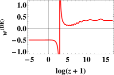
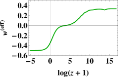
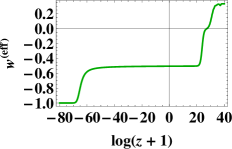
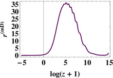
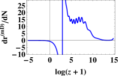
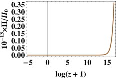
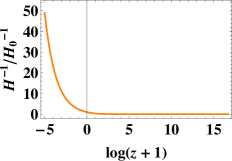
Figure 1: (color online). Cosmological solutions of $f(R,T)=R\log{(\alpha R)}+\sqrt{-T}$ gravity. The different cosmological parameters consist of the dark energy equation of state, the effective equation of state, $F(x_{2},x_{3})$, the ratio of the matter density to the dark energy density and its first derivative, and the Hubble parameter and its inverse. The initial values $x_{1}=10^{-7}$, $x_{2}=-10^{-6}$, $x_{3}=1.0058\times 10^{-6}$, $x_{4}=0.3\times 10^{-14}$, and $x_{5}=0.9999$ correspond to $z\thickapprox 1.78\times 10^{7}$. We used $\alpha=1.95\times 10^{92}$ in some plots. The diagrams are drawn to be consistent with the present value of $\Omega^{\textrm{(m)}}_{\textrm{0}}\approx 0.3$, $\Omega^{\textrm{(rad)}}_{\textrm{0}}\approx 10^{-4}$ and $H_{0}\simeq 67.3km/(Mpc.s)$. As it is obvious, the diagram for $F(x_{2},x_{3})$ has not a suitable range of value to indicate a matter–dominated era for which $F\approx 1$. The diagram of $r^{\textrm{(mD)}}$ shows that the value of $3/7$ appears twice in the evolution of the cosmos, and its ratio is about $-0.6$ at the present era. The matter dominates in the redshift $z\sim 33$, and from the diagram for $H^{-1}$, we find that in this epoch the relative size of the universe is about $9.4\times 10^{-3}$.

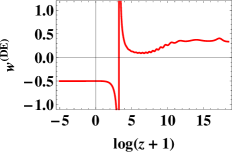
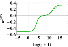
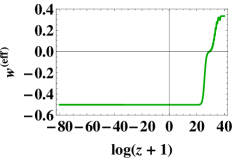
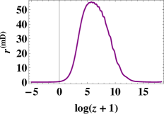
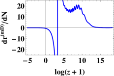
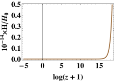
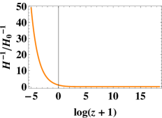
Figure 2: (color online). Cosmological solutions of $f(R,T)=R/\log{(\alpha R)}+\sqrt{-T}$ gravity. The initial values are $x_{1}=10^{-9}$, $x_{2}=-10^{-3}$, $x_{3}=1.006\times 10^{-3}$, $x_{4}=2.3\times 10^{-16}$ and $x_{5}=0.9999$ corresponding to $z\thickapprox 1.03\times 10^{8}$. We used $\alpha=5.7\times 10^{61}$ in some plots. The numerical data are matched to the present values of $\Omega^{\textrm{(m)}}_{\textrm{0}}\approx 0.3$, $\Omega^{\textrm{(rad)}}_{\textrm{0}}\approx 10^{-4}$ and $H_{0}\simeq 67.3km/(Mpc.s)$. In this case, the values of $F(x_{2},x_{3})$ are negative, which is not accepted. The matter–dominated era happens in the redshift $z\sim 60$, and the relative size of the universe in this era is about $4.1\times 10^{-3}$.

Table 2: Different features of $f(R,T)$ cosmological models.

$f(R,T)$ Model	$w^{\textrm{(DE)}}_{l}$	$H^{-1}_{0}$	$F^{\textrm{(m)}}$	$(\frac{dr}{dN}^{\textrm{(mD)}})_{0}$	$\alpha$	$z^{\textrm{(m)}}$	$q_{0}$	$j_{0}$	$s_{0}$
$R\log{(\alpha R)}+\sqrt{-T}$	$-1$	$9.3\times 10^{-3}$	138	-0.64	$1.95\times 10^{92}$	32.6	-0.027	0.21	-0.76
$R/\log{(\alpha R)}+\sqrt{-T}$	$-\frac{1}{2}$	$4.1\times 10^{-3}$	-0.005	-0.58	$5.7\times 10^{-61}$	58.7	-0.251	-0.12	0.18
$R+\alpha R^{1.01}+\sqrt{-T}$	$-\frac{1}{2}$	$5.9\times 10^{-3}$	1.66	-0.43	$1.371$	43.5	-0.016	0.23	-0.80
$R+\alpha R^{0.9}+\sqrt{-T}$	$-1$	$1.2\times 10^{-5}$	0.97	-0.68	$0.646\times 10^{-4}$	1104	-0.038	0.22	-0.76

III.2 $f(R,T)=R+\alpha R^{-n}+\sqrt{-T}$,   $n\neq 0$

In this case, from definitions (23) and (24), we have

$$m=-n\frac{x_{3}+x_{2}}{x_{3}},\leavevmode\nobreak\ \leavevmode\nobreak\ \leavevmode\nobreak\ \leavevmode\nobreak\ \leavevmode\nobreak\ \leavevmode\nobreak\ \leavevmode\nobreak\ \leavevmode\nobreak\ \leavevmode\nobreak\ \leavevmode\nobreak\ \leavevmode\nobreak\ \leavevmode\nobreak\ \leavevmode\nobreak\ \leavevmode\nobreak\ \leavevmode\nobreak\ \leavevmode\nobreak\ \leavevmode\nobreak\ \leavevmode\nobreak\ \leavevmode\nobreak\ \leavevmode\nobreak\ \leavevmode\nobreak\ \leavevmode\nobreak\ \leavevmode\nobreak\ \leavevmode\nobreak\ \leavevmode\nobreak\ \leavevmode\nobreak\ \frac{dm}{dN}=x_{1}(1-\frac{nx_{2}}{x_{3}}),$$ (69)

$$F(x_{2},x_{3})=(1+n)\frac{x_{3}}{x_{3}-nx_{2}}\leavevmode\nobreak\ \leavevmode\nobreak\ \leavevmode\nobreak\ \leavevmode\nobreak\ \leavevmode\nobreak\ \leavevmode\nobreak\ \leavevmode\nobreak\ \leavevmode\nobreak\ \leavevmode\nobreak\ \leavevmode\nobreak\ \mbox{and}\leavevmode\nobreak\ \leavevmode\nobreak\ \leavevmode\nobreak\ \leavevmode\nobreak\ \leavevmode\nobreak\ \leavevmode\nobreak\ \leavevmode\nobreak\ \leavevmode\nobreak\ \leavevmode\nobreak\ \leavevmode\nobreak\ H(x_{2},x_{3})=\sqrt{\frac{[\frac{x_{2}+x_{3}}{\alpha(nx_{2}-x_{3})}]^{\frac{-1}{1+n}}}{6x_{3}}},$$ (70)

where $r\neq n$. As we have indicated before, for $-\sqrt{|n|}<r_{i}<-1$ with $n\rightarrow-1^{-}$, the effective equation–of–state parameter has the value $-0.5$ (i.e., the related fixed point in the phase space is stable), and otherwise it gets $-1$. This means that it is important to choose an appropriate initial value for $r_{i}$ for consistency with the observations. Here, the behavior of the coincidence parameter, its derivative, and the dark energy equation–of–state parameter, for the model with $n=-1.01$, are shown in Figure 3. On the other hand, for the model with $n=-0.9$, we can set the initial values in a way that the pick of the matter density diagram occurs in the redshift about $z\simeq 1100$. The price for this consistency is that the matter–dominated era lasts for a long time. The relative size of the universe in this era is about $1.2\times 10^{-5}$, which is a more consistent value mukhanov . The related diagram for this model is drawn in Figure 4. It is obvious that $F(x_{2},x_{3})$ has approximately the value around one in the deep matter and radiation eras (i.e., $F\simeq 0.97$), which means $g(R)\thicksim R$ in such times. Again, the value $r^{\textrm{(mD)}}\simeq 3/7$ appears twice with $dr^{\textrm{(mD)}}/dN\simeq-0.6$. We have also plotted the related diagrams of the decelerated, the jerk, and the snap parameters in Figure 4. These diagrams show a consistence sequence for different cosmological eras, however, their present values $q_{0}\simeq-0.04$, $j_{0}\simeq 0.22$, and $s_{0}\simeq-0.76$ do not match the present observational data. The matter–dominated era for the theory with $n=-1.01$ occurs in the redshift $z\sim 43$ with the relative size of about $6\times 10^{-3}$. We have summarized the discussed features of these four models in Table 2, where the values of the deceleration, jerk, and snap parameters for the first three models are also presented.

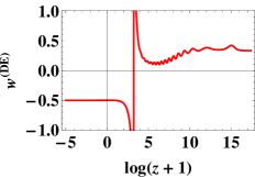
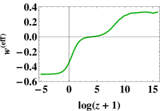
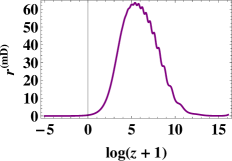
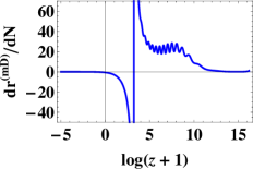
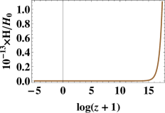
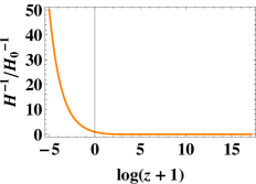
Figure 3: (color online). Cosmological solutions of $f(R,T)=R+\alpha R^{1.01}+\sqrt{-T}$ gravity. In this case, the initial values $x_{1}=10^{-8}$, $x_{2}=-10^{-5}$, $x_{3}=1.0049\times 10^{-5}$, $x_{4}=10^{-15}$, and $x_{5}=0.9999$ correspond to $z\thickapprox 3.6\times 10^{7}$. We have used $\alpha=1.43$ in some plots. In this theory, we reach at the same results as the previous two theories in subsection III.1, except the result of the function $F$, which is more reasonable in this theory. The matter–dominated era for the theory with $n=-1.01$ occurs in $z\sim 43$ with the relative size of the universe in this era about $6\times 10^{-3}$.

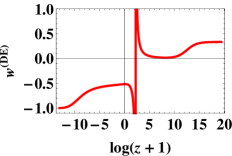
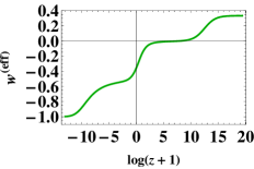
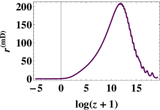
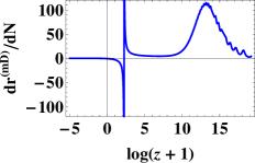
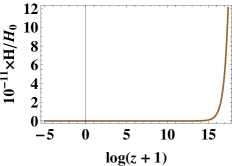
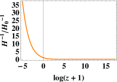
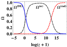
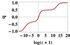
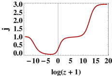
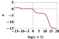
Figure 4: (color online). Cosmological solutions of $f(R,T)=R+\alpha R^{0.9}+\sqrt{-T}$ gravity. For this theory, we have chosen the initial values $x_{1}=10^{-6}$, $x_{2}=-10^{-3}$, $x_{3}=1.0001\times 10^{-3}$, $x_{4}=0.45\times 10^{-15}$, and $x_{5}=0.999$ that correspond to $z\thickapprox 2.6\times 10^{8}$ with $\alpha=4.06\times 10^{-5}$. The initial values are chosen in a way that the matter era occurs in the redshift of about $z_{m}\simeq 1100$, which corresponds to the last scattering surface. With these initial values, the radiation–matter equality takes place at $z\simeq 10^{5}$, which is far from the given results in the literature. Note that it is possible to choose some other initial values to solve this inconsistency, however, one should be careful about the other cosmological quantities, such as the value of the function $F$. The above diagrams for the deceleration, jerk, and snap parameters show a consistent sequence for different cosmological eras. However, their present values do not match the present observational data. For this theory, the relative size of the universe in this era is about $1.2\times 10^{-5}$.

IV Cosmological Solution of Model $f(R,T)=R+c_{1}\sqrt{-T}$

In this section, we investigate the cosmological properties of theory $f(R,T)=R+c_{1}\sqrt{-T}$. This theory is similar to theories with the dynamical cosmological constant. However, in contrast to the most of them, this theory does not include any scalar field as the matter field, which motivates one to extract the cosmological solutions of this theory. As in this case, we have $m(r)=0$, and the formalism presented in the first section does not work, hence, we should obtain the dynamical system equations independently. To complete the discussion, we include the spatial curvature term to investigate whether $f(R,T)$ gravity can select a particular sign for the curvature constant $k$. From equations (13) and (14) for $g(R)=R$, one obtains

$$1+c_{1}\frac{h}{6H^{2}}+\frac{k}{a^{2}H^{2}}=\frac{8\pi G\rho^{\textrm{(m)}}}{3H^{2}}+c_{1}\frac{h^{\prime}\rho^{\textrm{(m)}}}{3H^{2}}+\frac{8\pi G\rho^{\textrm{(rad)}}}{3H^{2}}$$ (71)

and

$$\frac{2\dot{H}}{H^{2}}-\frac{2k}{a^{2}H^{2}}=-\frac{8\pi G\rho^{\textrm{(m)}}}{H^{2}}-c_{1}\frac{h^{\prime}\rho^{\textrm{(m)}}}{H^{2}}-\frac{32\pi G\rho^{\textrm{(rad)}}}{3H^{2}},$$ (72)

where $k$ is normalized to $+1$, $0$, and $-1$ for a closed, flat, and open universe, respectively. Note that, the field equations (71) and (72) do not contain the variables $x_{1}$, $x_{2}$, and $x_{5}$, and therefore the only contained variables are $x_{3}$, $x_{4}$, $\Omega^{\textrm{(k)}}$, $\Omega^{\textrm{(rad)}}$, and $\Omega^{\textrm{(DE)}}$. Equation (71) gives

$$\Omega^{\textrm{(m)}}+\Omega^{\textrm{(k)}}+\Omega^{\textrm{(rad)}}+c_{1}\Omega^{\textrm{(DE)}}=1,$$ (73)

where from equation (39), and the definitions $x_{1}$ and $x_{2}$, in this case, we have $\Omega^{\textrm{(DE)}}=x_{4}$. Therefore, we incorporate four fluid densities, namely, the matter, spatial curvature, radiation, and dark energy ones.

On the other hand, by using equations (17) and (72), we reach at the following constraint

$$x_{3}=\frac{1}{2}-\frac{\Omega^{\textrm{(k)}}}{2}-\frac{\Omega^{\textrm{(rad)}}}{2}+\frac{3c_{1}\Omega^{\textrm{(DE)}}}{4}.$$ (74)

Thus, these two constraints, equations (73) and (74), eliminate the two variables $x_{3}$ and $\Omega^{\textrm{(m)}}$, and only three dimensionless density parameters, $\Omega^{\textrm{(k)}}$, $\Omega^{\textrm{(rad)}}$, and $\Omega^{\textrm{(DE)}}$, remain as the independent variables. For the effective equation–of–state parameter, we obtain

$$w^{\textrm{(eff)}}=\frac{1}{3}\left(\Omega^{\textrm{(rad)}}-\Omega^{\textrm{(k)}}\right)-c_{1}\frac{\Omega^{\textrm{(DE)}}}{2}.$$ (75)

Hence, we have a three–variable phase space with the following equations of motion

$$\frac{d\Omega^{\textrm{(k)}}}{dN}=\Omega^{\textrm{(k)}}\left(1+\Omega^{\textrm{(rad)}}-\Omega^{\textrm{(k)}}-c_{1}\frac{3\Omega^{\textrm{(DE)}}}{2}\right),$$ (76)

$$\frac{d\Omega^{\textrm{(rad)}}}{dN}=\Omega^{\textrm{(rad)}}\left(-1+\Omega^{\textrm{(rad)}}-\Omega^{\textrm{(k)}}-c_{1}\frac{3\Omega^{\textrm{(DE)}}}{2}\right),$$ (77)

$$\frac{d\Omega^{\textrm{(DE)}}}{dN}=\Omega^{\textrm{(DE)}}\left(\frac{3}{2}+\Omega^{\textrm{(rad)}}-\Omega^{\textrm{(k)}}-c_{1}\frac{3\Omega^{\textrm{(DE)}}}{2}\right).$$ (78)

In Table 3, we have shown the fixed points and their stability properties. There are four fixed points comprised of the point $P^{\textrm{(DE)}}$ that determines an acceleration–expansion–dominated era, the point $P^{\textrm{(k)}}$ that refers to an era in which the spatial curvature density is dominated over the other densities, the point $P^{\textrm{(rad)}}$ that indicates a radiation–dominated era, and, finally, the point $P^{\textrm{(m)}}$ that points to a matter–dominated era. It is clear that only the dark energy fixed point is stable, for the appearance of negative eigenvalues. It means that the dark–energy–dominated era is an everlasting era. Nevertheless, this fixed point corresponds to $w^{\textrm{(eff)}}=-1/2$, which is not an observational consistent value. The saddle fixed point $P^{\textrm{(k)}}$ indicates $\Omega^{\textrm{(k)}}=1$, which refers to an open universe. There is no solution with $\Omega^{\textrm{(k)}}=-1$ as a closed universe.

Table 3: The fixed points solutions of $f(R,T)=R+c_{1}\sqrt{-T}$ gravity radiation.

Fixed point	Coordinates $(\Omega^{\textrm{(k)}},\Omega^{\textrm{(rad)}},\Omega^{\textrm{(DE)}})$	Eigenvalues	$\Omega^{\textrm{(m)}}$	$w^{\textrm{(eff)}}$
$P^{\textrm{(DE)}}$	$(0,0,\frac{1}{c_{1}})$	$(-\frac{5}{2},-\frac{3}{2},-\frac{1}{2})$	$0$	$-\frac{1}{2}$
$P^{\textrm{(k)}}$	$(1,0,0)$	$(-2,-1,\frac{1}{2})$	$0$	$-\frac{1}{3}$
$P^{\textrm{(rad)}}$	$(0,1,0)$	$(5,2,1)$	$0$	$\frac{1}{3}$
$P^{\textrm{(m)}}$	$(0,0,0)$	$(\frac{3}{2},-1,1)$	$1$	$0$

As Table 3 shows, the dark energy density parameter depends on the coupling constant $c_{1}$, and hence it is constrained to have positive values. However, it does not affect the stability properties of the fixed points and the value of the equation–of–state parameter. In Figure 5, we have depicted the density parameters for an open universe. These diagrams show that for large values of $c_{1}$ the dark energy density parameter tends to small values, which means that the late–time era is effectively dominated by dust–like matter. In such situations, the magnitude of the spatial curvature density decreases to smaller values. On the other hand, for $0<c_{1}<1$, the pressureless matter density gets negative values, which is not physically justified. Also in these cases, the magnitude of the spatial curvature density increases to larger values. We have checked that the results for a closed universe are the same as the ones for an open universe. Nevertheless, to have a dominant dark energy era with $\Omega^{\textrm{(DE)}}\simeq 1$, the preferred value for the coupling constant is $c_{1}\simeq 1$ (in our assumed units), and we will adopt this value in the rest of this work. Thus, the terms $R$ and $\sqrt{-T}$ are placed of the same order of magnitude in the Lagrangian (again in our assumed units). Also, we have checked that the minimal models $f(R,T)=g(R)+h(T)$, discussed in Sec. II, show similar behaviors.

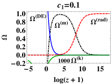
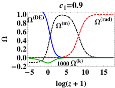
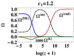
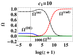
Figure 5: (color online). The effects of coupling constant $c_{1}$ on the fluid density parameters in $f(R,T)=R+c_{1}\sqrt{-T}$ gravity for an open universe. The radiation density parameter is not affected by this constant. The larger (smaller) values of $c_{1}$ leads to small (larger) values of the dark energy and the spatial curvature densities.

We have drawn the diagrams for the density components and the dark energy equation of state for the both positive and negative initial values of $\Omega^{\textrm{(k)}}$ in Figure 6. As is obvious, for the both initial values, the amplitude of $\Omega^{\textrm{(k)}}$ is not far from the observational data, i.e., the diagrams also indicate that for an open universe we have $\Omega^{\textrm{(k)}}\simeq 10^{-3}$ and for a closed one $\Omega^{\textrm{(k)}}\simeq 10^{-4}$. In Figure 6, the diagrams show that $\Omega^{\textrm{(k)}}$, in the matter–dominated era, is small and the curvature domination occurs in the late times and large scales. The other diagrams illustrate the evolution of the equation–of–state parameter for the dark energy, both in an open and a closed universe. For an open (closed) universe, the corresponding curve has an increasing (decreasing) feature to the value $w^{\textrm{(eff)}}=-1/2$. This contrast gives us an opportunity to match it with the observations. Irrespective of the non–consistent value $w^{\textrm{(eff)}}=-1/2$, the increasing (decreasing) feature can be a distinguishable criteria. If the evolution of $w^{\textrm{(eff)}}$ in different cosmological eras can be investigated from the observational data, then the increasing (decreasing) feature will rule out any inconsistent cosmological model.

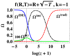
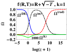
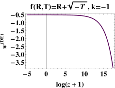
Figure 6: (color online). Cosmological solutions of $f(R,T)=R+c_{1}\sqrt{-T}$ gravity with $c_{1}=1$. These diagrams accept the initial values $\Omega^{\textrm{(rad)}}=0.9999$, $\Omega^{\textrm{(DE)}}=10^{-15}$, and $\Omega^{\textrm{(k)}}=10^{-15}$ for an open universe and the same values, but with $\Omega^{\textrm{(k)}}=-10^{-15}$, for a closed universe, corresponding to $z\thickapprox 3.6\times 10^{7}$. The diagrams show $\Omega^{\textrm{(k)}}_{0}=10^{-3}$ for the open universe and $\Omega^{\textrm{(k)}}_{0}=-10^{-4}$ for the closed universe. The dark energy curve has an increasing behavior up to the value $w^{\textrm{(eff)}}=-1/2$ for the open universe, and it has a decreasing behavior down to the value $w^{\textrm{(eff)}}=-1/2$ for the closed universe.

In Figure 7, we have presented a parametric plot in $(\Omega^{\textrm{(k)}},\Omega^{\textrm{(rad)}},\Omega^{\textrm{(DE)}})$ coordinates for the left diagram and in $(\Omega^{\textrm{(k)}},\Omega^{\textrm{(rad)}},\Omega^{\textrm{(m)}})$ coordinates for the right one, both in an open universe. Both diagrams show an acceptable evolution of the density parameters. The left figure illustrates that $\Omega^{\textrm{(k)}}$ has a peak when $\Omega^{\textrm{(DE)}}\simeq 0.7$, and the right figure indicates that it happens when $\Omega^{\textrm{(m)}}\simeq 0.3$.

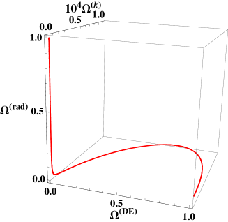
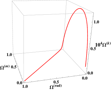
Figure 7: (color online). Cosmological solutions of $f(R,T)=R+c_{1}\sqrt{-T}$ gravity for $k=-1$. The left parametric plot is in terms of $\Omega^{\textrm{(k)}}$, $\Omega^{\textrm{(rad)}}$, and $\Omega^{\textrm{(DE)}}$, and the right one is in terms of $\Omega^{\textrm{(k)}}$, $\Omega^{\textrm{(rad)}}$, and $\Omega^{\textrm{(m)}}$ coordinates. The peaks of the curves occur at $\Omega^{\textrm{(DE)}}\simeq 0.7$ in the left and at $\Omega^{\textrm{(m)}}\simeq 0.3$ in the right diagrams, respectively.

Also, in Figure 8, we have depicted a phase portrait of the solutions in the surface $\Omega^{\textrm{(k)}}=0$. In this plot, for some initial values, we have a few trajectories that, after leaving the radiation fixed point, approach the matter fixed point and finally are attracted to the dark energy fixed point. Among the trajectories, there are ones that directly connect the early era (corresponding to the radiation fixed point) to the late–time era (corresponding to the dark energy fixed point) without passing the matter era (corresponding to the matter fixed point). Some trajectories connect the matter era to the accelerated expansion era without starting from the radiation era, etc. Note that the negative valued regions are not related to our solutions.

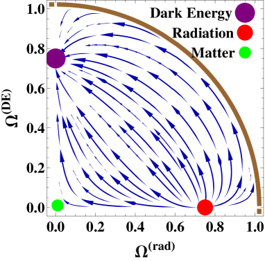
Figure 8: (color online). A phase portrait for the special case $k=0$ is drawn. There is an acceptable trajectory that connects the radiation era to the matter era then to the dark–energy–dominated era as the final attractor. The other trajectories do not contain any proper cosmological sequence.

V Weak–field limit of $f(R,T)$ gravity models

In this section, we consider the weak–field limit of $f(R,T)$ gravity. To perform this task, we implicitly assume those models that admit Taylor series expansion around the background values of the Ricci scalar and the trace of the energy–momentum tensor. In addition, we work on a pressureless matter, where in this case, the magnitude of the trace is the same as the mass density of matter. To consider the weak–field limit of $f(R,T)$ gravity, we first linearize the field equation (3) (which we preferably rewrite as

$$F(R,T)R_{\mu\nu}-\frac{1}{2}f(R,T)g_{\mu\nu}+\Big{(}g_{\mu\nu}\square-\triangledown_{\mu}\triangledown_{\nu}\Big{)}F(R,T)=\Big{(}8\pi G+{\mathcal{F}}(R,T)\Big{)}T_{\mu\nu},$$ (79)

where $T_{\mu\nu}$ generally depends on the spatial coordinates and time). In comparison, in $f(R)$ gravity, only the matter density perturbation sources the perturbation of the Ricci scalar, but in $f(R,T)$ gravity, the perturbation of the trace of the energy–momentum tensor also sources the perturbation of the curvature of space–time. Here, we investigate the space–time metric outside a spherical body and then determine the PPN gamma parameter to confront the $f(R,T)$ models with the observational data. We should remind the reader that, in the literature, the PPN parameter of $f(R)$ gravity, without resorting to the scalar–tensor equivalence, has been obtained to be $\gamma^{\textrm{(f(R))}}=1/2$ solar1 , nevertheless, in this theory, using a scalar–tensor representation, one can still acquire an observational consistent value, which is supposed to be $\gamma^{\textrm{(obs)}}=1+(2.1\pm 2.3)\times 10^{-5}$ ppn1 ; ppn2 .

Now, we suppose a background space–time that is usually assumed to be the isotropic and homogeneous one. This space–time admits a background spatially uniform energy–momentum tensor $T_{\mu\nu}^{\textrm{(b)}}$. For the background space–time with a background energy–momentum tensor $T_{\mu\nu}^{\textrm{(b)}}$, we have

$$F^{\textrm{(b)}}(t)R_{\mu\nu}^{\textrm{(b)}}(t)-\frac{1}{2}f^{\textrm{(b)}}(t)g_{\mu\nu}^{\textrm{(b)}}(t)+\Big{(}g_{\mu\nu}^{\textrm{(b)}}(t)\square-\triangledown_{\mu}\triangledown_{\nu}\Big{)}F^{\textrm{(b)}}(t)=\Big{(}8\pi G+\mathcal{F}^{\textrm{(b)}}(t)\Big{)}T^{\textrm{(b)}}_{\mu\nu}(t),$$ (80)

where $F^{\textrm{(b)}}\equiv\partial f/\partial R|_{(R^{\textrm{(b)}},T^{\textrm{(b)}})}$, $f^{\textrm{(b)}}\equiv f(R^{\textrm{(b)}},T^{\textrm{(b)}})$, and $\mathcal{F}^{\textrm{(b)}}\equiv\partial f/\partial T|_{(R^{\textrm{(b)}},T^{\textrm{(b)}})}$. The supper script $b$ denotes the background quantities, and we have dropped the argument $(R,T)$. By the argument $t$, we have indicated that all the background quantities depend only on the cosmic time. Using the trace of equation (79), one can determine the evolution of time–dependent scalar curvature $R^{\textrm{(b)}}(t)$ as

$$F^{\textrm{(b)}}(t)R^{\textrm{(b)}}(t)+3\Box F^{\textrm{(b)}}(t)-2f^{\textrm{(b)}}(t)=(8\pi G+\mathcal{F}^{\textrm{(b)}}(t))T^{\textrm{(b)}}(t).$$ (81)

To linearize the field equation (79) and its trace equation, we perturb the Ricci scalar, the Ricci tensor, the energy–momentum tensor and its trace as the sum of a time–dependent spatially homogeneous background component and a time–independent source component, namely

$$R(t,r)=R^{\textrm{(b)}}(t)+R^{\textrm{(s)}}(r),$$ (82)

$$R_{\mu\nu}(t,r)=R^{\textrm{(b)}}_{\mu\nu}(t)+R^{\textrm{(s)}}_{\mu\nu}(r),$$ (83)

$$T_{\mu\nu}(t,r)=T_{\mu\nu}^{\textrm{(b)}}(t)+T_{\mu\nu}^{\textrm{(s)}}(r),$$ (84)

$$T(t,r)=T^{\textrm{(b)}}(t)+T^{\textrm{(s)}}(r).$$ (85)

The background metric is taken to be the FLRW metric (9) with $k=0$, and its spherically symmetric linearized form reads

$$ds^{2}=-\Big{(}1+2\Psi(r)\Big{)}dt^{2}+a^{2}(t)\left[\Big{(}1+2\Phi(r)\Big{)}dr^{2}+r^{2}d\Omega^{2}\right],$$ (86)

where $\Psi(r)$ and $\Phi(r)$ are the metric perturbations. To proceed, we use the Taylor expansion of the functions $f(R,T)$, $F(R,T)$, and $\mathcal{F}(R,T)$ around the background quantities $R^{\textrm{(b)}}$ and $T^{\textrm{(b)}}$. Further, we neglect the non–linear terms in the expansions, assuming that the zeroth and the first terms dominate these terms. Therefore, the first–order version of the trace of equation (79) is obtained as

$$\nabla^{2}R^{\textrm{(s)}}-m^{2}_{\textrm{f(R,T)}}R^{\textrm{(s)}}=\mathcal{S},$$ (87)

where we have defined a mass parameter

$$m^{2}_{\textrm{f(R,T)}}\equiv\frac{1}{3}\left(\frac{F^{\textrm{(b)}}}{F_{R}^{\textrm{(b)}}}+\frac{\mathcal{F}_{\textrm{R}}^{\textrm{(b)}}}{F_{\textrm{R}}^{\textrm{(b)}}}T^{\textrm{(b)}}-R^{\textrm{(b)}}+\frac{3}{F_{\textrm{R}}^{\textrm{(b)}}}\frac{d^{2}F_{\textrm{R}}^{\textrm{(b)}}}{dt^{2}}\right),$$ (88)

a source parameter

$$\mathcal{S}\equiv\frac{1}{3F_{\textrm{R}}^{\textrm{(b)}}}\left[\left(8\pi G+3\mathcal{F}^{\textrm{(b)}}+\mathcal{F}_{\textrm{T}}^{\textrm{(b)}}T^{\textrm{(b)}}-F_{\textrm{T}}^{\textrm{(b)}}R^{\textrm{(b)}}-3\frac{d^{2}F_{\textrm{T}}^{\textrm{(b)}}}{dt^{2}}\right)T^{\textrm{(s)}}-3F_{\textrm{T}}^{\textrm{(b)}}\nabla^{2}T^{\textrm{(s)}}\right]$$ (89)

and we have used $\Box\,\Xi^{\textrm{(b)}}(t)=-d^{2}\Xi^{\textrm{(b)}}(t)/dt^{2}$ and $\Box\,\Xi^{\textrm{(s)}}(r)=\nabla^{2}\Xi^{\textrm{(s)}}(r)$ for any arbitrary function $\Xi$. Also, we have defined $F_{\textrm{R}}\equiv\partial F/\partial R$, $F_{\textrm{T}}\equiv\partial F/\partial T$, $\mathcal{F}_{\textrm{R}}\equiv\partial\mathcal{F}/\partial R$, and $\mathcal{F}_{\textrm{T}}\equiv\partial\mathcal{F}/\partial T$, and in obtaining equation (87), we have neglected all the second–order terms like $F_{\textrm{T}}^{\textrm{(b)}}T^{\textrm{(s)}}R^{\textrm{(s)}}$. It is obvious that the mass parameter (88) varies in time, however, its variation is negligible with respect to the cosmological time–scale variations that are of the order of the current Hubble time. Hence, we take $m^{2}_{\textrm{f(R,T)}}$ to be a time–independent parameter. Since, the time scale of the solar system experiments is negligible compared to the cosmological time scale, one can discard the time derivative of all the quantities and therefore can use the present value of the background quantities for the solar system applications. On the other hand, $H^{2}$ is of the order of the inverse squared age of the universe, and hence it is negligible at the present era, similarly for the quantities $R^{\textrm{(b)}}\sim H^{2}$, $d^{2}\ln{(F_{\textrm{R}}^{\textrm{(b)}})}/dt^{2}\sim H^{2}$ solar1 . We also set the present value of the scale factor as $1$. Therefore, the mass parameter (88) and the source expression (89) can be written as

$$m^{2}_{\textrm{f(R,T)}}\simeq\frac{1}{3}\left(\frac{F^{\textrm{(b)}}}{F_{\textrm{R}}^{\textrm{(b)}}}+\frac{\mathcal{F}_{\textrm{R}}^{\textrm{(b)}}}{F_{\textrm{R}}^{\textrm{(b)}}}T^{\textrm{(b)}}\right)$$ (90)

and

$$\mathcal{S}\simeq\frac{1}{3F_{\textrm{R}}^{\textrm{(b)}}}\left[\left(8\pi G+3\mathcal{F}^{\textrm{(b)}}+\mathcal{F}_{\textrm{T}}^{\textrm{(b)}}T^{\textrm{(b)}}\right)T^{\textrm{(s)}}-3F_{\textrm{T}}^{\textrm{(b)}}\nabla^{2}T^{\textrm{(s)}}\right].$$ (91)

The study of the Green functions for equation (87) shows that in the limit $|m^{2}_{\textrm{f(R,T)}}|r^{2}\ll 1$, these functions approximately take the form $-1/(4\pi r)$, which is the Green function for the Laplace equation solar1 . Hence, in this limit, the second term in equation (87) may be neglected, and then the corresponding differential equation for $R^{\textrm{(s)}}$ takes the following form

$$\nabla^{2}R^{\textrm{(s)}}\simeq\mathcal{S}.$$ (92)

In this case, the exterior solution of equation (92) for a spherical body with mass $M$, radius $\Re$, and mass density $\rho^{\textrm{(s)}}(r)$ can be obtained as

$$R^{\textrm{(s)}}\simeq\frac{2G^{\textrm{(eff)}}M}{3F_{\textrm{R}}^{\textrm{(b)}}r}+\frac{F_{\textrm{T}}^{\textrm{(b)}}\mathcal{M}^{\textrm{(sur)}}(\Re)}{F_{\textrm{R}}^{\textrm{(b)}}r},$$ (93)

where we have assumed that all the perturbations vanish at long distances. In solution (93), we have defined a quantity that has the dimension of mass per area of body surface, i.e.,

$$\mathcal{M}^{\textrm{(sur)}}(r)\equiv 4\pi r^{2}\frac{d\rho^{\textrm{(s)}}(r)}{dr}.$$ (94)

This term comes from $\nabla^{2}T^{\textrm{(s)}}$, which is a new one in $f(R,T)$ gravity with respect to the $f(R)$ gravity worked in Ref. solar1 . Also, in solution (93), we have defined an effective gravitational constant $G^{\textrm{(eff)}}$ as

$$G^{\textrm{(eff)}}\equiv G+\frac{1}{8\pi}\left[3\mathcal{F}^{\textrm{(b)}}+\mathcal{F}_{\textrm{T}}^{\textrm{(b)}}T^{\textrm{(b)}}\right].$$ (95)

Note that the condition $|m^{2}_{\textrm{f(R,T)}}|r^{2}\ll 1$ leads to

$$\left|\frac{F^{\textrm{(b)}}}{F_{\textrm{R}}^{\textrm{(b)}}}+\frac{\mathcal{F}_{\textrm{R}}^{\textrm{(b)}}}{F_{\textrm{R}}^{\textrm{(b)}}}T^{\textrm{(b)}}\right|r^{2}=\left|\frac{F^{\textrm{(b)}}}{F_{\textrm{R}}^{\textrm{(b)}}}\left(1+\frac{\mathcal{F}_{\textrm{R}}^{\textrm{(b)}}}{F^{\textrm{(b)}}}T^{\textrm{(b)}}\right)\right|r^{2},$$ (96)

where, provided that $|(\mathcal{F}_{\textrm{R}}^{\textrm{(b)}}/F^{\textrm{(b)}})T^{\textrm{(b)}}|\ll 1$, the corresponding condition for $f(R)$ gravity solar1 is recovered, i.e.,

$$\left|\frac{F^{\textrm{(b)}}}{F_{\textrm{R}}^{\textrm{(b)}}}\right|r^{2}\ll 1.$$ (97)

Now, let us obtain the metric perturbations $\Psi(r)$ and $\Phi(r)$ by using solution (93). For this purpose, the first–order Taylor expansion of the field equation (79) yields

$$F^{\textrm{(b)}}R^{\textrm{(s)}\nu}_{\mu}+\left(F_{\textrm{R}}^{\textrm{(b)}}R^{\textrm{(b)}\nu}_{\mu}-\frac{1}{2}\delta^{\nu}_{\mu}F^{\textrm{(b)}}+\delta^{\nu}_{\mu}F_{\textrm{R}}^{\textrm{(b)}}\Box-F_{\textrm{R}}^{\textrm{(b)}}\nabla_{\mu}\nabla^{\nu}-\mathcal{F}_{\textrm{R}}^{\textrm{(b)}}T^{\textrm{(b)}\nu}_{\mu}+\delta^{\nu}_{\mu}\Box F_{\textrm{R}}^{\textrm{(b)}}-\nabla_{\mu}\nabla^{\nu}F_{\textrm{R}}^{\textrm{(b)}}\right)R^{\textrm{(s)}}=$$

$$\left(8\pi G+\mathcal{F}^{\textrm{(b)}}\right)T^{\textrm{(s)}\nu}_{\mu}+\left(\mathcal{F}_{\textrm{T}}^{\textrm{(b)}}T^{\textrm{(b)}\nu}_{\mu}-F_{\textrm{T}}^{\textrm{(b)}}R^{\textrm{(b)}\nu}_{\mu}+\frac{1}{2}\delta^{\nu}_{\mu}\mathcal{F}^{\textrm{(b)}}-\delta^{\nu}_{\mu}F_{\textrm{T}}^{\textrm{(b)}}\Box+F_{\textrm{T}}^{\textrm{(b)}}\nabla_{\mu}\nabla^{\nu}-\delta^{\nu}_{\mu}\Box F_{\textrm{T}}^{\textrm{(b)}}+\nabla_{\mu}\nabla^{\nu}F_{\textrm{T}}^{\textrm{(b)}}\right)T^{\textrm{(s)}},$$ (98)

of which the $tt$, $rr$, and $\theta\theta$ equations, for a pressureless fluid, are approximated to give

$$F^{\textrm{(b)}}\nabla^{2}\Psi+\left(\frac{1}{2}F^{\textrm{(b)}}-\mathcal{F}_{\textrm{R}}^{\textrm{(b)}}\rho^{\textrm{(b)}}\right)R^{\textrm{(s)}}-F_{\textrm{R}}^{\textrm{(b)}}\nabla^{2}R^{\textrm{(s)}}=\left(8\pi G^{\textrm{(eff)}}-\frac{3}{2}\mathcal{F}^{\textrm{(b)}}+F_{\textrm{T}}^{\textrm{(b)}}\nabla^{2}\right)\rho^{\textrm{(s)}},$$ (99)

$$F^{\textrm{(b)}}(-\Psi^{\prime\prime}+\frac{2}{r}\Phi^{\prime})-\frac{1}{2}F^{\textrm{(b)}}R^{\textrm{(s)}}+\frac{2}{r}F_{\textrm{R}}^{\textrm{(b)}}R^{\prime\textrm{(s)}}=-\frac{1}{2}\mathcal{F}^{\textrm{(b)}}\rho^{\textrm{(s)}}+\frac{2}{r}F_{\textrm{T}}^{\textrm{(b)}}\rho^{\prime\textrm{(s)}},$$ (100)

$$F^{\textrm{(b)}}(\frac{1}{r}\Phi^{\prime}-\frac{1}{r}\Psi^{\prime}+\frac{2}{r^{2}}\Phi)-\frac{1}{2}F^{\textrm{(b)}}R^{\textrm{(s)}}+\frac{1}{r}F_{\textrm{R}}^{\textrm{(b)}}R^{\prime\textrm{(s)}}+F_{\textrm{R}}^{\textrm{(b)}}R^{\prime\prime\textrm{(s)}}=-\frac{1}{2}\mathcal{F}^{\textrm{(b)}}\rho^{\textrm{(s)}}+\frac{1}{r}F_{\textrm{T}}^{\textrm{(b)}}\rho^{\prime\textrm{(s)}}+F_{\textrm{T}}^{\textrm{(b)}}\rho^{\prime\prime\textrm{(s)}},$$ (101)

where the prime indicates differentiation with respect to $r$. By considering solution (93), one does expect that $\Psi(r)$ and $\Phi(r)$ will have similar functionality to $r$, which implies that the terms $R^{\textrm{(s)}}\Psi$ and $R^{\textrm{(s)}}\Phi$ are of second–order, and hence we have neglected them in obtaining the filed equations (99)– (101). Therefore, the most general form of the potential $\Psi(r)$, outside the body, using (92), (93), and (99), can be obtained as

$$\Psi(r)=-\frac{4G^{\textrm{(eff)}}M}{3F^{\textrm{(b)}}r}+\frac{3\mathcal{F}^{\textrm{(b)}}M}{8\pi F^{\textrm{(b)}}r}-\left(\frac{G^{\textrm{(eff)}}M}{3F_{\textrm{R}}^{\textrm{(b)}}}+\frac{F_{\textrm{T}}^{\textrm{(b)}}\mathcal{M}^{\textrm{(sur)}}(\Re)}{2F_{\textrm{R}}^{\textrm{(b)}}}\right)\left(\frac{1}{2}-\frac{\mathcal{F}_{\textrm{R}}^{\textrm{(b)}}T^{\textrm{(b)}}}{F^{\textrm{(b)}}}\right)r-\frac{C_{1\Psi}}{r}+C_{2\Psi},$$ (102)

where $C_{1\Psi}$ and $C_{2\Psi}$ are the integral constants and we have assumed $F^{\textrm{(b)}}\neq 0$. One can set $C_{2\Psi}=0$ as usually done in the Newtonian limit. In addition, the term containing $C_{1\Psi}$ leads to singularity in the origin, and hence one can discard it solar1 ; solar2 ; solar3 . Also, for the cases in which the condition $|(\mathcal{F}_{\textrm{R}}^{\textrm{(b)}}/F^{\textrm{(b)}})T^{\textrm{(b)}}|\ll 1$ holds, we rewrite $\Psi(r)$ as

$$\Psi(r)\simeq-\frac{4G^{\textrm{(eff)}}M}{3F^{\textrm{(b)}}r}+\frac{3\mathcal{F}^{\textrm{(b)}}M}{8\pi F^{\textrm{(b)}}r}-\frac{G^{\textrm{(eff)}}M}{6F_{\textrm{R}}^{\textrm{(b)}}}r+\frac{F_{\textrm{T}}^{\textrm{(b)}}\mathcal{M}^{\textrm{(sur)}}(\Re)}{4F_{\textrm{R}}^{\textrm{(b)}}}r.$$ (103)

We can further simplify solution (103) by comparing the third and fourth terms with respect to the first term, i.e.,

$$\left|\frac{G^{\textrm{(eff)}}Mr/6F_{\textrm{R}}^{\textrm{(b)}}}{4G^{\textrm{(eff)}}M/3F^{\textrm{(b)}}r}\right|=\left|\frac{F^{\textrm{(b)}}}{8F_{\textrm{R}}^{\textrm{(b)}}}\right|r^{2}\ll 1$$ (104)

and

$$\left|\frac{F_{\textrm{T}}^{\textrm{(b)}}\mathcal{M}^{\textrm{(sur)}}(\Re)r/4F_{\textrm{R}}^{\textrm{(b)}}}{4G^{\textrm{(eff)}}M/3F^{\textrm{(b)}}r}\right|=\left|\mathcal{B}\frac{F^{\textrm{(b)}}}{F_{\textrm{R}}^{\textrm{(b)}}}\right|r^{2},$$ (105)

where we have defined

$$\mathcal{B}\equiv\frac{\mathcal{M}^{\textrm{(sur)}}(\Re)}{M}\frac{3F_{\textrm{T}}^{\textrm{(b)}}}{16G^{\textrm{(eff)}}}.$$ (106)

In definition (106), the value of the first fraction is of the order of the magnitude of a surface mass per the total mass of the body which is usually less than $1$. Thus, if $3F_{\textrm{T}}^{\textrm{(b)}}/16G^{\textrm{(eff)}}$ does not get infinite or large values, one can neglect the fourth term in solution (103). Note that the fourth term in solution (103) already vanishes for minimal models, for which $F_{\textrm{T}}=0$. Finally, the form of the potential $\Psi$ reads

$$\Psi(r)\simeq-\frac{4G^{\textrm{(eff)}}M}{3F^{\textrm{(b)}}r}+\frac{3\mathcal{F}^{\textrm{(b)}}M}{8\pi F^{\textrm{(b)}}r}=-\left[\frac{4}{3}G+\frac{1}{8\pi}\left(\mathcal{F}^{\textrm{(b)}}+4\mathcal{F}_{\textrm{T}}^{\textrm{(b)}}T^{\textrm{(b)}}\right)\right]\frac{M}{F^{\textrm{(b)}}r}.$$ (107)

Comparing $\Psi(r)$ with the Newtonian potential, $-G^{(\textrm{N})}M/r$, gives

$$G=\frac{3}{4}F^{\textrm{(b)}}G^{\textrm{(N)}}-\frac{1}{8\pi}\left(\frac{3}{4}\mathcal{F}^{\textrm{(b)}}+\mathcal{F}_{\textrm{T}}^{\textrm{(b)}}T^{\textrm{(b)}}\right),$$ (108)

which shows that the deviation from the corresponding result of $f(R)$ gravity solar1 is the appearance of the second and third terms that depend on the background matter density. Nevertheless, the appearance of the trace–dependent terms is not a new result. Actually, it is reminiscent of the Palatini formulation of $f(R)$ gravity theories, wherein the trace of the corresponding field equations reads olmo

$$RF(R)-2f(R)=8\pi GT,$$

where $R$ is the metric–independent Ricci scalar. This equation for a well–defined function of $f(R)$ provides an algebraic equation for the Ricci scalar, and therefore, one can conclude that $R=R(T)$ and $F=F(T)$. This dependence has some interesting results in the solar system applications. In the weak–field limit of the Palatini formulation of these theories, for a pressureless fluid, one obtains olmo

$$g_{tt}=-\frac{1}{\varphi(T)}\left(1-\frac{2GM(r)}{r}\right)e^{2(\psi(r)-\psi_{0})},$$

where $M(r)$ and $\psi(r)$ are some functions of the radius $r$, $\psi_{0}$ is a constant and $\varphi(T)\equiv F(0)/F(T)$. As is obvious, $g_{tt}$ has been modified by a trace–dependent coefficient as our result(107).

In our case, the potential $\Phi(r)$ is also attained from equation (100), by using solutions (93) and (107) outside the spherical body, i.e.,

$$\Phi(r)\simeq\frac{2G^{\textrm{(eff)}}M}{3F^{\textrm{(b)}}r}-\frac{3\mathcal{F}^{\textrm{(b)}}M}{8\pi F^{\textrm{(b)}}r}=\left[\frac{2}{3}G+\frac{1}{8\pi}\left(-\mathcal{F}^{\textrm{(b)}}+\frac{2}{3}\mathcal{F}_{\textrm{T}}^{\textrm{(b)}}T^{\textrm{(b)}}\right)\right]\frac{M}{F^{\textrm{(b)}}r}.$$ (109)

One can easily check that solutions (107) and (109) satisfy equation (101) outside the body. Hence, in $f(R,T)$ gravity, the PPN gamma parameter, which is related to the potential $\Phi$ via $\Phi=\gamma G^{\textrm{(N)}}M/r$ will , is obtained to be

$$\gamma^{(\textrm{f(R,T)})}=\frac{1}{2}-\frac{3\mathcal{F}^{\textrm{(b)}}}{16\pi G^{\textrm{(N)}}F^{\textrm{(b)}}}.$$ (110)

That is, in $f(R,T)$ gravity, we generally have a running PPN parameter that depends on both the background matter density and the Ricci scalar . Thus, $f(R,T)$ gravity may has some chances to be made consistent with the solar system experiments by constructing some plausible models.

In equation (110), by setting $\mathcal{F}^{\textrm{(b)}}=0$, one recovers the corresponding result obtained for $f(R)$ gravity as in Ref. solar1 . However, in the literature olmo1 ; olmo2 , it has been indicated that applying a scalar–tensor representation for $f(R)$ gravity leads to a significant effect in its corresponding PPN parameter. Actually, the corresponding result $\gamma^{(\textrm{f(R)})}=1/2$ of Ref. solar1 is valid when the condition $|m_{\textrm{f(R)}}^{2}|r^{2}\ll 1$ is held. This condition, in a scalar–tensor representation of $f(R)$ gravity, denotes a light scalar field (i.e., $|m^{2}_{\textrm{f(R)}}|\ll 1$) with long interaction ranges. On the other hand, one can obtain $\gamma^{(\textrm{f(R)})}\simeq 1$ by setting the condition $|m_{\textrm{f(R)}}^{2}|r^{2}\gg 1$, which is translated to as the appearance of a heavy scalar field (i.e., $|m^{2}_{\textrm{f(R)}}|\gg 1$) with short interaction ranges. Therefore, depending on the mass of the scalar degree of freedom related to the curvature (which is model–dependent), one can get the desired result for this parameter, that is, the PPN parameter in $f(R)$ gravity is not also constrained to the value $1/2$.

In the following, we consider the $\gamma^{(\textrm{f(R,T)})}$ parameter for general minimal power law $f(R,T)$ models.

$\mathbf{General\leavevmode\nobreak\ Minimal\leavevmode\nobreak\ Power\leavevmode\nobreak\ Law\leavevmode\nobreak\ Case}\leavevmode\nobreak\ f(R,T)=c_{\textrm{R}}R^{n}+c_{\textrm{T}}T^{m}$

These models have

$$F=nc_{\textrm{R}}R^{n-1},\leavevmode\nobreak\ \leavevmode\nobreak\ \leavevmode\nobreak\ \leavevmode\nobreak\ \leavevmode\nobreak\ \leavevmode\nobreak\ \leavevmode\nobreak\ \leavevmode\nobreak\ F_{\textrm{R}}=n(n-1)c_{\textrm{R}}R^{n-2},$$

$$\mathcal{F}=mc_{\textrm{T}}T^{m-1},\leavevmode\nobreak\ \leavevmode\nobreak\ \leavevmode\nobreak\ \leavevmode\nobreak\ \leavevmode\nobreak\ \leavevmode\nobreak\ \mathcal{F}_{\textrm{T}}=m(m-1)c_{\textrm{T}}T^{m-2},$$

$$F_{\textrm{T}}=0,\leavevmode\nobreak\ \leavevmode\nobreak\ \leavevmode\nobreak\ \leavevmode\nobreak\ \leavevmode\nobreak\ \leavevmode\nobreak\ \leavevmode\nobreak\ \leavevmode\nobreak\ \leavevmode\nobreak\ \leavevmode\nobreak\ \leavevmode\nobreak\ \leavevmode\nobreak\ \leavevmode\nobreak\ \leavevmode\nobreak\ \leavevmode\nobreak\ \leavevmode\nobreak\ \mathcal{F}_{\textrm{R}}=0,$$ (111)

where $c_{\textrm{R}}$ and $c_{\textrm{T}}$ are two coupling constants. The potential $\Psi$, for these models, is

$$\Psi(r)=\frac{-4GM}{3nc_{\textrm{R}}R^{\textrm{(b)}(n-1)}r}+c_{\textrm{T}}\frac{m(1-4m)T^{\textrm{(b)}(m-1)}}{24\pi nc_{\textrm{R}}R^{\textrm{(b)}(n-1)}},$$ (112)

which, by comparing it with the Newtonian potential, we reach at the following result

$$G=\left\{\begin{array}[]{l}n^{-1}c_{\textrm{R}}R^{\textrm{(b)}(1-n)}\left(\frac{3}{4}G^{\textrm{(N)}}+\frac{c_{\textrm{T}}}{8\pi}m(\frac{1}{4}-m)\rho^{\textrm{(b)(m-1)}}\right),\leavevmode\nobreak\ \leavevmode\nobreak\ \leavevmode\nobreak\ \leavevmode\nobreak\ \leavevmode\nobreak\ \leavevmode\nobreak\ \mbox{for odd $m$}\\ \\ n^{-1}c_{\textrm{R}}R^{\textrm{(b)}(1-n)}\left(\frac{3}{4}G^{\textrm{(N)}}-\frac{c_{\textrm{T}}}{8\pi}m(\frac{1}{4}-m)\rho^{\textrm{(b)(m-1)}}\right),\leavevmode\nobreak\ \leavevmode\nobreak\ \leavevmode\nobreak\ \leavevmode\nobreak\ \leavevmode\nobreak\ \leavevmode\nobreak\ \mbox{for even $m\neq 0$}.\end{array}\right.$$ (116)

For positive values of $c_{\textrm{T}}$ and $m$, the former cases can lead to $G<G^{\textrm{(N)}}$, while the latter ones can lead to $G>G^{\textrm{(N)}}$. The PPN gamma parameter for these models becomes

$$\gamma=\left\{\begin{array}[]{l}\frac{1}{2}-\left(3c_{\textrm{T}}m\rho^{\textrm{(b)(m-1)}}\right)/\left(16\pi nG^{\textrm{(N)}}c_{\textrm{R}}R^{\textrm{(b)}(n-1)}\right),\leavevmode\nobreak\ \leavevmode\nobreak\ \leavevmode\nobreak\ \leavevmode\nobreak\ \leavevmode\nobreak\ \leavevmode\nobreak\ \mbox{for odd $m$}\\ \\ \frac{1}{2}+\left(3c_{\textrm{T}}m\rho^{\textrm{(b)(m-1)}}\right)/\left(16\pi nG^{\textrm{(N)}}c_{\textrm{R}}R^{\textrm{(b)}(n-1)}\right),\leavevmode\nobreak\ \leavevmode\nobreak\ \leavevmode\nobreak\ \leavevmode\nobreak\ \leavevmode\nobreak\ \leavevmode\nobreak\ \mbox{for even $m\neq 0$},\end{array}\right.$$ (120)

where $n\neq 0$. Therefore, for positive values of $c_{\textrm{T}}$, $m$, and $n$, only for even $m$, there is a possibility to obtain $\gamma^{\textrm{(f(R,T))}}\gtrsim 1$. Note that, for consistency with the solar system experiments, one must get the PPN parameter of the observations, i.e., $\gamma^{\textrm{(obs)}}=1+(2.1\pm 2.3)\times 10^{-5}$ ppn1 ; ppn2 .

As a special case, the model $f(R,T)=R+c_{1}\sqrt{-T}$ has $F^{\textrm{(b)}}=1$, $F_{\textrm{R}}^{\textrm{(b)}}=0$, $\mathcal{F}^{\textrm{(b)}}=-c_{1}/(2\sqrt{\rho^{\textrm{(b)}}})$, and $T^{\textrm{(b)}}\mathcal{F}_{\textrm{T}}^{\textrm{(b)}}=-\mathcal{F}^{\textrm{(b)}}/2$. Therefore, in this case, the field equations become

$$\nabla^{2}\Psi+\frac{1}{2}R^{\textrm{(s)}}=\left(8\pi G+\mathcal{F}^{\textrm{(b)}}\right)\rho^{\textrm{(s)}},$$ (121)

$$-\Psi^{\prime\prime}+\frac{2}{r}\Phi^{\prime}-\frac{1}{2}R^{\textrm{(s)}}=-\frac{1}{2}\mathcal{F}^{\textrm{(b)}}\rho^{\textrm{(s)}},$$ (122)

$$\frac{1}{r}\Phi^{\prime}-\frac{1}{r}\Psi^{\prime}+\frac{2}{r^{2}}\Phi-\frac{1}{2}R^{\textrm{(s)}}=-\frac{1}{2}\mathcal{F}^{\textrm{(b)}}\rho^{\textrm{(s)}},$$ (123)

with the solutions

$$\Psi=-\Phi=-\frac{(32\pi G-c_{1}\rho^{\textrm{(b)}-1/2})M}{32\pi r},$$ (124)

which holds outside the spherical body. Here, one can recover the GR solution by setting $c_{1}=0$. Also, we have

$$G=G^{(N)}+\frac{c_{1}}{32\pi\sqrt{\rho^{\textrm{(b)}}}},$$ (125)

and as a result $\Psi=-\Phi=-G^{\textrm{(N)}}M/r$, which yields $\gamma=1$.

VI conclusions

We have extended the cosmological solutions of $f(R,T)$ gravities in a homogeneous and isotropic FLRW space–time. We consider the minimal theories of type $g(R)+h(T)$ that primarily were studied in our work phsp , however, the results indicate that they deserve more consideration. Our studies are based on the phase–space analysis (the dynamical system approach) via defining some dimensionless variables and parameters. By respecting the conservation of the energy–momentum tensor, we have shown that the functionality of $h(T)$, in the minimal models, must be $h(T)=c_{1}\sqrt{-T}$. In the previous work, we obtained the results for the density parameters, the effective equation of state, and the scale factor. We found that there can be a consistent cosmological sequence including radiation, matter, and acceleration expansion eras.

In this work, to check some other cosmological aspects of these theories, we have considered a few more cosmological parameters written in terms of the dimensionless variables that are suitable in the dynamical system procedure. These parameters/quantities are the equation of state of the dark energy, the Hubble parameter and its inverse, the coincidence parameter and its variation with respect to the time, the weight function, the deceleration and the jerk and the snap parameters. We have presented the corresponding equations of these quantities in terms of the defined dimensionless variables and then have considered them numerically. In particular, we have investigated two general theories of type $R+\alpha R^{-n}+\sqrt{-T}$, especially for $n=-0.9$ and $n=-1.01$, and $R[\log{(\alpha R)}]^{q}+\sqrt{-T}$, especially for $q=1$ and $q=-1$. The Hubble parameter and its inverse have shown similar features for these four models. Based on the chosen initial values for each theory, from their numerical diagrams, we have found that the former theory with $n=-0.9$ respects the available observational data. The diagram of $H^{-1}$ for this theory indicates that the ratio of the size of the universe in the matter–dominated era with respect to the present era is about $10^{-6}$, which is an acceptable value. This ratio for the rest of these models is about $10^{-3}$ which is far from its expected value. The numerical plots for the coincidence parameter reveal that the matter and the dark energy densities have become of the same order twice, in the early and late times, and hence this coincidence is not a unique event. Also, they show that there is a peak in the plots, which means that the dark energy density has never been zero. The diagrams of $dr^{\textrm{(mD)}}/dN$ illustrate that the coincidence parameter increases up to zero in the late times, and its rate is about $-0.6$ at the present. Furthermore, the diagrams of the coincidence parameter and its rate function indicate that, in the early times, the matter density had been smaller than the dark energy density, and then it grew over the dark energy density, and today the dark energy density is larger than it again.

All the density parameters (except the spatial curvature density) are affected by the weight function, and hence it is wise to know its behavior. In this respect, it must satisfy the following conditions:

• If this function gets negative values, the corresponding density parameters will become negative, that is, of less physical interest.

• In the deep matter era, GR should be a limiting solution, i.e., when $g(R)\sim R$, then $F(R)\sim 1$ in those times.

We have found that, for the theory $R+\alpha R^{0.9}+\sqrt{-T}$, these two conditions are hold, however, for the other theories, it has negative values or has values far from $1$. We have also drawn the related diagrams of the deceleration, jerk, and snap parameters for this model (the other models have diagrams of the same features). We have obtained that they show a good cosmological sequence during their evolutions with the present values $q_{0}\simeq-0.04$, $j_{0}\simeq 0.22$, and $s_{0}\simeq-0.76$.

For all the considered cosmological quantities, we have chosen the maximum–consistent value of the model parameter, namely, $\alpha$, that is, the theory $R\log{(\alpha R)}+\sqrt{-T}$ with $\alpha=1.95\times 10^{92}$, the theory $R/\log{(\alpha R)}+\sqrt{-T}$ with $\alpha=5.7\times 10^{-61}$, the theory $R+\alpha R^{1.01}+\sqrt{-T}$ with $\alpha=1.371$, and the theory $R+\alpha R^{0.9}+\sqrt{-T}$ with $\alpha=6.46\times 10^{-5}$. It is obvious that, for the first two cases, some kind of fine–tuning problem appears. Note that all the mentioned results have been achieved by applying some specific initial values, and thus further inspection via the initial values may improve the results.

In the second part of this work, we have considered the more plausible and simple model $R+c_{1}\sqrt{-T}$ in a non–flat geometrical background to aim at the point of whether or not $f(R,T)$ gravity can specify a particular sign for the spatial curvature parameter. This model has the specific parameter $m(r)=0$, which indicates that the formalism presented in the first part of the work cannot be applied here. Hence, the dynamical system equations have been achieved independently for this model. In this respect, the dynamical system approach shows that there is no fixed point solution denoting a closed universe. We have plotted the diagrams of the radiation, matter, dark energy, and spatial curvature density parameters. The diagrams illustrate that the spatial curvature density parameter has approximately a vanishing value, and then it increases up to the present value $\Omega^{(\textrm{k})}\varpropto 10^{-3}$. In spite of the lack of a fixed point denoting a closed universe, we have set some initial values to get this kind of solution, for which we have found that it gives the value $\Omega^{(\textrm{k})}\varpropto-10^{-4}$ at the present.

Furthermore, this simple theory has four fixed points, three of which are the saddle points in a three–dimensional coordinate system. One of the fixed point denotes the radiation–dominated era, another one specifies the matter–dominated era, the third one indicates an era with the maximum spatial curvature density, and, finally, the last one is a stable fixed point that determines the dark–energy–dominated era with $w^{(\textrm{DE})}=-1/2$. For an arbitrary value of $c_{1}$, the density parameter of the dark energy admits $\Omega^{(\textrm{DE})}=1/c_{1}$ as a critical value, which shows the best value for $c_{1}$ is approximately $1$. Therefore, the terms $R$ and $\sqrt{-T}$ appear of the same order of magnitude in the Lagrangian (in our assumed unit). Schematically, we have demonstrated that greater values for $c_{1}$ lead to a relatively non–dominant late–time dark energy era, and smaller values lead to negative matter density in the late–times. Also, we have depicted the diagrams for the dark energy equation of state for a closed and an open universe. Irrespective of their late time values, these two diagrams have different features. The curve of dark energy equation of state has either an increasing behavior toward the value $w^{(\textrm{DE})}=-1/2$ for an open universe, or has a decreasing behavior toward the value $w^{(\textrm{DE})}=-1/2$ for a closed universe. This oppositional behavior can, in principle, be a distinguishable criterion. If the evolution of $w^{\textrm{(eff)}}$, in different cosmological eras, can be investigated from the observational data, then this increasing (decreasing) feature will rule out the inconsistent cosmological model.

We conclude that the theory $R+\alpha R^{0.9}+\sqrt{-T}$ relatively passes more criteria than the other considered theories, and it deserves more accurate investigations. The investigations have been dependent on the initial values, and hence, more accurate investigations demand precise initial values. However, in this work, we have investigated those $f(R,T)$ gravity theories that are formed via the corresponding $f(R)$ gravity ones just by adding a simple $\sqrt{-T}$ term, nevertheless, this extra term leads to some interesting features. And yet, more interesting models in $f(R,T)$ gravity may be found within the non–minimal cases.

In the last part of this work, we have presented the weak–field limit of $f(R,T)$ gravity outside a spherical body immersed into the background cosmological fluid for an isotropic and homogeneous background space–time. Here, we have considered a pressureless matter. In this case, the Taylor expansion of all the functions are performed about the current background value of the Ricci scalar and the cosmological mass density. We have found that, in spite of the results of $f(R)$ gravity, the field equations depend on the value of the mass density of the cosmological matter. Actually, in this analysis, the background cosmological fluid plays an important role. The derivations show that the mass parameter explicitly depends on the cosmological fluid density, and therefore it can achieve small or large values depending on the considered model. As a result, we have obtained the PPN gamma parameter for $f(R,T)$ gravity, and thereby we have shown that this parameter depends on the cosmological matter density too. Then, we conclude that one has some chances to construct $f(R,T)$ gravity models consistent with the solar system experiments. As a special case, we have gained the PPN parameter for general minimal power law models and have shown that these models can accept admissible value of the PPN parameter. And, finally, we have obtained that the PPN gamma parameter for the model $R+c_{1}\sqrt{-T}$ is exactly $1$.

References

- (1) Riess, A.G., et al. “Observational evidence from supernovae from an accelerating universe and a cosmological constant”, Astron. J. 116 (1998), 1009.
- (2) Perlmutter, S., et al. (The Supernova Cosmology Project), “Measurements of and from high–redshift supernovae”, Astrophys. J. 517 (1999), 565.
- (3) Riess, A.G., et al. “BV RI curves for type Ia supernovae”, Astron. J. 117 (1999), 707.
- (4) Polchinski, J., String Theory, (Cambridge University Press, Cambridge, 1998).
- (5) Zwiebach, B., A first course in string theory, (Cambridge University Press, Cambridge, 2004).
- (6) Ashtekar, A. “Loop quantum cosmology: an overview”, Gen. Rel. Grav. 41 (2009), 707.
- (7) Rovelli , C. “Loop quantum gravity: the first twenty five years”, Class. Quant. Grav. 28 (2011), 153002.
- (8) Rovelli , C. “A new look at loop quantum gravity”, Class. Quant. Grav. 28 (2011), 114005.
- (9) Maldacena, J.M. “The Large-N limit of superconformal field theories and supergravity”, Int. J. Theor. Phys. 38 (1999), 1113.
- (10) Klebanov, I.R. & Maldacena, J.M. “Solving quantum field theories via curved spacetimes”, Phys.Today 62 (2009), 28.
- (11) Susskind, L. “The world as a hologram”, J. Math. Phys. (N.Y.) 36 (1995), 6377.
- (12) Bousso, R. “The holographic principle”, Rev. Mod. Phys. 74 (2002), 825.
- (13) Farhoudi, M. “On higher order gravities, their analogy to GR, and dimensional dependent version of Duff’s trace anomaly relation”, Gen. Rel. Grav. 38 (2006), 1261.
- (14) Nojiri, S. & Odintsov, S.D. “Introduction to modified gravity and gravitational alternative for dark energy”, Int. J. Geom. Meth. Mod. Phys. 04 (2007), 115.
- (15) De Felice, A. & Tsujikawa, S. “ theories”, Living Rev. Rel. 13 (2010), 3.
- (16) Sotiriou, T.P. & Faraoni, V. “ theories of gravity”, Rev. Mod. Phys. 82 (2010), 451.
- (17) Nojiri, S. & Odintsov, S.D. “Unified cosmic history in modified gravity: from theory to Lorentz non–invariant models”, Phys. Rep. 505 (2011), 59.
- (18) Capozziello, S. & De Laurentis, M. “Extended theories of gravity”, Phys. Rep. 509 (2011), 167.
- (19) Clifton, T., Ferreira, P.G., Padilla, A. & Skordis, C. “Modified gravity and cosmology”, Phys. Rep. 513 (2012), 1.
- (20) Kamenshchik, A.Yu., Tronconi, A. & Venturi, G. “Reconstruction of scalar potentials in induced gravity and cosmology”, Phys. Lett. B 702 (2011), 191.
- (21) Pozdeeva, E.O. & Vernov, S.Y. “Stable exact cosmological solutions in induced gravity models”, arXiv:1401.7550.
- (22) Faraoni, V., Cosmology in Scalar–Tensor Gravity, (Kluwer Academic Publishers, London, 2004).
- (23) Farajollahi, H., Farhoudi, M. & Shojaie, H. “On dynamics of Brans–Dicke theory of gravitation”, Int. J. Theor. Phys. 49 (2010) 2558.
- (24) Bahrehbakhsh, A.F., Farhoudi, M. & Shojaie, H. “FRW cosmology from five dimensional vacuum Brans-Dicke theory”, Gen. Rel. Grav. 43 (2011) 847.
- (25) Rasouli, S.M.M., Farhoudi, M. & Sepangi, H.R. “Anisotropic cosmological model in modified Brans–Dicke theory”, Class. Quant. Grav. 28 (2011) 155004.
- (26) Farajollahi, H., Farhoudi, M., Salehi. A & Shojaie, H. “Chameleonic generalized Brans–Dicke model and late–time acceleration”, Astrophys. Space Sci. 337 (2012) 415.
- (27) Bahrehbakhsh, A.F., Farhoudi, M. & Vakili, H. “Dark energy from fifth dimensional Brans–Dicke theory”, Inter. J. Mod. Phys. D 22 (2013) 1350070.
- (28) Rasouli, S.M.M., Farhoudi, M. & Moniz, P.V. “Modified Brans–Dicke theory in arbitrary dimensions”, Class. Quant. Grav. 31 (2014) 115002.
- (29) Overduin, J.M. & Wesson, P.S. “Kaluza–Klein gravity”, Phys. Rep. 283 (1997), 303.
- (30) Maartens, R. “Brane–World gravity”, Living Rev. Rel. 7 (2004), 7.
- (31) Avelino, A., Leyva, Y. & Ure-Lpez, L.A. “Interacting viscous dark fluids”, Phys. Rev. D 88 (2013), 123004.
- (32) Myrzakul, S., Myrzakulov, R. & Sebastiani, L. “Inhomogeneous viscous fluids in FRW universe and finite–future time singularities”, Astrophys. Space Sci. 350 (2014) 845.
- (33) Khosravi, N., Jalalzadeh, S. & Sepangi, S.R. “Non–commutative multi–dimensional cosmology”, J. High Energy Phys. 01 (2006), 134.
- (34) Malekolkalami, B. & Farhoudi, M.“Noncommutativity effects in FRW scalar field cosmology”, Phys. Lett. B 678 (2009), 174.
- (35) Malekolkalami, B. & Farhoudi, M.“Noncommutative double scalar fields in FRW cosmology as cosmical oscillators”, Class. Quant. Grav. 27 (2010), 245009.
- (36) Rasouli, S.M.M., Farhoudi, M. & Khosravi, N. “Horizon problem remediation via deformed phase space”, Gen. Rel. Grav. 43 (2011), 2895.
- (37) Rasouli, S.M.M., Ziaie, A.H., Marto, J. & Moniz, P.V. “Gravitational collapse of a homogeneous scalar field in deformed phase space”, Phys. Rev. D 89 (2014), 044028.
- (38) Malekolkalami, B. & Farhoudi, M.“Gravitomagnetism and non–commutative geometry”, Inter. J. Theor. Phys. 53 (2014), 815.
- (39) Chatterjee, S. “Inhomogeneities in dusty universe–a possible alternative to dark energy?”, J. Cosmol. Astropart. Phys. 03 (2011), 014.
- (40) Kolb, E.W. & Lamb, C.R.“Light–cone observations and cosmological models: implications for inhomogeneous models mimicking dark energy”, arXiv:0911.3852.
- (41) Peebles, P.J.E. “The cosmological constant and dark energy”, Rev. Mod. Phys. 75 (2003), 559.
- (42) Polarski, D. “Dark energy: current issues”, Ann. Phys. (Berlin) 15 (2006), 342.
- (43) Copeland, E.J., Sami, M. & Tsujikawa, S. “Dynamics of dark energy”, Int. J. Mod. Phys. D 15 (2006), 1753.
- (44) Durrer, R. & Maartens, R. “Dark energy and dark gravity: theory overview”, Gen. Rel. Grav. 40 (2008), 301.
- (45) Ade, P.A.R., et al. “Planck 2013 results. XVI. cosmological parameters”, arXiv:1303.5076.
- (46) Bertonea, G., Hooperb, D. & Silk, J. “Particle dark matter: evidence, candidates and constraints”, Phys. Rep. 405 (2005), 279.
- (47) Silk, J. “Dark matter and galaxy formation”, Ann. Phys. (Berlin) 15 (2006), 75.
- (48) Feng, J.L. “Dark matter candidates from particle physics and methods of detection”, Annu. Rev. Astron. Astrophys. 48 (2010), 495.
- (49) Bergström, L. “Dark matter evidence, particle physics candidates and detection methods”, Ann. Phys. (Berlin) 524 (2012), 479.
- (50) Frenk, C.S. & White, S.D.M. “Dark matter and cosmic structure”, Ann. Phys. (Berlin) 524 (2012), 507.
- (51) Ostriker, J.P. & Steinhardt, P.J. “Cosmic concordance”, astro-ph/9505066.
- (52) Weinberg, S. “The cosmological constant problem”, Rev. Mod. Phys. 61 (1989), 1.
- (53) Nobbenhuis, S. “The cosmological constant problem, an inspiration for new physics”, gr-qc/0609011.
- (54) Padmanabhan, H. & Padmanabhan, T. “CosMIn: The solution to the cosmological constant problem”, Int. J. Mod. Phys. D 22 (2013), 1342001.
- (55) Bernard, D. & LeClair, A. “Scrutinizing the cosmological constant problem and a possible resolution”, Phys. Rev. D 87 (2013), 063010.
- (56) Chiba, T., Okabe, T. & Yamaguchi, M. “Kinetically driven quintessence”, Phys. Rev. D 62 (2000), 023511.
- (57) Armendariz-Picon, C., Mukhanov, V. & Steinhardt, P.J. “Dynamical solution to the problem of a small cosmological constant and late–time cosmic acceleration”, Phys. Rev. Lett. 85 (2000), 4438.
- (58) Bertolami, O., Bhmer, C.G., Harko, T. & Lobo, F.S.N. “Extra force in modified theories of gravity”, Phys. Rev. D 75 (2007), 104016.
- (59) Bertolami, O. & Pramos, J. “Do theories matter”, Phys. Rev. D 77 (2008), 084018.
- (60) Bertolami, O., Lobo, F.S.N., & Pramos, J. “Nonminimal coupling of perfect fluids to curvature”, Phys. Rev. D 78 (2008), 064036.
- (61) Harko, T. “Modified gravity with arbitrary coupling between matter and geometry”, Phys. Lett. B 669 (2008), 376.
- (62) Nesseris, S. “Matter density perturbations in modified gravity models with arbitrary coupling between matter and geometry”, Phys. Rev. D 79 (2009), 044015.
- (63) Bisabr, Y. “Modified gravity with a nonminimal gravitational coupling to matter”, Phys. Rev. D 86 (2012), 044025.
- (64) Harko, T. & Lobo, F.S.N. “ gravity”, Eur. Phys. J. C 70 (2010), 373.
- (65) Harko, T., Lobo, F.S.N., Nojiri, S. & Odintsov, S.D. “ gravity”, Phys. Rev. D 84 (2011), 024020.
- (66) Birrell, N.D., & Davies P.C.W., Quantum Fields in Curved Space, (Cambridge University Press, Cambridge, 1982).
- (67) Farhoudi, M. “Classical trace anomaly”, Int. J. Mod. Phys. D 14 (2005), 1233.
- (68) Farhoudi, M., Non–linear Lagrangian Theories of Gravitation, (Ph.D. Thesis, Queen Mary & Westfield College, University of London, 1995).
- (69) Houndjo, M.J.S., Alvarenga, F.G., Rodrigues, M.E., Jardim, D.F. & Myrzakulov, R. “Thermodynamics in little rip cosmology in the framework of a type of gravity”, arXiv:1207.1646.
- (70) Sharif, M. & Zubair, M. “Thermodynamics in theory of gravity”, J. Cosmol. Astropart. Phys. 03 (2012), 028.
- (71) Jamil, M., Momeni, D. & Ratbay, M. “Violation of the first law of thermodynamics in gravity”, Chin. Phys. Lett. 29 (2012), 109801.
- (72) Sharif, M. & Zubair, M. “Thermodynamic behavior of particular -gravity models”, J. Exp. Theor. Phys. 117 (2013), 248.
- (73) Alvarenga, F.G., Houndjo, M.J.S., Monwanou, A.V. & Chabi Orou, J.B. “Testing some gravity models from energy conditions”, J. Mod. Phys. 04 (2013), 130.
- (74) Sharif, M., & Zubair, M. “Energy conditions in gravity”, J. High Energy Phys. 12 (2013), 079.
- (75) Kiani, F., & Nozari, K. “Energy conditions in gravity and compatibility with a stable de Sitter solution”, Phys. Lett. B 728 (2014), 554.
- (76) Shabani, H., & Farhoudi, M. “ cosmological models in phase–space”, Phys. Rev. D 88 (2013), 044048.
- (77) Farasat, S.M., Jhangeer, A. & Bhatti, A.A. “Exact solutions of Bianchi types and models in gravity”, arXiv:1207.0708.
- (78) Kiran, M., & Reddy, D.R.K. “Non–existence of Bianchi type–III bulk viscous string cosmological model in gravity”, Astrophys. Space Sci. 346 (2013), 521.
- (79) Sharif, M., & Zubair, M. “Study of Bianchi I anisotropic model in gravity”, Astrophys. Space Sci. 349 (2014), 457.
- (80) Azizi, T. “Wormhole geometries in gravity”, Int. J. Theor. Phys. 52 (2013), 3486.
- (81) Jamil, M., Momeni, D., Raza, M. & Myrzakulov, R. “Reconstruction of some cosmological models in cosmology”, Eur. Phys. J. C 72 (2012), 1999.
- (82) Sharif, M., & Zubair, M. “Reconstruction and stability of gravity with Ricci and modified Ricci dark energy”, Astrophys. Space Sci. 349 (2014), 529.
- (83) Houndjo, M.J.S. “Reconstruction of gravity describing matter dominated and accelerated phases”, Int. J. Mod. Phys. D 21 (2012), 1250003.
- (84) Alvarenga, F.G., Cruz–Dombriz, A., Houndjo, M.J.S., Rodrigues, M.E. & Sáez–Gómez, D. “Dynamics of scalar perturbations in gravity”, Phys. Rev. D 87 (2013), 103526.
- (85) Reddy, D.R.K., Naidu, R.L., Dasu Naidu, K. & Ram Prasad, T. “Kaluza–Klein universe with cosmic strings and bulk viscosity in gravity”, Astrophys. Space Sci. 346 (2013), 261
- (86) Baffou, E.H., Kpadonou, A.V., Rodrigues, M.E., Houndjo, M.J.S. & Tossa, J. “Cosmological viable dark energy model: dynamics and stability”, arXiv:1312.7311.
- (87) Moraes, P.H.R.S “Cosmology from induced matter model applied to 5D theory”, Astrophys. Space Sci. 352 (2014), 273.
- (88) Odintsov, S.D., & Sáez–Gómez, D. “ gravity phenomenology and CDM universe”, Phys. Lett. B 725 (2013), 437.
- (89) Haghani, Z., Harko, T., Lobo, F.S.N., Sepangi, H.R. & Shahidi, S. “Further matters in space–time geometry: gravity”, Phys. Rev. D 88 (2013), 044023.
- (90) Chiba, T., Okabe, T. & Yamaguchi, M. “Kinetically driven quintessence”, Phys. Rev. D 62 (2000), 023511.
- (91) Armendariz–Picon, C., Mukhanov, V. & Steinhardt, P.J. “Dynamical solution to the problem of a small cosmological constant and late–time cosmic acceleration”, Phys. Rev. Lett. 85 (2000), 4438.
- (92) Mukhanov, V., Physical Foundation of Cosmology, (Cambridge university press, Cambridge, 2005).
- (93) Barrientos, J. & Rubilar, G.F. “Comment on gravity”, Phys. Rev. D 90 (2014), 028501.
- (94) Chiba, T., Smith, T.L. & Erickcek, A.L. “Solar system constraint to general gravity”, Phys. Rev. D 75 (2007), 124014.
- (95) Bertotti, B., Iess, L. & Tortora, P. “A test of general relativity using radio links with the Cassini spacecraft”, Nature (London) 425 (2003), 374.
- (96) Shapiro, S.S., Davis, J.L., Lebach, D.E. & Gregory, J.S. “Measurement of the solar gravitational deflection of radio waves using geodetic very–long–baseline interferometry data, 1979 -1999”, Phys. Rev. Lett. 92 (2004), 121101.
- (97) Faraonio, V. & Lanahan–Tremblay, N. “Comment on solar system constraints to general gravity”, Phys. Rev. D 77 (2008), 108501.
- (98) Chiba, T., Smith, T.L. & Erickcek, A.L. “Reply to comment on solar system constraints to general gravity”, Phys. Rev. D 77 (2008), 108502.
- (99) Olmo, G.J. “Palatini approach to modified gravity: theories and beyond”, Int. J. Mod. Phys. D 20 (2011), 413.
- (100) Will, C.M., Theory and Experiment in Gravitational Physics, (Cambridge University Press, Cambridge, 1993).
- (101) Olmo, G.J. “The gravity Lagrangian according to solar system experiments”, Phys. Rev. Lett. 95 (2005), 261102.
- (102) Olmo, G.J. “Limit to general relativity in theories of gravity”, Phys. Rev. D 75 (2007), 023511.