Power laws statistics of cliff failures, scaling and percolation.

Abstract

The size of large cliff failures may be described in several ways, for instance considering the horizontal eroded area at the cliff top and the maximum local retreat of the coastline. Field studies suggest that, for large failures, the frequencies of these two quantities decrease as power laws of the respective magnitudes, defining two different decay exponents. Moreover, the horizontal area increases as a power law of the maximum local retreat, identifying a third exponent. Such observation suggests that the geometry of cliff failures are statistically similar for different magnitudes. Power laws are familiar in the physics of critical systems. The corresponding exponents satisfy precise relations and are proven to be universal features, common to very different systems. Following the approach typical of statistical physics, we propose a “scaling hypothesis” resulting in a relation between the three above exponents: there is a precise, mathematical relation between the distributions of magnitudes of erosion events and their geometry. Beyond its theoretical value, such relation could be useful for the validation of field catalogs analysis. Pushing the statistical physics approach further, we develop a numerical model of marine erosion that reproduces the observed failure statistics. Despite the minimality of the model, the exponents resulting from extensive numerical simulations fairly agree with those measured on the field. These results suggest that the mathematical theory of percolation, which lies behind our simple model, can possibly be used as a guide to decipher the physics of rocky coast erosion and could provide precise predictions to the statistics of cliff collapses.

1 Introduction and background

Due to an ever increased population living along coasts and the environmental problems linked to global warming, the understanding of coastal erosion is an important issue. Here we are concerned by rocky coasts erosion events, that are rapid unexpected collapses of cliff sections. Problems in understanding cliff erosion arise from the variety of physical processes involved: sea waves action, whose force increases during storms; swelling linked to wind; weathering related to meteorology, rain or frost; geological processes determining rock lithology; mechanical condition of the material, like the applied stress or the fatigue level, which in turn depends on the cliff history, determining cracks and faults.

A precise and complete modeling of all these processes is an impossible task. An attempt to predict a cliff collapse through a direct inspection of all his physical causes would fail, as if we would like to predict the result of a dice throw from the knowledge of its geometry and the launch speed. Exactly as in the case of a dice, we should rather assume our limited knowledge on the coastal system and treat coast erosion as a random process.

In the following, we’ll review the main attempts to describe the erosion process, first in terms of average quantities (average erosion rate), then taking into account the episodic character of the dynamics.

1.1 Theoretical studies

Sunamura [Sunamura, 1992] gave an expression for the average erosion rate $R$ of a cliff, which reads:

$$R=k\left[C+\ln\left(\frac{\rho gH}{S_{c}}\right)\right],$$ (1)

where $\rho$ is the water density, $g$ the gravity acceleration, $H$ the wave height at the cliff base, and $S_{c}$ is the compressive strength of the cliff-forming materials ($k$ and $C$ are constants). Such a simple expression, however, should be considered as a crude approximation, ignoring other relevant aspects of the system, as the onshore platform width [Delange and Moon, 2005], the incident waves energy flux [Mano and Suzuki, 1999], etc.

Moreover, this approach should better apply in fast receding shores (more than $0.1$ m/year), at odds with hard rocky coasts, where the erosion dynamics is more episodic in nature (average recession rates smaller than 0.1 m/year). However, even in the case of fast erosion, the recession is the result of a number of erosion events, whose size and timing have an unknown, random, nature. Some authors have criticized the very concept of average erosion rate, considering misleading to produce “a single number to characterize the recession of the coast” [Quinn et al., 2009], and to disregard the local spatial and temporal variability of the process [Hapke, 2004].

In order to describe the random character of erosion, stochastic models of recessions have been proposed. Some studies [Crowell et al., 1997, Amin and Davidson-Arnott, 1997] consider the recession of a shore as the sum of a smooth average recession rate, plus some random fluctuations. Other studies [Milheiro-Oliveira and Meadowcroft, 2001] propose to model the shore position with more standard stochastic processes (Wiener process). Both approaches assume that the shore position has normal distributed fluctuations, in contrast with the monotonic increase of the cliff position (recession cannot be recovered).

To overcome such limitations, a different stochastic model has been proposed by Hall et al. [Hall et al., 2002]. There, the cliff recession $X_{t}$, during a duration $t$, is expressed as the sum of a random number $N$ of contributions:

$$X_{t}=\sum^{N}_{i=1}C_{i},$$

where $C_{i}$ is the random magnitude of the $i$th recession event. According to wave basin tests [Damgaard and Peet, 1999], the distribution of landslide sizes is taken as log-normal, which avoid artificial negative recessions:

$$f(C)=\frac{1}{C\sigma\sqrt{2\pi}}\exp\left[\frac{-(\ln C-\mu)^{2}}{2\sigma^{2}}\right],$$ (2)

where $\mu$ and $\sigma$ are two parameters determining the average size and fluctuations (variance) of the distribution. The erosion events are considered as independent random variables, which are identically distributed according to Eq. (2). On the other hand, the number of erosion events in a duration $t$ is determined assuming a distribution of time between consecutive events. In other words, the recession is a step-wise function of time $t$, increasing at random times $t(N)$ in agreement with the episodic nature of the process.:

$$t(N)=\sum_{i=1}^{N}t_{i},$$

Again, the random variables $t_{i}$ are independently and identically distributed, according to a different distribution $f_{T}(t)$ which has to be determined in order to completely define the stochastic model. The choice by Hall et al. in [Hall et al., 2002] felt on a gamma distribution

$$f_{T}(t)=\frac{\lambda^{k}t^{k-1}}{\Gamma(k)}e^{-\lambda t},$$ (3)

where the parameters $\lambda$ and $k$, which determine the average and variance of the periods $t_{i}$, should be related to the statistics of significant storms ($\lambda$ being the reciprocal of their typical return period and $k$ the average number of storms needed to cause a damage to the toe of the cliff sufficient to trigger the failure).

1.2 Statistical analysis of catalogs

The choice of a log-normal distribution of retreat lengths in Eq. (2) has been first questioned by Dong and Guzzetti [Dong and Guzzetti, 2005]. They perform the analysis of two data catalogs [Hall et al., 2002], reporting retreats in several sections of England soft cliff coasts, computed from about two hundreds observations at some specified (mostly yearly) periods. Using these data, Dong and Guzzetti propose an inverse power law decay for the frequency of coastal retreats versus their magnitude $L$ (at least for large $L$): $f(L)\propto L^{-a}$, where $a$ is a decay exponent and $\propto$ indicates proportional to.

After the paper by Dong and Guzzetti, a number of works [Teixeira, 2006, Marques, 2008, Young et al., 2011] try to confirm the power-law decay of the magnitude-frequency distributions. In these works, a better characterization of the erosion event is attained by the identification of several quantities involved in a single cliff collapse. In Fig. 1 a simple sketch is provided showing an ideal cliff erosion and the definition of two possible measures: the horizontal area of the coastal retreat at the cliff top, denoted by $A$, and the maximum local retreat length, marked with $\lambda$. Note that these quantities are better suited to describe large collapses, rather than small rockfalls [Lim et al., 2010] (where also power law frequency-volume relations have been found).

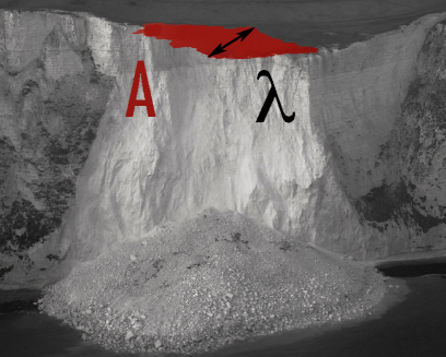
Figure 1: Idealization of an erosion event and definition of the measures of interest in this work: horizontal area at the cliff top, $A$, and maximum local retreat, $\lambda$.

In 2006, Teixeira reported [Teixeira, 2006] the analysis on a data-set of 140 failure events observed along the Algarve cliffed coast, between Porto de Mós beach and Olhos de Água beach, during nine years. Between July 1995 and June 2004, the average loss of horizontal area was 410 $m^{2}$/year, the mean annual volume was 9760 $m^{3}$, and the average recession rate was 0.9 cm/year. Besides average yearly measures, Teixeira analyzes the statistics of several linear quantities measured on each single erosion event: mean and maximal length (of coast interested by the failure), mean and maximal width (of the top cliff area interested by the failure, in the direction normal to the coastline), mean and maximal height (of the failure). The maximal width measured by Teixeira corresponds to what is noted here by $\lambda$ (see Fig. 1). From these quantities, Teixeira computes estimations for the horizontal area of loss (as the product between mean width and mean length). Interestingly, a strong correlation between the collected measures is observed, which seems compatible with a power law fit. For instance he reports a power law correlation between the horizontal area and the maximal width (maximum local retreat), with an exponent close to $1.75$: $A\propto\lambda^{1.75}$. Moreover, the cumulative frequency size statistics of the erosion events are performed, paying attention to the completeness of the inventory and comparing the results with an older inventory (from aerial photos) by Marques [Marques, 1997]. Despite the small number of events available (only the larger 69 single events), Teixeira manages to obtain an inverse power law fit with an exponent about $-1.37$ for the cumulative distribution of $\lambda$. We recall that the probability density $p(x)$ is equal to (minus) the derivative of cumulative distribution $P_{>}(x)$. Then, a power law decay of the cumulative with an exponent $\gamma$ corresponds to a power law decay of the probability density with an exponent $\gamma-1$. Here, the frequency decay for large failures should be: $f(\lambda)\propto\lambda^{-2.37}$.

Two years later, Marques [Marques, 2008] pushes the analysis further, considering twelve data-sets, including the one studied by Teixeira, but also the statistics of erosion events from other sections of the south-west coast of Portugal, as well as a small portion of Morocco coast (see [Marques, 2008] for the exact location of the cliffs). The inventories, containing from $10$ to $147$ data points each, for a total of of $650$ cliff failures, are relative to different coast sections, time period and collection methods (aerial photos, field photos and field survey).

The author analyzes the statistics of horizontal area ($A$), maximum local retreat ($\lambda$) and volume of the mass movements, by means of frequency-size distributions. The histograms of each data-set has been normalized to the respective total number of events, with the aim to proceed to a single fit over all the available data. The resulting distributions are studied in terms of log-binned histograms, which appear to spread over several decades. Again, both for the horizontal area and for the maximum local retreat, negative power laws are observed for large sizes: $f(A)\propto A^{-1.08}$ and $f(\lambda)\propto\lambda^{-2.30}$. Note that the exponent assessed by Marques for the maximum local retreat agrees with the findings by Teixeira.

Alternatively, Marques proceeds to a different fitting protocol: he just plots all the histograms together, without normalization, and then he looks for a single power law distribution describing all the available data (obtaining slightly different exponents, respectively $-1.05$ and $-1.94$).

Marques also investigates the correlation between $A$ and $\lambda$. Interestingly his analysis, which does not involve binning, nor normalization issues, considers the scatter plot of all the failures showing their area $A$ versus the corresponding maximum local retreat $\lambda$. The graph revealed a quite impressive correlation: all the points seem to align along a single power law curve: $A\propto\lambda^{1.79}$. The exponent found by Marques is in striking agreement with the previous result by Teixeira, on a more limited data-set.

In a recent paper by Young et al. [Young et al., 2011], an analysis of a small portion of unprotected and slowly retreating coastal cliffs near Point Loma in San Diego, California, US, is reported. The authors collected cliff failures observed over $5.5$ years (about $130$ events). They report several cumulative distributions of landslide failure parameters (area, mean retreat, maximum retreat, and length). Since the authors provide their data in a table, we could perform a direct analysis of them. In general the data does not span a large range of values and the log-binned histograms show a bending at low values, similar to the roll-over observed in landslide distributions [Malamud et al., 2004a] (especially for the maximum local retreat $\lambda$). Performing a fit on the whole interval gives exponents quite different from a fit on the largest values (respectively $\lambda>3m$ and $A>10m^{2}$), which in turn are consistent with the fits performed by Young et al. [Young et al., 2011] on cumulatives for the same ranges. Interestingly, when one considers the scatter plot $A$ vs. $\lambda$, the small values bending seems disappear: a fit on the whole range gives an exponent very close to what observed by Teixeira and Marques: $A\propto\lambda^{1.77}$.

A summary of all these results will be recalled in the Discussion section. In particular all the exponents mentioned in the paper will be given in Table 1.

2 Framework of the study

2.1 Modeling highly fluctuating phenomena

In the previous section, we cited different modeling approaches to coastal erosion. A classification of these models has been proposed in [Lakhan and Trenhaile, 1989]. Accordingly, the attempt to reproduce a physical, scaled, realization of a coastal system, corresponds to a physical model. On the other hand, mathematical models try to describe coastal systems in a more theoretical way. (This class is broad and it could be useful to refine it.)

For instance, the work by Dong and Guzzetti [Dong and Guzzetti, 2005], who proposed the inverse power law distributions in order to characterize the statistics of retreats, can be considered as a mathematical statistical modeling. At first sight this approach can be regarded as purely descriptive. Nevertheless, it turns to be a fundamental step, especially when one is faced with a broadly distributed phenomena, characterized by fat tailed distributions. As we’ll explain below, in such cases the statistical model warns us that average measures are less meaningful than expected, whereas fluctuations could be the relevant quantities to look at.

Before proceeding, we wish to stress some general features of fat tailed distributions, in particular power laws. The very first observation with broadly distributed random variables, is that their fluctuations are much larger than the standard (Gaussian or Poissonian) case. This doesn’t only mean that we need larger samples to get clean statistical results, but it can have more severe consequences. To clarify this point, the case of power law distributions is paradigmatic. Consider for instance a random variable $x$, whose density of probability distribution decays, for large $x$, as:

$$p(x)\propto x^{-\alpha}.$$

Obviously, moments of order larger than $\alpha-1$ diverge:

$$M_{n}=\int_{0}^{\infty}x^{n}p(x)dx=\infty\mbox{ for }n\geq\alpha-1.$$

This implies that for $\alpha<3$, the expected average ($M_{1}$) and variance ($\sqrt{M_{2}-M_{1}^{2}}$) are, in some sense, ill defined quantities. This observation has a direct consequence on the statistical analysis on finite samples. In the standard case (i.e. for distributions with rapidly, say exponentially, decaying tails) the empirical average over a sample rapidly converge to the expectation (i.e. the first moment) of the distribution (large numbers theorem). One can understand this behavior, since in this case when we add a number $N$ of random values, they equally contribute to the sum, giving a mean contribution which grows with $N$ and fluctuations around this mean of order $\sqrt{N}$. The empirical average, which is the sum divided by $N$, picks exactly the mean value of the sum, killing the contribution of the fluctuations.

For fat tailed distributions the scenario can be completely different. For instance, for a power law distribution with exponent smaller than $3$, the sum of $N$ random values is typically dominated by the few largest values, which overwhelm the rest of the terms. This is a consequence of slow decaying tails, giving a relatively large probability to large values. In this case, the empirical average can be highly fluctuating and depends dramatically on the sample size. More precisely it can be shown [Gumbel, 1958] that the largest on a sequence $x_{1}$, $x_{2}$, …, $x_{N}$ of $N$ values typically grows as $N^{1/(\alpha-1)}$, and consequently the empirical average $\langle x\rangle_{N}$ grows as $N^{(2-\alpha)/(\alpha-1)}$, which diverges for $1<\alpha<2$. Similar arguments show that when $2<\alpha<3$, it is the variance that does not exist (the standard deviation diverges for increasing sample size).

The reason why power laws govern many physical phenomena, is a very general issue. To frame the problem, it is worth recalling that probability distributions can be separated into two distinct categories: stable and non stable distributions. A probability distribution is stable if the sum of two (or more) independent variables thrown from it follows the same probability distribution. Roughly speaking, there exists only two types of stable laws: the Gaussian law and power laws (Levy distributions). For instance, the sum of independent, Gaussian random variables follows again a Gaussian distribution. The case of power laws has a more specific interest here, for if the distribution of masses of elementary rock falls obeys a distribution whose tail decays as a power law (with an exponent between $1$ and $3$), the distribution of the sum of $N$ falls should obeys a power law with the same exponent.

2.2 Consequences on the average erosion rate

A power law in the distribution of retreats can have serious consequence on the long term erosion rate. Let’s reason in terms of the stochastic model presented by Hall et al. in [Hall et al., 2002]. The average retreat rate measured on a time $t$ is defined as

$$R(t)=\frac{\sum_{i=1}^{N}C_{i}}{t}$$

where $N$ is the number of events observed in the time window $t$. Now, if there is a finite mean time $\tau$ between erosion events, as suggested by Hall in [Hall et al., 2002] (where $\tau=k\lambda$), then

$$R(t)=\frac{\sum_{i=1}^{N}C_{i}}{N}\frac{N}{t}\approx\left(\frac{1}{\tau}\right)\langle C\rangle_{N}.$$

with $N\approx t/\tau$. In this case, the average erosion rate, would scale as the average of a sequence of $N=t/\tau$ erosion events. If the distribution of retreat events $p(C)$ is a power law (as suggested by Dong and Guzzetti [Dong and Guzzetti, 2005]), the measured value of this quantity, as well as their statistical fluctuations, critically depends on the power law exponent. For small values of the exponent, the average erosion rate depends on the time window where it is computed, and the very concept of a long term average erosion rate no longer makes mathematical sense (see Fig. 2).

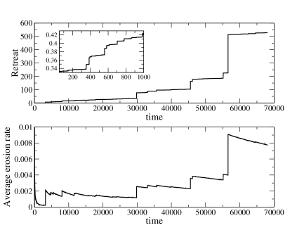
Figure 2: ST-model, similar to the model presented by Hall et al. [Hall et al., 2002], but with power law distributed retreat lengths (decay exponent equal to $1.5$). Upper panel: the retreat (arbitrary units) as a function of time (arbitrary units). Note the highly episodic dynamics, which reproduces similar jumps at every scale (in the inset, a zoom of the first 1000 time steps). Lower panel: average erosion rate as a function of elapsed time. Note that the average is ill defined, since it depends of the time windows and does not converge to a constant at large time.

This discussion suggests that the model for $p(C)$ is crucial for the interpretation of the phenomenon. In particular, for very fluctuating phenomena, average quantities could be ill defined. On the other hand, the study of fluctuations may turn to be quite interesting and models as the one proposed by Hall [Hall et al., 2002] (see also [Crowell et al., 1997, Amin and Davidson-Arnott, 1997]) could be very useful tools. We adopt the name of stochastic models for similar studies, since these models are standard in stochastic processes theory (for instance the model by Hall is a renewal process [Feller, 1978]). Stochastic models make use of statistical models in order to define a stochastic process describing the fluctuating nature of the observation. These models, below referred as ST-models, allow to produce a synthetic succession of erosion events through numerical simulation of a stochastic process. The analysis of such numerical data can be compared with field observations, or adapted to them via Bayesian parameter estimation, and hopefully used for expert assessment of local analysis.

However, both statistical and stochastic models still lack of a more grounded, physical justification. Some authors [Teixeira, 2006] noted that “the physical reason as to why the width frequency of slope mass movements satisfy the power-law is uncertain, since it depends on the complex relation between the internal characteristics of the rock masses and the slope mass movements triggers. The best single explanation takes into account the relationship stated by Malamud et al. (2004) [Malamud et al., 2004a] between landslide event magnitude and trigger magnitude. Retreat of cliffs or coastal bluffs is greatly dependent on the frequency of wave attack on cliff toe and on the rain intensity, which are triggering factors that obey themselves power laws.” [Teixeira, 2006]. In the following we provide arguments for a different origin of the observed power laws, related to the “critical” nature of the erosion process.

2.3 Scale invariance

Another mathematical property of power laws, is that they are homogeneous function, i.e. that they satisfy a multiplicative scaling, i.e.

$$f(lx)=l^{k}f(x).$$ (4)

This means that a change of scale of the quantity $x$ results in a change of scale in the value of $f$, with an appropriate exponent. Vice versa, it’s easy to show, choosing $l=1/x$, that Eq. 4 implies that $f(x)$ is a power law: $f(x)=f(1)x^{k}$.

Knowing the scaling behavior of a function is very useful in order to get its expression. In ordinary geometry, we know that if we double the radius of circle, its area will be four times larger, i.e. it will scale by $2^{2}$ (the surface is an homogeneous function of the radius, with $k=2$). This implies that the area is proportional to the square of the radius.

Nature produces more complex geometrical objects. River network basins, for instance, are known to satisfy Hack’s law [Hack, 1957]: if one consider the length $l$ of the main stream of a river basin as a function of the basin area $a$, it turns that in average:

$$l\propto a^{h},$$ (5)

where $h$ is about $0.6$.

An other geomorphological example is provided by rocky coasts. In several cases it has been observed [Mandelbrot, 1967] that coastlines are fractal, a property which can be expressed as a scaling of the length $L$ of the coast between two points as a function of the distance between the points $d$

$$L(d)\propto d^{D_{f}}.$$

The exponent $D_{f}$, the coastal fractal dimension, is often around $1.3$, but it may attain higher values for fjorded coasts [Baldassarri et al., 2008].

For both cases, river networks and rocky coasts, the appearance of power laws in their geometrical characterizations has a striking visual counterpart. If we look at the map of a fractal coast, as well as at a picture of a river network, is very difficult to guess its scale, if it is not explicitly mentioned in the map, or if there are no known objects (houses, trees) to compare. This property is generally known as “scale invariance”, and indicates the absence of a characteristic length in the system.

Even the geometry of coastal erosion events seem to display non trivial scaling properties. As reviewed in the introductory section of this paper, the available studies [Teixeira, 2006, Marques, 2008, Young et al., 2011] suggest that the horizontal area of the eroded cliff top area $A$ scales in average as a power of the maximum local retreat $\lambda$, i.e.

$$\bar{A}\propto\lambda^{\nu},$$ (6)

where the exponent $\nu$ is around to $1.8$, and $\bar{A}$ is the average, or typical area $A$, of an erosion of retreat $\lambda$. The need for using the average $\bar{A}$ is due to the fact that the horizontal area $A$ is not a deterministic function of the retreat $\lambda$, and the relation (6) holds “on average”. To be more precise, one should consider that $A$ and $\lambda$ are random variables defined by their joint probability distribution $P(A,\lambda)$, which is unknown, and the average $\bar{A}$ is computed using the conditional probability $P(A|\lambda)$ (i.e $\bar{A}$ is the conditional average $E\left[A|\lambda\right]$).

Nevertheless, we may have access to the (marginalized) distribution $P(A)$ and $P(\lambda)$. Observations from catalogs indicate that, in a measurable range of values, both quantities seem to present a power law distribution, which defines two other exponents:

$$P(\lambda) \propto \lambda^{-\eta}$$ (7)

$$P(A) \propto A^{-\alpha}.$$ (8)

As we’ll show in the following, if the scenario depicted by Eqs. (6), (7), (8) is confirmed, then it is possible to propose a simple scaling hypothesis on the conditional probability distribution that gives a relation between the three exponents. In other words, the three values $\nu$, $\alpha$, $\eta$ are not independent, and their relation can be useful to check the consistency of the measured exponents.

Scaling relations for power law exponents, obtained via scaling hypothesis similar to what will be proposed here, has been the starting point for very fruitful investigations in the statistical physics of critical phase transitions [Fisher, 1967, Kadanoff et al., 1967]. The deep reason for this is that near critical points (Curie temperature for magnetic materials, critical point for vapor-liquid transition, superconductive transition, super-fluid transition, etc) physical systems display a form of “scale invariance”.

In this context it has been possible to understand the occurrence of power laws, to compute analytically their exponents and to identify class of phenomena which should obey the same laws (universality classes). In order to achieve this result, models have been proposed, which consider only some very basic, minimalist ingredients of the real, complex, physical system. Nevertheless, such models correctly and quantitatively describe specific critical behaviors (for instance power law exponents) of a large and diverse class of natural systems.

In this spirit, a statistical physical model (SP-model) for the erosion of rocky coasts has been proposed [Sapoval et al., 2004], aimed to describe the observed large scale geometry of rocky coasts, including, but not limited, to fractal coasts [Baldassarri et al., 2014]. Here we show that the same model can give insights on the statistics of erosion events. The relevance of such approach is to give a rationale for the observation of power laws. Moreover, the model allows to relate the coastal erosion process to the universality class of percolation phenomena, and it opens the possibility of a direct computation of some exponents characterizing the erosion statistics.

In the following, we propose a scaling hypothesis which reproduce the general statistical features of present catalogs. Finally, we present extensive numerical simulations of the SP-model [Sapoval et al., 2004] for rocky coast erosion, which produce, without adjustable parameters, power laws directly comparable with the observed ones.

3 Results

3.1 Scaling relation between exponents

The correlation observed between $A$ and $\lambda$, should reflect a dependence on the probability distributions of $A$ and $\lambda$. As a first crude approximation, one can consider $A$ as a deterministic function of the random variable $\lambda$, where

$$A(\lambda)\propto\lambda^{\nu}.$$ (9)

In this case, it is straightforward to obtain the distribution $P(A)$ from the distribution $P(\lambda)$, since:

$$P(A)=P(\lambda)\left|\frac{d\lambda}{dA}\right|.$$

This implies that if $P(\lambda)$ decreases as a power law for large $\lambda$, the same would happens for $P(A)$ and corresponding decay exponents would be related by the equation:

$$\eta-1=(\alpha-1)\nu.$$ (10)

Eq. (9) is a very strong assumption and, as explained above, it should rather be recast in terms of the (conditional) average of $A$, which is a random variable fluctuating around this mean. Nevertheless, it’s quite simple to generalize the computation, making use of a simple scaling hypothesis on the conditional probability $P(A|\lambda)$, which is nothing but $P(A,\lambda)/P(\lambda)$:

$$P(A|\lambda)=\lambda^{\nu}F\left(\frac{A}{\lambda^{\nu}}\right),$$ (11)

where $F$ is an arbitrary probability distribution. As detailed in the Appendix A, the computation leads exactly to the same Eq.(10).

3.2 Statistical physical model for rocky coast erosion

Here we present the statistics of erosion events generated by numerical simulations of a particular SP-model, whose detailed definition appeared elsewhere [Sapoval et al., 2004]. The basic idea of the model is to consider the coast (and the inland) as a random medium, i.e. characterized by local random numbers $r_{i}$ (where $i$ are the geographical coordinates of the site) which measure the resistance to sea erosion. When a site is exposed to the action of the sea, its resistance $r_{i}$ is compared with an average sea erosion force $f$ and eroded if $f>r_{i}$. This extreme simplification of the coastal system is slightly articulated: by one side considering that the resistance $r_{i}$ takes into account a principle of local mechanical stability (resistance is smaller if the site is not protected or sustained by neighbors, i.e. it decreases together with the number of neighboring rocky sites). On the other hand the sea force is not constant in time, but responds to the damping effect of the coastal geometry: $f$ is smaller for irregular coastlines, i.e. with bays and headlands, than in the case of a straight shoreline.

The numerical implementation of the model [Sapoval et al., 2004] (see appendix B for details) shows that such simple ingredients put in place a feedback mechanism: eroding the weaker parts of the coasts, the sea may increase the irregularity of the coastline. A larger irregularity, in turn, increases the damping of the sea force and, hence, slows down sea erosion. The result of this dynamics (called “fast erosion” in [Sapoval et al., 2004]) is the emergence of a stable coastline, whose local resistances are everywhere stronger than the current sea erosion force.

The geometry of this stable coastline has been extensively studied: it depends on the importance of the damping (determined by the only parameter of the model, called “gradient”) and can be directly related to the geometry of a well known fractal mathematical object, the accessible external perimeter of the critical percolation cluster [Grossman et al., 1987, Stauffer and Aharony, 1991], whose dimension has been demonstrated equal to $4/3$ [Duplantier, 2000, Lawler et al., 2004, Schramm, 2006]. Nevertheless, the model is not restricted to fractal coasts, since full fractality develops only in the case of very small gradient.

In the current study, we consider a stable coast as the starting point for the collection of erosion events. The coast is supposed to come from previous erosion which means that the coast is constituted by a collection of ”strong” rocks that all present a resistance to erosion $r_{i}$ that are, by definition, larger than the sea erosion force $f$.

Then we proceed to simulate a “slow weathering” process: i.e. we progressively weaken the exposed rocks until a single site becomes fragile (i.e. its resistance $r$ is smaller than $f$). This triggers a new fast erosion dynamics that keeps going until a new stable coast is found. When the coast is again stable against erosion, we identify the connected sets of sites [Hoshen and Kopelman, 1976] just eroded and we compute for each their surfaces $A$ and their maximum local depth $\lambda$.

We perform extensive numerical simulations, for large systems ($L_{0}$ larger than $10^{4}$) collecting a large number of erosion events (larger than $10^{6}$), for several values of the gradient parameter $g$ (see Appendix B for details).

In Fig. 3, we show some statistics obtained for the area $A$. We observe that the power law decay is mostly independent from the value of the gradient, which rather controls the range where the power law decay applies. As expected from previous studies [Sapoval et al., 2004], the smallest the gradient, the larger the range where scale invariance (hence power law decay) applies. The gradient parameter $g$ controls the largest characteristic scale in the system, i.e. the geometrical correlation length of the coastline. This length, in turns, corresponds to the largest erosion size typically observed. In other words, $g$ controls the cut-off at large size of the power law decay of both $A$ and $\lambda$: the smallest $g$, the broader the power law range in the distributions.

In particular, simulation of the smallest $g$ value, produced more than $10^{6}$ erosion events and a very clear power law decay, without any observable cut-off at large sizes. Thanks to the extensive statistics, we obtained a good estimation of the decay exponents, quite insensible to binning or to the range of fitting (even if for small sizes, some spurious effects due to the lattice geometry are observed). The results are: for the frequency of horizontal area (see Fig. 4, left)

$$f(A)\propto A^{-1.71};$$

for the maximum retreat length (Fig. 4, right)

$$f(\lambda)\propto A^{-2.32};$$

for the correlation between the two, i.e. the conditional average $\bar{A}=E[A|\lambda]$ as a function of $\lambda$ (Fig. 5):

$$\bar{A}\propto\lambda^{1.82}.$$

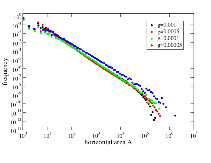
Figure 3: Horizontal area distribution of erosion events produced by extensive numerical simulation of the SP-model. Simulation parameters are $L_{0}=20000$ for different values of $g$ (as noted in the figure legend). All simulations started from a flat coastline with an initial sea force strength of $0.6$ and proceeded for millions of successive weakening triggerings of erosion events, for each value of $g$. For each curve, the frequency is scaled by an arbitrary factor in order to keep the different curves closer, for slope comparison.

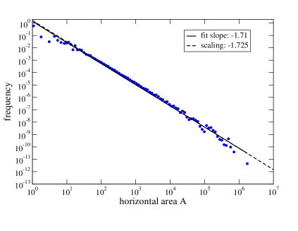
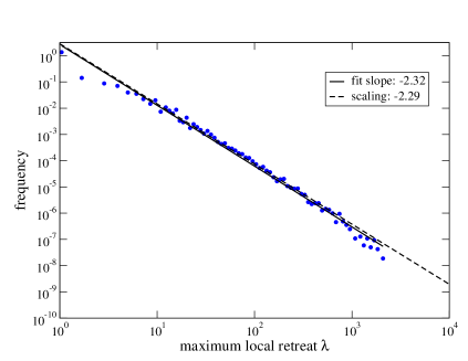
Figure 4: Distribution for horizontal area $A$ (left) and maximum local retreat $\lambda$ (right) for the SP-model, with $g=5\cdot 10^{-5}$, from more than $10^{6}$ erosion events. Simulation for a system with lateral dimension $L_{0}=20000$ and an initial sea force strength of $0.6$. The black solid line is a numerical fit, while the dashed line is the scaling prediction given by Eq. (10).

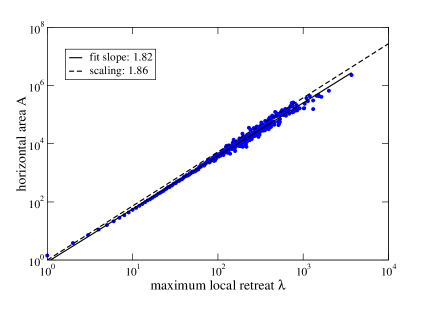
Figure 5: Conditional average $\bar{A}=E[A|\lambda]$ for the SP-model, with $g=5\cdot 10^{-5}$, from more than $10^{6}$ erosion events. Simulation for a system with lateral dimension $L_{0}=20000$ and an initial sea force strength of $0.6$. The black solid line is a numerical fit, while the dashed line is the scaling prediction given by Eq. (10).

4 Discussion

4.1 Fit comparison

As for landslides [Hovius et al., 1997, Hartshorn et al., 2002, Malamud et al., 2004b, Brunetti et al., 2009], cliff erosion statistics display broad distributions, when one considers the decay of the frequency as a function of magnitude of erosion events. Despite the limited statistics available, this statement is no more just a claim. We think that the work by Marques [Marques, 2008] leaves no much doubts about it. In Fig. 6 we reproduce his best results, i.e. the normalized histograms for the distribution of $A$ (left) and $\lambda$ (right). Despite the obviously noisy aspect, the distributions span several decades of sizes. The straight black lines reproduce the fits by Marques on large events.

Let look at the distribution for $\lambda$, i.e. the plot at the right in Fig. 6. Marques performed the fit for the $\lambda$ distribution “for movements with maximum local retreat higher then 2 m” [Marques, 2008]. The corresponding exponent is in remarkable agreement with the fit obtained on the statistical analysis of our model (as well as with the exponent previously measured by Teixeira on his catalog [Teixeira, 2006]). In fact the two fitting curves (straight black and staggered red line) are indistinguishable in the plot.

Now consider the distribution for $A$, shown in the left plot in Fig.. 6. In this case, the fit by Marques (black straight line) and the fit from our model (red staggered line) differ. However, Marques apparently performed his fit on the whole data range available. This procedure is not coherent with the previous fit, though. One should rather consider only events of area, say, larger than $3-4$ m²: smaller sizes should correspond to the movements dropped in the previous fit. Apparently, the exponent obtained with our SP-model is much closer to the decay of $A$ in such a range, even if a direct comparison is not easy. In the following we’ll propose another argument in favor of such interpretation (see below).

Finally, Fig. 7 representing the correlation between $A$ and $\lambda$ doesn’t seem to suffer for such limitations, and the fit on the whole range performed by Marques seems quite reasonable. Again the resulting exponent impressively coincides with the one obtained from our SP-model.

A similar discussion applies for the Californian catalog distributions by Young et al., see Fig. 8. The poorer statistics makes the histograms noisier and an evident roll-over appears for small sized events. Again the exponents obtained with our SP-model seem to be compatible with the large size decay of both distributions, but fail at smaller range (say $\lambda<3$m and $A<9$m²). Nevertheless, if one consider the correlation between $A$ and $\lambda$, in Fig. 9, roll-over effects disappear and a power law seems quite reasonable. Again the corresponding fit on the Californian catalog data agrees fairly well with the exponent obtained by our SP-model.

Here we stress that in our SP-model the observation of power laws is directly related to the (self) critical nature of its dynamics. Only the range of the power law decay could eventually be reduced by the size of the lattice width $L_{0}$ or by a large value of the gradient parameter $g$. For small values of $g$, where power laws are evident, the fitted exponents are uniquely determined and independent from $g$, as well as other model parameters. Moreover, as it has been noted elsewhere [Desolneux et al., 2004], (gradient) percolation models, as the SP-model used here, performs very well in exposing their critical properties even for large gradients. This seems the case for the correlation between $A$ and $\lambda$, both for the model and for the geometry of real cliff collapses.

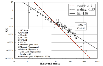
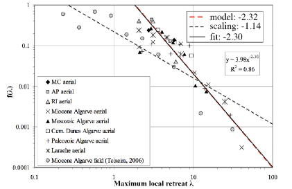
Figure 6: Horizontal area (left) and maximum retreat length (right): magnitude-frequency analysis, from [Marques, 2008] (normalized histograms). The lines represent the fit performed by Marques (black solid line), and the slopes obtained using Eq. (10) (dashed black line) and a the SP-model (dashed red line).

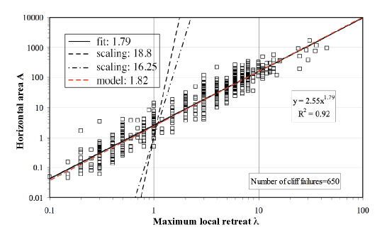
Figure 7: Horizontal area vs. maximum local retreat, from [Marques, 2008]. The lines represent the fit performed by Marques (black solid line), and the slopes obtained from Eq. (10), using the values of $\alpha$ and $\eta$ obtained by Marques fitting normalized and non normalized histograms (respectively, dot-dashed and dashed black line). The dashed red line show the slope from the SP-model.

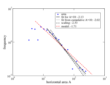
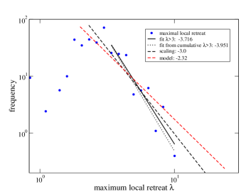
Figure 8: Horizontal area (left) and maximum local retreat (right) distributions for Californian erosion events [Young et al., 2011]. The black straight and dotted lines represent respectively slopes from fit on histogram and on cumulative distribution, for large events only ($A>10$m²). The black dashed line is the slope computed via Eq. (10), while the red dashed line is the slope from our SP-model.

Figure 9: Horizontal area versus maximum local retreat for Californian erosion events [Young et al., 2011]. The black straight line represent the fit on the whole range of data. The black dashed line is the slope computed via Eq. (10), while the red dashed line is the slope from our SP-model.

4.2 Scaling laws

Here we discuss how to use Eq. (10), relating the values of the exponents $\alpha$, $\eta$, and $\nu$, as a check for the fit from catalog data. Using Eq. (10), given two of the three exponents, the third can be predicted, as shown in Table 1 for all the exponents mentioned here.

A quick way to judge the consistency of the fits could be to consider the relative deviation of the measured fit from the scaling prediction. If the deviation is large, one should suspect that at least one of the two exponents used for the prediction has a problem.

For instance, considering the results by Marques [Marques, 2008], summarized in Table 1, the exponent which has the smallest deviation from the scaling prediction is the value of $\alpha$. On the contrary, the prediction for the value of $\lambda$ differ by almost the $50\%$ from the measured exponent, while the prediction of $\nu$ is astronomical! This strongly suggests that the value of $\alpha$ coming from the fit by Marques, whose value is close to $1$, undervalues the real exponent, which should be closer to the scaling predictions $1.7$ (close to the SP-model value).

Another use of the scaling hypothesis, which results in relation Eq.(10), is to improve the stochastic model approach proposed by Hall et al. [Hall et al., 2002]. In fact, it could be useful to have a stochastic model describing the variety of measures characterizing cliff collapses, rather than just a generic retreat length. For instance it could be useful to generate synthetic statistics of erosion events, in terms of their horizontal area and the maximum local retreat. Obviously these two quantities are statistically dependent and one should not simply use the observed single variable distributions $P(A)$ and $P(\lambda)$, but take in consideration the full joint probability distribution $P(A,\lambda)\neq P(A)P(\lambda)$. This can be done, through the conditional probability, since

$$P(A,\lambda)=P(\lambda)P(A|\lambda),$$ (12)

making the scaling assumption on the $P(A|\lambda)$ in Eq. (11). For instance, choosing for the scaling function $F(x)$ a simple exponential, it is possible to generate the area $A$ and maximum local retreat $\lambda$ of a random event using the following numerical recipe: 1) throw a random number $r_{1}$ uniformly distributed between zero and one; 2) put $\lambda=\lambda_{0}x^{1/(1-\eta)}$, in order to get $\lambda$ distributed as (7), where $\lambda_{0}$ is the minimal value for the random variable $\lambda$; 3) throw a second random number $r_{2}$ uniformly distributed; 4) put $A=A_{0}-\lambda^{\nu}\log r_{2}$ in order to get $A$ distributed as (8) and correlated with $\lambda$ as to give (6). ($A_{0}$ fixes the minimal value for the random variable $A$).

It is simple to refine this procedure in order to introduce roll-over effects on the distributions $P(A)$ and $P(\lambda)$, or to generalize it to a larger number of random variables, as for instance the volume displaced $V$, which also presents power law correlations with both $A$ and $\lambda$ [Teixeira, 2006, Marques, 2008] .

5 Conclusions

In this work we have discussed various aspects of the statistics of rocky coast erosion. As many geological processes, coast erosion acts on many time scales and on broad length scales. Several works have convincingly raised the hypothesis of power laws in the distribution of cliff failure sizes. We tried to put together different observations in a tentative coherent framework. In particular, we note an interesting convergence by different researchers on a geometrical characterization of erosion events, which relates the horizontal area lost at the cliff top with the maximum local retreat. Such a relation defines a “geometrical exponent” $\nu$, whose value turns to be around $1.8$. More difficult is the measure of the decay exponents $\alpha$ and $\eta$ of distributions, respectively, for the area and for the maximum retreat.

However, it is quite easy to obtain a relation between the three exponents, based on simple scale invariance hypothesis. In other words, the three exponents are not independent, and we discussed in details how this result could be used to improve both the analysis and modeling of cliff failure statistics. In Fig. 10, we show to what extent the actual measures of the decay exponents $\alpha$ and $\eta$ agree with the scaling law in Eq. (10), given the corresponding measure of $\nu$. We judge the result quite fair, considering the scarce statistics from which the exponents are measured (see the last row of Table 1).

In a totally different step, we develop what could be called a toy model of sea erosion, in which the resistance to erosion of the rocks are distributed randomly but the rocks are submitted to a sea erosive power that decreases due to energy damping along a more irregular coast. The spontaneous evolution of such a system leads to an irregular and stable coastline, which, under the action of slow weathering or storms, undergoes to an episodic sequence of erosion events. The important point here is that, taking an earth constituted by random rocks, the sea erodes the weaker rocks, up to reaching a set of strong rocks. Nevertheless, behind this resistant shield of strong rocks, it lies a disperse, random lithology which has not yet experienced the action of the sea. In other words, our model recognize in the coastline a strong, but fragile barrier to sea erosion. A slight, local increase of the erosion force, as well as the weakening of the resistance of a single coast site, is able to trigger an erosion event of possibly large size, which locally redesigns the coast, in order to identify a new resistant coastline.

Using this toy model we collect large sequences of erosion events. We study their geometry and compute their statistics, to be compared with real data from existing catalogs. We find power laws with exponents that resemble those observed on the field. For instance, the geometrical exponent obtained with our model ($\nu=1.8$) is very close to the value at which several independent observations converge. Moreover, thanks to the large statistics attainable with our numerical simulations, we show that the scaling relation Eq. (10) between the three exponent is satisfied by this toy model (see Fig. 10). Such a result, however, was highly expected, since our model possesses some scale invariant features, typical of critical phenomena, which justify the scaling hypothesis on its probability distributions. More specifically, our toy model pertains to the large class of percolation critical phenomena.

Percolation theory, a breakthrough in the physics of critical systems, deals with the geometry of random connected sets of sites stronger than a burning agent or an infiltrating substance. Quite interestingly, our model seems to relate percolation to the large scale erosive action of the oceans on continents.

Note two important aspects of our results. Firstly, many details of the numerical implementation of the model are known to be irrelevant, with respect to the measured exponents (geometry of the lattice, distribution of lithology, several dynamical rules etc.). This property descends from the fact that our model of rocky coast erosion belongs to the percolation universality class, identified exactly by the value of the exponents of power law distributed quantities (critical exponents).

Secondly, our model does not need a fine tuning of external parameters: the only parameter of the model (the gradient) determines the maximum size of observed failures, but does not change the exponents of the produced power law statistics. This makes our model an example of what is called ”self-organized criticality”.

We recall that the connection between percolation and coast geometries has been recently invoked by independent studies [Boffetta et al., 2008, Saberi, 2013]. Here, we show how the coastal erosive dynamics could represent an other, important hook to corroborate such a link.

Beyond its conceptual and theoretical value, these results open interesting perspectives for future studies. For example, the scaling relations between several measured exponents, similar to the one proposed here, could be used as a benchmark for the coherence of the statistical description of catalogs, as well as a possible source of prediction for missing or scarce statistics. This also suggest that further investigations on the geometrical characterization of erosion events, could be useful to relate different quantities and their probability distributions. This is not strictly related to rocky coast erosion, but could also be useful in other highly fluctuating processes, as, for instance, in landslide statistics.

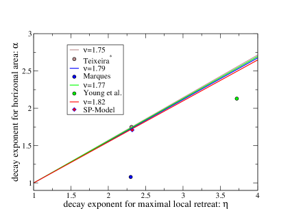
Figure 10: Values of decay exponents $\alpha$ and $\eta$ for the main measures described in the paper. Each point should be compared with the line of the same color, representing the scaling prediction from Eq. (10) with the corresponding measured value of $\nu$. Note that: the value of $\alpha$ for Marques [Marques, 2008] may be an underestimation (see discussion), the value by Teixeira [Teixeira, 2006] is computed by Eq. (10) and the exponents for Young et al. [Young et al., 2011] may suffer for large roll-over effects.

Summary of results for the decay exponents of density probability distributions
Measure [exponent]	Algarve I	Algarve II	San Diego	SP-model
Area $A$ [$\alpha$]	- (1.75∗, 2.21+, 2.19o)	1.05a (1.52) - 1.08b (1.73)	2.13 (2.53)	1.71 (1.72)
Max. loc. retreat $\lambda$ [$\eta$]	2.31∗, 3.13+, 3.09o (-)	1.94a (1.09) - 2.30b (1.14)	3.72 (3.00)	2.32 (2.29)
$A$ vs $\lambda$ [$\nu$]	1.75 (-)	1.79 (18.80a - 16.25b)	1.77 (2.40)	1.82 (1.86)
Sample size	140	650	130	$>10^{6}$

Table 1: Table of exponents collected in this work. Each exponent has predicted values (in brackets), obtained with scaling relations Eqs. (8), (7) and (6), using the fitted values for the other two exponents. Second column (Algarve I) from [Teixeira, 2006]: The exponent $\eta$ is recovered from the fit on the cumulative frequency distribution(frequency density exponent = cumulative frequency exponent - 1). The values reported are for a recent field inventory ^∗, an historical photographic inventory ⁺ and for the assembled inventories normalized for an annual frequency ^o. No fit for the exponent $\alpha$ are reported in [Teixeira, 2006], but we could provide the prediction via scaling equation Eq. (10). No predictions are possible for exponents $\eta$ and $\nu$. Third column (Algarve II) from [Marques, 2008]: exponents marked with ^a are from unnormalized histograms, while those with ^b are form normalized histograms. Fourth column (San Diego) are the exponents computed from the data in [Young et al., 2011], on the whole range available. This procedure give poor results for $\alpha$ and $\eta$ (due to evident roll-over effects), while seems reasonable for $\nu$. Fifth column (SP-model) are from the numerical simulation presented in this paper (see figures from Fig. 4 to Fig. 5).

Appendix A Scaling hypothesis and scaling relation

We start from the conditional average of $A$ with respect to $\lambda$, defined as

$$E\left[A|\lambda\right]=\int_{0}^{\infty}AP(A|\lambda)dA,$$

where $P(A|\lambda)$ is the conditional probability (Eq. (12)). We assume that this quantity shows a power law behavior $E\left[A|\lambda\right]=C_{1}\lambda^{\nu}$. This feature is reproduced if $P(A|\lambda)$ has the simple scaling form given in Eq. (11), where $F$ is an arbitrary probability distribution function ($C_{1}$ turns to be its first moment).

The second assumption is that $\lambda$ has a power law distribution, at least in a range $\lambda_{0}<\lambda<\lambda_{*}$. This can be expressed as

$$P(\lambda)=\lambda^{-\eta}G\left(\frac{\lambda}{\lambda_{*}}\right),$$ (13)

where the scaling function $G(x)$ is almost constant in the range $x_{0}=\lambda_{0}/\lambda_{*}<x<1$. $\lambda_{*}$ represents the typical largest a value of $\lambda$ observed and, hence, $G(x)$ decreases rapidly (exponentially) to zero for $x>1$. The value $\lambda_{0}$, instead, is a lower limit for the power law range and the function $G(x)$ at small $x<x_{0}$ controls the behavior of $P(\lambda)$ for small $\lambda$, being possibly responsible for roll-over effects. Obviously, the measure of the exponent $\eta$ will be the better the larger $\lambda_{*}$ with respect to $\lambda_{0}$, that is the broader the power law range. The hypothesis expressed in Eq. (11), together with the observation in Eq. (13), gives a prediction for the joint distribution

$$P(A,\lambda)=\lambda^{-(\nu+\eta)}F\left(\frac{A}{\lambda^{\nu}}\right)G\left(\frac{\lambda}{\lambda_{*}}\right),$$

from which we can compute $P(A)$, which, making use on the hypothesis on $G(x)$, can be written in the form

$$P(A)=A^{-\frac{\nu+\eta-1}{\nu}}H\left(\frac{A}{A_{*}}\right),$$

where $A_{*}={\lambda_{*}}^{\nu}$. It’s not hard to see that the scaling function $H(x)$ is almost constant for $x\ll 1$. This means that $P(A)$ manifests, in this range, a power law with an exponent $\alpha$ related to $\eta$ and $\nu$ through the scaling relation Eq. (10).

Appendix B Model implementation

There can be several different numerical implementation of the ideas inspiring our model. Here the land is described by a square lattice of random units of global width $L_{0}$. Each site represents a small portion of the earth, named a rock in the following. The sea acts on a shoreline constituted of these rocks, each one characterized by a random number $l_{i}$, uniformly and independently distributed between $0$ and $1$, representing its lithology. The erosion model should also take into account that a site surrounded by the sea is weaker than a site surrounded by earth sites. Hence, the resistance to erosion $r_{i}$ of a site depends on both its lithology and the number of sides exposed to the action of the sea. This is implemented here through the following rule: sites surrounded by three earth sites have a resistance $r_{i}=l_{i}$. If in contact with $2$ sea sites the resistance is assumed to be equal to $r_{i}=l_{i}^{2}$. If site $i$ is attacked by $3$ or $4$ sides, it has zero resistance. This last prescription can be also seen as a minimal implementation of a principle of mechanical stability for the lithological units.

The sea erosion force $f$ is assumed to be the same along all the coast sites, and the damping due to the coast morphology is implemented taking into account the total length of the coast (this is inspired by studies of fractal acoustic resonator [Felix et al., 2007]). This results in a simple formula:

$$f=\frac{f_{0}}{1+gL/L_{0}},$$ (14)

where the crucial parameter is $g$ (the “gradient”), which measure the strength of the geometric damping effects. The constant value $f_{0}$ determines the force acting on a smooth, straight coast, whose length is $L_{0}$. (The value of $f_{0}$ is quite irrelevant for the following discussion, as far it is not smaller than the site percolation threshold of the lattice considered [Stauffer and Aharony, 1991]).

During the erosion dynamics, the value of the sea force $f$ is compared with the resistances $r_{i}$ of the exposed sites. When a site has resistance $r_{i}<f$, it is eroded, i.e. the rock is destroyed and the site invade by the sea. The erosion of a rock has several consequences. It expose new sites, previously in the inland, to the sea. It may change the resistances of the nearby rock sites (since they increase the sides attacked by the sea). Modifying the local morphology of the coast, it may change its total length, determining a change of the sea force $f$, which is updated according to Eq. 14.

Numerical simulations of the algorithm just exposed show that, after an irregular and a fluctuating dynamics of the coast geometry and the erosive force $f$, the process spontaneously stops identifying an irregular (fractal for small values of $g$), but strong coastline, resistant to further erosion.

The resistant interface so generated, can be weakened in several ways, in order to restart the dynamics and to produce erosion events. The choice here has been to uniformly decrease the resistance of every coast sites, until one of the site become weaker than the sea force $f$. Other triggering procedures can be put in place, but we predict that this would not change the main results presented here. Our choice for the triggering mechanism makes our dynamics similar in some sense to the so called invasion percolation model [Wilkinson and Willemsen, 1983].

The triggering let the erosion process start again. The erosion can remain local or (rarely) involve different spots along the coastline. Anyway, after a while, the sea erosion stops again. It is then possible to identify the set of connected eroded sites [Hoshen and Kopelman, 1976], called hereafter erosion event. We measure its surface (number of sites) and the largest size in the direction orthogonal to the average direction of the coastline: these are the equivalent of the horizontal area $A$ and the maximum local retreat $\lambda$ of the observed erosion. (Several definitions of maximum local retreat are possible, and this one does not strictly coincides with the one by Marques, who considers the depth orthogonal to the average direction of the cliff before erosion. However, in our model local erosion are mainly isotropic.)

References

- [Amin and Davidson-Arnott, 1997] Amin, S. M. N. and Davidson-Arnott, R. G. D. (1997). A statistical analy- sis of controls on shoreline erosion rates, Lake Ontario. Journal of Coastal Research, 13(4):1093––1101.
- [Baldassarri et al., 2008] Baldassarri, A., Montuori, M., Prieto-Ballesteros, O., and Manrubia, S. C. (2008). Fractal properties of isolines at varying altitude revealing different dominant geological processes on Earth. Journal of Geophysical Research, 113:E09002.
- [Baldassarri et al., 2014] Baldassarri, A., Sapoval, B., and Felix, S. (2014). A numerical retro-action model relates rocky coast erosion to percolation theory. Submitted to Geomorphology, arXiv:1202.4286.
- [Boffetta et al., 2008] Boffetta, G., Celani, A., Dezzani, D., and Seminara, A. (2008). How winding is the coast of Britain? Conformal invariance of rocky shorelines. Geophysical research letters, 35:1–5.
- [Brunetti et al., 2009] Brunetti, M., Guzzetti, F., and Rossi, M. (2009). Probability distributions of landslide volumes. Nonlinear Processes in Geophysics, 16(1):179–188.
- [Crowell et al., 1997] Crowell, M., Douglas, B., and Leatherman, S. (1997). On forecasting future U.S. shoreline positions: a test of algorithms. Journal of Coastal Research, 13(4):1245––1255.
- [Damgaard and Peet, 1999] Damgaard, J. and Peet, A. (1999). Recession of coastal soft cliffs due to waves and currents: experiments. In Proc. Coastal Sediments ’99: 4th Int. Symp. on Coastal Engineering and Science of Coastal Sediment Processes., volume 2, pages 1181–1191. ASCE, New York.
- [Delange and Moon, 2005] Delange, W. and Moon, V. (2005). Estimating long-term cliff recession rates from shore platform widths. Engineering Geology, 80(3-4):292–301.
- [Desolneux et al., 2004] Desolneux, A., Sapoval, B., and Baldassarri, A. (2004). Self-Organized Percolation Power Laws with and without Fractal Geometry in the Etching of Random Solids. Proc. Symposia Pure Math, 72(2):485–505.
- [Dong and Guzzetti, 2005] Dong, P. and Guzzetti, F. (2005). Frequency-Size Statistics of Coastal Soft-Cliff Erosion. Journal of waterway, port, coastal, and ocean engineering, (February):37–42.
- [Duplantier, 2000] Duplantier, B. (2000). Conformally invariant fractals and potential theory. Phys. Rev. Lett., 84:1363.
- [Felix et al., 2007] Felix, S., Asch, M., Filoche, M., and Sapoval, B. (2007). Localization and increased damping due to localization in irregular acoustical cavities. Journal of Sound and Vibration, 299:965–976.
- [Feller, 1978] Feller, W. (1978). An introduction to probability theory and its applications, Vol. I. Wiley, New York.
- [Fisher, 1967] Fisher, M. E. (1967). The theory of equilibrium critical phenomena. Reports on Progress in Physics, 30(2):615–730.
- [Grossman et al., 1987] Grossman, T., and Aharony, A. (1987) Accessible external perimeters of percolation clusters. Journal of Physics A: Mathematical and General, 20:L1193–L1201.
- [Gumbel, 1958] Gumbel, E. J. (1958). Statistics of extremes. Columbia University Press, New York.
- [Hack, 1957] Hack, J. (1957). I957. Studies of longitudinal stream profiles in Virginia and Maryland. US Geol. Survey Prof. Paper.
- [Hall et al., 2002] Hall, J. W., Meadowcroft, I. C., Lee, E. M., and van Gelder, P. H. A. J. M. (2002). Stochastic simulation of episodic soft coastal cliff recession. Coastal Engineering, 46(3):159–174.
- [Hapke, 2004] Hapke, C. J. (2004). The measurement and interpretation of coastal cliff and bluff retreat. In Hampton, M. and Griggs, G., editors, Formation, evolution, and stability of coastal cliffs: status and trends, pages 39–50. United States Government Printing Office. Professional Paper 1693.
- [Hartshorn et al., 2002] Hartshorn, K., Hovius, N., Dade, W. B., and Slingerland, R. L. (2002). Climate-driven bedrock incision in an active mountain belt. Science, 297(5589):2036–2038.
- [Hoshen and Kopelman, 1976] Hoshen, J. and Kopelman, R. (1976). Percolation and cluster distribution. I. Cluster multiple labeling technique and critical concentration algorithm. Physical Review B, 14(8).
- [Hovius et al., 1997] Hovius, N., Stark, C. P., and Allen, P. a. (1997). Sediment flux from a mountain belt derived by landslide mapping. Geology, 25(3):231.
- [Kadanoff et al., 1967] Kadanoff, L. P., Goetze, W., Hamblen, D., Hecht, R., Lewis, E., Palciauskas, V., Rayl, M., Swift, J., Aspnes, D., and Kane, J. (1967). Static Phenomena near Critical Points: Theory and Experiments. Reviews of Modern Physics, 39(2):395–431.
- [Lakhan and Trenhaile, 1989] Lakhan, V. C. and Trenhaile, A. S. (1989). Applications in coastal modeling, chapter Models and coastal systems. Elsevier.
- [Lawler et al., 2004] Lawler, G. F., Schramm, O., and Werner, W. (2004). On the scaling limit of planar self-avoiding walk. Proc. Symp. Pure Math., 72:339.
- [Lim et al., 2010] Lim, M., Rosser, N. J., Allison, R. J., and Petley, D. N. (2010). Erosional processes in the hard rock coastal cliffs at Staithes, North Yorkshire. Geomorphology, 114(1-2):12–21.
- [Malamud et al., 2004a] Malamud, B. D., Turcotte, D. L., Guzzetti, F., and Reichenbach, P. (2004a). Landslide inventories and their statistical properties. Earth Surface Processes and Landforms, 29(6):687–711.
- [Malamud et al., 2004b] Malamud, B. D., Turcotte, D. L., Guzzetti, F., and Reichenbach, P. (2004b). Landslides, earthquakes, and erosion. Earth and Planetary Science Letters, 229(1-2):45–59.
- [Mandelbrot, 1967] Mandelbrot, B. (1967). How Long Is the Coast of Britain? Statistical Self-Similarity and Fractional Dimension. Science, 156:636–638.
- [Mano and Suzuki, 1999] Mano, A. and Suzuki, S. (1999). A dimensionless parameter describing sea cliff erosion. In Proc. 26th Int. Conf. Coastal Engineers, vol. 3., pages 2520––2533. ASCE, New York.
- [Marques, 1997] Marques, F. M. S. F. (1997). As arribas do litoral do Algarve. Dinâmica, Processos e Mecanismos. PhD thesis, Univ. Lisbon, Portugal.
- [Marques, 2008] Marques, F. M. S. F. (2008). Magnitude-frequency of sea cliff instabilities. Natural Hazards and Earth System Science, 8(5):1161–1171.
- [Milheiro-Oliveira and Meadowcroft, 2001] Milheiro-Oliveira, P. and Meadowcroft, I. (2001). A methodology for modelling and prediction of coastal cliff recession. In Proc. 4th Int. Conf. on Coastal Dynamics., pages 969–978. ASCE, New York.
- [Quinn et al., 2009] Quinn, J. D., Philip, L. K., and Murphy, W. (2009). Understanding the recession of the Holderness Coast, east Yorkshire, UK: a new presentation of temporal and spatial patterns. Quarterly Journal of Engineering Geology and Hydrogeology, 42(2):165–178.
- [Saberi, 2013] Saberi, A. A. (2013). Percolation description of the global topography of earth and the moon. Phys. Rev. Lett., 110:178501.
- [Sapoval et al., 2004] Sapoval, B., Baldassarri, A., and Gabrielli, A. (2004). Self-Stabilized Fractality of Seacoasts through Damped Erosion. Physical Review Letters, 93(9):98501.
- [Schramm, 2006] Schramm, O. (2006). Conformally invariant scaling limits: an overview and collection of open problems. In Sanz Solé, M., Soria de Diego, J., Varona Malumbres, J. L., and Melenchón, J. V., editors, Proceedings of the International Congress of Mathematicians, volume 1, pages 513–544, Zürich. Eur. Math. Soc.
- [Stauffer and Aharony, 1991] Stauffer, D. and Aharony, A. (1991). Introduction to Percolation Theory. Taylor & Francis, London.
- [Sunamura, 1992] Sunamura, T. (1992). The geomorphology of Rock Coasts. Wiley, Chichester.
- [Teixeira, 2006] Teixeira, S. (2006). Slope mass movements on rocky sea-cliffs: A power-law distributed natural hazard on the Barlavento Coast, Algarve, Portugal. Continental Shelf Research, 26(9):1077–1091.
- [Wilkinson and Willemsen, 1983] Wilkinson, D. and Willemsen, J. F. (1983). Invasion percolation: a new form of percolation theory. Journal of Physics A: Mathematical and General, 16(14):3365–3376.
- [Young et al., 2011] Young, A. P., Guza, R. T., O’Reilly, W. C., Flick, R. E., and Gutierrez, R. (2011). Short-term retreat statistics of a slowly eroding coastal cliff. Natural Hazards and Earth System Science, 11(1):205–217.