Visual Word Selection without Re-Coding and Re-Pooling

Abstract

The Bag-of-Words (BoW) representation is widely used in computer vision. The size of the codebook impacts the time and space complexity of the applications that use BoW. Thus, given a training set for a particular computer vision task, a key problem is pruning a large codebook to select only a subset of visual words. Evaluating possible selections of words to be included in the pruned codebook can be computationally prohibitive; in a brute-force scheme, evaluating each pruned codebook requires re-coding of all features extracted from training images to words in the candidate codebook and then re-pooling the words to obtain a representation of each image, e.g., histogram of visual word frequencies. In this paper, a method is proposed that selects and evaluates a subset of words from an initially large codebook, without the need for re-coding or re-pooling. Formulations are proposed for two commonly-used schemes: hard and soft (kernel) coding of visual words with average-pooling. The effectiveness of these formulations is evaluated on the 15 Scenes and Caltech 10 benchmarks.

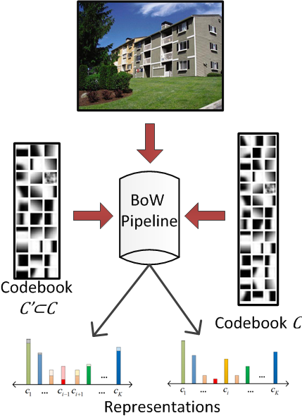
Figure 1: To analyze the classification performance of possible subsets ${C^{\prime}\subset C}$ of visual words requires instantiating the BoW pipeline to compute the new representation of an entire corpus with respect to ${C^{\prime}}$. This is computationally very demanding, since it requires re-coding and re-pooling of all items in the corpus with respect to ${C^{\prime}}$.

1 Introduction

The Bag-of-Words approach (BoW) is now a standard image representation scheme employed in the computer vision community. A quick search on Google Scholar shows that approximately $20\%$ of the papers in the recent proceedings of the top three vision conferences contain the term “bag of words”. The BoW pipeline (illustrated in Fig. 1) comprises: extracting features, coding features with respect to a learned codebook, and pooling coded features to obtain the final representation of an image [1, 9]. The computational cost of the BoW pipeline is usually dominated by the coding step, i.e., computing coding vectors corresponding to the extracted local features of an image. Coding is especially a bottleneck when the local features are sampled densely and the size of the codebook is kept large. The dimensionality of the representation vector is usually a function of the cardinality of the codebook, and larger codebooks generally result in larger representation vectors and, thus, they require more storage. Moreover, larger codebooks can in fact lead to degraded classification or retrieval accuracy, due to the curse of dimensionality [6].

Codeword selection methods that find a subset of the vocabulary that is most discriminative for a given task have been proposed to alleviate the abovementioned problems [19, 8, 18, 16, 11]. Many selection methods are adapted from the document retrieval domain, which uses criteria such as the term frequency, information gain, or ${\chi}^{2}$ measure to select terms to prune from the initial vocabulary with minimal sacrifice in retrieval/categorization accuracy [21].

However, there is a caveat: to the best of our knowledge all previous codeword selection schemes still require computing coding vectors with respect to the initial, larger vocabulary. Therefore, the prior work on this problem does not truly reduce the size of the codebook in the sense that codewords deemed unworthy are not discarded. Instead, previous methods generally use the full codebook to obtain an initial image representation, and then the reduced-dimensionality representation is computed from that. Consequently, if the initial vocabulary size is large then the computational cost of coding may still result in inefficiencies, especially on low performance platforms. Moreover this large vocabulary must still be retained in the system.

In order to truly reduce the size of the codebook, one must analyze the image representations computed under different subsets ${C^{\prime}}$ of the visual words from the initial, larger codebook ${C}$ and select the best subset with respect to some given criteria. One major drawback in this alternative scheme is the huge computational cost, since for each different subset of codewords ${C^{\prime}}$ the BoW process must be instantiated in order to compute the new representations of an entire corpus.

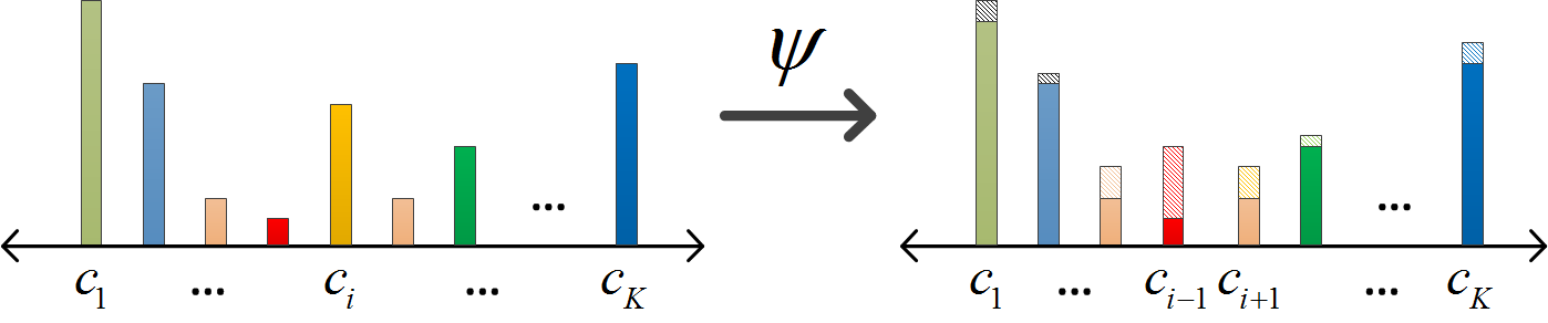
Figure 2: When a visual word is omitted from the codebook, the representation vector (a histogram in this figure) is altered. In the proposed formulation, when a visual word is omitted $\psi$ is used to approximate the feature vector, thereby avoiding re-coding and re-pooling.

In this paper, we provide a unique perspective on the BoW process that will allow us to compute the representations under subsets ${C^{\prime}}$ very efficiently. Specifically, given an image representation vector computed with respect to a vocabulary ${C}$, we formulate a technique that can approximately infer the vector representation when a visual word is pruned from the vocabulary (illustrated in Fig. 2). In this paper, we focus on assignment-based coding techniques, i.e., hard and soft (kernel) coding with average pooling, which together have wide adoption and are the basis for many other coding schemes in the literature [23, 13, 7]. Our observation is that, assuming the initial codebook construction step partitions the feature space allowing a generative model interpretation, one could use this structure to infer the alteration of a representation vector without the need for re-coding or re-pooling.

Based on our formulation, we demonstrate an efficient simulated annealing algorithm for decreasing the size of a codebook with respect to a classification task. We evaluate our algorithm on the 15-Scenes [9] and Caltech-10 [2] benchmarks, and compare against two codeword selection solutions [4, 19]. We demonstrate at least competitive classification performance at the gain of a decreased computational complexity in codebook pruning and decreased space complexity because we do not need to retain the initial codebook for use in coding new images. In summary, we make two primary contributions:

1. A method for inferring the representation vector for the hard and soft (kernel) coding methods, without doing coding or pooling in a BoW model when visual words are pruned from a vocabulary,

2. A codeword pruning scheme that eliminates the burden of considering the initial vocabulary in coding new images with respect to a reduced codebook.

The outline of the paper is as follows. In Section 2, we review related work. In Section 3, we describe our formulation. In Section 4, we present the experimental setup and discuss about the results. Finally, in Section 5 we provide concluding remarks and future work.

2 Related Work

Among many coding techniques in the literature we list only the most relevant and notable ones. These are methods like hard and soft (kernel) coding in which the features of an image are encoded by assigning them to the codebook entities [14, 5], methods that solve an optimization problem to determine the coding parameters [20, 15], and techniques that consider characterizing an image with the gradient information derived from a probability density function that models the generation process of the local features [13]. The computational cost is dominated by the coding step in these works, especially when the local features are sampled densely and the size of the codebook is large.

Borrowing ideas from the document retrieval domain [21], traditional codeword selection methods use criteria such as the term frequency, ${\chi}^{2}$ statistic, mutual information and learned SVM weights to select the most discriminative codewords [19, 8]. Winn and Minka [18] propose to merge visual words/textons with respect to a probabilistic measure defined on the altered representations. Doing so they aim to find dimensions in the original representation to merge that presumably correspond to the same textures but are captured under different lighting or viewing angles. Similarly, Fulkerson et al. [4] merges pairs of visual words based on a mutual information measure. Wang [16] employs a boosting mechanism where each weak classifier is associated with a codeword and selection of weak classifiers in the procedure naturally results in the selection of the most discriminative codewords. Zhang, et al. [22] considers an unsupervised scheme in which the visual words are selected by constructing a ridge regression formulation.

Note that in all of these works, the requirement of computing the coding vectors with respect to the initial codebook still remains.

$\mathbf{x}$	local feature extracted from a local patch
$\mathbf{V}$	vocabulary (codebook)
$K$	cardinality of the vocabulary
$d$	dimensionality of $\mathbf{x}$
$\mathbf{c}$	codeword/visualword/basis of vocabulary
${\mathbf{h}}_{i}$	coding vector of local feature ${\mathbf{x}}_{i}$
$\mathcal{F}$	space of the coding vector
${\mathbf{f}}_{i}$	representation vector after pooling coding vectors ${{\mathbf{h}}_{i}}$
$\underline{{\mathbf{h}}_{i}}$	coding vector after pruning a basis from codebook
$\underline{\mathcal{F}}$	dimensionality reduced coding vector space
$\underline{{\mathbf{f}}_{i}}$	representation vector after pooling coding vectors $\underline{{\mathbf{h}}_{i}}$
$I$	set of visual word indices in the codebook
$\mathcal{R}$	a particular region or voronoi cell in the codebook space
$\underline{\mathcal{R}}$	a particular region or voronoi cell in the codebook space when a basis is pruned
$y$	a class/category
$N$	Number of local features in an image

Table 1: Notation.

3 Formulation

3.1 Mathematical Background

The basic idea behind the Bag-of-Words (BoW) model is to describe an image with a statistical measure based on the codebook entities, e.g. a histogram describing the frequency of visual words found in the image. The central component in this model is the codebook, which is traditionally constructed by quantizing local descriptors (e.g. SIFT) extracted from a set of training images. Consequently, to compute a representation of an image, the BoW process first determines the coding coefficients of all of the extracted local features from the image. This step involves evaluating the assignment values of the local features to the codebook entities. Finally, the coefficients are pooled to obtain the final representation.

Before we proceed let us give a brief overview of these coding techniques, which will help us establish the mathematical framework and notation of the discussion.

Formally, let $\mathbf{x}\in{{\mathbb{R}}^{d}}$ describe a feature vector extracted from a local patch in an image where $d$ is the dimensionality. Let $\mathbf{V}=\{{{\mathbf{c}}_{j}}\in{{\mathbb{R}}^{d}}\}_{j=1}^{K}$ be a codebook. The likelihood function $p(\mathbf{x}|\mathbf{c})$ then expresses the distribution of the local feature vector $\mathbf{x}$ given the visual word $\mathbf{c}$. Let ${{\mathbf{h}}_{i}}\in\mathcal{F}$ be the coding coefficient vector of ${{\mathbf{x}}_{i}}$ in which a traditional BoW scheme $\mathcal{F}$ has the dimensionality equal to the cardinality of the codebook, $|\mathbf{V}|$ ($\mathcal{F}\triangleq{{\mathbb{R}}^{|\mathbf{V}|}}$). ${{h}_{ik}}$ describes the coding coefficient of ${\mathbf{x}_{i}}$ with respect to visual word ${{\mathbf{c}}_{k}}$.

Hard coding can then be defined as

$${{h}_{ik}}=\left\{\begin{matrix}1~{}~{}~{}~{}~{}~{}~{}~{}p\left({{\mathbf{c}}_{k}}|\mathbf{{x}}_{i}\right)>p\left({{\mathbf{c}}_{j}}|\mathbf{{x}}_{i}\right)~{}~{}~{}\forall j\neq k\\ 0~{}~{}~{}~{}~{}~{}~{}~{}~{}~{}~{}~{}~{}~{}~{}~{}~{}~{}~{}~{}~{}~{}~{}otherwise~{}~{}~{}~{}~{}~{}~{}~{}~{}~{}~{}~{}~{}~{}~{}~{}\\ \end{matrix}\right.$$ (1)

where $p\left({{\mathbf{c}}_{k}}|\mathbf{x}_{i}\right)$ is the posterior probability of a ${{\mathbf{x}}_{i}}$ belonging to visual word ${{\mathbf{c}}_{k}}$. With $p\left(\mathbf{x}|{\mathbf{c}}_{k}\right)\sim N({\mu}_{k},{{\sigma}^{2}}I)$ and equal priors $p({\mathbf{c}}_{k})$, the condition $p\left({{\mathbf{c}}_{k}}|{{\mathbf{x}}_{i}}\right)>p\left({{\mathbf{c}}_{j}}|{{\mathbf{x}}_{i}}\right)~{}\forall j\neq k$ becomes $k=\underset{j=1,\ldots,K}{\mathop{\arg\min}}\,\|{{\mathbf{x}}_{i}}-{{\mathbf{c}}_{j}}\|_{2}$. This assumption is considered when the codebook generation step involves $K$-means clustering.

Similarly, soft coding can be defined as the posterior probability of assigning a local feature ${{\mathbf{x}}_{i}}$ to visual word ${{\mathbf{c}}_{k}}$,

$${{h}_{ik}}=p\left({{\mathbf{c}}_{k}}|{{\mathbf{x}}_{i}}\right)=\frac{1}{Z}\exp(-\beta\delta({{\mathbf{x}}_{i}},{{\mathbf{c}}_{k}}))$$ (2)

where $Z=\underset{j}{\mathop{\sum}}\,\exp(-\beta\delta({{\mathbf{x}}_{i}},{{\mathbf{c}}_{j}}))~{}$is the normalization factor, $\beta$ is a parameter controlling the degree of the assignment and $\delta$ is a distance function. Finally, to obtain the BoW representation vector of the image for hard and soft coding, we consider average pooling as $\mathbf{f}=\frac{1}{N}\underset{i=1}{\overset{N}{\mathop{\sum}}}\,{{\mathbf{h}}_{i}}$.

In the next section we will describe our method to compute the final image representation without having to go through the usual coding and pooling steps when pruning a codeword or a subset of codewords from the codebook.

3.2 Methodology

Before we proceed let us define the necessary notation. After we prune a subset of visual words from an initial codebook, the resulting new coding coefficient and representation will be described by $\underline{\mathbf{h}},\underline{\mathbf{f}}\in\underline{\mathcal{F}}$, respectively. If the local features are assumed to be known, these vectors can be exactly computed; thus, they will represent the deterministic solution of the BoW process. Otherwise we will regard them as random variables. This difference will be apparent or noted in the paper. See Table 1 for complete notation.

3.2.1 Hard-coding and average pooling

After pruning a subset of visual words from the codebook, how can we infer the representation of an image with respect to the remaining codebook entities without re-coding and re-pooling? Our observation to this is that, assuming the codebook partitions the feature space with an underlying generative model, one can use this structure to infer the alteration of the representation vector without having to redo coding or pooling. To elaborate, consider the example Voronoi tesselation after quantizing a set of local features with $K$-means in Fig. 2. The Voronoi centers describe the visual words in this diagram and the Voronoi cells denote the regions consisting of local features closer (with respect to the Euclidean norm in this case) to that visual word than to any other. As a result, in hard coding, a local feature is assigned with respect to which Voronoi cell it falls into.

Assume we prune codeword ${{\mathbf{c}}_{l}}$, the neighboring cells will then invade its region and the local features previously assigned to ${{\mathbf{c}}_{l}}$ will be distributed among them. Consider another visual word $\mathbf{c}_{k}$, the probability that a local feature previously in region of $\mathbf{c}_{l}$ gets assigned to $\mathbf{c}_{k}$ can be approximated as a function of the location of the local feature and the proportion of volume ${{\mathbf{c}}_{k}}$ that ‘invades’ after ${{\mathbf{c}}_{l}}$ is pruned. Formally this probability can be stated as

$${\Lambda}_{k,l}=\frac{1}{Z^{\prime}}\underset{\underline{\mathcal{R}}({\mathbf{c}}_{k})\mathop{\cap}\mathcal{R}({{\mathbf{c}}_{l}})}{\overset{{}}{\mathop{\int}}}\,p(\mathbf{x}|{{\mathbf{c}}_{l}})d\mathbf{x}$$ (3)

where $Z^{\prime}$ is a normalization factor described as $Z^{\prime}=\underset{{{\mathbf{c}}_{k}}\in N({{\mathbf{c}}_{l}})}{\mathop{\sum}}\,\underset{\underline{\mathcal{R}}({\mathbf{c}}_{k})\mathop{\cap}\mathcal{R}({{\mathbf{c}}_{l}})}{\overset{{}}{\mathop{\int}}}\,p(\mathbf{x}|{{\mathbf{c}}_{l}})d\mathbf{x}$ in which $\mathcal{R}({\mathbf{c}}_{k})$ and $\underline{\mathcal{R}}({\mathbf{c}}_{k})$ denote the regions in the descriptor space where $p\left(\mathbf{x}|{{\mathbf{c}}_{k}}\right)>p\left(\mathbf{x}|{{\mathbf{c}}_{j}}\right)~{}\forall j\neq k$ before and after removing visual word ${\mathbf{c}}_{l}$, $\mathop{\cap}$ describes the intersection of the regions and $N({\mathbf{c}}_{l})$ is the set of visual words for which their regions are incident to $\mathcal{R}({\mathbf{c}}_{l})$.

After omitting ${\mathbf{c}}_{l}$, let the new image representation obtained through the usual BoW process be $\underline{\mathbf{f}}=\frac{1}{N}\underset{i=1}{\overset{N}{\mathop{\sum}}}\,{\underline{{\mathbf{h}}_{i}}}$ where $\underline{{\mathbf{h}}_{i}},\underline{{\mathbf{f}}}\in\underline{\mathcal{F}}$ and let $\mathcal{I}=\{1,..,K\}$ denote the visual word indices in the initial codebook. We then specify a mapping ${\Psi}:\mathcal{F}\times I\to\underline{\mathcal{F}}$ to approximate $\underline{\mathbf{f}}$. This mapping function is described as

$${{\psi}_{k}}\left(\mathbf{f},l\right)=\left\{\begin{matrix}{{f}_{k}}+{\Lambda}_{k,l}\times{{f}_{l}}~{}~{}~{}~{}~{}~{}~{}~{}~{}{{\mathbf{c}}_{k}}\in N\left({{\mathbf{c}}_{l}}\right),~{}k<l\\ {{f}_{k}}~{}~{}~{}~{}~{}~{}~{}~{}~{}~{}~{}~{}~{}~{}~{}~{}~{}~{}~{}~{}~{}~{}~{}~{}~{}~{}~{}{{\mathbf{c}}_{k}}\notin N\left({{\mathbf{c}}_{l}}\right),~{}k<l\\ \end{matrix}\right.$$ (4)

where $l$ denotes the index of the omitted visual word in the codebook. If we consider the conditional densities to be Gaussian distributions, $p\left(\mathbf{x}|{\mathbf{c}}_{k}\right)\sim{\ }N({{\mu}_{k}},{{\Sigma}_{k}})$, then the regions correspond to the Voronoi cells under the decomposition of a Mahalanobis metric space.

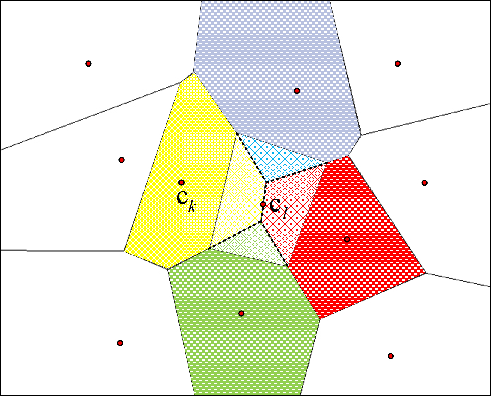
Figure 3: Voronoi tesselation of the feature space describing the quantization of a set of local descriptors. The Voronoi centers denote the visual words and Voronoi cells denote the regions consisting of local descriptors closer to that visual word than to any other.

Proposition 1 (Hard-coding and average pooling) Under hard coding and average pooling, when local features are i.i.d sampled from $p(\mathbf{x}|{{\mathbf{c}}})$, then $\mathbb{E}[\underline{\mathbf{f}}]=\Psi\left(\mathbf{f},l\right)$.

Proof: Let $\underline{{f}_{k}}=\frac{1}{N}\underset{i=1}{\overset{N}{\mathop{\sum}}}\,\underline{{h}_{ik}}=\frac{1}{N}[\underset{i\in{{S}_{1}}}{\mathop{\sum}}\,\underline{{h}_{ik}}+\underset{i\in{{S}_{2}}}{\mathop{\sum}}\,\underline{{h}_{ik}}]$ where we partition the local features into two disjoint sets ${{S}_{1}}$ and ${{S}_{2}}$, where ${{S}_{1}}$ contains the indices of the local features that are $p\left({{\mathbf{c}}_{l}}\text{ }\!\!|\!\!\text{ }{{\mathbf{x}}_{i}}\right)>p\left({{\mathbf{c}}_{k}}\text{ }\!\!|\!\!\text{ }{{\mathbf{x}}_{i}}\right)~{}\forall k\neq l$ and ${{S}_{2}}$ contains rest of the indices. Thus the coding coefficients $\underline{{h}_{ik}}~{}(i\in{{S}_{1}})$ are Bernoulli random variables while $\underline{{h}_{ik}}~{}(i\in{{S}_{2}})$ are deterministic. We see that $\frac{1}{N}\underset{i\in{{S}_{2}}}{\mathop{\sum}}\,\underline{{h}_{ik}}=\frac{1}{N}\underset{i=1}{\overset{N}{\mathop{\sum}}}\,{{h}_{ik}}$ and thus ${\mathbb{E}}[\frac{1}{N}\underset{i\in{{S}_{2}}}{\mathop{\sum}}\,\underline{{h}_{ik}}]={{f}_{k}}$.

If ${{\mathbf{c}}_{k}}\in N({{\mathbf{c}}_{l}})$ then $\Pr[\underline{{h}_{ik}}=1]={\Lambda}_{k,l}~{}(i\in{{S}_{1}})$ where ${\Lambda}_{k,l}$ is defined as above. Consequently,

$$\begin{split}\mathbb{E}[\underline{{f}_{k}}]&=\mathbb{E}\left[\frac{1}{N}[\underset{i\in{{S}_{1}}}{\mathop{\sum}}\,\underline{{h}_{ik}}+\underset{i\in{{S}_{2}}}{\mathop{\sum}}\,\underline{{h}_{ik}}]\right]\\ &=\frac{1}{N}\mathbb{E}[\underset{i\in{{S}_{1}}}{\mathop{\sum}}\,\underline{{h}_{ik}}]+{{f}_{k}}\\ &=\frac{{\Lambda}_{k,l}\times|{{S}_{1}}|}{N}+{{f}_{k}}\end{split}$$ (5)

where $\frac{|{{S}_{1}}|}{N}={{f}_{l}}$ and $\mathbb{E}[\underset{i\in{{S}_{1}}}{\mathop{\sum}}\,\underline{{h}_{ik}}]$ is the expected value of sum of Bernoullis, a Binomial distribution. Note also that $\text{var}\left(\underline{{f}_{k}}\right)=\frac{\left|{{S}_{1}}\right|{{\Lambda}_{k,l}}\left(1-{{\Lambda}_{k,l}}\right)}{{{N}^{2}}}$.

If ${{\mathbf{c}}_{k}}\notin N({{\mathbf{c}}_{l}})$ then $\Pr\left[\underline{{h}_{ik}}=1\right]=0~{}(i\in{{S}_{1}})$ since $\mathcal{R}\left({{\mathbf{c}}_{k}}\right)\mathop{\cap}\mathcal{R}\left({{\mathbf{c}}_{l}}\right)=\emptyset$. This is true because if the pruned visual words ${{\mathbf{c}}_{l}}$ and ${{\mathbf{c}}_{k}}$ are not neighbours in the Voronoi tessellated feature space then after pruning ${{\mathbf{c}}_{l}}$, $\exists j$ such that $p\left({{\mathbf{c}}_{j}}\text{ }\!\!|\!\!\text{ }{{\mathbf{x}}_{i}}\right)>p({{\mathbf{c}}_{k}}|{{\mathbf{x}}_{i}})$. Then $\mathbb{E}[\underset{i\in{{S}_{1}}}{\mathop{\sum}}\,\underline{{h}_{ik}}]=0$, and thus $\mathbb{E}\left[\underline{{f}_{k}}\right]={f}_{k}$. Finally, we see that $\mathbb{E}\left[\underline{{f}_{k}}\right]={\psi}_{k}\left(\mathbf{f},l\right)$.

$\square$

The above proposition is important, as it states that given an image, with hard coding and average pooling, if the local features are sampled densely enough (or the number of local features is high) Eq. 4 allows one to compute the representation of an image without having to do re-coding and pooling, which is a significant advantage since it bypasses the computationally expensive nearest neighbour searches.

If we consider $p\left(\mathbf{x}|{\mathbf{c}}_{k}\right)\sim{\ }N({{\mu}_{k}},{{\sigma}^{2}}I)$ in which the codebook corresponds to the Voronoi tesselation under the Euclidean metric, the complexity of computing the Voronoi diagram in $d$-dimensions is computationally prohibitive [3]. In the general case, we propose to use a heuristic, as explained next, which uses nearest neighbor information of a visual word to approximate $\underline{\mathcal{R}}({{\mathbf{c}}_{k}})\mathop{\cap}\mathcal{R}({{\mathbf{c}}_{l}})$ in Eq. 3.

Heuristic for hard-coding If the dimensionality of the feature space is high, constructing the Voronoi diagram to evaluate Eq. 3 is generally intractable . In order to also avoid the integration in high dimensions of Eq. 3 we only use the neighborhood information of the pruned visual word to approximate ${\Lambda}_{k,l}$. This neighborhood information is with respect to a metric, not the neighbors in the Voronoi diagram of the pruned visual word ${{\mathbf{c}}_{l}}$ $(N({{\mathbf{c}}_{l}}))$. We show that this simplification shows good performance results.

Formally, we revise Eq. 4 to incorporate this heuristic. Assume the set ${{N}_{\delta}}({{\mathbf{c}}_{l}})$ contains the nearest neighbors of ${{\mathbf{c}}_{l}}$ in the codebook space based on some distance function $\delta:\mathcal{X}\times\mathcal{X}\to\mathbb{R}$. For example, if the initial codebook has been constructed by $K$-means this distance function would be the ${{l}_{2}}-$norm. The cardinality of this set is a user specified parameter. Consequently, Eq. 4 is revised as

$${\psi}_{k}\left(\mathbf{f},l\right)=\left\{\begin{matrix}{{f}_{k}}+\frac{{{f}_{l}}}{|{{N}_{\delta}}({{\mathbf{c}}_{l}})|}~{}~{}~{}~{}~{}~{}~{}~{}{{\mathbf{c}}_{k}}\in{{N}_{\delta}}\left({{\mathbf{c}}_{l}}\right),~{}k<l\\ {{f}_{k}}~{}~{}~{}~{}~{}~{}~{}~{}~{}~{}~{}~{}~{}~{}~{}~{}~{}~{}~{}~{}~{}~{}~{}~{}~{}~{}{{\mathbf{c}}_{k}}\notin{{N}_{\delta}}\left({{\mathbf{c}}_{l}}\right),~{}k<l\\ \end{matrix}\right.$$ (6)

3.2.2 Soft-coding and average pooling

In this section we will examine another popular coding scheme used in the literature. Compared to hard coding, soft coding assigns a local feature to each codebook entity and computes its degree of membership to them. When a visual word is pruned, the new representation vector can be computed exactly if we maintain the initial coding information of the local features. Formally, let $\mathcal{I}=\{1,..,K\}$ again denote the visual word indices in the initial codebook. With soft-coding and average pooling schemes, assume we maintain the initial coding vectors $\mathbf{H}=[{{h}_{ik}}]$ where ${{h}_{ik}}=\exp(-\beta\delta\left({{\mathbf{x}}_{i}},{{\mathbf{c}}_{k}}\right))/\underset{j}{\mathop{\sum}}\,\exp(-\beta\delta\left({{\mathbf{x}}_{i}},{{\mathbf{c}}_{j}}\right))$. Then we describe the new feature representation as

$${{\upsilon}_{k}}\left(\mathbf{H},l\right)=\frac{1}{N}\underset{i=1}{\overset{N}{\mathop{\sum}}}\,[\frac{{{h}_{ik}}}{\mathop{\sum}_{k=1,k\notin S}^{K}{{h}_{ik}}}]$$ (7)

where $\mathcal{S}\subset\mathcal{I}$ contains the indices of the visual words to be pruned. Note that $\underline{{f}_{k}}=\frac{1}{N}\underset{i=1}{\overset{N}{\mathop{\sum}}}\,\underline{{h}_{ik}}$ where $\underline{{h}_{ik}}=\exp\left(-\beta\delta\left({{\mathbf{x}}_{i}},{{\mathbf{c}}_{k}}\right)\right)/\underset{k=1,k\notin S}{\overset{K}{\mathop{\sum}}}\,\exp(-\beta\delta({{\mathbf{x}}_{i}},{{\mathbf{c}}_{k}}))$ represents the deterministic (exact) solution of the BoW model when the subset of visual words are pruned.

Claim 2 (Soft-coding and average pooling) Under such schemes, $\boldsymbol{\upsilon}=\underline{\mathbf{f}}.$

Proof: It is easy to verify that

$$\begin{split}{{v}_{k}}=\frac{1}{N}\underset{i=1}{\overset{N}{\mathop{\sum}}}\,\frac{{{h}_{ik}}}{\left[\mathop{\sum}_{k=1,k\notin S}^{K}{{h}_{ik}}\right]}&=\frac{\frac{\exp\left(-\beta\delta\left({{\mathbf{x}}_{i}},{{\mathbf{c}}_{k}}\right)\right)}{\mathop{\sum}_{k=1}^{K}\exp\left(-\beta\delta\left({{\mathbf{x}}_{i}},{{\mathbf{c}}_{k}}\right)\right)}}{\frac{\mathop{\sum}_{k=1,k\notin S}^{K}\exp\left(-\beta\delta\left({{\mathbf{x}}_{i}},{{\mathbf{c}}_{k}}\right)\right)}{\mathop{\sum}_{k=1}^{K}\exp\left(-\beta\delta\left({{\mathbf{x}}_{i}},{{\mathbf{c}}_{k}}\right)\right)}}\\ &=\underline{{f}_{k}}\end{split}$$ (8)

$\square$

Thus, maintaining the initial coding vectors allows us to exactly compute the new representation vector.

3.3 Example Codeword Selection Application

We now describe an example codeword selection scheme, where a subset of codewords is selected to maximize a given objective function via a simulated annealing process. The techniques developed in the previous section allow us to bypass the computationally expensive re-coding step (and also re-pooling for hard coding), which allows us to compute the altered representations under various subsets of visual words very efficiently.

Data: Initial codebook $V=\{{{\mathbf{c}}_{1}},{{\mathbf{c}}_{2}},\ldots,{{\mathbf{c}}_{k}}\}$, initial representation matrix of the data ${\Pi}^{0}$, $tmax,\lambda$

begin

       ${\mathcal{T}}^{0}\leftarrow$ initial subset of visual words (initial state);

       ${e}^{0}\leftarrow$ initial energy;

       $t\leftarrow 0$ ;

       while t $<$ tmax do

             compute altered feature representation according to Eq. 6 or Eq. 7;

             $\underline{\Pi^{t}}\leftarrow get\_feature\_representations(\Pi^{t-1},{\mathcal{T}}^{t})$;

             assuming a distribution for each bin (visual word ${v}_{k}$), estimate its parameters;

             $\{\hat{\theta}\}_{i=1}^{|{\mathcal{T}}^{t}|}\leftarrow maximum\_likelihood(\underline{\Pi^{t}})$;

             calculate score according to Eq. 9;

             ${e}^{t}\leftarrow maximum\_relevance(\{\hat{\theta}\}_{i=1}^{|{\mathcal{T}}^{t}|},\underline{\Pi^{t}})$;

             $\Delta e={e}^{t}-{e}^{t-1}$;

             $\Pr\left[Accept\right]\leftarrow{{e}^{\frac{\Delta e}{{{\lambda}^{t}}}}}$;

             if $\Pr\left[Accept\right]<random(0,1)$ then /* Reject, ${\mathcal{T}}^{0}$ always accepted */

                   ${e}^{t}\leftarrow{e}^{t-1}$;

                   ${\mathcal{T}}^{t}\leftarrow{\mathcal{T}}^{t-1}$;

                  

             end if

            get neighbour state;

             ${\mathcal{T}}^{t+1}\leftarrow neighbour({\mathcal{T}}^{t})$;

             $t\leftarrow t+1$;

            

       end while

      

end

Result: ${\mathcal{T}}^{t}$

Algorithm 1 Simulated annealing based codeword selection.

There are many scoring functions, such as error probability, inter-class distance, etc., to employ in a standard feature selection technique. After obtaining the final representation vectors (i.e. histogram) of images in the dataset, $\underline{\mathbf{{f}}}$, we consider the maximum relevancy score [12] defined as

$$D\left(\mathcal{T},y\right)=\frac{1}{|\mathcal{T}|}\underset{\underline{{{f}_{k}}}\in\mathcal{T}}{\mathop{\sum}}\,I(\underline{{{f}_{k}}};y)$$ (9)

where $\mathcal{T}$ is the set of indices of the visual words used to infer the representation vector (i.e., the set $\mathcal{I}\backslash\mathcal{S}$) and $I\left(\underline{{{f}_{k}}};{y}\right)$ is the mutual information defined as a function of the (differential) entropy with respect to the ${k}^{th}$ bin of $\underline{{f}}$ and class $y$:

$$I\left(\underline{{{f}_{k}}};y\right)=h\left(\underline{{{f}_{k}}}\right)-\mathop{\int}p\left(y\right)h(\underline{{{f}_{k}}}|y)dy.$$ (10)

We summarize the feature selection procedure in Algorithm 1 in which we assume $\underline{{{f}_{k}}}\sim\text{Beta}(\alpha,\beta)$ where the parameters are estimated via maximum likelihood given the feature representation vectors of the data.

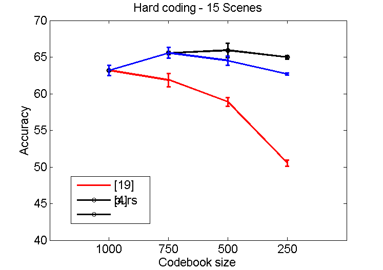
(a) Hard coding - 15 Scenes - 1000

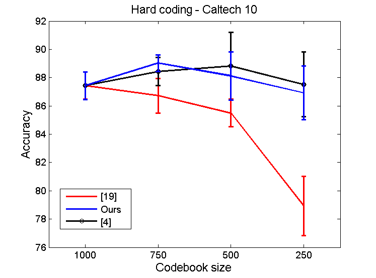
(b) Hard coding - Caltech 10 - 1000

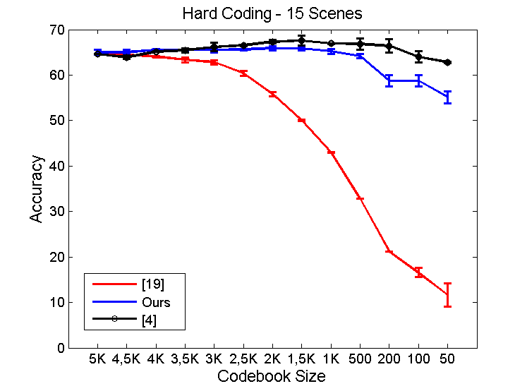
(c) Hard coding - 15 Scenes - 5000

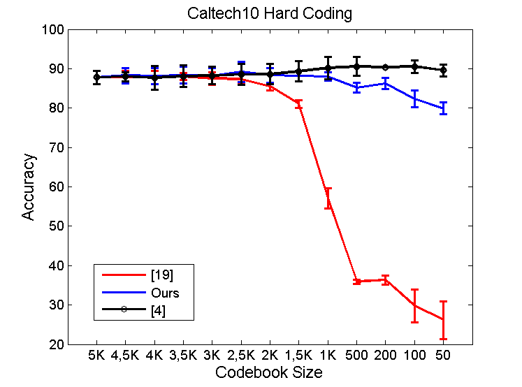
(d) Hard coding - Caltech 10 - 5000

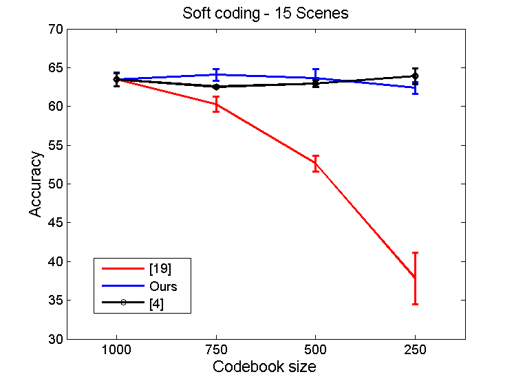
(e) Soft coding - 15 Scenes - 1000

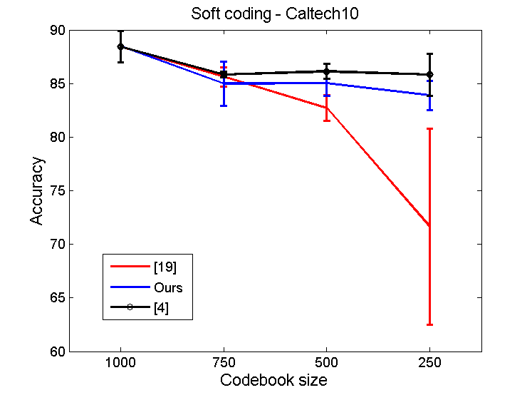
(f) Soft coding - Caltech 10 - 1000

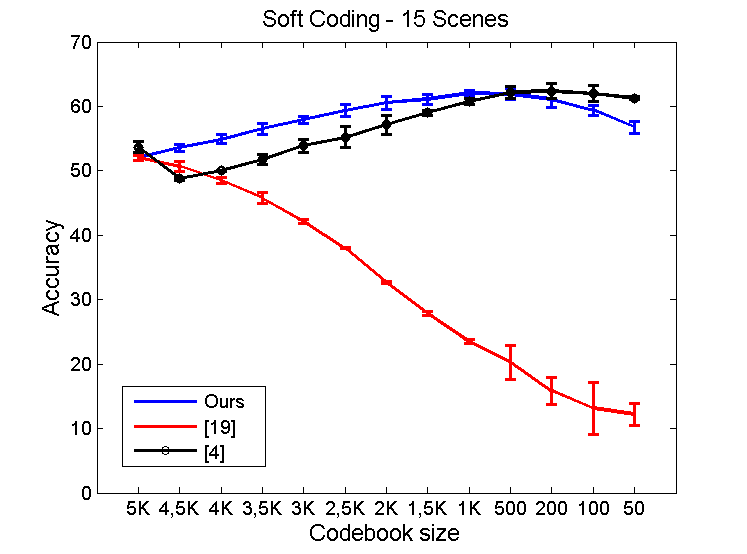
(g) Soft coding - 15 Scenes - 5000

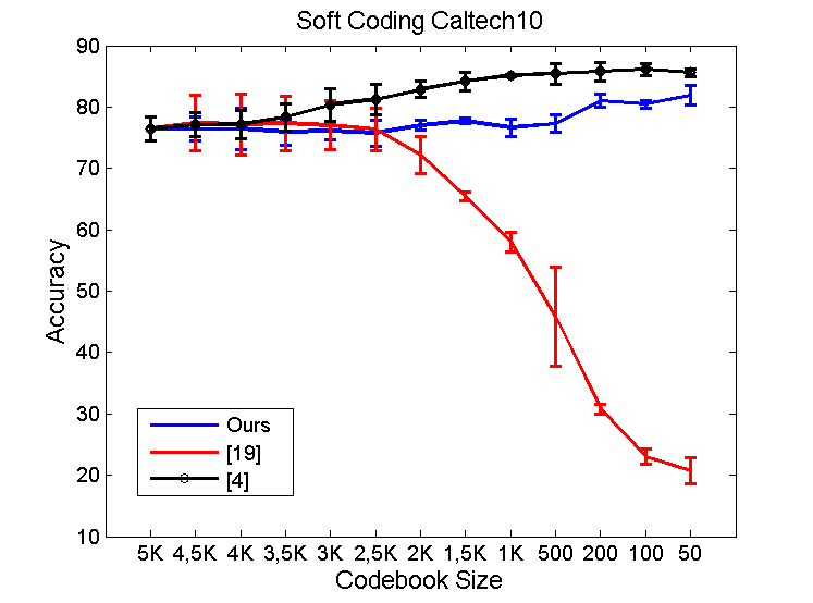
(h) Soft coding - Caltech 10 - 5000

Figure 4: Comparison of our method with respect to a baseline. The vertical axes in the sub-figures denote the average classification accuracy of the categories while the horizontal axes denote the codebook sizes. The caption ’Soft coding - Caltech 10 - 1000’ denotes the soft coding case performed on the Caltech 10 dataset with an initial codebook size of 1000.

4 Experiments

In our experiments, our focus is on not to achieve state-of-the-art classification results but to demonstrate that the techniques we developed can be used in a codeword selection problem where the task is to obtain a compact codebook. We compare our method against [19, 4], where similar entropy-based measures are used for characterizing the discriminative power of the visual words. We hope to observe little sacrifice in classification performance vs. these techniques, while avoiding the expense of re-coding representation vectors with respect to an initial codebook.

Two image classification benchmark datasets are used in our evaluation: 15-Scenes and Caltech-10. For both datasets, each image is first resized such that neither its height nor width exceeds 300 pixels. Densely sampled SIFT [10] descriptors on a single scale of $16\times 16$ patches with step size equal to 8 pixels are extracted. We use $K$-means clustering to create two visual vocabularies for each dataset, where the number of clusters is set to 1000 and 5000. The number of neighbors that determines the cardinality of $|{{N}_{\delta}}\left({{\mathbf{c}}_{l}}\right)|$ is set to be 5. $\lambda$ is set to be $0.9$ and $tmax$ is set to $100$ and $500$ for the hard coding and soft coding cases, respectively. The neighbor state in Alg. 1 alters set $T$ by replacing a subset with their corresponding nearest neighbors in codebook space. The size of this subset is chosen to be 10. Finally all experiments are conducted 5 times over random subsets of images.

For 15-Scenes, 50 images are used for generating a codebook and an additional 50 images are used for determining which visual word to prune based on Alg. 1. Once the visual words are pruned, the same 50 images are used for training a linear SVM. Hence, 100 images are used in total for training, and the remaining images are used for testing.

Our second benchmark contains the largest 10 categories (except for BACKGROUND_Google category and Faces_easy) from the Caltech-101 dataset. 25 images per category are used to train a codebook and 25 are used to select visual words to prune based on Alg. 1. Once the visual words are pruned, the same 25 images are used for training a linear SVM. The remaining images are used for testing.

4.1 Discussion

Fig. 4 shows our results. The vertical axes in the sub-figures denote the average classification accuracy of the categories while the horizontal axes denote the codebook sizes. First of all we see that the approach of [19] shows inferior performance compared to [4] and our technique. This is especially apparent when the initial codebook size is large. After a certain number of visual word pruning steps, the classification performance degrades severely. This suggests that removing the bins of the image representation corresponding to the pruned set of visual words also reduces the discriminative power of the representation. On the other hand, the performance of [4] shows that merging the bins instead of completely discarding them can improve the classification performance. This may be due to the fact that certain visual words correspond to the same texture but due to different lighting conditions or other effects it may have been represented by multiple words. Hence, merging the bins will not reduce the discriminative ability but enhance it while also eliminating the redundancy in the codebook.

Our technique shows competitive performance with [4]. Notice that for both techniques the curve of the accuracy values across different sizes of the codebook demonstrate that under certain tasks the codebook is overcomplete with noisy visual words. In fact in certain cases we decrease the size of the codebook by two orders of magnitude while increasing the overall accuracy. Also we see that both [4] and our technique have more impact when started with an overcomplete codebook. One other thing to notice that both hard and soft coding outperformed each other in certain cases.

However, the crucial advantage of our method is the fact that we truly reduce the size of the codebook and thus need not store it. We explore the space of subsets of visual words via the Simulated Annealing method. A disadvantage of this method is that it may require lengthy simulations to find a “good” state, i.e. the subset of visual words that is satisfactory, since the number of states to consider is very large and also the energy function is multimodal. Despite these issues, our method performs well in relatively few iterations as noted in the preceding section. Moreover, this exploration would have normally required the instantiation of the BoW process for each subset of the codebook, but our analysis alleviates this burden by approximating the image representations without doing coding and pooling.

Overall, compared to a brute-force solution of our problem, we explored the solution space (subset of visual words) without having to do re-coding and re-pooling. Compared to previous codeword reduction techniques this analysis enables us to truly reduce the codebook.

4.1.1 Complexity Analysis

Compared to previous codeword selection schemes, we reduce the time complexity by eliminating the need of re-coding with respect to the initial codebook. For example, for the Caltech 10 dataset, [4] reduces the size of the codebook by two orders of magnitude, from 5000 to 50. However, they still require doing coding with respect to the 5000 visual words to compute image representations, which is computationally inefficient if one considers thousands of images. Formally, after the codeword selection process. the complexity of coding new image representations becomes $\mathcal{O}(d|\mathcal{T}|N)$ compared to $\mathcal{O}(d|V|N)$ where $V$ denotes the initital codebook and $|\mathcal{T}|<<|V|$. Likewise we also reduce the space complexity since we do not need to store the 5000-word codebook.

As stated, for each state during the simulation, the BoW must be instantiated for an entire corpus. However, we explore the state space without having to do re-coding and re-pooling. Compared to the brute-force approach where the BoW is instantiated at every step, we analyze the reductions in complexity afforded by our formulations.

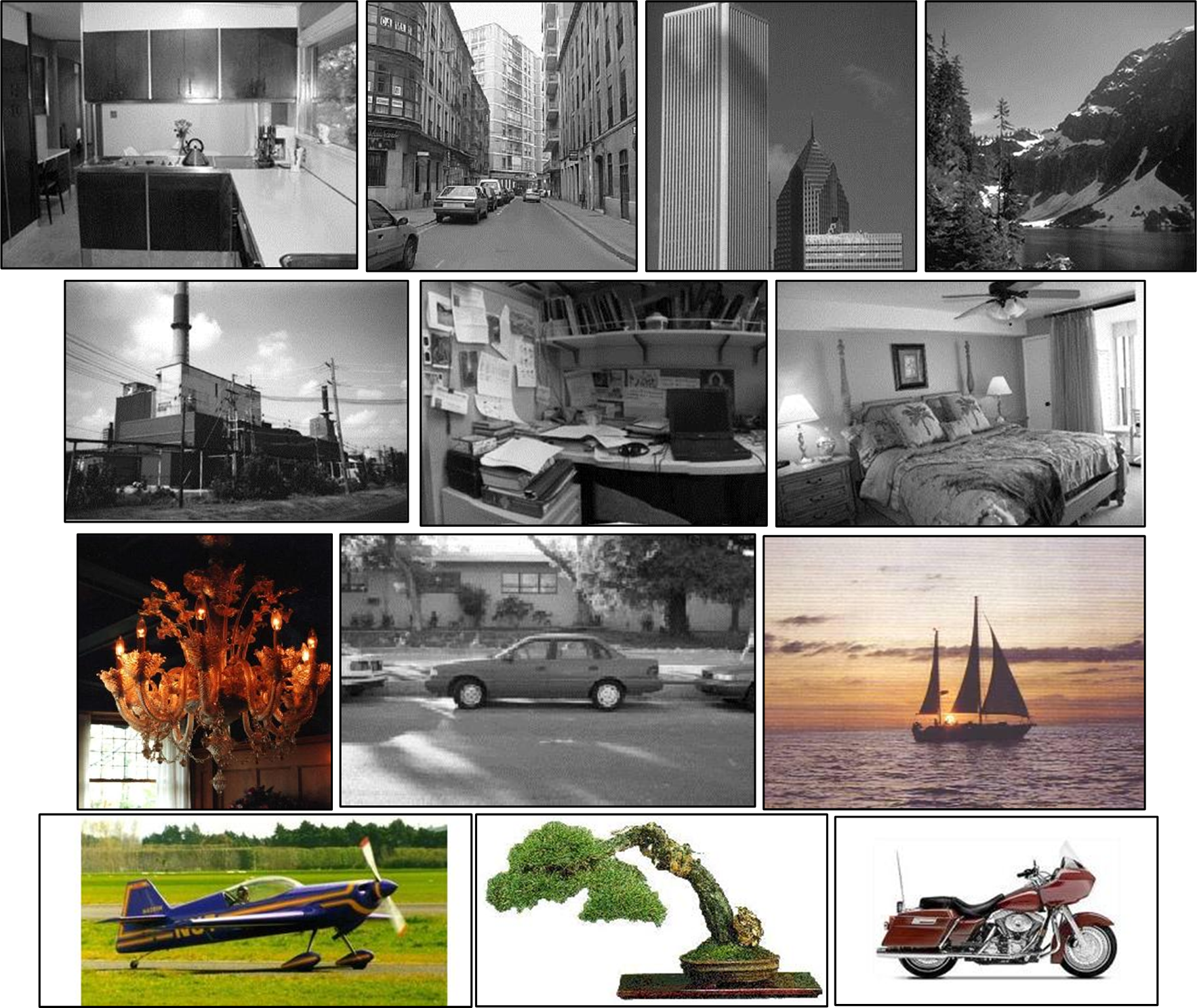
Figure 5: Example images from the Caltech 10 (top two rows) and 15 Scenes datasets (bottom two rows).

Hard-coding: Suppose we remove the set of visual words $\mathcal{S}$, instantiating the BoW pipeline to compute the new representation under the set of the remaining visual words $\mathcal{T}$ would require a nearest-neighbor search for all extracted local features. Given the fact that a naïve NN search outperforms techniques based on partitioning the feature space in high dimensions, we assumed an $\mathcal{O}(d~{}|\mathcal{T}|)$ complexity [17]. Thus, the complexity is $\mathcal{O}(d~{}|\mathcal{T}|~{}N)$ where $N$ is the number of local features with $d$ dimensionality. This coding step dominates pooling, which has complexity $\mathcal{O}(|\mathcal{T}|~{}N)$.

In contrast, our technique has $\mathcal{O}(|\mathcal{S}||{N}_{\delta}(\mathbf{c}_{l})|)$ complexity where $|{N}_{\delta}(\mathbf{c}_{l})|<<|V|$. For each deleted visual word we distribute its bin value among its $|{N}_{\delta}(\mathbf{c}_{l})|$ neighbors. This neighbor information can be computed offline.

Soft-coding: Instantiating the BoW pipeline for computing the image representation under the set of remaining visual words again requires $\mathcal{O}(d~{}|\mathcal{T}|~{}N)$. However, maintaining the initial coding matrix $\mathbf{H}$ allows us to reduce this complexity to $\mathcal{O}(N|\mathcal{T}|)$.

5 Conclusion

We formulated and analyzed a method for inferring the representation vector in an assignment based BoW model, without the need to re-code or re-pool as visual words are pruned from a vocabulary. The formulation is demonstrated in an efficient and effective simulated annealing scheme that prunes words from a codebook. Compared to similar entropy-based solutions, our algorithm demonstrates superior results to [19], and roughly comparable results to [4] but enables reduced time and space complexity for subsequent BoW representations. We expect that our basic strategy should be applicable to other assignment based BoW models, such as the super vector [23], Fisher [13] and VLAD [7] encoding methods. This will be explored in future work.

References

- [1] G. Csurka, C. R. Dance, L. Fan, J. Willamowski, and C. Bray. Visual categorization with bags of keypoints. In Workshop on Statistical Learning in Computer Vision, ECCV, 2004.
- [2] L. Fei-Fei, R. Fergus, and P. Perona. Learning generative visual models from few training examples: An incremental Bayesian approach tested on 101 object categories. CVIU, 106(1), 2007.
- [3] K. Fukuda. Frequently asked questions in polyhedral computation, Nov. 2012.
- [4] B. Fulkerson, A. Vedaldi, and S. Soatto. Localizing objects with smart dictionaries. In Proceedings of European Conference on Computer Vision, page 2008.
- [5] J. C. Gemert, J.-M. Geusebroek, C. J. Veenman, and A. W. Smeulders. Kernel codebooks for scene categorization. In Proc. ECCV, 2008.
- [6] T. Hastie, R. Tibshirani, and J. H. Friedman. The elements of statistical learning: Data mining, inference, and prediction. New York: Springer-Verlag, 2001.
- [7] H. Jegou, M. Douze, C. Schmid, and P. Perez. Aggregating local descriptors into a compact image representation. In Computer Vision and Pattern Recognition (CVPR), 2010 IEEE Conference on, pages 3304–3311, 2010.
- [8] F. Jurie and B. Triggs. Creating efficient codebooks for visual recognition. In Proc. ICCV, 2005.
- [9] S. Lazebnik, C. Schmid, and J. Ponce. Beyond bags of features: Spatial pyramid matching for recognizing natural scene categories. In Proc. CVPR, 2006.
- [10] D. G. Lowe. Object recognition from local scale-invariant features. In Proc. ICCV, 1999.
- [11] P. Mallapragada, R. Jin, and A. Jain. Online visual vocabulary pruning using pairwise constraints. In Proc. CVPR, 2010.
- [12] H. Peng, F. Long, and C. Ding. Feature selection based on mutual information criteria of max-dependency, max-relevance, and min-redundancy. PAMI, 27(8):1226 –1238, 2005.
- [13] F. Perronnin, J. Sánchez, and T. Mensink. Improving the fisher kernel for large-scale image classification. In Proc. ECCV, 2010.
- [14] J. Sivic and A. Zisserman. Video google: A text retrieval approach to object matching in videos. In Proc. ICCV, 2003.
- [15] J. Wang, J. Yang, K. Yu, F. Lv, T. Huang, and Y. Gong. Locality-constrained linear coding for image classification. In Proc. CVPR, 2010.
- [16] L. Wang. Toward a discriminative codebook: Codeword selection across multi-resolution. In Proc. CVPR, 2007.
- [17] R. Weber, H.-J. Schek, and S. Blott. A quantitative analysis and performance study for similarity-search methods in high-dimensional spaces. In Proceedings of the 24rd International Conference on Very Large Data Bases, 1998.
- [18] J. Winn, A. Criminisi, and T. Minka. Object categorization by learned universal visual dictionary. In Proc. ICCV, 2005.
- [19] J. Yang, Y.-G. Jiang, A. G. Hauptmann, and C.-W. Ngo. Evaluating bag-of-visual-words representations in scene classification. In Proc. MIR, 2007.
- [20] J. Yang, K. Yu, Y. Gong, and T. Huang. Linear spatial pyramid matching using sparse coding for image classification. In Proc. CVPR, 2009.
- [21] Y. Yang and J. O. Pedersen. A comparative study on feature selection in text categorization. In Proc. ICML, 1997.
- [22] L. Zhang, C. Chen, J. Bu, Z. Chen, S. Tan, and X. He. Discriminative codeword selection for image representation. In Proc. MM, 2010.
- [23] X. Zhou, K. Yu, T. Zhang, and T. S. Huang. Image classification using super-vector coding of local image descriptors. In Proc. ECCV, 2010.