A Northern Sky Survey for Point-Like Sources of EeV Neutral Particles with the Telescope Array Experiment

Abstract

We report on the search for steady point-like sources of neutral particles around 10¹⁸ eV between 2008 May and 2013 May with the scintillator surface detector of the Telescope Array experiment. We found overall no significant point-like excess above 0.5 EeV in the northern sky. Subsequently, we also searched for coincidence with the Fermi bright Galactic sources. No significant coincidence was found within the statistical uncertainty. Hence, we set an upper limit on the neutron flux that corresponds to an averaged flux of 0.07 km^-2 yr^-1 for $E>1$ EeV in the northern sky at the 95% confidence level. This is the most stringent flux upper limit in a northern sky survey assuming point-like sources. The upper limit at the 95% confidence level on the neutron flux from Cygnus X-3 is also set to 0.2 km^-2 yr^-1 for $E>0.5$ EeV. This is an order of magnitude lower than previous flux measurements.

1 Introduction

The energy region around 10¹⁸ eV (EeV) is thought to be a transition from cosmic rays of galactic origin to those of extragalactic origin. Many cosmic-ray experiments have searched for point-like sources as the origin of cosmic rays on the isotropic cosmic-ray sky in this energy region. Among them, the Fly’s Eye experiment and the Akeno 20-km² array independently reported a point-like excess around Cygnus X-3 above 0.5 EeV with a statistical significance at the 3 $\sigma$ level (Cassiday et al., 1989; Teshima et al., 1990). In contrast, the Haverah Park array found no significant excess around Cygnus X-3 during a period that overlaps most of the Fly’s Eye observation (Lawrence et al., 1989). After these observations, however, there has been no systematic search of the northern sky in this energy region to date. The HiRes collaboration did search for point-like deviations from isotropy in the northern sky for $E>10^{18.5}$ eV, however this is an order of magnitude higher than the energy threshold of the previous Cygnus X-3 observations (Abbasi et al., 2007). Recently, the Pierre Auger Observatory (PAO) surveyed for point-like sources around 1 EeV with large statistics in the southern sky. They concluded that there was no significant excess, although the stacked cosmic-ray events from the directions of 10 Fermi bright sources showed a potential excess of 2.35 $\sigma$ above 1 EeV (d’Orfeuil et al., 2011). The energy flux limits set by the PAO are well below those observed from some Galactic TeV gamma-ray sources. Therefore, they infer that this indicates that TeV gamma-ray emission from those sources might be of electromagnetic origin, or their proton spectra do not extend up to EeV energies (Abreu et al., 2012).

There are a few possibilities regarding the particle types and distances of the point-like sources at EeV energies. The mean free path length of gamma rays with an energy of EeV is estimated to be approximately $330\times E^{0.9}$ kpc, which strongly limits them to the neighborhood of our galaxy. The mean decay length of neutrons with an energy of EeV is calculated to be $9.2\times E$ kpc, which corresponds to the Galactic center distance at 1 EeV. Neutrons with $E>2$ EeV enable us to look out over all of our Galaxy. The Larmor radius of protons with an energy of EeV is estimated to be approximately $0.3\times E$ kpc at 3 $\mu$G within our Galaxy. This curvature, however, makes it impossible to find point-like sources. Consequently, neutrons and gamma rays from Galactic sources are the most promising in the search for point-like sources.

The Telescope Array (TA) experiment has been observing ultra-high-energy cosmic rays with $E\gtrsim 10^{18}$ eV since 2008. We are probing the origins of ultra-high-energy cosmic rays using the observational results from the TA, such as the cosmic-ray energy spectrum, mass composition, and directional anisotropy. Our current results are summarized as follows. The detailed energy spectrum above 10^18.2 eV was measured (Abu-Zayyad et al. 2013a, ; Abu-Zayyad et al. 2013b, ; Abu-Zayyad et al. 2014a, ), and it shows a steepening at $5.7\times 10^{19}$ eV, which is consistent with theoretical expectation from the Greisen-Zatsepin-Kuzmin (GZK) cutoff (Greisen, 1966; Zatsepin & Kuz’min, 1966). The preliminary result for the cosmic-ray composition above 10^18.2 eV was consistent with the proton prediction within the statistical and systematic uncertainties (Tameda, 2013). We also put stringent upper limits on the absolute flux of ultra-high-energy photons at energies $E>10^{19}$ eV (Abu-Zayyad et al. 2013e, ). These limits strongly constrain top-down models on the origin of cosmic rays. TA has searched for UHECR anisotropies such as autocorrelations, correlations with AGNs, and correlations with the LSSs of the universe using the first 40 months of SD data (Abu-Zayyad et al. 2012a, ; Abu-Zayyad et al. 2013d, ). Using the 5-year SD data, we updated results of the cosmic-ray anisotropy for $E>57$ EeV, which show deviations from isotropy at the significance of 2–3 $\sigma$ (Fukushima et al., 2013). Finally, we observe on indication for large-scale anisotropy of cosmic rays with $E>57$ EeV in the northern hemisphere sky using the 5-year data set with additional statistics collected with the SD (Abbasi et al., 2014). The probability of this anisotropy appearing by chance in an isotropic cosmic-ray sky is calculated to be 3.7$\times$10^-4 (3.4 $\sigma$).

In this paper, we report on the search for point-like sources of neutral particles, such as neutrons or photons, at relatively low energies, $E>5\times 10^{17}$ eV with the high cosmic-ray statistics from the surface detector of the TA experiment, which has the largest effective area in the northern hemisphere.

2 Experiment

The TA is the largest cosmic-ray detector in the northern hemisphere and consists of a surface detector (SD) array (Abu-Zayyad et al. 2012a, ) and three fluorescence detector (FD) stations (Tokuno et al., 2012). The TA has been in full operation in Millard Country, Utah, USA ($39\fdg 30$N, $112\fdg 91$W; about 1,400 m above sea level) since 2008. The TA SD array consists of 507 plastic scintillator counters, each 3 m² in area, placed at grid points 1.2 km apart; it covers an area of approximately 700 km². The TA SD array observes cosmic rays with $E\gtrsim 0.5$ EeV, regardless of the weather conditions, using the extensive air shower (EAS) technique with a duty cycle of 24 hours and a wide field of view (FoV). These capabilities ensure a very stable and large geometrical exposure for the northern sky survey, in comparison with the FD observations, for which the duty cycle is limited to $\sim$10%.

3 SD Air Shower Analysis

The air shower reconstruction and data selection were optimized for the low-energy air showers around $10^{18}$ eV on the basis of the reconstruction method developed in anisotropy and energy spectrum studies (Abu-Zayyad et al. 2012a, ; Abu-Zayyad et al. 2013a, ; Abu-Zayyad et al. 2014b, ). To measure an accurate energy spectrum with the EAS technique, the absolute acceptance of the EAS array as a function of the energy must be carefully determined. Therefore, air shower reconstruction usually requires the elimination of reconstructed of events which lack excellent energy resolution. However, the absolute acceptance is not always required in this analysis because we deduce the cosmic-ray backgrounds from the data themselves by the equi-zenith angle method, as described in the following sections. Hence, we substantially loosen the event cuts in the air shower reconstruction, at the cost of good energy resolution. The number of events remaining in the reconstruction used in the energy spectrum study (Abu-Zayyad et al. 2013a, ) is relatively small ($\sim$14,800 events above 10^18.2 eV) owing to many hard parameter cuts, which is called the “standard cut” in this paper, mainly to improve the energy resolution for spectrum study. To search for small- and large-scale anisotropy, air shower statistics is more important than energy resolution if the anisotropy changes gradually with the energy. Table 1 shows the number of remaining events according to four simple criteria that are defined as the loose cuts: (1) Each event must include at least four scintillator counters; (2) the zenith angle of the event arrival direction must be less than 55$\arcdeg$; (3) the angular uncertainty estimated by the timing fit must be less than 10$\arcdeg$; (4) the reconstructed energy must be greater than 0.5 EeV. The number of triggered events is $\sim 10^{6}$. The trigger condition is the three-fold coincidence of adjacent SD elements with greater than three vertical equivalent muons within 8 $\mu$s (Abu-Zayyad et al. 2012b, ). The number of air showers after the loose cuts is $\sim$10 times larger around 1 EeV compared with that in the “standard-cut” data. This is a remarkable advantage in the search for anisotropy in the EeV energy region, even though the angular resolution and energy resolution are moderately degraded. The angular resolution with the loose-cut data is estimated to be $3\fdg 0$ for $E>1$ EeV, whereas that of the standard-cut data is estimated to be $2\fdg 2$. The energy resolution with the loose-cut data is estimated to be ${}^{+50}_{-35}$%, whereas that of the standard-cut data is estimated to be $\sim^{+35}_{-25}$%.

The optimization of the air shower reconstruction for low-energy air showers was studied by a Monte Carlo (MC) simulation based on CORSIKA version 6.960 (Heck et al., 1998), with hadronic interaction models QGSJET-II-03, FLUKA2008.3c, and EGS4 (Nelson et al., 1985) for air shower event generation and the GEANT4 for the response of each scintillator counter (Stokes et al., 2012). Primary cosmic rays are generated on the basis of the energy spectrum measured by the HiRes experiment at energies of 10^17.2 eV to 10^20.4 eV (Abbasi et al., 2008). Because of the uncertainty in the composition of primary cosmic rays in this energy region, we use pure proton and pure iron in this MC simulation. Further, the core locations of simulated air shower events are uniformly distributed over a circle 25 km in radius and centered at the central laser facility (Udo et al., 2007), which is located in the center of the TA at a distance of 20.85 km from each of the FD stations. These simulated events were analyzed in the same way as the experimental data to deduce the energy and arrival direction of cosmic rays, including the detailed detector responses and calibrations such as the dead time of detectors and time variations in the detector gains.

In this analysis, we re-optimized the geometric reconstruction of the arrival direction using the modified Linsley time-delay function (Teshima et al., 1986):

$$T_{\rm d}=a\left(1+\frac{r}{30}\right)^{1.5}\rho^{0.5},$$ (1)

where $T_{\rm d}$ is the time delay of air shower particles from the shower plane (ns), $r$ is the perpendicular distance from the shower axis (m), $\rho$ is the pulse height per unit area (VEM/m², where VEM is the vertical equivalent muon, which is the average pulse height produced by vertically penetrating muons in the detector), and $a$ is the Linsley curvature parameter (Linsley & Scarsi, 1962). The curvature parameter “$a$” was a free parameter in the previous analysis (Abu-Zayyad et al. 2013a, ). However, the number of misreconstructions increase for the low-energy air showers which were detected by the small number of detectors. Therefore, the $a$ set to be fixed parameter to reduce the misreconstructions, and optimized as $a(\theta)=2.2~{}{\rm cos}(1.1~{}\theta)$ by the MC simulation dependence on the zenith angle $\theta$.

The energy was estimated from a lateral distribution fit with the same form as that used in the standard-cut analysis (Abu-Zayyad et al. 2013a, ). First, we calculate $S(800)$, the density of air shower particles at a lateral distance of 800 m from the core, by the lateral distribution fit. Then, $S(800)$ was converted to the energy using a look-up table for $S(800)$ and the zenith angle determined from the MC simulation using the loose-cut events. The energies reconstructed by the SD were renormalized by 1/1.27 to match the SD energy scale to that of the FD, which was determined calorimetrically (Abu-Zayyad et al. 2013a, ).

Figure 1 shows the reconstructed energy distribution and compares data to MC. The MC simulation is consistent with the data distribution. In this figure, one can see that the reconstruction efficiency with the loose cuts around 1 EeV is increased by 10 times compared with that with the standard cuts. This is a remarkable advantage in the search for anisotropy in the EeV energy region. For the point-like source search, we divided the loose-cut data set into four energy regions: $0.5<E({\rm EeV})\leq 1.0$ (58,895 events), $1.0<E({\rm EeV})\leq 2.0$ (67,277 events), $E({\rm EeV})>2.0$ (54,472 events), and $E({\rm EeV})>1.0$ (121,749 events). The first energy threshold, 0.5 EeV, corresponds to the energy of the Cygnus X-3 fluxes measured by the Akeno array and the Fly’s Eye. The data set with the highest energy threshold extends the range to visible neutron sources anywhere in our galaxy.

4 Hybrid Data Analysis

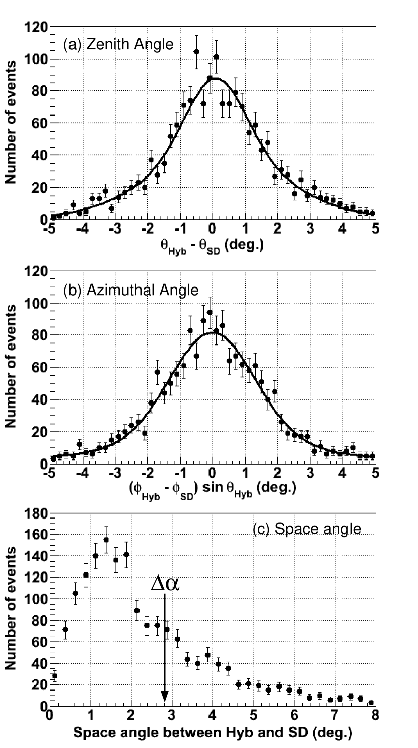
Figure 2: Opening angle distributions of directions measured by hybrid method and SD. Solid curves represent best fits by double-Gaussian function with the common mean value. (a) Opening angle distributions of zenith angles measured by hybrid ($\theta_{\rm Hyb}$) method and SD ($\theta_{\rm SD}$). Estimated mean opening angle is $m=+0\fdg 091\pm 0\fdg 046$. (b) Opening angle of azimuthal angles measured by hybrid ($\phi_{\rm Hyb}$) method and SD ($\phi_{\rm SD}$). Estimated mean opening angle is $m=-0\fdg 022\pm 0\fdg 046$. (c) Space angle distribution of direction measured by the hybrid method and the SD. The vertical arrow indicates a space angle containing 68% of the events ($\Delta\alpha=2\fdg 8\pm 0\fdg 1$).

The performance of the SD was thoroughly verified by a FD-SD hybrid data analysis (Abu-Zayyad et al. 2014a, ) independent of the MC simulation. The arrival directions of the hybrid events were determined by the fluorescence track measured by the FD and the air shower arrival position at the ground measured by the SD. This hybrid reconstruction is almost independent of the SD reconstruction, and its angular resolution, $\sigma_{\rm Hyb}=1\fdg 0\pm 0\fdg 1$, is better than that of the SD reconstruction, $\sigma_{\rm SD}\sim 3\arcdeg$ around 1 EeV. Therefore, the hybrid data are a good reference for estimating the systematic errors in the arrival direction. Figure 2(a) shows the opening angle distributions of the zenith angles measured using the hybrid method ($\theta_{\rm Hyb}$) and the SD ($\theta_{\rm SD}$). Figure 2(b) shows the opening angle distributions of the azimuthal angles measured using the hybrid method ($\phi_{\rm Hyb}$) and the SD ($\phi_{\rm SD}$). The solid curves are fitted to the data points by a double-Gaussian function,

$$G(\delta)=g_{1}(\delta;a_{1},m,\sigma_{1})+g_{2}(\delta;a_{2},m,\sigma_{2}),$$ (2)

where $g_{i}(\delta)=a_{i}e^{-(\delta-m)^{2}/2\sigma_{i}^{2}}$, $i$ indicates the $i$-th Gaussian function, $a_{i}$ is the $i$-th height, $m$ is the common mean value in the two Gaussians, $\sigma_{i}$ is the $i$-th standard deviation, and $\delta$ is the opening angle. The mean opening angles of the zenith angle is calculated to be $m=+0\fdg 091\pm 0\fdg 046$ ($\sigma_{1}=2\fdg 16\pm 0\fdg 12$, $\sigma_{2}=0\fdg 92\pm 0\fdg 10$) using the Chi-squared minimization technique, while that of the azimuthal angle is calculated to be $m=-0\fdg 022\pm 0\fdg 046$ ($\sigma_{1}=3\fdg 63\pm 1\fdg 64$, $\sigma_{2}=1\fdg 30\pm 0\fdg 11$). From these results, the systematic pointing error of the reconstructed SD shower is estimated to be approximately $0\fdg 1$. This is obviously negligible compared with our angular resolution. Figure 2 (c) shows the distribution of the space angle between the directions measured by SD and the hybrid method above 0.5 EeV. A space angle containing 68% of the events $\Delta\alpha$ is estimated to be $2\fdg 8\pm 0\fdg 1$.

We studied the angular resolution of the cosmic-ray arrival directions containing 68% of the reconstructed events, dependence on the zenith angle. In Figure 3, the solid and dashed histograms show the angular resolutions of the MC simulations for proton and iron, respectively. The closed circles show the estimated angular resolution $\sigma_{\rm SD}$ from the following quadratic sum relation.

$$\sigma_{\rm SD}=\sqrt{\Delta\alpha^{2}-\sigma_{\rm Hyb}^{2}},$$ (3)

where, $\Delta\alpha$ is a space angle, containing 68% of the events, between the directions measured by the SD and the hybrid method, which corresponds to Figure 2 (c), $\sigma_{\rm Hyb}=1\fdg 0\pm 0\fdg 1$ is assumed to be the angular resolution of the hybrid method independent of the zenith angle and energy (Abu-Zayyad et al. 2014a, ). The $\sigma_{\rm SD}$ values estimated from the SD-FD hybrid data are in reasonable agreement with the MC simulation results. They agree to better than 3 $\sigma$ for all energy bins. Above 2 EeV, the angular resolution estimated from the hybrid data is slightly better than that from the proton MC, whereas it is consistent with that from the iron MC. Because the composition of primary cosmic rays in this energy region is still under debate owing to the systematic uncertainty, the average difference in angular resolution between the data and the proton MC is defined as a systematic error of the angular resolution, which corresponds to $\sim$15%, assuming the worst case. Thus, these estimations from the hybrid data are good checks for the reconstruction of the TA SD independent of the MC simulation. In Figure 3, the angular resolution is clearly improved at larger zenith angles, and the iron-induced air shower shows slightly better resolution than the proton-induced air shower. This is because the footprint of the air shower at large zenith angles is larger than that at small zenith angles, and the muon component is much greater at large zenith angles than at small zenith angles. The time distribution of muons in an air shower is narrower than that of the electromagnetic components. Therefore, air showers with a high ratio of muons to secondary particles, such as large-zenith-angle or iron-induced air showers, might enable us to better determine the geometry of the air shower front.

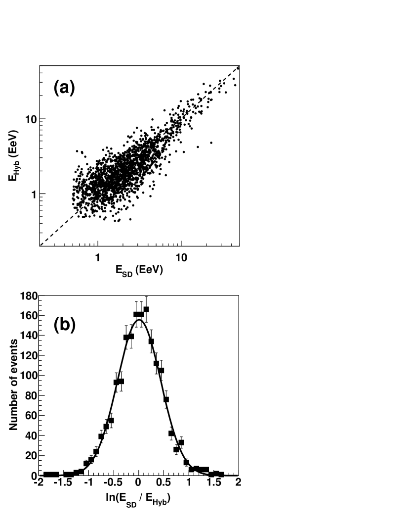
Figure 4: Comparison of reconstructed energies from SD and hybrid method. (a) Scatter plot of reconstructed energy from SD and hybrid method. (b) Natural logarithm of ratio of reconstructed energy from SD and hybrid method. Energy resolution with loose-cut data is estimated to be ${}^{+50}_{-35}$%.

Finally, we estimate the energy resolution of the TA SD with the loose-cut data set using the hybrid data. Figure 4(a) shows a scatter plot of the reconstructed energy from the SD and the hybrid method. Figure 4(b) shows the distribution of the natural logarithm of the ratio of the reconstructed energy from the SD and the hybrid method. The energy resolution of the hybrid analysis is 7%, which is sufficiently better than that of the SD (Abu-Zayyad et al. 2014a, ). From Figure 4, the energy resolution of the SD with the loose-cut data is estimated to be $\sim$${}^{+50}_{-35}$% for $E>1$ EeV, whereas that with the standard-cut data is estimated to be $\sim$${}^{+35}_{-25}$%. This resolution is good enough to find a point-like source if its flux changes gradually with the energy.

5 Background Calculation

Various background estimation methods have been developed to analyze the cosmic-ray anisotropy. A simple method is to compare the distribution of air shower directions generated by the MC simulation directly with the data. In this analysis, the typical number of background events for a target source is up to $\sim$200. To determine the significance of the excess within an accuracy of 0.1 $\sigma$, the background should be estimated as 0.7% ($=\sqrt{200}\times 0.1/200$). However, the MC simulation usually does not reproduce the data with this accuracy due to the simulation model dependence and meteorological effects, which are difficult to incorporate into the MC simulation. In the alternative method, the background can be estimated by the data themselves without the MC simulation. To extract an excess of air shower events coming from the direction of a target source, we adopt the equi-zenith angle method developed by the Tibet AS$\gamma$ experiment (Amenomori et al., 2003) to find gamma-ray excesses from huge cosmic-ray background events in the TeV energy region. The signals are searched for by counting the number of events coming from a target source in an on-source cell with a finite size. The background is estimated by the number of events averaged over six off-source cells with the same angular radius as the on-source cell at the same zenith angle, recorded at the same time as the on-source cell events. Note that the equi-zenith angle method fails when the source object stays at a zenith angle of less than 10$\arcdeg$, because the off-source cells overlap with other cells. Therefore, the air shower events with zenith angles larger than 10$\arcdeg$ were used in this analysis.

The search window size of the on- and off-source cells should be optimized by the MC simulation to maximize the signal-to-noise (S/N) ratio where the signal is the number of detected excess events, and the noise is the square root of the number of background events ($\sqrt{B}$), which depends on the angular resolution. In this MC study, we generated air showers induced by protons, which have the same air shower development as those induced by neutrons. Figure 5 shows S/N ratio as a function of the search window radius $R_{\rm sw}$ in the MC simulation. The vertical axis is the S/N ratio, defined as the number of signals divided by $R_{\rm sw}$ ($=\sqrt{R_{\rm sw}^{2}}$), assuming that the the number of background events ($B$) is proportional to the area of the search window $\pi R_{\rm sw}^{2}$. A peak (arrow position) indicates the optimal search window radius to maximize the S/N ratio. Figure 6 shows the optimal search window radius $R_{\rm sw}$ at the maximum S/N ratio as a function of the zenith angle $\theta$ and the results of fitting by an empirical formula, $R_{\rm sw}(\theta)=R_{0}{\rm cos}\theta$, where $R_{0}$ is the fitting parameter denoting the window radius for a vertical air shower. The calculated $R_{0}$ values are $3\fdg 1$, $2\fdg 9$, and $2\fdg 1$ for three energy regions: $0.5<E{\rm(EeV)}\leq 1.0$, $1.0<E{\rm(EeV)}\leq 2.0$, and $E{\rm(EeV)}>2.0$, respectively. In this analysis, we use these fitting curves in Figure 6 as the optimal search window radius. If the signals show a normal Gaussian distribution, the optimal window size $R_{\rm sw}(\theta)$ should be close to the angular resolution $\sigma_{\rm SD}$. $R_{\rm sw}(\theta)$ is, however, $0.6\sim 0.7$ times smaller than $\sigma_{\rm SD}$ because the signal spread shows a large-tail distribution.

The off-source cells are located in the azimuthal direction at the same zenith angle as the on-source direction. Four off-source cells are symmetrically aligned on each side of the on-source cell, at $6\fdg 4$ steps from the on-source position measured in terms of the real angle, and pick up events recorded at the same time to the on-source cell. This method, the so-called equi-zenith angle method, can reliably estimate the background events under the same conditions as those for the on-source events. Here, it is worth noting that the two off-source cells adjacent to the on-source cell are excluded to avoid possible signal tail leakage into the off-source events. Therefore, the total number of off-source cells is six. The TA SD has the anisotropy of 6% at the maximum in the azimuthal direction owing to the azimuthal dependence of the trigger efficiency. This anisotropy, which is well understood, appears along the grid of detector arrangement for the air showers with small number of hit detectors. To correct this anisotropy, we analyzed 19 dummy sources, which follow the same diurnal rotation (at the same declination and a spacing of 18$\arcdeg$ in right ascension, except for the location of the object itself) in the same way as for the target source using the equi-zenith angle method. The background distribution of the mean values of the observed air shower events for the 19 dummy sources reproduces the background shape of the object at the same declination very well (Amenomori et al., 2003). The number of events in the $i$-th off-source cell of the target source $n_{\rm off}^{i}$ is corrected by the number of events at the on- and off-source cells averaged over the 19 dummy sources using the following equation:

$$N_{\rm off}^{i}=n_{\rm off}^{i}\left(\frac{\langle D_{\rm on}\rangle}{\langle D_{\rm off}^{i}\rangle}\right),$$ (4)

where $N_{\rm off}^{i}$ is the corrected number of events at the $i$-th off-source cell, $\langle D_{\rm off}^{i}\rangle$ is the number of events averaged over the 19 dummy sources at the $i$-th off-source cell, and $\langle D_{\rm on}\rangle$ is the number of events averaged over the 19 dummy sources at the on-source cell. This correction enables us to remove the anisotropy of off-source events completely if the azimuthal anisotropy is stable. This is because the 19 dummy sources are observed on a different part of the sky every day, as they all orbit with the same diurnal rotation. The correction factors $\langle D_{\rm on}\rangle/\langle D_{\rm off}^{i}\rangle$ are $1.0\pm 0.03$ which depends on the declination.

Finally, we calculate the statistical significance of cosmic-ray signals from the target sources against cosmic-ray background events using the following formula (Li & Ma, 1983):

$$S_{\rm LM}=\sqrt{2}\left[N_{\rm on}~{}{\rm ln}\left(\frac{(1+\eta)N_{\rm on}}{\eta(N_{\rm on}+N_{\rm off})}\right)+N_{\rm off}~{}{\rm ln}\left(\frac{(1+\eta)N_{\rm off}}{N_{\rm on}+N_{\rm off}}\right)\right]^{1/2},$$ (5)

where $N_{\rm on}$, $N_{\rm off}$, and $\eta$ are the number of events in the on-source cell, the number of corrected background events summed over six off-source cells ($N_{\rm off}=\sum_{i=1}^{6}N_{\rm off}^{i}$), and the ratio of the on-source solid angle area to the off-source solid angle area ($\eta$ = 1/6 in this work), respectively.

6 Results and Discussion

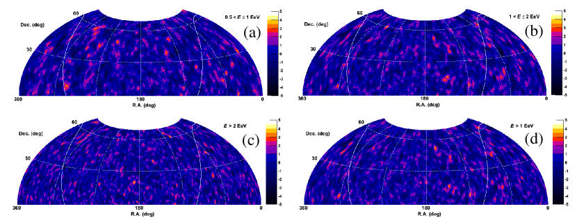
Figure 7: Significance maps of the northern sky between Dec. = 0$\arcdeg$ and Dec. = $70\arcdeg$ surveyed by TA SD in four energy regions: (a) $0.5<E{\rm(EeV)}\leq 1.0$, (b) $1.0<E{\rm(EeV)}\leq 2.0$, (c) $E{\rm(EeV)}>2.0$, (d) $E{\rm(EeV)}>1.0$. Color contours show significance level. Solid curves indicate the Galactic plane.

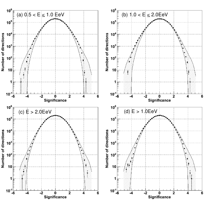
Figure 8: Histograms showing significance distributions in all directions within FoV of TA SD in four energy regions: (a) $0.5<E{\rm(EeV)}\leq 1.0$, (b) $1.0<E{\rm(EeV)}\leq 2.0$, (c) $E{\rm(EeV)}>2.0$, (d) $E{\rm(EeV)}>1.0$. Shaded area indicates 95% containment region of 10⁵ MC samples of isotropic sky.

We analyze 180,644 air showers collected by the TA SD from 2008 May 11 to 2013 May 4. Figure 7 shows the northern significance sky map drawn by the equi-zenith angle method using cosmic rays observed by the TA SD in the four energy regions. In this analysis, to ensure that we did not miss any possible unknown sources, the surveyed sky was oversampled. The centers of the tested target sources are set on $0\fdg 1\times 0\fdg 1$ grids, from 0$\arcdeg$ to 360$\arcdeg$ in right ascension and from 0$\arcdeg$ to 70$\arcdeg$ in declination. At each grid point, a search window with the optimal radius $R_{\rm sw}(\theta)$, as shown in Figure 6, was opened. The observed declination band is limited by the statistics and the analysis method. The number of events at Dec.$<0\arcdeg$ is small. At Dec. $>70\arcdeg$, near the northern pole, the dummy source cells overlap other cells, so the statistical independence of each cell fails. The closed circles in Figure 8 show the significance distributions from all directions in the four energy regions. The shaded area is the 95% containment region of 10⁵ MC samples in the isotropic sky. The good agreement between the data points and shaded area indicates that there is overall no significant excess beyond the statistical fluctuation in the northern sky.

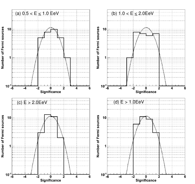
Figure 9: Histograms showing significance distributions of 29 Fermi bright Galactic sources within FoV of TA SD in four energy regions: (a) $0.5<E{\rm(EeV)}\leq 1.0$, (b) $1.0<E{\rm(EeV)}\leq 2.0$, (c) $E{\rm(EeV)}>2.0$, (d) $E{\rm(EeV)}>1.0$. Dotted curves are expected normal Gaussian distributions.

Subsequently, we also searched for coincidence with the Fermi bright Galactic sources. The target sources in the Fermi bright source list (Abdo et al. 2009a, ) were chosen as confirmed or potential Galactic sources in the same way as for the TeV observations of the Milagro and Tibet AS$\gamma$ (Abdo et al. 2009b, ; Amenomori et al., 2010). Out of the 205 most significant sources in the Fermi bright source list, 84 are not identified as extragalactic sources. Among these 84, we selected 29 sources in the declination band between 0$\arcdeg$ and 70$\arcdeg$, corresponding to the sensitive FoV of the TA SD. The results of the search for neutral particles from the 29 Fermi bright Galactic sources are summarized in Table 2, where 15 of the selected sources are classified as pulsars (PSR), 5 are supernova remnants (SNR), 1 is a high-mass X-ray binary (HXB), and 8 remain unidentified but are potential Galactic sources; they are mostly concentrated in the Galactic plane ($|b|<\sim 20\arcdeg$) (Abdo et al. 2009a, ). Many Fermi bright Galactic sources are confirmed sources at TeV energies, as shown in Table 2. Figure 9 shows the significance distributions of the 29 Fermi source directions searched by the TA SD. The distributions are obviously consistent with the normal Gaussian distribution, indicating that there are no statistically significant signals from these sources.

We calculated the flux upper limits on the neutron intensity ($F_{\rm ul}$) of the northern sky using the following equation:

$$F_{\rm ul}=F_{\rm cr}\frac{N_{\rm ul}}{N_{\rm bg}}\frac{\omega_{\rm sw}}{\epsilon_{\rm sw}},$$ (6)

where $F_{\rm cr}$ is the integral cosmic-ray flux; $N_{\rm ul}$ is the upper limit on the observed excess $(N_{\rm on}-N_{\rm bg})$ according to a statistical prescription assuming an unphysical region, such as a region of negative excess (Helene, 1983); $N_{\rm bg}(=\eta N_{\rm off}$) is the average number of background events; $\omega_{\rm sw}$ is the averaged solid angle of the search window for a target source depending on the declination; and $\epsilon_{\rm sw}$ is the signal efficiency with the angular cut by $\omega_{\rm sw}$ deduced from the MC simulation of proton ($\sim$ neutron) assuming a point source. The $F_{\rm cr}$ values at $0.5$ EeV, $1$ EeV, and $2$ EeV are assumed to be fluxes measured by HiRes (Abbasi et al., 2008) because the TA spectrum below 10^18.2 eV has not been published yet. The HiRes spectrum is consistent with that of the TA within 5% at 10^18.2 eV. The value of $\epsilon_{\rm sw}$ is estimated to be $0.50\pm 0.01$ for energies between 0.5 EeV and 1.0 EeV, and $0.45\pm 0.01$ for $E>1$ EeV, independent of the declination of the target source. The typical fractions of the upper excess ($N_{\rm ul}/N_{\rm bg}$) in each energy bin are 29% for $0.5<E{\rm(EeV)}\leq 1.0$, 29% for $1.0<E{\rm(EeV)}\leq 2.0$, 46% for $E{\rm(EeV)}>2.0$, and 25% for $E{\rm(EeV)}>1.0$. First, we calculated the flux upper limit of the entire northern sky point by point on $0\fdg 1\times 0\fdg 1$ grids using Eq. 6. Then, the mean of the flux limits at the same declination was defined as the representative value at each declination. Figure 10 shows the representative mean flux upper limits (km^-2 yr^-1) at the 95% C.L. in the four energy regions according to the declination of the target sources. The average flux upper limit in the northern sky is estimated to be 0.07 km^-2 yr^-1 for $E>1$ EeV. This is the most stringent flux upper limit in a northern sky survey assuming point-like sources. The flux upper limit for each Fermi bright Galactic source is also listed in Table 2.

The fluxes of Cygnus X-3 reported by the Fly’s Eye and the Akeno 20-km² array are $(2.0\pm 0.6)\times 10^{-17}$ cm^-2 s^-1 and $(1.8\pm 0.7)\times 10^{-17}$ cm^-2 s^-1 for $E>0.5$ EeV, respectively (Cassiday et al., 1989; Teshima et al., 1990). Our observational results for Cygnus X-3 are summarized in Table 3. The upper limit at the 95% C.L. on the neutron flux of Cygnus X-3 observed by the TA SD is estimated to be 0.2 km^-2 yr^-1 (=$5.6\times 10^{-19}$ cm^-2 s^-1) for $E>0.5$ EeV, as shown in Table 3. This is an order of magnitude smaller than the fluxes measured by the Fly’s Eye and the Akeno 20-km² array. One possible explanation of their signals around Cygnus X-3 could be transient emission during their observation periods. We divided the data set between 2008 May 11 and 2013 May 4 into 18 periods (1 period $\sim$100 days) and searched for transient signals from Cygnus X-3. We found no significant excess in these 18 periods.

7 Summary

We search for steady point-like sources of neutral particles in the EeV energy range observed by the TA SD, which has the largest effective area in the northern sky. The data selection was loosen and tuned the reconstruction of the arrival direction in this analysis. As a result, the number of air showers with $E>0.5$ EeV, which corresponds to 180,644 events, was $\sim$10 times larger than the original “standard cut” analysis around EeV energies. To search for point-like sources, the equi-zenith angle method was applied to these cosmic-ray air showers taken by the TA SD between 2008 May and 2013 May. We found no significant excess for $E>0.5$ EeV in the northern sky. Subsequently, we also searched for coincidence with the Fermi bright Galactic sources. No significant coincidence was found within the statistical error. Hence, we set upper limits at the 95% C.L. on the neutron flux, which is an averaged flux of 0.07 km^-2 yr^-1 for $E>1$ EeV in the northern sky. This is the most stringent flux upper limit in a northern sky survey assuming point-like sources. The upper limit at the 95% C.L. on the neutron flux of Cygnus X-3 is estimated to be 0.2 km^-2 yr^-1 for $E>0.5$ EeV. This is an order of magnitude lower than the previous flux measurements.

Figure 1: Reconstructed energy distributions. Closed circles and triangles show energy distributions of experimental data after loose and standard cuts, respectively. Solid and dashed histograms show energy distributions in MC simulation after loose and standard cuts, respectively. The areas of MC simulation are normalized to those of the data.

Figure 3: Angular resolutions of TA SD as a function of zenith angle. Solid histograms show results of MC simulation assuming pure protons. Dashed histograms show results of MC simulation assuming pure iron. Closed circles indicate the estimated angular resolution from opening angles of reconstructed directions between SD and hybrid data. Zenith angle of hybrid data is limited to $55\arcdeg$. MC simulation and hybrid data are divided into three energy regions: (a) $0.5<E{\rm(EeV)}\leq 1.0$ (upper panel), (b) $1.0<E{\rm(EeV)}\leq 2.0$ (middle panel), (c) $E{\rm(EeV)}>2.0$ (lower panel).

Figure 5: S/N curves for vertical air showers ($\theta<5\arcdeg$) as a function of search window size $R_{\rm sw}$ from MC simulation in three energy regions: (a) $0.5<E{\rm(EeV)}\leq 1.0$, (b) $1.0<E{\rm(EeV)}\leq 2.0$, (c) $E{\rm(EeV)}>2.0$. The solid curves are a spline fitting to the MC data as shown by the points. Noise ($=\sqrt{B}$, square root of number of background events) is proportional to the area of the search window $\pi R_{\rm sw}^{2}$. Peak (solid arrow) indicates optimal search window radius to maximize S/N ratio.

Figure 6: Optimal search window radius as a function of zenith angle $\theta$ from MC simulation. The curves show the best fit by the empirical formula $R_{\rm sw}=R_{0}~{}{\rm cos}\theta$. Symbols and line types represent theree different energy regions: squares with solid curve, $0.5<E{\rm(EeV)}\leq 1.0$; circles with dotted curve, $1.0<E{\rm(EeV)}\leq 2.0$; triangles with dashed curve, $E{\rm(EeV)}>2.0$.

Figure 10: Mean flux upper limits (km^-2 yr^-1) at 95% C.L. according to the declination of the target sources observed by TA SD at each energy. Dot-dashed curve: $0.5<E{\rm(EeV)}\leq 1.0$; dashed curve: $1.0<E{\rm(EeV)}\leq 2.0$; dotted curve: $E{\rm(EeV)}>2.0$; solid curve: $E{\rm(EeV)}>1.0$.

Table 1: Loose-cut parameters in this analysis and the number of remaining events

Cut parameters	# of events
# of triggered events	1,133,213
# of SDs $\geq 4$	296,208
Pointing direction error $<10\arcdeg$	290,603
Zenith angle $\theta<55\arcdeg$	255,332
Energy $>$ 0.5 EeV	180,644

Table 2: Results of search for EeV neutral particles from the 29 Fermi Galactic sources

Fermi LAT		R.A.	Dec.	$S_{\rm LM}$ ($>$1EeV)	$F_{\rm ul}$($>$1EeV)		Source
Source(0FGL)	Class	(deg.)	(deg.)	($\sigma$)	(km-2 yr-1)	TeV $\gamma$	Associations
J0030.3+0450	PSR	7.6	4.8	$-$0.15	$<$0.07
J0240.3+6113	HXB	40.0	61.2	$-$0.35	$<$0.05	Yes
J0357.5+3205	PSR	59.3	32.0	$-$1.19	$<$0.04
J0534.6+2201	PSR	83.6	22.0	$-$0.36	$<$0.06	Yes	Crab
J0617.4+2234	SNR	94.3	22.5	+1.20	$<$0.11	Yes	IC 443
J0631.8+1034	PSR	97.9	10.5	$-$0.29	$<$0.07
J0633.5+0634	PSR	98.3	6.5	$-$0.29	$<$0.06
J0634.0+1745	PSR	98.5	17.7	+0.21	$<$0.09		Geminga
J0643.2+0858	-	100.8	8.9	$-$0.99	$<$0.05
J1830.3+0617	-	277.5	6.2	+0.93	$<$0.12
J1836.2+5924	PSR	279.0	59.4	$-$0.76	$<$0.04
J1855.9+0126	SNR	283.9	1.4	+0.90	$<$0.11		W44
J1900.0+0356	-	285.0	3.9	+0.73	$<$0.11
J1907.5+0602	PSR	286.8	6.0	+0.84	$<$0.10	Yes
J1911.0+0905	SNR	287.7	9.0	$-$0.85	$<$0.05	Yes	G43.3$-$0.17
J1923.0+1411	SNR	290.7	14.1	$-$1.31	$<$0.04	Yes	W51
J1953.2+3249	PSR	298.3	32.8	$-$1.54	$<$0.04
J1954.4+2838	SNR	298.6	28.6	+0.47	$<$0.09		G65.1+0.6
J1958.1+2848	PSR	299.5	28.8	+0.70	$<$0.09
J2001.0+4352	-	300.2	43.8	$-$0.76	$<$0.05
J2020.8+3649	PSR	305.2	36.8	$-$0.93	$<$0.05	Yes
J2021.5+4026	PSR	305.3	40.4	$-$0.24	$<$0.07
J2027.5+3334	-	306.8	33.5	+0.77	$<$0.11
J2032.2+4122	PSR	308.0	41.3	$-$1.25	$<$0.04	Yes
J2055.5+2540	-	313.8	25.6	+1.04	$<$0.10
J2110.8+4608	-	317.7	46.1	$-$1.63	$<$0.03
J2214.8+3002	PSR	333.7	30.0	+0.55	$<$0.09
J2229.0+6114	PSR	337.2	61.2	+1.13	$<$0.09	Yes
J2302.9+4443	-	345.7	44.7	$-$1.50	$<$0.03

Table 3: Summary of Cygnus X-3 observations by the TA SD

Energy(EeV)	$E>0.5$			$E>1.0$			$E>2.0$
	$S_{\rm LM}$	$F_{\rm ul}$		$S_{\rm LM}$	$F_{\rm ul}$		$S_{\rm LM}$	$F_{\rm ul}$
Object	($\sigma$)	(km-2 yr-1)		($\sigma$)	(km-2 yr-1)		($\sigma$)	(km-2 yr-1)
Cygnus X-3	$-$1.04	$<$0.2		$-$1.55	$<$0.03		$-$0.24	$<$0.02

References

- Abbasi et al. (2007) Abbasi, R. U., Abu-Zayyad, T., Amann, J. F., et al. 2007, Astropart. Phys., 27, 512
- Abbasi et al. (2008) Abbasi, R. U., Abu-Zayyad, T., Allen, M., et al. 2008, Phys. Rev. Lett., 100, 101101
- Abbasi et al. (2014) Abbasi, R. U., Abe, M., Abu-Zayyad, T., et al. 2014, ApJ, 790, L21
- (4) Abdo, A. A., Ackermann, M., Ajello, M., et al. 2009a, ApJS, 183, 46
- (5) Abdo, A. A., Allen, B. T., Aune, T., et al. 2009b, ApJ, 700, L127
- Abreu et al. (2012) Abreu, P., Aglietta, M., Ahlers, M., et al. 2012, ApJ, 760, 148
- (7) Abu-Zayyad, T., Aida, R., Allen, M., et al. 2012a, ApJ, 757, 26
- (8) Abu-Zayyad, T., Aida, R., Allen, M., et al, 2012b, NIM-A, 689, 87
- (9) Abu-Zayyad, T., Aida, R., Allen, M., et al. 2013a, ApJ, 768, L1
- (10) Abu-Zayyad, T., Aida, R., Allen, M., et al. 2013b, Astropart. Phys., 48, 16
- (11) Abu-Zayyad, T., Aida, R., Allen, M., et al. 2014a, Astropart. Phys., in press (arXiv:1305.7273)
- (12) Abu-Zayyad, T., Aida, R., Allen, M., et al. 2014b, Astropart. Phys., in press (arXiv:1403.0644)
- (13) Abu-Zayyad, T., Aida, R., Allen, M., et al. 2013d, ApJ, 777, 88
- (14) Abu-Zayyad, T., Aida, R., Allen, M., et al. 2013e, Phys. Rev. D, 88, 112005
- Amenomori et al. (2003) Amenomori, M., Ayabe, S., Cui, S. W., et al. 2003, ApJ, 598, 242
- Amenomori et al. (2010) Amenomori, M., Bi, X. J., Chen, D., et al. 2010, ApJ, 809, L6
- Cassiday et al. (1989) Cassiday, G. L., Cooper, R., Dawson, B. R., et al. 1989, Phys. Rev. Lett., 62, 383
- d’Orfeuil et al. (2011) d’Orfeuil, B. R., & The Pierre Auger Collaboration 2011, Proceedings of 32nd ICRC (Beijing), 2, 91 (arXiv:1107.4805)
- Fukushima et al. (2013) Fukushima, M., Ivanov, D., Kawata, K., et al. 2013, Proceedings of 33rd ICRC (Rio de Janeiro), CR-EX (Id:1033), in press
- Greisen (1966) Greisen, K. 1966, Phys. Rev. Lett., 16, 748
- Heck et al. (1998) Heck, D., Knapp, J., Capdevielle, J. N., Shatz, G., & Thouw, T. 1998, CORSIKA: A Monte Carlo Code to Simulate Extensive Air Showers (FZKA 6019)(Karlsruhe: Forschungszentrum Karlsruhe)
- Helene (1983) Helene, O. 1983, Nucl. Instrum. Methods Phys. Res., 212, 319
- Lawrence et al. (1989) Lawrence, M. A., Prosser, D. C. & Watson, A. A. 1989, Phys. Rev. Lett., 63, 1121
- Li & Ma (1983) Li, T.-P., & Ma, Y.-Q. 1983, ApJ, 272, 317
- Linsley & Scarsi (1962) Linsley, J., & Scarsi, L. 1962, Phys. Rev., 128, 2384
- Nelson et al. (1985) Nelson, W. R., Hirayama, H., & Rogers, D. W. O. 1985, Report No. SLAC-0265
- Stokes et al. (2012) Stokes, B. T., Cady, R., Ivanov, D., Matthews, J. N. & Thomson, G. B. 2012, Astropart. Phys., 35, 759
- Tameda (2013) Tameda, Y. & The Telescope Array Collaboration 2013, Proceedings of 33rd ICRC (Rio de Janeiro), CR-EX (Id:512), in press
- Teshima et al. (1986) Teshima, M., Matsubma, Y., Hara, T., et al. 1986, J. Phys. G: Nucl. Phys., 12, 1097
- Teshima et al. (1990) Teshima, M., Matsubara, Y., Nagano, M., et al. 1990, Phys. Rev. Lett., 64, 1628
- Tokuno et al. (2012) Tokuno, H., Tameda, Y., Takeda, M., et al. 2012, NIM-A, 676, 54
- Udo et al. (2007) Udo, S., Allen, M., Cady, R., et al. 2007, 30th ICRC (Merida), Proceedings of 30th ICRC (Merida), Ed. R. Caballero, et al. (Universidad Nacional Autonoma de Mexico, Mexico City, Mexico), 5, 1021
- Zatsepin & Kuz’min (1966) Zatsepin, G. T., & Kuz’min, V. A. 1966, J. Exp. Theor. Phys. Lett., 4, 78