A six-part collisional model of the main asteroid belt

Abstract

In this work, we construct a new model for the collisional evolution of the main asteroid belt. Our goals are to test the scaling law of Benz and Asphaug (1999) and ascertain if it can be used for the whole belt. We want to find initial size-frequency distributions (SFDs) for the considered six parts of the belt (inner, middle, “pristine”, outer, Cybele zone, high-inclination region) and to verify if the number of synthetic asteroid families created during the simulation matches the number of observed families as well. We used new observational data from the WISE satellite (Masiero et al., 2011) to construct the observed SFDs. We simulate mutual collisions of asteroids with a modified version of the Boulder code (Morbidelli et al., 2009), where the results of hydrodynamic (SPH) simulations of Durda et al. (2007) and Benavidez et al. (2012) are included. Because material characteristics can significantly affect breakups, we created two models — for monolithic asteroids and for rubble-piles. To explain the observed SFDs in the size range $D=1$ to 10 km we have to also account for dynamical depletion due to the Yarkovsky effect. The assumption of (purely) rubble-pile asteroids leads to a significantly worse fit to the observed data, so that we can conclude that majority of main-belt asteroids are rather monolithic. Our work may also serve as a motivation for further SPH simulations of disruptions of smaller targets (with a parent body size of the order of 1 km).

1 Introduction

The collisional evolution of the main asteroid belt has been studied for more than 60 years (Dohnanyi (1969), Davis et al. (1979) etc.). The first collisional model was created by Dohnanyi (1969) and his important result was that a size-frequency distribution for a population of mutually colliding asteroids will reach an equlibrium. If the cumulative distribution is described by a power law, the corresponding slope (exponent) will be close to $-2.5$. An overview of previous modelling of the main belt and subsequent advances can be found in a relatively recent paper by Bottke et al. (2005), so that we shall not repeat it here. Nevertheless, it is worth to mention another development, which is an attempt to merge a classical particle-in-a-box collisional model with (parametrized) results of smooth-particle hydrodynamic (SPH) codes as done in Morbidelli et al. (2009). We are going to use this kind of method in this work.

Every collisional model should comply with two important constraints: 1) the size-frequency distribution (SFD) of main belt at the end of a simulation must fit the observed SFD; 2) the number of asteroid families created during this simulation must fit the observed number of families. It is important to note, that the models were improved in the course of time not only due to the progress of technology or new methods but also thanks to an increasing amount of observational data. In this work, we could exploit new data obtained by the WISE satellite (Wide-field Infrared Survey Explorer; Masiero et al., 2011), specifically, diameters and geometric albedos for 129,750 asteroids.

Moreover, several tens of asteroid families are observed in the main belt as shown by many authors (Zappalà et al., 1995; Nesvorný et al., 2005; Nesvorný, 2010; Brož et al., 2013; Masiero et al., 2013; Milani et al., 2013). The lists of collisional families are also steadily improved, they become more complete and (luckily) compatible with each other.

In order to fully exploit all new data, we created a new collisional model in which we divided the whole main belt into six parts (see Section 2 for a detailed discussion and Section 3 for the description of observational data). Our aims are: 1) to check the number of families in individual parts of the belt — we use the list of families from Brož et al. (2013) (which includes also their physical properties) with a few modifications; 2) to verify whether a single scaling law (e.g. Benz and Asphaug, 1999) can be used to fit the whole asteroid belt, or it is necessary to use two different scaling laws, e.g. one for the inner belt and second for the outer belt; 3) and we also test a hypothesis, if the main belt is mostly composed of monolithic or rubble-pile objects.

In this paper, we assume that all families observed today were created in the last $\sim 4\,{\rm Gyr}$ (without any influence of the late heavy bombardment dated approximately $4.2$ to $3.85\,{\rm Gyr}$ ago). We thus focus on an almost steady-state evolution of the main belt, without any significant changes of collisional probabilities or dynamical characteristics. This is different from the work of Bottke et al. (2005). We must admit here that the assumption of the steady-state evolution could be disputable, since Dell’Oro et al. (2001) showed that the formation of big asteroid families may influence the impact probability.

We model collisions with the statistical code called Boulder (Morbidelli et al., 2009) that we slightly extended to account for six populations of asteroids (Sections 5, 6). As mentioned above, the Boulder code incorporates the results of the SPH simulations by Durda et al. (2007) for monolithic $D_{\rm PB}=100\,{\rm km}$ parent bodies, namely for the masses of the largest remnant and fragment and an overall slope of fragment’s SFD. For asteroids larger or smaller than $D_{\rm PB}=100\,{\rm km}$ a scaling is used for sake of simplicity.

Material characteristics definitely have significant influence on mutual collisions (e.g. Michel et al., 2011; Benavidez et al., 2012). Therefore, we also run simulations with rubble-pile objects, which are less firm (refer to Section 7). A set of simulations analogous to Durda et al. (2007) for rubble-pile targets with $D_{\rm PB}=100\,{\rm km}$ was computed by Benavidez et al. (2012).

First, we try to explore the parameter space using a simplex algorithm while we keep the scaling law fixed. Considering a large number of free parameters and the stochasticity of the system, we look only for some local minima of $\chi^{2}$ and we do not expect to find a statistically significant global minimum. Further possible improvements and extensions of our model are discussed in Sections 8 and 9.

2 A definition of the six parts of the main belt

Figure 1: A definition of the six parts of the main asteroids belt according to the semimajor axis $a$ and the inclination $I$: inner, middle, “pristine”, outer, Cybele zone and high-inclination region. The numbers of objects in these parts are the following: 177,756; 186,307; 23,132; 121,186; 1,894 and 25,501, respectively.

We divided the main belt into six parts (sub-populations) according the synthetic orbital elements (the semimajor axis $a$ and the inclination $I$, Figure 1). Five parts separated by major mean-motion resonances with Jupiter are well-defined — if an asteroid enters a resonance due to the Yarkovsky effect (Bottke et al., 2006), its eccentricity increases and the asteroid becomes a near-Earth object. Consequently, vast majority of large asteroids do not cross the resonances and we do not account for resonance crossing in our model. The sixth part is formed by asteroids with high inclinations, $\sin I_{\rm p}>0.34$. This value corresponds approximately to the position of the $\nu_{6}$ secular resonance.

Namely, the individual parts are defined as follows:

1. inner belt – from $a=2.1$ to 2.5 AU (i.e. the resonance 3:1);

2. middle belt – from 2.5 to 2.823 AU (5:2);

3. “pristine” belt – from 2.823 to 2.956 AU (7:3; as explained in Brož et al. 2013);

4. outer belt – from 2.956 to 3.28 AU (2:1);

5. Cybele zone – from 3.3 to 3.51 AU;

6. high-inclination region – $\sin I>0{.}34$.

For $a$ and $\sin I$ we preferentially used the proper values from the AstDyS catalogue (Asteroids Dynamic Site; Knežević and Milani, 2003). For remaining asteroids, not included in AstDyS, we used osculating orbital elements from the AstOrb catalogue (The Asteroid Orbital Elements Database).

More precisely, we used proper values from AstDyS for 403,674 asteroids and osculating values from AstOrb for 132,102 not-yet-numbered (rather small) asteroids, which is a minority. We thus think that mixing of proper and osculating orbital elements cannot affect the respective size-frequency distributions in a significant way. Moreover, if we assign (erroneously) e.g. a high-inclination asteroid to the outer main belt, then it is statistically likely that another asteroid from the outer main belt may be assigned (erroneously) to the high-inclination region, so that overall the SFDs remain almost the same.

3 Observed size-frequency distributions

To construct SFDs we used the observational data from the WISE satellite (Masiero et al., 2011) — for 123,306 asteroids. Typical diameter and albedo relative uncertainties are $\sim 10\%$ and $\sim 20\%$, respectively (Mainzer et al., 2011), but since we used a statistical approach ($10^{4}$ to $10^{5}$ bodies), this should not present a problem. For asteroids not included there we could exploit the AstOrb catalogue (i.e. data from IRAS; Tedesco et al., 2002) — for 451 bodies. For remaining asteroids (412,019), we calculated their diameters according the relation (Bowell et al., 1989)

$$D=10^{0.5\left(6.259-{\rm log}\,p_{V}\right)-0.4\,H}\,,$$ (1)

where $H$ denotes the absolute magnitude from the AstOrb catalogue and $p_{V}$ the (assumed) geometric albedo. We assigned albedos to asteroids without a known diameter randomly, by a Monte-Carlo method, from the distributions of albedos constructed according to the WISE data. Differences in albedo distributions can influence the resulting SFDs, therefore for each part of the main belt, we constructed a distribution of albedos separately.

We checked that the WISE distributions of albedos are (within a few percent) in agreement with the distributions found by Tedesco et al. (2005). The (minor) differences can be attributed for example to a substantially larger sample (119,876 asteroids compared to 5,983), which includes also a lot of asteroids with smaller sizes ($D\lesssim 10\,{\rm km}$). The resulting observed SFDs are shown in Figure 2. We can see clearly that the individual SFDs differ significantly in terms of slopes and total numbers of asteroids.

Figure 2: The observed cumulative size-frequency distributions $N({>}D)$ of the six parts of the main belt. We used the observational data from the WISE satellite (Masiero et al., 2011) and the AstOrb catalogue for their construction. For asteroids which have no albedos in the WISE database, we assigned albedos by a Monte Carlo method from the distribution of WISE albedos.

To verify a validity of this method, we perform the following test (for the whole main belt). We assume a known set of diameters. We then assign albedos randomly to the individual diameters according to the distribution of WISE albedos. We calculate the values of the absolute magnitudes $H$ by the inversion of Eq. (1). Now, we try to reconstruct the SFD from $H$ and $p_{V}$. The new ”unknown“ values of diameters are computed according to Eq. (1) and for the values of $p_{V}$ we test three following options: 1) a fixed albedo $p_{V}=0.15$; 2) the mean value $p_{V}=0.13$ (derived from the distribution of WISE albedos); 3) for $H<15\,{\rm mag}$ we used the known albedos, for other bodies we assigned albedos by the Monte-Carlo method as above. The known SFD and the three reconstructed SFDs are shown in Figures 3.

The largest uncertainties of the reconstruction are given by the method of assignment of geometric albedos, but we verified that the third method is the best one and that these uncertainties (Figure 3) are much smaller than the differences between individual SFDs (Figure 2).

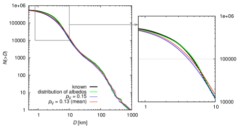
Figure 3: A test of three reconstructions of a ”known“ size-frequency distribution. Diameters were calculated according to Eq. (1) and for values of $p_{V}$ we try to use: 1) $p_{V}=0.15$ (blue line), 2) $p_{V}=0.13$, i.e. the mean value from the distribution of WISE albedos (red line), and 3) we used albedos from WISE for $H<15\,{\rm mag}$; for other bodies we assigned albedos by a Monte-Carlo method according to the distribution of WISE albedos (green line). We can see that the third method is the best one.

Another possible difficulty, especially for asteroids with diameters $D<10\,{\rm km}$, is the observational bias. In Figure 2, we can see that for sizes smaller than some $D_{\rm limit}$ the total number of asteroids remains constant. We also probably miss same asteroids with $D_{\rm limit}<D<10\,$km. These objects are less bright than the reach of current surveys: LINEAR (Stuart, 2001), Catalina, Spacewatch (Bottke et al., 2002), or Pan-STARRS (Hodapp et al., 2004). Nevertheless, for $D>10\,{\rm km}$ we do not need to perform debiasing and neither for smaller asteroids we do not account for the bias, because the range of diameters $D$ where we fit out model is limited (see Table 4).

4 Collisional probabilities and impact velocities

To model the collisional evolution of the main belt by the Boulder code we need to know the intrinsic probabilities $p_{\rm i}$ of collisions between individual parts and the mutual impact velocities $v_{\rm imp}$. The values of $p_{\rm i}$ and $v_{\rm imp}$ were computed by the code written by W.F. Bottke (Bottke and Greenberg, 1993; Greenberg, 1982). For this calculation, we used only the osculating elements from the AstOrb catalogue.

We calculated $p_{\rm i}$’s and $v_{\rm imp}$’s between each pair of asteroids of different populations. We used first 1,000 asteroids from each population (first according to the catalogue nomenclature). We checked that this selection does not significantly influence the result. We constructed the distributions of eccentricities and inclinations of first 1,000 objects from each region and we verified that they approximately correspond with the distributions for the whole population. We also tried a different selection criterion (last 1,000 orbits), but this changes neither $p_{\rm i}$ nor $v_{\rm imp}$ values substantially.

From these sets of $p_{\rm i}$’s and $v_{\rm imp}$’s, we computed the mean values $\overline{p_{\rm i}}$ and $\overline{v}_{\rm imp}$ (for $v_{\rm imp}$ only if corresponding $p_{\rm i}\neq 0$). We checked that the distributions are relatively close to the Gauss distribution and the computations of the mean values are reasonable.

Table 1: The computed intrinsic collisional probabilities $\overline{p_{\rm i}}$ and the mutual impact velocities $\overline{v}_{\rm imp}$ (for $v_{\rm imp}$ only if $p_{\rm i}\neq 0$) between objects belonging to the different parts of the main belt. The uncertainties are of the order $0.1\times 10^{-18}\,{\rm km}^{-2}\,{\rm yr}^{-1}$ for $\overline{p_{\rm i}}$ and $0.1\,{\rm km}\,{\rm s}^{-1}$ for $\overline{v}_{\rm imp}$.

interacting	$\overline{p_{\rm i}}$	$\overline{v}_{\rm imp}$
populations	$(10^{-18}\,{\rm km}^{-2}\,{\rm yr}^{-1})$	$({\rm km\,s}^{-1})$
inner – inner	11.98	4.34
inner – middle	5.35	4.97
inner – pristine	2.70	3.81
inner – outer	1.38	4.66
inner – Cybele	0.35	6.77
inner – high inc.	2.93	9.55
middle – middle	4.91	5.18
middle – pristine	4.67	3.96
middle – outer	2.88	4.73
middle – Cybele	1.04	5.33
middle – high inc.	2.68	8.84
pristine – pristine	8.97	2.22
pristine – outer	4.80	3.59
pristine – Cybele	1.37	4.57
pristine – high inc.	2.45	7.93
outer – outer	3.57	4.34
outer – Cybele	2.27	4.45
outer – high inc.	1.81	8.04
Cybele – Cybele	2.58	4.39
Cybele – high inc.	0.98	7.87
high inc. – high inc.	2.92	10.09

We found out that the individual $p_{\rm i}$ and $v_{\rm imp}$ differ significantly (values from $0.35\times 10^{-18}$ to $11.98\times 10^{-18}\,{\rm km}^{-2}\,{\rm yr}^{-1}$ and from 2.22 to $10.09\,{\rm km}\,{\rm s}^{-1}$) — see Table 1. The collision probability decreases with an increasing difference between semimajor axis of two asteroids (the lowest value is for the interaction between the inner belt and the Cybele zone, while the highest for the interactions inside the inner belt). The highest impact velocities are for interactions between the high-inclination region and any other population.

The uncertainties of $\overline{p_{\rm i}}$ are of the order $0.1\times 10^{-18}\,{\rm km}^{-2}\,{\rm yr}^{-1}$ and for $\overline{v}_{\rm imp}$ about $0.1\,{\rm km}\,{\rm s}^{-1}$. Values computed by Dahlgren (1998), $p_{\rm i}=3{.}1\times 10^{-18}\,{\rm km}^{-2}\,{\rm yr}^{-1}$ and $v_{\rm imp}=5{.}28\,{\rm km\,s}^{-1}$ (mean values for the whole main belt), are in accordance with our results as well as values computed by Dell’Oro and Paolicchi (1998) — from 3.3 to $3.5\times 10^{-18}\,{\rm km}^{-2}\,{\rm yr}^{-1}$ (depending on assumptions for orbital angles distributions). However, it seems to be clear that considering only a single value of $p_{\rm i}$ and $v_{\rm imp}$ for the whole main belt would result in a systematic error of the model.

5 A construction of the model

In this Section, we are going to describe free and fixed input parameters of our model, the principle how we explore the parameter space and we also briefly describe the Boulder code.

The initial SFDs of the six parts of the main belt are described by 36 free parameters — six for every part: $q_{\rm a}$, $q_{\rm b}$, $q_{\rm c}$, $d_{1}$, $d_{2}$ and $n_{\rm norm}$. Parameter $q_{\rm a}$ denotes the slope of the SFD for asteroids with diameters $D>d_{1}$, $q_{\rm b}$ the slope between $d_{1}$ and $d_{2}$, $q_{\rm c}$ the slope for $D<d_{2}$ (in other words, $d_{1}$ and $d_{2}$ are the diameters separating different power laws) and $n_{\rm norm}$ is the normalization of the SFD at $d_{1}$, i.e. the number of asteroids with $D>d_{1}$ (see also Table 4).

We must also “manually” add biggest asteroids, which likely stay untouched from their formation, to the input SFDs: (4) Vesta with a diameter $468.3\,$km (according to AstOrb) in the inner belt, (1) Ceres with a diameter $848.4\,$km (AstOrb) in the middle belt, and (2) Pallas with a diameter $544\,$km (Masiero et al., 2011) in the high-inclination region. These asteroids are too big and “solitary” in the respective part of the SFD and consequently cannot be described by the slope $q_{\rm a}$.

The list of fixed input parameters is as follows: collision probabilities and impact velocities from Section 4; the scaling law parameters according to Benz and Asphaug (1999); initial ($-4$ Gyr) and final (0) time and the time step (10 Myr).

5.1 The scaling law

One of the input parameters is the scaling law described by a parametric relation

$$Q^{\star}_{D}=\frac{1}{q_{\rm fact}}\left(Q_{0}r^{a}+B\rho\,r^{b}\right)\ ,$$ (2)

where $r$ denotes the radius in cm, $\rho$ the density in g/cm³, parameters $q_{\rm fact}$, $Q_{0}$ and $B$ are the normalization parameters, $a$ and $b$ characterize the slope of the corresponding power law. $Q^{\star}_{D}$ is the specific impact energy required to disperse half of the total mass of a target. A scaling law which is often used is that of Benz and Asphaug (1999) (Figure 4), which was derived on the basis of SPH simulations. Parameters in Eq. (2), corresponding to Benz and Asphaug (1999), are listed in Table 2.

In our simulations, we used three different scaling laws, one for monolithic bodies and two for rubble-pile bodies (to be studied in Section 7). Densities we assumed are within the ranges reported by Carry (2012) for major taxonomical classes (C-complex 1.3 to 2.9 g/cm³; S-complex 2 to 4 g/cm³; for X-types the interval is wide; see Fig. 7 or Tab. 3 therein).

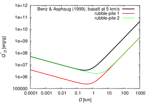
Figure 4: The scaling law for basaltic material at 5 km/s (black line) according to Benz and Asphaug (1999). The red a green lines represent two scaling laws assumed for rubble-pile bodies (1. with less strength than monoliths at all sizes; 2. with less strength than monoliths at large sizes). Their derivations are described in Section 7.

Table 2: Parameters of the scaling law according to Benz and Asphaug (1999) (see Eq. (2)). Parameters $q_{\rm fact}$, $Q_{0}$ and $B$ are the normalization parameters, $a$ and $b$ characterize the slope of the corresponding power law. The procedure how we obtained the parameters for rubble-pile bodies is described in Section 7.

	$\rho$	$Q_{0}$	$a$	$B$	$b$	$q_{\rm fact}$
	(g/cm${}^{3})$	(erg/g)		(erg/g)
basalt	3.00	9$\times 10^{7}$	$-0{.}36$	0.5	1.36	01.0
rubble-pile 1	1.84	9$\times 10^{7}$	$-0{.}36$	0.5	1.36	13.2
rubble-pile 2	1.84	118.8$\times 10^{7}$	$-0{.}36$	0.5	1.36	13.2

5.2 A definition of the $\chi^{2}$ metric

To measure a match between our simulations and the observations we calculate $\chi^{2}$ prescribed by the relation

$$\chi^{2}=\sum^{n}_{i=1}\frac{\left({\rm syn}_{i}-{\rm obs}_{i}\right)^{2}}{\sigma_{i}^{2}}\ ,$$ (3)

where syn_i denotes the synthetic data (i.e. results from Boulder simulations) and obs_i denotes the observed data, $\sigma_{i}$ is the uncertainty of the corresponding obs_i. The quantities syn_i and obs_i are namely the cumulative SFDs $N({>}D)$ or the numbers of families $N_{\rm families}$. More exactly, we calculate $\chi^{2}_{\rm sfd}$ for the 96 points in the cumulative SFDs of the six populations (we verified that this particular choice does not influence our results) and we add $\chi^{2}_{\rm fam}$ for the numbers of families in these populations.

To minimize $\chi^{2}$ we use a simplex numerical method (Press et al., 1992). Another approach we could use is a genetic algorithm which is not-so-prone to “fall” into a local minimum as simplex. Nevertheless, we decided to rather explore the parameter space in a more systematic/controlled way and we start the simplex many times with (729) different initial conditions. We thus do not rely on a single local minimum.

The $\chi^{2}$ prescribed by Eq. (3) is clearly not a “classical” $\chi^{2}$, but a “pseudo”-$\chi^{2}$, because we do not have a well-determined $\sigma_{i}$. Using $\chi^{2}$ we can only decide, if our model corresponds to the observations within the prescribed uncertainties $\sigma_{i}$. Specifically, we used $\sigma_{i}=10\,\%\,$obs_i for the SFDs (similarly as Bottke et al., 2005) and $\sigma_{\rm i}=\sqrt{\rm obs}_{i}$ for the families.

We are aware that the observed $N_{\rm fam}$ values do not follow a Poissonian distribution, and that was actually a motivation for us to use a higher value of weighting for families $w_{\rm fam}=10$ (we multiply $\chi^{2}_{\rm fam}$ by $w_{\rm fam}$), i.e. we effectively decreased the uncertainty of $N_{\rm fam}$ in the $\chi^{2}$ sum. The weighting also emphasizes families, because six values of $\chi^{2}_{\rm fam}$ would have only small influence on the total $\chi^{2}$. Unfortunately, there are still not enough and easily comparable family identifications. Even though there are a number of papers (Parker et al., 2008; Nesvorný, 2012; Masiero et al., 2013; Carruba et al., 2013; Milani et al., 2013), they usually do not discuss parent-body sizes of families.

If a collision between asteroids is not energetic enough (i.e. a cratering event), then only a little of the mass of the target (parent body) is dispersed to the space. In this case, the largest remaining body is called the largest remnant. The second largest body, which has a much lower mass, is called the largest fragment. If a collision is catastrophic, the first two fragments have comparable masses and in such a case, the largest body is called the largest fragment.

In our simulations, we focused on asteroid families with the diameter of the parent body $D_{\rm PB}\geq 100\,{\rm km}$ and the ratio of the largest remnant/fragment to the parent body $M_{\rm LF}/M_{\rm PB}<0.5$ only (i.e. catastrophic disruptions), though the Boulder code treats also cratering events, of course. For that sample we can be quite sure that the observed sample is complete and not biased. This approach is also consistent with the work of Bottke et al. (2005). The numbers of observed families $N_{\rm fam}$ in individual parts are taken from Brož et al. (2013), except for the inner belt, where two additional families were found by Walsh et al. (2013) (i.e. three families in total, see Table 3). Our synthetic families then simply correspond to individual collisions between targets and projectiles — which are energetic enough to catastrophically disrupt the target of given minimum size ($D\geq 100\,{\rm km}$) — as computed by the Boulder code.

In order to avoid complicated computations of the observational bias we simply limit a range of the diameters $D_{\rm max}$ to $D_{\rm min}$ where $\chi^{2}$ is computed (see Table 4) and we admit a possibility that $\chi^{2}$ is slightly increased for $D$ approaching $D_{\rm min}$. We estimated $D_{\rm max}$ and $D_{\rm min}$ for each population separately from the observed SFDs shown in Figure 2.

Table 3: The list of asteroid families in individual parts of the main belt according to Brož et al. (2013) and Walsh et al. (2013). Only families with the diameter of the parent body $D_{\rm PB}>100\,$km and the ratio of the largest remnant/fragment to the parent body $M_{\rm LF}/M_{\rm PB}<0.5$ are listed.

belt	$N_{\rm fam}$	families
inner	3	Erigone	Eulalia	Polana
middle	8	Maria	Padua	Misa
		Dora	Merxia	Teutonia
		Gefion	Hoffmeister
pristine	2	Koronis	Fringilla
outer	6	Themis	Meliboea	Eos
		Ursula	Veritas	Lixiaohua
Cybele	0
high inc.	1	Alauda

Table 4: The ranges of input parameters describing the size-frequency distributions (SFDs) of the six parts of the main belt: $q_{\rm a}$ denotes the slope of the SFD for asteroids with diameters $D>d_{1}$, $q_{\rm b}$ the slope between $d_{1}$ and $d_{2}$, $q_{\rm c}$ the slope for $D<d_{2}$ and $n_{\rm norm}$ is the normalization of the SFD at $d_{1}$. $N_{\rm fam}$ denotes the number of observed families and $D_{\rm max}$ and $D_{\rm min}$ the range of diameters in the SFD, where the $\chi^{2}$ is calculated.

population	$d_{1}$	$d_{2}$	$q_{\rm a}$	$q_{\rm b}$	$q_{\rm c}$	$n_{\rm norm}$	$N_{\rm fam}$	$D_{\rm max}$	$D_{\rm min}$
	(km)	(km)						(km)	(km)
inner	75 to 105	14 to 26	$-3{.}6$ to $-4{.}2$	$-1{.}5$ to $-2{.}7$	$-3{.}0$ to $-4{.}2$	14 to 026	3	250	3
middle	90 to 120	12 to 24	$-4{.}0$ to $-4{.}6$	$-1{.}7$ to $-2{.}9$	$-3{.}0$ to $-4{.}2$	60 to 090	8	250	3
pristine	85 to 115	07 to 19	$-3{.}3$ to $-3{.}9$	$-1{.}8$ to $-3{.}0$	$-3{.}0$ to $-4{.}2$	15 to 027	2	250	5
outer	65 to 095	14 to 26	$-3{.}4$ to $-4{.}0$	$-1{.}9$ to $-3{.}1$	$-2{.}9$ to $-4{.}1$	75 to 105	6	250	5
Cybele	65 to 095	09 to 21	$-2{.}2$ to $-2{.}8$	$-1{.}4$ to $-2{.}6$	$-2{.}2$ to $-3{.}4$	11 to 023	0	250	6
high-inclination	85 to 115	14 to 26	$-3{.}6$ to $-4{.}2$	$-1{.}6$ to $-2{.}8$	$-2{.}9$ to $-4{.}1$	24 to 036	1	250	5

5.3 The Boulder code

A collisional evolution of the size-frequency distributions is modeled with the statistical code called Boulder (Morbidelli et al., 2009), originally developed for studies of the formation of planetary embryos. Our simulations were always running from 0 to 4 Gyr. The Boulder code operates with particles separated to populations, which can differ in values of the intrinsic impact probability $p_{\rm i}$, mutual velocity $v_{\rm imp}$, in material characteristics, etc. The populations are then characterized by their distribution of mass. The total mass range is divided to logarithmic bins, whose width and center evolve dynamically. The processes which are realized in every time step are:

1. the total numbers of collisions among all populations and all mass bins are calculated according to the mutual $p_{\rm i}$’s;

2. the mass of the largest remnant $M_{\rm LR}$ and the largest fragment $M_{\rm LF}$ and the slope $q$ of the SFD of fragments are determined for each collision;

3. the largest remnant and all fragments are distributed to the mass bins of the respective population;

4. it is also possible to prescribe a statistical decay of the populations by dynamical processes;

5. finally, the mass bins are redefined in order to have an optimal resolution and an appropriate next time step $\Delta t$ is chosen.

The relations for $M_{\rm LR}$, $M_{\rm LF}$ and $q$, derived from the works of Benz and Asphaug (1999) and Durda et al. (2007), are

$$M_{\rm LR}=\left[-\frac{1}{2}\left(\frac{Q}{Q^{\star}_{D}}-1\right)+\frac{1}{2}\right]M_{\rm tot}\,\,\,\,\,{\rm for}\,\,Q<Q^{\star}_{D}\,,$$ (4)

$$M_{\rm LR}=\left[-0.35\left(\frac{Q}{Q^{\star}_{D}}-1\right)+\frac{1}{2}\right]M_{\rm tot}\,\,\,\,\,{\rm for}\,\,Q>Q^{\star}_{D}\,,\,\,$$ (5)

$$M_{\rm LF}=8\times 10^{-3}\left[\frac{Q}{Q^{\star}_{D}}\,\exp\left(-\left(\frac{Q}{4Q^{\star}_{D}}\right)^{2}\right)\right]M_{\rm tot}\,,$$ (6)

$$q=-10+7\left(\frac{Q}{Q^{\star}_{D}}\right)^{0.4}\exp\left(-\frac{Q}{7Q^{\star}_{D}}\right)\,,$$ (7)

where $M_{\rm tot}$ denotes the sum of the masses of target and of projectile, $Q^{\star}_{D}$ the strength of the asteroid and $Q$ the specific kinetic energy of the projectile

$$Q=\frac{\frac{1}{2}M_{\rm projectile}v^{2}_{\rm imp}}{M_{\rm tot}}\,.$$ (8)

The disruptions of large bodies have only a small probability during one time step $\Delta t$. In such situations the Boulder uses a pseudo-random-number generator. The processes thus become stochastic and for the same set of initial conditions we may obtain different results, depending on the value of the random seed (Press et al., 1992).

The Boulder code also includes additional “invisible” bins of the SFD (containing the smallest bodies) which should somewhat prevent artificial “waves” on the SFDs, which could be otherwise created by choosing a fixed minimum size.

6 Simulations for monolithic objects

We can expect a different evolution of individual populations as a consequence of their different SFDs, collision probabilities and impact velocities. Therefore, in this Section we are going to run simulations with a new collisional model with six populations.

6.1 An analysis of an extended parameter space

First, we explored the parameter space on larger scales and started the simplex with many different initial conditions (see Figure 5). The calculation had 36 free parameters, as explained above. To reduce the total computational time, we change the same parameter in each part of the main belt with every initialisation of the simplex. For example, we increase all parameters $q_{\rm a1}$, $q_{\rm a2}$, $q_{\rm a3}$, $q_{\rm a4}$, $q_{\rm a5}$, $q_{\rm a\,6}$ together and then we search for a neighbouring local minimum with the simplex which has all 36 parameters free — we call this one cycle. In total, we run $3^{6}=729$ cycles (i.e. initialisations of the simplex), for each parameter we examined 3 values (within the ranges from Table 4). The maximum permitted number of iterations of the simplex was 300 in one cycle (and we verified that this is sufficient to find a $\chi^{2}$ value which is already close to a local minimum). In total, we run 218,700 simulations of the collisional evolution of the main belt.

The argument which would (partly) justify simultaneous changes of all parameters in the 6 parts of the main belt is that we use the same scaling law for each of them, therefore we can expect a similar behaviour in individual belts and it then seems logical to choose initial conditions (SFDs) simultaneously.

The input parameters are summarised in Table 4. The mid-in-the-range values were derived “manually” after several preliminary simulations of collisional evolution (without simplex or $\chi^{2}$ calculations). The changes of parameters between cycles and the steps of simplex within one cycle are listed in Table 5.

Table 5: The changes of input parameters between cycles, and steps of the simplex within one cycle. $d_{1}$, $d_{2}$, $q_{\rm a}$, $q_{\rm b}$, $q_{\rm c}$ and $n_{\rm norm}$ denote the same parameters as in Table 4. For the middle and outer belt, which are more populous, we used $\Delta n_{\rm norm}=15$ and $\delta n_{\rm norm}=5$.

	$d_{1}$	$d_{2}$	$q_{\rm a}$	$q_{\rm b}$	$q_{\rm c}$	$n_{\rm norm}$
	(km)	(km)
cycles	$\pm 15$	$\pm 6$	$\pm 0{.}3$	$\pm 0{.}6$	$\pm 0{.}6$	$\pm$6; 15
steps	5	2	$0{.}1$	$0{.}2$	$0{.}2$	2; 5

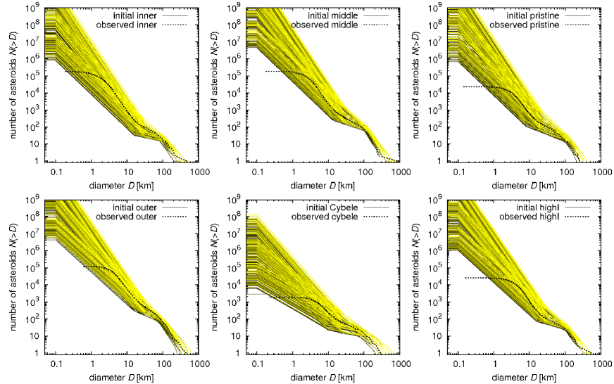
Figure 5: A set of 729 synthetic size-frequency distributions (for six parts of the main belt), which served as starting points for the simplex algorithm and subsequent simulations of collisional evolution. Thin lines (with various colours) denote the synthetic SFDs, while the thick lines corresponds to the observed SFDs. Note that we tested quite a large range of possible initial conditions. The number of simplex steps was limited to 300 because the convergence to a local minimum is difficult due to the stochasticity of the collisional evolution. The total number of collisional simulations we ran was thus $729\times 300=218{,}700$.

The minimum value of $\chi^{2}$, which we obtained, is $\chi^{2}=562$, but we found many other values, that are statistically equivalent (see Figure 6 as an example). Therefore, we did not find a statistically significant global minimum. The parameters $q_{\rm b1-b6}$ seem to be well-determined within the parameter space, parameters $q_{\rm a1-a6}$, $d_{\rm 1\,1-6}$, $d_{\rm 2\,1-6}$ and $n_{\rm norm\,1-6}$ are slightly less constrained. For the remaining parameters $q_{\rm c1-c6}$ we essentially cannot determine the best values. This is caused by the fact that the ‘tail’ of the SFD is created easily during disruptions of larger asteroids, so that the initial conditions essentially do not matter. The influence of the initial conditions at the smallest sizes ($D<d_{2}$) on the final SFDs was carefully checked. As one can see e.g. from the dependence $\chi^{2}(q_{c1})$, i.e. the resulting $\chi^{2}$ values as a function of the initial slope of the tail, the outcome is essentially not dependent on the tail slope, but rather on other free parameters of our model.

Figure 6: The values of $\chi^{2}$ for all simulations of collisional evolution as a function of the parameter $q_{\rm b2}$ (i.e. the slope of the SFD of the middle belt for asteroids with diameters $D<d_{1}$ and $D>d_{2}$). Black points display all initial conditions of the collisional models (within the ranges of the figure), red points display the initial conditions for which simplex converged to a local minimum (i.e. 729 points in total, but less within the ranges of the figure). The dotted line is a value twice larger than the best $\chi^{2}$. Values below this line we consider statistically equivalent. Left: Simultaneous (correlated) changes of parameters in individual parts of the main belt. Right: Randomized (uncorrelated) set of initial parameters (as described in the text).

The differences between simulated and observed SFDs and numbers of families for individual populations corresponding to $\chi^{2}=562$ are shown in Figures 7 and 8. We can see that the largest differences are for the inner and outer belt. Note that it is not easy to improve these results, e.g. by increasing the normalization $n_{\rm norm4}$ of the outer belt, because this would affect all of the remaining populations too.

From Figure 7, we can also assess the influence of the choice of $D_{\rm min}$ and $D_{\rm max}$ values on the resulting $\chi^{2}$ — for example, an increase of $D_{\rm min}$ would mean that the $\chi^{2}$ will be lower (because we would drop several points of comparison this way). However, as this happens in all main belt parts (simultaneously), it cannot change our results significantly. We ran one complete set of simulations with $D_{\rm min}=15\,$km (i.e. with $q_{\rm c}$ unconstrained) to confirm it and we found out that the resulting SFDs, at both larger and smaller sizes than $D_{\rm min}$, are not significantly different from the previous ones.

The parameters of the initial SFDs for the minimal $\chi^{2}$ are summarised in Table 6. Comparing with Table 4, the best initial slopes $q_{\rm a1-6}$ and $q_{\rm c1-6}$ are both significantly steeper than the mid-in-the-range values (from Table 4) and they exceed the value $-3.5$ derived by Dohnanyi. We can also see that the SFD of the Cybele zone is significantly flatter than the SFDs of the other populations and is more affected by observational biases (incompleteness) which actually corresponds to our choice of (relatively large) $D_{\rm min}=6\,{\rm km}$.

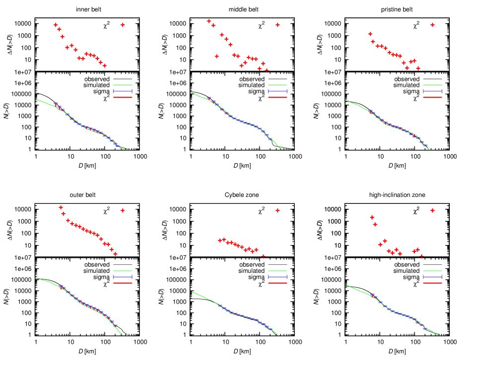
Figure 7: The observed (black line) and simulated (green line) SFDs and the differences between them for the simulation with $\chi^{2}=562$. Sigma errorbars denote the (prescribed) uncertainties of the observed SFDs. This result is for the simulation with monoliths. The largest differences can be seen for the inner and outer belt.

Figure 8: The differences between simulated and observed numbers of families $N_{\rm fam}$ in individual populations, corresponding to the total $\chi^{2}=562$. Sigma errorbars denote the uncertainties of the observed numbers of families. This results is for simulations with monoliths. The simulated and observed numbers of families seem to be consistent within the uncertainties.

Table 6: The parameters describing the initial SFDs (for time $t=-4\,$Gyr) of the six parts of the main belt for which we obtained the best fit ($\chi^{2}=562$) of the observed SFDs and the number of families. $d_{1}$, $d_{2}$, $q_{\rm a}$, $q_{\rm b}$, $q_{\rm c}$ and $n_{\rm norm}$ denote the same parameters as in Table 4 and are rounded to two decimal places.

population	$d_{1}$	$d_{2}$	$q_{\rm a}$	$q_{\rm b}$	$q_{\rm c}$	$n_{\rm norm}$
	(km)	(km)
inner	090.07	20.03	$-4{.}20$	$-2{.}10$	$-4{.}20$	20.03
middle	105.07	18.03	$-4{.}60$	$-2{.}30$	$-4{.}20$	75.07
pristine	100.07	13.03	$-3{.}90$	$-2{.}30$	$-4{.}20$	21.03
outer	080.07	20.03	$-4{.}00$	$-2{.}50$	$-4{.}10$	90.07
Cybele	080.07	15.03	$-2{.}80$	$-2{.}00$	$-3{.}40$	17.03
high-inclination	100.07	20.03	$-4{.}20$	$-2{.}20$	$-4{.}10$	30.03

Another approach to the initial conditions we tested is the following: we generated a completely random set of 729 initial conditions — generated within the ranges simulated previously — and without simultaneous (i.e. with uncorrelated) changes in the 6 parts of the main belt. We then started the simplex algorithms again, i.e. we computed 729 initial conditions for the simplex $\times\,300$ iterations = 218,700 collisional models in total. Results are very similar to the previous ones, with the best $\chi^{2}=544$, which is statistically equivalent to 562, reported above. In Figure 6, we compare the dependence of the $\chi^{2}$ on the parameter $q_{\rm b2}$ for simultaneous (correlated) changes of parameters and for the randomized (uncorrelated) sets of initial parameters. Both results are equivalent in terms of residuals and we can conclude that there is no significantly better local minimum on the interval of parameters we studied.

To test the influence of the choice of $w_{\rm fam}$, we ran simulation with $w_{\rm fam}=0$. The resulting SFDs for monoliths were similar (i.e. exhibiting the same problems) and $\chi^{2}_{\rm sfd}=612$ (among ${\approx}\,$100,000 simulations) remained high. We thus think that the choice of $w_{\rm fam}$ is not critical. While this seems like the families do not determine the result at all, we treat this as an indication that the numbers of families and SFDs are consistent.

6.2 A detailed analysis of the parameters space

We also tried to explore the parameter space in detail — with smaller changes of input parameters between cycles and also smaller steps of the simplex. The best $\chi^{2}$ which we found is however statistically equivalent to the previous value and we did not obtain a significant improvement of the SFDs. Parameters are not well-constrained in this limited parameter space, because the simulations were performed in a surroundings of a local minimum and the simplex was mostly contracting. An even more-detailed exploration of the parameter space thus would not lead to any improvement and we decided to proceed with a model for rubble-pile asteroids.

7 Simulations for rubble-pile objects

The material characteristics of asteroids can significantly influence their mutual collisions. We can modify the Boulder code for rubble-pile bodies on the basis of Benavidez et al. (2012) work, who ran a set of SPH simulation for rubble-pile $D_{\rm PB}=100\,{\rm km}$ parent bodies. We used data from their Fig. 8, namely diameters of fragments inferred for simulations with various projectile diameters and impact velocities.

7.1 Modifications of the Boulder code for rubble-pile bodies

We need to modify the parameters of the scaling law first. We were partly inspired by the shape of scaling laws presented in Levison et al. (2009) for icy bodies (Fig. 3 therein). The modified versions used by these authors are all scaled-down by a factor (i.e. $q_{\rm fact}$ in our notation). Thus, the only two parameters we changed are $q_{\rm fact}$ and density. For the density of asteroids, we used $\rho=1.84\,$g cm^-3 as Benavidez et al. (2012). We determined the specific impact energy $Q^{*}_{D}$ required to disperse half of the total mass of a $D=100\,$km rubble-pile target from the dependence of the mass of the largest remnant $M_{\rm LR}$ as a function of the kinetic energy of projectile $Q$ (see Figure 9). $Q^{*}_{D}$ is then equal to $Q$ corresponding to $M_{\rm LR}/M_{\rm target}=0.5$. So the result is $Q^{*}_{D}=(9\pm 1)\times 10^{7}\,$erg g^-1 and the corresponding parameter $q_{\rm fact}$ in the scaling law is then $13.2\pm 1.5$ (calculated according to Eq. (2) with $\rho=1.84\,$g cm^-3, $r=5\times 10^{6}\,$cm, parameters $Q_{0}$, $a$, $B$ and $b$ remain same as for the monolithic bodies). The scaling law for rubble-pile bodies was already shown graphically in Figure 4 (red line).

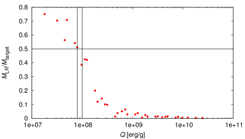
Figure 9: The dependence of the mass of the largest remnant $M_{\rm LR}$ on the kinetic energy $Q$ of the projectile for rubble-pile bodies. We mark the value $M_{\rm LR}/M_{\rm target}=0.5$ with a horizontal line, according to this value we determine $Q_{D}^{*}$. The uncertainties of the determination of $Q^{*}_{D}$ are denoted by vertical lines. The result is $Q^{*}_{D}=(9\pm 1)\times 10^{7}\,$erg g^-1.

We must also derive new dependencies of the slope $q(Q)$ of the fragments’ SFD and for the mass of the largest fragment $M_{\rm LF}(Q)$ on the specific energy $Q$ of the impact. The cumulative SFDs of the fragments cannot be always described with only one single slope. We thus divided the fragments according to their diameters to small ($D<10\,$km) and large ($D>10\,$km) and we determined two slopes. Then we calculated the mean value and we used the differences between the two values as error bars (see Figure 10).

For some of the SPH simulations outcomes it can be difficult to determine the largest fragment, in other words, to distinguish a catastrophic disruption from a cratering event, as explained in Section 5.2. The error bars in Figure 11 correspond to the points, which we would get if we choose the other of the two above-mentioned possibilities.

The parametric relations we determined for rubble-pile bodies are the following

$$q=-6{.}3+3{.}16\left(\frac{Q}{Q^{\star}_{D}}\right)^{0{.}01}\!\!\!\exp\left(-0{.}008\,\frac{Q}{Q_{D}^{\star}}\right),\$$ (9)

$$M_{\rm LF}=\frac{0{.}6}{13\,\left(\frac{Q}{Q^{\star}_{D}}\right)^{-1{.}2}+1{.}5\,\frac{Q}{Q^{\star}_{D}}}{M_{\rm tot}}\,.$$ (10)

When we approximate scattered data with functions, we must carefully check their limits. In the case of low-energetic collisions there is one largest remnant and other fragments are much smaller, therefore for decreasing $Q$ we need $M_{\rm LF}$ to approach zero. The slope $q$ we need to stay negative and not increasing above 0 (that would signify an unphysical power law and zero number of fragments). These conditions are the reasons why our functions do not go through all of the data points (not even within the range of uncertainties). This problem is most pronounced for the dependence of $M_{\rm LF}(Q)$ for small $Q$ (Figure 11). Nevertheless, we think that it is more important that the functions fit reasonably the data for high $Q$’s, because highly-energetic collisions produce a lot of fragments and they influence the SFD much more significantly.

Figure 10: The slope $q$ of the SFD of fragments as a function of the impact energy $Q/Q^{*}_{D}$ for the rubble-pile parent bodies with $D_{\rm PB}=100\,{\rm km}$. The horizontal axis is in a logarithmic scale. The SFD of fragments is characterized by two slopes (for fragments $D<10\,$km and $D>10\,$km) and we calculated the mean value. The displayed uncertainties of $q$ are the differences between real and mean values. The horizontal error bars are given by the uncertainties of $Q^{*}_{D}$. The grey line corresponds to the dependence for monoliths (Morbidelli et al., 2009), which we used in Section 6.

Figure 11: The ratio $M_{\rm LF}/M_{\rm tot}$ (the mass of the largest fragment divided by the sum of the mass of target and the mass of projectile) as a function of the impact energy $Q/Q^{*}_{D}$ for the rubble-pile parent bodies with the diameter $D_{\rm PB}=100\,{\rm km}$. The horizontal axis is in a logarithmic scale. The uncertainties of $M_{\rm LF}/M_{\rm tot}$ are caused by a problematic determination of the largest fragment and the largest remnant. The horizontal error bars are given by the uncertainties of $Q^{*}_{D}$. The grey line corresponds to the dependence for monoliths (Morbidelli et al., 2009) which we used in Section 6.

7.2 A comparison of results for monoliths and rubble-piles with less strength at all sizes

We explored the parameter space in a similar way as for monoliths: with 729 different initial SFDs (i.e. 729 cycles), the maximum permitted number of iterations 300 and 218,700 simulations in total. The changes of parameters between cycles and the steps of the simplex within one cycle are the same as for simulations with monolithic bodies (see Table 5).

The minimum $\chi^{2}$ which we obtained was 1,321. The differences between the simulated and observed SFDs and the numbers of families for individual populations corresponding to $\chi^{2}=1321$ are shown in Figures 12 and 13. These values are significantly higher than what we obtained for monoliths ($\chi^{2}=562$ at best). Given that the set of initial conditions was quite extensive (refer to Figure 5), we think that this difference is fundamental and constitutes a major result of our investigation.

It seems that, at least within our collisional model, we can preliminarily conclude that the main belt does not contain only rubble-pile bodies, because otherwise the corresponding fit would not be that worse than for monoliths (see Figures 7 and 8 for a comparison).

It would be interesting to run a simulation with two different population of the main belt — monolithic and rubble-pile bodies. Also because Benavidez et al. (2012) concluded that some asteroid families were more likely created by a disruption of a rubble-pile parent body: namely the Meliboea, Erigone, Misa, Agnia, Gefion and Rafita. Such simulation remains to be done.

Figure 12: The observed (black line) and simulated (green line) SFDs and the differences between them for the simulation with rubble-piles with total $\chi^{2}=1{,}321$. Sigma errorbars denote the adopted uncertainties of the observed SFDs.

Figure 13: The simulated and the observed numbers of families $N_{\rm fam}$ in individual populations for the simulation with rubble-piles, corresponding to the total $\chi^{2}=1{,}321$. Sigma errorbars denote the uncertainties of the observed numbers of families.

7.3 Simulations for rubble-piles with less strength at large sizes

Large rubble-piles objects can be also assumed to be composed of monolithic blocks with sizes of the order of 100 m. Then, at and below this size, the scaling law $Q^{\star}_{D}$ should be a duplicate of the Benz and Asphaug (1999) — see Figure 4 (green line). We computed a new set of 729 $\times$ 300 = 218,700 collisional simulations with the scaling law modified in this way. The resulting smallest $\chi^{2}$ is 1,393, which should be compared to the previous result $\chi^{2}=1{,}321$ — i.e. no statistically significant improvement.

We thus can conclude that this kind of $Q^{\star}_{D}$ modification does not lead to an improvement of the model. We think that the collisional evolution and overall shape of the SFDs are more affected by disruptions of large asteroids.

8 Improvements and extensions of the model

We think that the match between our collisional model and the observational data as presented in Sections 6 and 7 is not entirely convincing. In this Section we thus try to improve the model by the following procedures: i) We use a longer ‘tail’ of the SFD (down to $D=0.01\,{\rm km}$), which is a straightforward modification. Nevertheless, the longer tail means a significant increase of the required CPU time (which is proportional to $N_{\rm bins}^{2}$). ii) We account for the Yarkovsky effect whose time scales for small bodies ($D\lesssim 0.1\,{\rm km}$) are already comparable to the collisional time scales (see Section 8.1). iii) We do not converge all 36 free parameters at once but we free only 6 of them ($d_{1}$, $d_{2}$, $q_{\rm a}$, $q_{\rm b}$, $q_{\rm c}$ and $n_{\rm norm}$ for one population only) and proceed sequentially with six parts of the main belt (see Section 8.2). iv) Finally, we try to use a scaling law different from Benz and Asphaug (1999) (see Section 8.3).

8.1 Dynamical decay caused by the Yarkovsky effect

In order to improve the Boulder code and use a more complete dynamical model, we try to account for the Yarkovsky effect as follows. We assume that the Yarkovsky effect causes a dynamical decay of the population which can be described by the following relation

$$N(t+\Delta t)=N(t)\exp\left({\Delta t\over\tau_{\rm YE}}\right)\,,$$ (11)

where $N(t)$ denotes the number of bodies at time $t$, $\Delta t$ the time step of the integrator and $\tau_{\rm YE}$ is the characteristic timescale.

We can compute the semimajor-axis drift rate ${\rm d}a/{\rm d}t$, for both the diurnal and seasonal variants of the Yarkovsky effect, using the theory of Vokrouhlický (1998), Vokrouhlický and Farinella (1999) and the (size-dependent) time scale is then

$$\tau_{\rm YE}(D)={\Delta a\over{{\rm d}a/{\rm d}t}(D)}\,,$$ (12)

where $\Delta a$ is the range of semimajor axis given by the positions of major mean-motion resonances which are capable to remove objects from the respective populations. It differs for different zones of the main belt, of course (see Table 7).

In the thermal model, we assume the following parameters: the thermal conductivity $K=0.01\,{\rm W}\,{\rm m}^{-1}\,{\rm K}^{-1}$ for $D>D_{\rm YE}$, i.e. a transition diameter, and $1.0\,{\rm W}\,{\rm m}^{-1}\,{\rm K}^{-1}$ for $D\leq D_{\rm YE}$. The break in $K(D)$ reflects the rotational properties of small bodies, as seen in Figure 14 (and Warner et al. 2009): they rotate too fast, above the critical limit of about 11 revolutions/day, to retain low-conductivity regolith on their surfaces. This is also in accord with infrared observations of Delbo’ et al. (2007), even though the authors propose a linear relationship between the thermal intertia $\Gamma=\sqrt{K\rho C}$ and size $D$ (their Fig. 6), a step-like function may be also compatible with the data. The thermal capacity was $C=680\,{\rm J}\,{\rm kg}^{-1}\,{\rm K}^{-1}$, the infrared emissivity $\epsilon=0.95$ and the Bond albedo $A_{\rm B}=0.02$. The latter value of $A_{\rm B}$ corresponds to the geometric albedo $p_{V}=0.05$, which is typical for C-complex asteroids (e.g. Masiero et al. 2013), with $A_{\rm B}=p_{V}q$, where $q$ denotes the phase integral (with a typical value of 0.39; Bowell et al. 1989). If we assume higher $p_{V}=0.15$ (typical of S-complex) and $A_{\rm B}=0.06$, the Yarkovsky dynamical time scale would remain almost the same, because it is driven by the factor $(1-A_{\rm B})$. Remaining thermal parameters, namely the densities, are summarized in Table 7.

We tested five different models (assumptions):

1. low thermal conductivity $K=0.01\,{\rm W}\,{\rm m}^{-1}\,{\rm K}^{-1}$ only, i.e. $D_{\rm YE}=0\,{\rm km}$, fixed rotation period $P=5\,{\rm h}$;

2. both low/high $K$ with $D_{\rm YE}=200\,{\rm m}$, again $P=5\,{\rm h}$;

3. the same $K(D)$ dependence, but size-dependent spin rate $\omega(D)={2\pi\over P_{0}}{D_{0}\over D}$, $P_{0}=5\,{\rm hour}$, $D_{0}=5\,{\rm km}$;

4. $\omega(D)={2\pi\over P_{0}}\left({D\over D_{0}}\right)^{-1.5}$, $P_{0}=2\,{\rm h}$, $D_{0}=0.2\,{\rm km}$ (see Figure 14);

5. we used Bottke et al. (2005) time scales.

It is important to explain that these spin rate dependencies are not meant to describe bigger asteroids but rather smaller ones ($D\lesssim 1\,{\rm km}$) that comprise the majority of impactors but mostly fall below the detection threshold.

We then computed the Yarkovsky time scales $\tau_{\rm YE}(D)$ (Figure 15) and constructed a ‘testing’ collisional model in order to check the influence of the dynamical decay on the evolution of the main belt SFD. Note that for small sizes $D\lesssim 1\,{\rm km}$, $\tau_{\rm YE}(D)$ can be even smaller than corresponding collisional time scales $\tau_{\rm col}(D)$.

Regarding the asteroid families, we use the most straightforward approach: we simply count only families large enough (original $D_{\rm PB}>100\,{\rm km}$, $m_{\rm LR}/m_{\rm PB}<0.5$) which cannot be completely destroyed by a collisional cascade (Bottke et al., 2005) or by the Yarkovsky drift (Bottke et al., 2001). We verified this statement (implicitly) also in our recent work (Brož et al., 2013) in which the evolution of SFDs for individual synthetic families was studied. At the same time, we use original parent-body sizes $D_{\rm PB}$ of the observed families — inferred by using methods of Durda et al. (2007) or Tanga et al. (1999); as summarised in Brož et al. (2013) — so that we can directly compare them to synthetic families, as output from the Boulder code.

The results of models 1 and 2 above are clearly not consistent with the observed SFD (see Figure 16). The results of 3, 4 and 5 seem to be equivalent and consistent with observations, however, we cannot distinguish between them. We can thus exclude ‘extreme’ Yarkovsky drift rates and conclude that only lower or ‘reasonable’ drift rates provide a reasonable fit to the observed SFD of the main belt.

Table 7: The parameters of the Yarkovsky-driven decay which are dependent on the zone of the main asteroid belt: $\Delta a$ is half of the zone size (or a typical distance from neighbouring strong mean-motion resonances), $\rho$ denotes the (bulk and surface) density assumed for respective bodies.

	$\Delta a$	$\rho$
zone	AU	${\rm kg}\,{\rm m}^{-3}$
inner	0.2	2,500
middle	0.1615	2,500
pristine	0.0665	1,300
outer	0.162	1,300
Cybele	0.105	1,300
high-$I$	0.135	1,300

Figure 14: The spin rate $\omega$ vs size $D$ dependence for asteroids (observational data from Warner et al., 2009), the Lost City fireball (Ceplecha, 1996) and fragments in laboratory experiments (Giblin et al., 1998). Two approximations are given: $\omega(D)\propto 1/D$, and $\omega(D)\propto D^{-1.5}$, which better fits the observational data in the size range $D\in(0.01,1)\,{\rm km}$ where the Yarkovsky drift is the most important with respect to the collisional model. Nevertheless, we cannot yet exclude a possibility that the observed $\omega(D)$ distribution is still strongly biased for small $D\lesssim 1\,{\rm km}$.

Figure 15: The time scale $\tau_{\rm YE}$ of the Yarkovsky-driven decay (as defined by Eq. 12) vs size $D$ for three different models (denoted 1, 3 and 5), or in other words, assumptions of the thermal conductivity $K(D)$ and the spin rate $\omega(D)$, which were described in the text. The obliquities $\gamma$ of the spin axes were assumed moderate, $|\gamma|=45^{\circ}$. Model 2 is quite similar to 1 and model 4 is similar to 3, so we decided not to plot them in order to prevent many overlapping lines. For each model, we plot six lines corresponding to the six zones of the main belt: inner, middle, ‘pristine’, outer, Cybele and high inclination. Bottke et al. (2005) time scales were used for the whole main belt (regarded as a single population).

Figure 16: Resulting synthetic size-frequency distributions of the main belt (regarded as a single population) after 4 Gyr of collisional evolution, as computed by the Boulder code. We show results for three different models of the Yarkovsky-driven decay (denoted 1, 3 and 5 in the text). Model 1 (dotted line) is clearly inconsistent with the observed SFD (thick gray line). The shaded region corresponds to the sizes well below the observational completeness.

8.2 Subsequent fits for individuals parts of the main belt

In order to improve our ‘best’ fit from Section 6 (and 7), we ran simplex sequentially six times, with only 6 parameters free in each case, namely $d_{1}$, $d_{2}$, $q_{\rm a}$, $q_{\rm b}$, $q_{\rm c}$, $n_{\rm norm}$ for a given part of the main belt. We included a longer tail ($D_{\rm min}=0.01\,{\rm km}$) and the Yarkovsky model discussed above. The number of simplex iterations was always limited to 100.

We shall not be surprised if we obtain a $\chi^{2}$ value which is (slightly) larger than before because we changed the collisional model and this way we moved away from the previously-found local minimum. At the same time, we do not perform that many iterations as before (600 vs. 218,700), so we cannot ‘pick-up’ the deepest local minima.

For monoliths, we tried to improve the ‘best’ fit with $\chi^{2}=562$. However, the initial value at the very start of the simplex was ${\chi^{2}}^{\prime}\simeq 803$ (due to the changes in the collisional model) and the final value after the six subsequent fits ${\chi^{2}}^{\prime\prime}=520$. This is only slightly smaller than the previous $\chi^{2}$ and statistically equivalent (${\chi^{2}}^{\prime\prime}\simeq\chi^{2}$). For rubble-piles, a similar procedure for the $\chi^{2}=1{,}321$ fit lead to the initial ${\chi^{2}}^{\prime}\simeq 1{,}773$ and the final ${\chi^{2}}^{\prime\prime}=1{,}470$. Again, a statistically-equivalent result.

We interpret this as follows: our simplex algorithm naturally selects deep local minima. It seems that the lowest $\chi^{2}$ (for a given set of initial conditions) can be achieved by a ‘lucky’ sequence of disruptions of relatively large bodies ($D_{\rm PB}\gtrsim 100\,{\rm km}$) which results in synthetic SFDs and the numbers of families best matching the observed properties. Of course, this sequence depends on the ‘seed’ value of the random-number generator.

To conclude, our improvements of the collisional model do not seem significant and the $\chi^{2}$ values are of the same order. This can be considered as an indication that we should probably use an even more complicated model. (Nevertheless, there is still a significant difference between monoliths and rubble-piles and the assumption of monolithic structure matches the observations better.)

8.3 Simulations with various scaling laws

So far we used the scaling law of Benz and Asphaug (1999) for all simulations. In this Section, we are going to test different scaling laws. Similarly as Bottke et al. (2005), we changed the specific impact energy $Q_{D}^{*}$ of asteroids with $D>200\,$m (see Figure 17, left). For each scaling law we ran 100 simulations of the collisional evolution with different random seeds. The initial parameters of SFDs are fixed and correspond to the best-fit initial parameters found in Section 6.

In order to decide which scaling laws are suitable, we can simply compare the resulting synthetic SFDs and the numbers of families to the observed ones. It is clear that if we increase the strength of $D\simeq 100\,{\rm km}$ bodies by a factor of 10 or more, the number of synthetic families (namely catastrophic disruptions with $D_{\rm PB}\geq 100\,{\rm km}$) is much smaller than the observed number (usually 4 vs 20, see in Figure 17, middle). On the other hand, if we decrease the strength by a factor of 10, the synthetic SFDs exhibit a significant deficit of small bodies with $D<10\,{\rm km}$ due to a collisional cascade (especially in the inner belt, see Figure 17, right). Moreover, the number of synthetic families is then significantly larger, of course. The fact that the number of synthetic families is dependent on the scaling law confirm our statement that families are important observational constraints.

These results lead us to the conclusion, that the ‘extreme’ scaling laws (i.e. much different from Benz and Asphaug, 1999) cannot be used for the main asteroid belt. This result is also in accord with Bottke et al. (2005).

Figure 17: Left: A number of scaling laws with modified strength of large bodies (a similar set as in Bottke et al., 2005). The red line represents the nominal scaling law of Benz and Asphaug (1999). Middle: Histograms representing the number $N$ of simulations (out of 100) a given number of families $N_{\rm families}$ was created; we assumed the scaling law with an increased strength of large bodies ($b=1.9$). The observed numbers of families are displayed as filled circles for comparison. Right: The final size-frequency distributions of the inner belt for 100 simulations with different random seeds and for the scaling law with a decreased strength of large bodies ($b=1.0$). Neither of these two mentioned simulations is consistent with the observations (their $\chi^{2}$ would be clearly much larger than the best fit from Section 6).

9 Conclusions

In this work, we created a new collisional model of the evolution of the main asteroid belt. We divided the main belt into six parts and constructed the size-frequency distribution for each part. The observed SFDs differ significantly in terms of slopes and total numbers of asteroids. We then ran two sets of simulations — for monolithic bodies and for rubble-piles.

In the case of monoliths, there seem to be (relatively minor) discrepancies between the simulated and observed SFDs in individual parts of the main belt, nevertheless, the numbers of families (catastrophic disruptions) correspond within uncertainties. On the other hand, the $\chi^{2}$ value for rubble-pile bodies is more than twice as large because there are systematic differences between the SFDs and the number of families is substantially larger (usually 30 or more) than the observed one (20 in total). We can thus conclude that within our collisional model, monolithic asteroids provide a better match to the observed data than rubble-piles, even though we cannot exclude a possibility that a certain part of the population is indeed of rubble-pile structure, of course.

We tried to improve our model by: (i) introducing a longer ‘tail’ of the SFD (down to $D=0.01\,{\rm km}$); (ii) incorporating the Yarkovsky effect, i.e. a size-dependent dynamical decay; (iii) running many simulations with different random seeds, in order to find even low-probability scenarios. Neither of these improvements provided a substantially better match in all parts of the main belt at once.

However, we can think of several other possible reasons, why the match between our collisional model and the observed SFDs is not perfect:

1. There are indeed different scaling laws for different parts of the main belt. This statement could be supported by the observed distribution of albedo, which is not uniform in the main belt, and by the diverse compositions of asteroids (DeMeo and Carry, 2014). This topic is a natural continuation of our work (and a detailed analysis is postponed to a forthcoming paper).

2. The scaling of the SPH simulations from $D_{\rm PB}=100\,{\rm km}$ by one or even two orders of magnitude is likely problematic. Our work is thus a motivation to study disruptions of both smaller ($D_{\rm PB}\simeq 1\,{\rm km}$) and larger ($400\,{\rm km}$) targets. Similar sets of SPH simulations as in Durda et al. (2007) and Benavidez et al. (2012) would be very useful for further work.

3. To explain the SFD of the inner belt, namely its ‘tail’, we would need to assume a recent disruption (during the last $\sim 100\,{\rm Myr}$) of a large parent body ($D_{\rm PB}\gtrsim 200\,{\rm km}$). In that case the SFD is temporarily steep — and may be closer to the observed SFD in the particular part of the main belt — but only for a limited period of time which is typically about 200 Myr. After that time, the collisional cascade eliminates enough bodies and consequently the SFD becomes flatter. On the other hand, there must not have occurred a recent large disruption in the middle or the outer belt, otherwise the synthetic SFD is more populous than the observed one. It is not likely, that all such conditions are fulfilled together in our model, in which collisions occur randomly.

4. When we split the main belt into 6 parts, the evolution seems too stochastic (the number of large events in individual part is of the order of 1). It may be even useful to prepare a ‘deterministic model’, in which large disruptions are prescribed, according to the observed families and their ages. Of course, the completeness of the family list and negligible bias are then crucial.

5. Our model does not yet include an YORP-induced fission (Marzari et al., 2011), even though there are indications that these ‘additional’ disruptions might affect the tail of the SFD if they are frequent enough as stated by Jacobson et al. (2014).

6. We can improve the modelling of the Yarkovsky/YORP effect, e.g. by assuming a more realistic distribution of spin rates (not only the $\omega(D)$ dependence, Figure 14) and performing an $N$-body simulation of the orbital evolution to get a more accurate estimate of the (exponential) time scale $\tau_{\rm YE}(D)$. It may be difficult to estimate biases in the $\omega(D)$ plot, because the respective dataset is heterogeneous. Luckily, the Gaia spacecraft is expected to provide a large homogeneous database of asteroid spin properties (Mignard et al., 2007).

7. May be, the intrinsic collisional probabilities $p_{\rm i}$ were substantially different (lower) in the past, e.g. before major asteroid families were created (as suggested by Dell’Oro et al. 2001).

8. Some of the mutual impact velocities $v_{\rm imp}$, especially with high-inclination objects, are substantially larger than the nominal $5\,{\rm km}\,{\rm s}^{-1}$, so the outcomes of these collisions are most-likely different. On the other hand, these collisions are usually of lower probability and the high-inclination region is not that populous, so that this effect has likely a minor contribution only. One should properly account for observational biases acting against discoveries of high-inclination objects, thought (Novaković et al., 2011).

9. Collisions occur not only at the mean impact velocity $v_{\rm imp}$, but there is rather a distribution of velocities. It would be then useful and logical to use a velocity-dependent scaling law (Leinhardt and Stewart, 2012; Stewart and Leinhardt, 2009).

10. There might be several large undiscovered families, or in other words, the lists of $D_{\rm PB}\leq 100\,{\rm km}$ families (Brož et al. 2013, or Masiero et al. 2013) might be strongly biased, because comminution is capable to destroy most of the fragments.

11. Possibly, parent-body sizes $D_{\rm PB}$ of the observed families are systematically underestimated or their mass ratios $M_{\rm LR}/M_{\rm PB}$ of the largest remnant to parent body are offset, even though they were determined by best available methods (Durda et al., 2007; Tanga et al., 1999).

The topics outlined above seem to be good starting points for (a lot of) further work.

References

- Benavidez et al. (2012) Benavidez, P. G., Durda, D. D., Enke, B. L., Bottke, W. F., Nesvorný, D., Richardson, D. C., Asphaug, E., Merline, W. J., May 2012. A comparison between rubble-pile and monolithic targets in impact simulations: Application to asteroid satellites and family size distributions. Icarus 219, 57–76.
- Benz and Asphaug (1999) Benz, W., Asphaug, E., Nov. 1999. Catastrophic Disruptions Revisited. Icarus 142, 5–20.
- Bottke et al. (2005) Bottke, W. F., Durda, D. D., Nesvorný, D., Jedicke, R., Morbidelli, A., Vokrouhlický, D., Levison, H., May 2005. The fossilized size distribution of the main asteroid belt. Icarus 175, 111–140.
- Bottke and Greenberg (1993) Bottke, W. F., Greenberg, R., May 1993. Asteroidal collision probabilities. Geophys. Res. Lett. 20, 879–881.
- Bottke et al. (2002) Bottke, W. F., Morbidelli, A., Jedicke, R., Petit, J.-M., Levison, H. F., Michel, P., Metcalfe, T. S., Apr. 2002. Debiased Orbital and Absolute Magnitude Distribution of the Near-Earth Objects. Icarus 156, 399–433.
- Bottke et al. (2001) Bottke, W. F., Vokrouhlický, D., Broz, M., Nesvorný, D., Morbidelli, A., Nov. 2001. Dynamical Spreading of Asteroid Families by the Yarkovsky Effect. Science 294, 1693–1696.
- Bottke et al. (2006) Bottke, Jr., W. F., Vokrouhlický, D., Rubincam, D. P., Nesvorný, D., May 2006. The Yarkovsky and Yorp Effects: Implications for Asteroid Dynamics. Annual Review of Earth and Planetary Sciences 34, 157–191.
- Bowell et al. (1989) Bowell, E., Hapke, B., Domingue, D., Lumme, K., Peltoniemi, J., Harris, A. W., 1989. Application of photometric models to asteroids. In: Binzel, R. P., Gehrels, T., Matthews, M. S. (Eds.), Asteroids II. pp. 524–556.
- Brož et al. (2013) Brož, M., Morbidelli, A., Bottke, W. F., Rozehnal, J., Vokrouhlický, D., Nesvorný, D., Mar. 2013. Constraining the cometary flux through the asteroid belt during the late heavy bombardment. Astron. Astrophys. 551, A117.
- Carruba et al. (2013) Carruba, V., Domingos, R. C., Nesvorný, D., Roig, F., Huaman, M. E., Souami, D., Aug. 2013. A multidomain approach to asteroid families’ identification. Mon. Not. R. Astron. Soc. 433, 2075–2096.
- Carry (2012) Carry, B., Dec. 2012. Density of asteroids. Plan. and Space Science 73, 98–118.
- Cellino et al. (1991) Cellino, A., Zappala, V., Farinella, P., Dec. 1991. The size distribution of main-belt asteroids from IRAS data. Mon. Not. R. Astron. Soc. 253, 561–574.
- Ceplecha (1996) Ceplecha, Z., Jul. 1996. Luminous efficiency based on photographic observations of the Lost City fireball and implications for the influx of interplanetary bodies onto Earth. Astron. Astrophys. 311, 329–332.
- Dahlgren (1998) Dahlgren, M., Aug. 1998. A study of Hilda asteroids. III. Collision velocities and collision frequencies of Hilda asteroids. Astron. Astrophys. 336, 1056–1064.
- Davis et al. (1979) Davis, D. R., Chapman, C. R., Greenberg, R., Weidenschilling, S. J., Harris, A. W., 1979. Collisional evolution of asteroids - Populations, rotations, and velocities. pp. 528–557.
- Delbo’ et al. (2007) Delbo’, M., dell’Oro, A., Harris, A. W., Mottola, S., Mueller, M., Sep. 2007. Thermal inertia of near-Earth asteroids and implications for the magnitude of the Yarkovsky effect. Icarus 190, 236–249.
- Dell’Oro and Paolicchi (1998) Dell’Oro, A., Paolicchi, P., Dec. 1998. Statistical Properties of Encounters among Asteroids: A New, General Purpose, Formalism. Icarus 136, 328–339.
- Dell’Oro et al. (2001) Dell’Oro, A., Paolicchi, P., Cellino, A., Zappalà, V., Tanga, P., Michel, P., Sep. 2001. The Role of Families in Determining Collision Probability in the Asteroid Main Belt. Icarus 153, 52–60.
- DeMeo and Carry (2014) DeMeo, F. E., Carry, B., Jan. 2014. Solar System evolution from compositional mapping of the asteroid belt. Nature 505, 629–634.
- Dohnanyi (1969) Dohnanyi, J. S., May 1969. Collisional Model of Asteroids and Their Debris. J. Geophys. Res. 74, 2531.
- Durda et al. (2007) Durda, D. D., Bottke, W. F., Nesvorný, D., Enke, B. L., Merline, W. J., Asphaug, E., Richardson, D. C., Feb. 2007. Size-frequency distributions of fragments from SPH/N-body simulations of asteroid impacts: Comparison with observed asteroid families. Icarus 186, 498–516.
- Giblin et al. (1998) Giblin, I., Martelli, G., Farinella, P., Paolicchi, P., di Martino, M., Smith, P. N., Jul. 1998. The Properties of Fragments from Catastrophic Disruption Events. Icarus 134, 77–112.
- Greenberg (1982) Greenberg, R., Jan. 1982. Orbital interactions - A new geometrical formalism. Astron. J. 87, 184–195.
- Hodapp et al. (2004) Hodapp, K. W., Kaiser, N., Aussel, H., Burgett, W., Chambers, K. C., Chun, M., Dombeck, T., Douglas, A., Hafner, D., Heasley, J., Hoblitt, J., Hude, C., Isani, S., Jedicke, R., Jewitt, D., Laux, U., Luppino, G. A., Lupton, R., Maberry, M., Magnier, E., Mannery, E., Monet, D., Morgan, J., Onaka, P., Price, P., Ryan, A., Siegmund, W., Szapudi, I., Tonry, J., Wainscoat, R., Waterson, M., Oct. 2004. Design of the Pan-STARRS telescopes. Astronomische Nachrichten 325, 636–642.
- Jacobson et al. (2014) Jacobson, S. A., Marzari, F., Rossi, A., Scheeres, D. J., Davis, D. R., Mar. 2014. Effect of rotational disruption on the size-frequency distribution of the Main Belt asteroid population. Mon. Not. R. Astron. Soc. 439, L95–L99.
- Knežević and Milani (2003) Knežević, Z., Milani, A., Jun. 2003. Proper element catalogs and asteroid families. Astron. Astrophys. 403, 1165–1173.
- Leinhardt and Stewart (2012) Leinhardt, Z. M., Stewart, S. T., Jan. 2012. Collisions between Gravity-dominated Bodies. I. Outcome Regimes and Scaling Laws. Astrophys. J. 745, 79.
- Levison et al. (2009) Levison, H. F., Bottke, W. F., Gounelle, M., Morbidelli, A., Nesvorný, D., Tsiganis, K., Jul. 2009. Contamination of the asteroid belt by primordial trans-Neptunian objects. Nature 460, 364–366.
- Mainzer et al. (2011) Mainzer, A., Grav, T., Masiero, J., Bauer, J., Wright, E., Cutri, R. M., McMillan, R. S., Cohen, M., Ressler, M., Eisenhardt, P., Aug. 2011. Thermal Model Calibration for Minor Planets Observed with Wide-field Infrared Survey Explorer/NEOWISE. Astrophys. J. 736, 100.
- Marzari et al. (2011) Marzari, F., Rossi, A., Scheeres, D. J., Aug. 2011. Combined effect of YORP and collisions on the rotation rate of small Main Belt asteroids. Icarus 214, 622–631.
- Masiero et al. (2013) Masiero, J. R., Mainzer, A. K., Bauer, J. M., Grav, T., Nugent, C. R., Stevenson, R., Jun. 2013. Asteroid Family Identification Using the Hierarchical Clustering Method and WISE/NEOWISE Physical Properties. Astrophys. J. 770, 7.
- Masiero et al. (2011) Masiero, J. R., Mainzer, A. K., Grav, T., Bauer, J. M., Cutri, R. M., Dailey, J., Eisenhardt, P. R. M., McMillan, R. S., Spahr, T. B., Skrutskie, M. F., Tholen, D., Walker, R. G., Wright, E. L., DeBaun, E., Elsbury, D., Gautier, IV, T., Gomillion, S., Wilkins, A., Nov. 2011. Main Belt Asteroids with WISE/NEOWISE. I. Preliminary Albedos and Diameters. Astrophys. J. 741, 68.
- Michel et al. (2011) Michel, P., Jutzi, M., Richardson, D. C., Benz, W., Jan. 2011. The Asteroid Veritas: An intruder in a family named after it? Icarus 211, 535–545.
- Mignard et al. (2007) Mignard, F., Cellino, A., Muinonen, K., Tanga, P., Delbò, M., Dell’Oro, A., Granvik, M., Hestroffer, D., Mouret, S., Thuillot, W., Virtanen, J., Dec. 2007. The Gaia Mission: Expected Applications to Asteroid Science. Earth Moon and Planets 101, 97–125.
- Milani et al. (2013) Milani, A., Cellino, A., Knezevic, Z., Novakovic, B., Spoto, F., Paolicchi, P., Dec. 2013. Asteroid families classification: exploiting very large data sets. ArXiv e-prints.
- Morbidelli et al. (2009) Morbidelli, A., Bottke, W. F., Nesvorný, D., Levison, H. F., Dec. 2009. Asteroids were born big. Icarus 204, 558–573.
- Nesvorný (2010) Nesvorný, D., Nov. 2010. Nesvorný HCM Asteroid Families V1.0. NASA Planetary Data System 133.
- Nesvorný (2012) Nesvorný, D., Jun. 2012. Nesvorný HCM Asteroid Families V2.0. NASA Planetary Data System 189.
- Nesvorný et al. (2005) Nesvorný, D., Jedicke, R., Whiteley, R. J., Ivezić, Ž., Jan. 2005. Evidence for asteroid space weathering from the Sloan Digital Sky Survey. Icarus 173, 132–152.
- Novaković et al. (2011) Novaković, B., Cellino, A., Knežević, Z., Nov. 2011. Families among high-inclination asteroids. Icarus 216, 69–81.
- Parker et al. (2008) Parker, A., Ivezić, Ž., Jurić, M., Lupton, R., Sekora, M. D., Kowalski, A., Nov. 2008. The size distributions of asteroid families in the SDSS Moving Object Catalog 4. Icarus 198, 138–155.
- Press et al. (1992) Press, W. H., Teukolsky, S. A., Vetterling, W. T., Flannery, B. P., 1992. Numerical recipes in FORTRAN. The art of scientific computing.
- Stewart and Leinhardt (2009) Stewart, S. T., Leinhardt, Z. M., Feb. 2009. Velocity-Dependent Catastrophic Disruption Criteria for Planetesimals. Astrophys. J. Lett. 691, L133–L137.
- Stuart (2001) Stuart, J. S., Nov. 2001. A Near-Earth Asteroid Population Estimate from the LINEAR Survey. Science 294, 1691–1693.
- Tanga et al. (1999) Tanga, P., Cellino, A., Michel, P., Zappalà, V., Paolicchi, P., dell’Oro, A., Sep. 1999. On the Size Distribution of Asteroid Families: The Role of Geometry. Icarus 141, 65–78.
- Tedesco et al. (2005) Tedesco, E. F., Bottke, W. F., Bus, S. J., Volquardsen, E., Cellino, A., Delbo, M., Davis, D. R., Morbidelli, A., Hora, J. L., Adams, J. D., Kassis, M., Aug. 2005. Albedo Distributions of Near-Earth and Intermediate Source Region Asteroids. In: AAS/Division for Planetary Sciences Meeting Abstracts #37. Vol. 37 of Bulletin of the American Astronomical Society. p. 643.
- Tedesco et al. (2002) Tedesco, E. F., Noah, P. V., Noah, M., Price, S. D., Feb. 2002. The Supplemental IRAS Minor Planet Survey. Astron. J. 123, 1056–1085.
- Vokrouhlický (1998) Vokrouhlický, D., Jul. 1998. Diurnal Yarkovsky effect as a source of mobility of meter-sized asteroidal fragments. I. Linear theory. Astron. Astrophys. 335, 1093–1100.
- Vokrouhlický and Farinella (1999) Vokrouhlický, D., Farinella, P., Dec. 1999. The Yarkovsky Seasonal Effect on Asteroidal Fragments: A Nonlinearized Theory for Spherical Bodies. Astron. J. 118, 3049–3060.
- Walsh et al. (2013) Walsh, K. J., Delbó, M., Bottke, W. F., Vokrouhlický, D., Lauretta, D. S., Jul. 2013. Introducing the Eulalia and new Polana asteroid families: Re-assessing primitive asteroid families in the inner Main Belt. Icarus 225, 283–297.
- Warner et al. (2009) Warner, B. D., Harris, A. W., Pravec, P., Jul. 2009. The asteroid lightcurve database. Icarus 202, 134–146.
- Zappalà et al. (1995) Zappalà, V., Bendjoya, P., Cellino, A., Farinella, P., Froeschlé, C., Aug. 1995. Asteroid families: Search of a 12,487-asteroid sample using two different clustering techniques. Icarus 116, 291–314.